Path Planning and Task Assignment for Data Retrieval from Wireless Sensor Nodes Relying on Game-Theoretic Learning

Abstract

The energy-efficient trip allocation of mobile robots employing differential drives for data retrieval from stationary sensor locations is the scope of this article. Given a team of robots and a set of targets (wireless sensor nodes), the planner computes all possible tours that each robot can make if it needs to visit a part of or the entire set of targets. Each segment of the tour relies on a minimum energy path planning algorithm. After the computation of all possible tour-segments, a utility function penalizing the overall energy consumption is formed. Rather than relying on the NP-hard Mobile Element Scheduling (MES) MILP problem, an approach using elements from game theory is employed. The suggested approach converges fast for most practical reasons thus allowing its utilization in near real time applications. Simulations are offered to highlight the efficiency of the developed algorithm.

I Introduction

A typical Wireless Sensor Network (WSN) [1] consists of a number of low power, static sensor nodes scattered in the environment and a base station. The nodes need to transfer the data collected by their sensors back to the base station in an energy efficient manner. Given the low transmission power of the nodes, a WSN consisting solely of static nodes would require a large number of densely placed relay nodes in order to transmit the data to the base station. This approach however significantly increases the cost of the WSN and makes large scale deployment more difficult.

In order to counteract this problem, the usage of mobile robots as data mules has been proposed [2, 3]. The robots download data from one or more sensor nodes and upload it to the base station. Since the sensor nodes have a limited amount of on-board memory, the data mule robots must visit each node in a timely fashion which is called the Mobile Element Scheduling (MES) problem [4]. The problem of planning a route for each data mule robot is an NP-hard optimization problem which is formulated as the Traveling Salesman Subset-tour Problem (TSSP) [5].

Moreover, the limited battery capacity of the mobile robots has to be taken into account when planning the routes of the mobile robots. To that extent an energy model of the mobile robots is required. Work has been done in both the energy modeling [6] of various types of ground robots as well as energy efficient path planning for them [7, 8].

In this article we assume a team of car-like robots which act as data mules in a WSN. Our goal is to create energy efficient paths so that the team of mobile robots collectively visits all sensor nodes. In order to avoid the computationally expensive Mixed-Integer Linear Programming (MILP) problem associated with finding the optimal solution to the TSSP, we formulate the problem as a cooperative game and employ game theoretic learning algorithms. Although these algorithms converge to suboptimal solutions, they are typically magnitudes faster compared to MILP. Thus the main contribution of this article is the utilization of game-theoretic learning techniques in order to reduce the computational burden of routing the data mules, while also providing energy efficient trajectories by incorporating path energy costs into the game utility function.

Section II presents the particular problem under consideration and outlines the way it is approached. Section III presents the agent model as well as the derivation of energy efficient paths and velocity profiles based on that model. Section IV provides some theoretical background on the game-theoretic methods and algorithms used. Section V defines the particular utility function defined for the problem. Section VI provides several comparative simulation studies between various game-theoretic learning algorithms and is followed by concluding remarks.

II Problem statement

We assume $M$ sensor nodes comprising a WSN and dispersed in a convex region $\Omega\subset\mathbb{R}^{2}$ at positions $P_{j}\in\Omega,\ j\in I_{M}$, where $I_{M}=\left\{1,\ \dots,\ M\right\}$. We also assume a team of $N$ mobile robots with initial poses $Q_{i}^{0}=\left[{q_{i}^{0}}^{T}\ \theta_{i}^{0}\right]\in\Omega\times\left[-\pi,\pi\right]$ which act as data mules for the sensor nodes. The goal of the robot team is to collectively visit all sensor nodes and return to its initial position, while also reducing the total energy consumption as much as possible.

In order to formulate the aforementioned problem as a game, we need to define the action space of each robot agent. The action of each agent consists of a sequence of sensor nodes, which essentially defines a route for the agent. However, as the size of the WSN increases, the quick growth of the action space of each agent makes the problem infeasible computationally. In order to combat this problem, we use two techniques outlined in the sequel.

First, by imposing a maximum number $M^{\max}$ of sensor nodes any single agent may visit during a single route, we can effectively limit the size of the action space. This constraint makes sense from a practical point of view as well, since a single agent may not have a large enough energy capacity in order to visit a large number of nodes without the need to recharge. Using the upper limit in the number of nodes to visit, the number of available actions $A_{i}$ for a single agent is:

$$A_{i}=1+\sum_{k=1}^{M^{\max}}\frac{M!}{(M-k)!},$$

where one is added in order to include the case of the agent visiting zero sensor nodes.

In addition, especially in the case of large WSNs, it does not make sense for some agent $i$ to cover a large distance in order to visit a sensor node $j$ which is significantly closer to one or more other agents. More importantly, the robot agent need to communicate in order to choose their routes in a cooperative manner, but due to their finite communication range, only agents in relative proximity will be able to do so. To that extent, we split the robot team into groups consisting of agents whose communication graph is fully connected. After the robot team has been split into sub-teams, each sub-team can be assigned a region of responsibility and be responsible for visiting only the sensor nodes inside this region. One of the possible methods for assigning regions of responsibility is using the Generalized Voronoi diagram [9].

The Generalized Voronoi diagram for a set of $n$ planar sites $H_{i},\ i\in I_{N}$ inside some planar region $\Omega$ is defined as:

$$V_{i}=\left\{q\in\Omega\colon d\left(q,H_{i}\right)\leq d\left(q,H_{j}\right),\ \forall j\neq i\right\},\ i\in I_{N}$$

where $d\left(q,D\right)=\min\left\{\parallel q-p\parallel,\forall p\in D\right\}$. By computing the convex hull of the robot positions of each group, we can represent each group by a convex polygon. We can then compute the Generalized Voronoi diagram using these polygons as seeds and thus assigning a region of responsibility to each group. This procedure is illustrated in Figure 1, where agent groups and their communication links are shown in colored lines, the sensor nodes are marked with black triangles and the boundaries of the Generalized Voronoi diagram are shown in dashed gray.

Figure 1: Splitting of the robot team into subgroups and region assignment using the Generalized Voronoi diagram.

III Energy efficient path computation

III-A Agent Kinematic Model

In order to compute energy efficient paths, an appropriate agent model is required. The agent model used is the same car-like model as the one in [8]. Each agent’s kinematic model is

$$\dot{q}_{i} =\left[\begin{array}[]{c}\cos\theta_{i}\\ \sin\theta_{i}\end{array}\right]\ v_{i}, q_{i}\in\Omega,\ v_{i}\in\left[0,\ v^{\max}\right],$$

$$\dot{v}_{i} =a_{i}, a_{i}\in\mathbb{R},$$

$$\dot{\theta}_{i} =\psi_{i}, \theta_{i}\in\left[-\pi,\ \pi\right],\ \psi_{i}\in\mathbb{R},$$

where $q_{i}$ is the agent’s position, $\theta_{i}$ its orientation, $v_{i}$ its linear velocity and $a_{i},\ \psi_{i}$ its linear acceleration and angular velocity control inputs. There is an upper bound $v^{\max}$ for the velocity of the agent, while its velocity may not be negative, thus it can not move in reverse. It is assumed that the agent’s linear velocity is due to a DC motor. By following the method outlined in [8] and assuming the initial and final agent velocities are zero due to the nature of the data retrieval problem, the energy consumption of agent $i$ in the time interval $\left[0,\ t_{f}\right]$ is

$$E_{i}=\int_{0}^{t_{f}}\left[c_{1}a_{i}^{2}(t)+c_{2}v_{i}^{2}(t)+c_{3}v_{i}(t)+c_{4}\right]dt,$$ (1)

where the constants $c_{1},c_{2},c_{3},c_{4}$ are dependent on the motor parameters and $a_{i}$, $v_{i}$ denote the linear acceleration and linear velocity of agent $i$ respectively.

III-B Energy Efficient Path

Given the agent energy model (1), an initial and final agent pose $\left[{q_{i}^{0}}^{T}\ \theta_{i}^{0}\right]^{T}$, $\left[{q_{i}^{f}}^{T}\ \theta_{i}^{f}\right]^{T}$ and velocities $v_{i}^{0}=v_{i}^{f}=0$ at times $t=0$ and $t=t_{f}$ respectively, we are interested in creating an energy efficient path from the initial to the final pose. To that extent, we use the technique outlined in [8], constructing a path using a sequence of straight line and circular arc segments and finding the optimal velocity profile along that path. In this work the derivation of optimal velocity profiles for paths consisting of straight lines and circular segments is presented. Additionally, an efficient algorithm for computing energy optimal paths and their respective velocity profiles is proposed. This algorithm is also outlined in the following paragraph.

Since optimizing both the path structure and energy consumption via the velocity profile along the path is a difficult task, a finite number of paths is examined instead. The agent pose $q_{i},\theta_{i}$ and velocity $v_{i}$ are discretized within some region $\Omega$. Afterwards, a directed graph $\mathcal{G}(\mathcal{V},\mathcal{E})$ is created with the discretized pose-velocity pairs as vertices $\mathcal{V}$ and straight line or circular arc paths from one pose-velocity pair to another as directed edges $\mathcal{E}$. Two vertices are connected by an edge if there exists a straight line or circular arc path between them with a feasible velocity profile. Each graph vertex is weighted by the energy cost of moving from its source to its target vertex. After the graph is constructed, the $A^{*}$ algorithm is employed to find the optimal path with respect to energy consumption along the graph.

III-C Path construction

The action of each agent consists of a sequence of zero or more, up to $M^{\max}$, sensor nodes so that they define route for the agent to follow. Consequently, given a sequence of $k$ sensor nodes, the path the agent will need to follow will consist of $k+1$ segments, given the fact that we demand the agent returns to its original position but not necessarily its original orientation. Since the agent must stop at each node it visits until the data download is complete, the initial and final velocities of all segments should be zero. Thus the construction of the total path can be simplified into the construction of $k+1$ sub-paths. The only dependence between consecutive sub-paths is in their initial and final poses, since the final pose of the previous sub-path is the initial pose of the next one.

Since only the initial orientation is known a priori, we need to define the agent orientation at each one of the sensor nodes it will visit. Given two consecutive sensor nodes $P_{j}$ and $P_{j+1}$ in an agent’s path, the agent’s desired orientation at $P_{j}$ is arbitrarily chosen to be

$$\theta_{i}^{j}=\measuredangle P_{j+1}-P_{j}.$$

If $P_{j}$ is the final sensor node in the agent’s path, the orientation will be

$$\theta_{i}^{j}=\measuredangle q_{i}^{0}-P_{j}.$$

Finally, the orientation of the agent when it returns at its initial position $Q_{i}^{0}$ is the same as its orientation at the last sensor node it visited, thus the last sub-path will be a straight line.

IV Game Theory Preliminaries

IV-A Game Theory

Game theory is a field of mathematics that examines how a decision should be made when there are interactions between the parties making the decisions. Games can be classified as either strategic form games or extensive form games. Their principal difference is the fact that the decisions in strategic form games are made simultaneously whereas in extensive form games decisions are made using information about the actions of opponents.

A strategic form game consists of [10]

• a set of players $i\in{1,2,\ldots,I}$,

• a set of actions $s^{i}\in S^{i}$ for each player $i$,

• a set of joint actions, $s=(s^{1},s^{2},\ldots\ ,s^{I})\in S^{1}\times S^{2}\times\ldots\times S^{I}=S$,

• the payoff function $u^{i}:S\rightarrow\mathbf{R}$ for each player $i$,

where $u^{i}(s)$ is the gain of player $i$ after the joint action $s$ has been played. We will often denote a joint action as $s=(s^{i},s^{-i})$, where $s^{i}$ is the action played by Player $i$ and $s^{-i}$ is the joint action played by the opponents of Player $i$. The rules according to which the players select the action to be played are called strategies. When the action of Player $i$ is decided using a deterministic method, it is said that Player $i$ acts according to a pure strategy. In case Player $i$ selects its next action based on some probability distribution $\sigma^{i}$ over the set of available actions, it is said that he acts according to a mixed strategy. We denote as $\sigma=(\sigma^{1},\ldots,\sigma^{I})$ a joint mixed strategy and will often write $\sigma=(\sigma^{i},\sigma^{-i})$ for simplicity, similarly to $s=(s^{i},s^{-i})$. We denote the expected utility some player $i$ will gain by choosing a strategy $\sigma^{i}$ (resp. $s^{i}$), when its opponents select the joint strategy $\sigma^{-i}$, as $u^{i}(\sigma^{i},\sigma^{-i})$ (resp. $u^{i}(s^{i},s^{-i})$).

Another categorization of strategic form games is based on their payoff functions and more precisely, they are separated into coordination and non-coordination games. Even though the most widely studied category are non-coordination games, they are the least relevant to the field of distributed optimization. In coordination games however, the goal is to maximize the gains of all players at the same time, thus agent must cooperate in order to select a set of actions that maximizes their common gain. Potential games are a sub-class of coordination games in which the utilities are of the form:

$$u^{i}(s^{i},s^{-i})-u^{i}(\tilde{s^{i}},s^{-i})=\phi(s^{i},s^{-i})-\phi(\tilde{s^{i}},s^{-i})$$

where $\phi$ is a potential function. The equality holds for each player $i$, action $s^{-i}\in S^{-i}$, and for each action pair $s^{i}$, $\tilde{s^{i}}\in S^{i}$, where $S^{i}$ and $S^{-i}$ are the sets of all possible actions for Player $i$ and the other players respectively. A more relaxed connection between the utility and the potential function $\phi$ is provided by ordinal potential games which are defined as follows:

$$u^{i}(s^{i},s^{-i})-u^{i}(\tilde{s^{i}},s^{-i})>0\Leftrightarrow\phi(s^{i},s^{-i})-\phi(\tilde{s^{i}},s^{-i})>0.$$

Consequently, the search for an optimal solution to a distributed optimization problem can be formulated as finding a Nash equilibrium in a potential game. A pure Nash equilibrium [11] is a set of pure strategies with the additional property that when actions are chosen by the players based on these strategies, no player can attain a better reward. It is possible to define a Nash equilibrium as some joint mixed strategy $\hat{\sigma}$ which satisfies the condition

$$u^{i}(\hat{\sigma}^{i},\hat{\sigma}^{-i})\geq u^{i}(s^{i},\hat{\sigma}^{-i})\qquad\textrm{for all }s^{i}\in S^{i}$$

for every player $i$. It has been shown that each potential game has one or more pure strategy Nash equilibria [12]. We call a pure equilibrium strict if the best reaction for each player, given the actions of its opponents, is unique.

IV-B Learning in games

As described in the prequel, distributed optimization can be formulated as the process of computing a Nash equilibrium in a game. Autonomous robots need a coordination mechanism in order to reach their goal. This task can be accomplished by using iterative game-theoretic learning algorithms. These algorithms, alter the strategy of every player and thus their actions, over time by taking into account their opponents’ chosen actions. Thus, game theoretical learning is strongly associated with iterative distributed optimization.

One of the simplest algorithms is using the Best response decision rule and the previously observed actions of the other players. Particularly, a player $i$ uses the previously observed actions of other players $s^{-i}_{t+1}$ and chooses the best response to this joint action. Best response is defined as:

$$BR^{i}(\sigma^{-i})=\mathop{\rm argmax}_{s^{i}\in S^{i}}\quad u^{i}(s^{i},\sigma^{-i})$$

Another game-theoretic learning algorithm is fictitious play. Fictitious play is possibly the most well-known learning method in game theory. The basic concept of fictitious play is that the actions of each player are chosen as the best response, given its expectations about the strategy of its opponent. At first, every player has some a priori expectations about the strategy chosen by its opponents to select their actions. At every turn, the expectations of each player about its opponents’ strategies are updated and the player acts according to its best response. To be precise, initial arbitrary non-negative weight functions $\kappa_{0}^{j}$, $j=1,\ldots,I$ are being updated using the following expression:

$$\kappa_{t}^{j}(s^{j})=\kappa_{t-1}^{j}(s^{j})+I_{s^{j}_{t}=s^{j}}$$ (2)

where $I_{s^{j}_{t}=s^{j}}=\left\{\begin{array}[]{cl}1&\mbox{if $s^{j}_{t}=s^{j}$}\\ 0&\mbox{otherwise.}\end{array}\right.$. Opponent $j$’s mixed strategy is estimated using the expression:

$$\begin{array}[]{l l}\sigma_{t}^{j}(s^{j})&=\frac{\kappa_{t}^{j}(s^{j})}{\sum_{s^{j}\in S^{j}}\kappa_{t}^{j}(s^{j})}\\ &=(1-\frac{1}{t})\sigma_{t-1}^{j}(s^{j})+\frac{1}{t}I_{s^{j}_{t}=s^{j}}\\ \end{array}$$ (3)

The above formula expresses the maximum likelihood estimator for the strategies of opponents, provided that these strategies remain unchanged. Another way to estimate opponents’ mixed strategy is via the maximum a posteriori (MAP) estimation using a Bayesian approach. Each player starts with some a priori beliefs about the set of distributions over the opponents’ actions and updates these beliefs through the Bayes rule. If the initial assumption of the other players’ strategies is chosen to be Dirichlet distributed, then it has been shown that the two approaches are equivalent [13]. A different Bayesian method which goes beyond MAP estimation is presented in [14].

When all players use fictitious play and a strict Nash equilibrium $\sigma$ has been played at time $t$ then it will be played for all the other iterations of the game. Additionally any steady state of fictitious play is a Nash equilibrium. Moreover, it has been proved that fictitious play converges for $2\times 2$ games with generic payoffs [15], zero sum games [16], games that can be solved using iterative dominance [17] and potential games [12].

Even though, fictitious play converges in various classes of games its estimates about other players’ strategies are based on expressions (2) and (3). The above updating techniques regard the environment of the game as static and consider the probability distribution of other players’ actions to always remain unchanged, since all observations, no matter how recent, have the same weight. Consequently, this method results in poor response when the strategies of other players change as time progresses.

A variant which treats the most recent observations as more important than the historic ones is geometric fictitious play [13]. In this variant of fictitious play actions are also selected using Best response but when forming the estimates of the other players’ strategies recent observations have higher weight while discounted the impact of historic observations [13]. According to this variation of fictitious play each opponent’s probability to play an action $s^{j}$ is estimated by the following formula:

$$\sigma_{t}^{j}(s^{j})=(1-\gamma)\sigma_{t-1}^{j}(s^{j})+\gamma I_{s^{j}_{t}=s^{j}}$$

where $\gamma\in(0,1)$ is a constant.

The computational time of fictitious play and geometric fictitious play increases significantly when the number of players and their available actions is increasing. This is because each player should estimate the strategy of every other player. Joint strategy fictitious play is a variant of fictitious play which was introduced in order to overcome this problem. According to the joint strategy fictitious play algorithm each player $i$, updates in each iteration directly its expected reward $r^{i}(s^{i})$ as follows:

$$r_{t+1}^{i}(s^{i})=(1-\frac{1}{t+1})r_{t+1}^{i}(s^{i})+\frac{1}{t+1}u^{i}(s^{i}_{t},s^{-i}_{t})$$

The players then choose the action $s^{i}$ which has the maximum expected reward. In order to avoid the case where more than one players change simultaneously action and being trapped in a cycle, inertia was introduced in the joint strategy fictitious play algorithm, Algorithm 1. Players are choosing with probability $1$ the action which maximizes their expected reward, $r^{i}(s^{i})$, if it coincides with the action selected in the previous iteration. Alternatively the player choose its next action with probability:

$$\frac{\exp(r_{t+1}^{i}(s^{i}))}{\sum_{s{j}\in S^{i}}\exp(r_{t+1}^{i}(s^{k}))}.$$

1:  INITIALIZATION:

2:  for all $i\in\mathcal{I}$ do

3:     for all $s^{i}\in S^{i}$ do

4:        $r^{i}(s^{i})=0$

5:     Uniformly choose an action.

6:  while $t<max\ iterations$ do

7:     for all $i\in\mathcal{I}$ do

8:        for all $s^{i}\in S^{i}$ do

9:           $r_{t+1}^{i}(s^{i})=(1-\frac{1}{t+1})r_{t+1}^{i}(s^{i})+\frac{1}{t+1}u^{i}(s^{i}_{t},s^{-i}_{t})$

10:     $s=\mathop{\rm argmax}_{s^{i}\in S}\quad u^{i}(s^{i},\sigma^{-i})$

11:     for all $i\in\mathcal{I}$ do

12:        if $s^{i}_{t}=s$ then

13:           $s^{i}_{t+1}=s$

14:        else

15:           $w~{}U(0,1)$

16:           $r_{new}=\frac{\exp(r_{t+1}^{i}(s^{i}))}{\sum_{s{j}\in S^{i}}\exp(r_{t+1}^{i}(s^{k}))}$

17:           $r_{new}=sort(r_{new})$

18:           for $j\in\{1,2,\ldots,|S^{i}|\}$ do

19:              if  $w<\sum_{k=1:j}r_{new}(k)$ then

20:                 $s^{i}_{t}=j$

21:      $t=t+1$

Algorithm 1 Joint strategy Fictitious play with inertia

V Utility formulation

In this section a game-theoretic formulation of the MES problem is considered. In particular the MES problem is cast as a potential game. The provided potential game has more than one possible pure Nash equilibria. Therefore, if autonomy is a desired property the agents (robots) need a coordination mechanism in order to find a solution.

Consider the case where $N$ robots should visit $M$ sensors with $N<M$. The objective is that the robots should visit all the sensors by spending the minimum energy as a team. In addition each sensor should be visited only by a single robot.

In a game theoretic formulation the robots are the players of the game and the available sensors to visit represent the players’ action sets. A robot can visit up to $m$ sensors. Therefore, the case where robot $i$, $i\in\{1,\ldots,N\}$, choose to visit sensor $j$ is a different action than the case where it decides to visit sensors $j$ and $k$, with $j\not=k$ and $j,k\in\{1,\ldots,M\}$. Usually when a game-theoretic formulation is used the maximization of a utility function is considered. Therefore, the problem that players will face is the maximization of the negative energy cost. If the energy cost for a specific action $s^{i}$ of a player is denoted by $c^{i}$ then the following utility function can be considered when the joint action $s=(s^{i},s^{-i})$ is played:

$$r^{i}(s^{i},s^{-i})=\left\{\begin{array}[]{ c c}\frac{1}{c^{i}}P^{i}&\textrm{if }a^{i}\cap a^{-i}=\emptyset\\ -c^{i}&\textrm{otherwise}\end{array}\right.$$ (4)

where $P^{i}$ is defined as $max_{s^{i}\in S^{i}}(c^{i}(s^{i}))$ and is the energy cost of the most energy demanding action of player $i$, $a^{i}$ denote the sensors that robot $i$ will be visiting if action $s^{i}$ is selected and $a^{-i}$ denote the sensors that all the other robots $-i$ will be visiting if the joint action $s^{-i}$ is selected.

The reward function in (4) admits a potential of the form $\phi=\sum_{i=1:m}r^{i}(s^{i},s^{-i})$. The proof of this statement is similar to the proof of Theorem one in [18] and therefore it is omitted. The global reward that players will share will be:

$$r(s)=\left\{\begin{array}[]{ c c}-C&\textrm{if }s\textrm{ is not an acceptable action}\\ \phi&\textrm{otherwise}\end{array}.\right.$$

A joint action $s$ is acceptable if all the sensors of interest are visited.

VI Simulation Studies

In this section simulation results are provided for the algorithms presented in Section IV. In order to explore the impact of the learning parameter $\gamma$ of geometric fictitious play in the results three instances of geometric fictitious play were used with $\gamma=0.3,0.1$ and $0.05$ respectively. The initial weights for all algorithms, since there was no prior knowledge about other players actions, were chosen to be equal. The case of three robots and four wireless sensor nodes was examined, while the energy for each allowed action of the robots was computed according to the process described in Section III-A.

In the first case robots could choose up to two sensors to visit and thus the action space of each robot consists of seventeen actions. A robot could choose either to take no action, or one of the four single sensors, or to choose any combination of two sensors. In this case the best possible allocation which provides a solution, i.e. all the target sensors are visited by only one robot, had cost of $493.2$ Joules, and the worst 728.7.

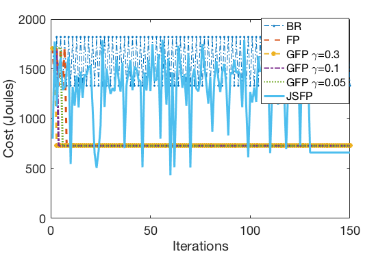
Figure 2: Team’s cost for the first case.

Figure 2 depicts the results for the first case. Best Response failed to converged to an acceptable action, when the other algorithms except Joint strategy fictitious play converged in less than 20 iterations in a solution. All the variants of Geometric fictitious play and the classic fictitious play algorithm were giving as a solution the one with the worst possible cost, 728.7 Joules. On the other hand Joint strategy fictitious play even if it needed more iterations in order to converge to a solution, it provided one with cost of 660.7 Joules. The relative difference between the best possible solution and the one of Joint strategy fictitious play was 25.3%. The relative change is defined as:

$$\Delta=\frac{|x-y|}{\max(x,y)}.$$

.

In the second case robots could visit up to three sensors. Thus, the action space has been increased to 41 possible actions per robot. In addition to the actions, available to each robot in the second case, the action space includes all the possible combinations of visiting three sensors.

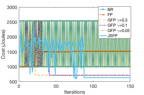
Figure 3: Team’s cost for the third case.

As it is depicted in Figure 3 GFP with $\gamma=0.05$, Fictitious play and Best response fails to converge to a solution. The remaining two instances of Geometric fictitious play converge to the same solution with cost $716.4$ Joules, which is 31.16% worst than the best possible solution. Joint strategy fictitious play needed more iterations to converge to a solution but its corresponding cost was smaller than the two Geometric Fictitious play instances. In particular its cost was 633.3 Joules, 22.12% worst than the most energy efficient solution.

Samples of the trajectories selected by robots for the two cases are depicted in Figures 4 and 5. The robots are denoted A$1$ through A$3$ and their initial poses are marked as arrows, while the targets are denoted T$1$ through T$4$ and their positions are marked with squares.

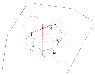
Figure 4: Trajectories of the robots for the first case when Fictitious play algorithm is used.

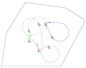
Figure 5: Trajectories of the robots for the second case when Joint strategy fictitious play algorithm is used.

It should be reported that a typical tenfold reduction of time has been observed compared to the classical MILP solver.

VII Conclusions

A game-theoretic formulation for the energy efficient data retrieval problem from stationary nodes using mobile agents is presented. In particular, it is shown that this problem can be cast as a potential game with more than one Nash equilibria. Therefore, a coordination mechanism is needed in order for the robots to reach an acceptable solution. For that reason four basic learning algorithms from game-theoretic literature were used. Even though these algorithms are trapped in local optimum solutions, their computational cost allow them to be utilized in real time applications.

References

- [1] V. Potdar, A. Sharif, and E. Chang, “Wireless sensor networks: A survey,” in International Conference on Advanced Information Networking and Applications Workshops. Bradford, UK: IEEE, May 2009, pp. 636–641.
- [2] D. Bhadauria, O. Tekdas, and V. Isler, “Robotic data mules for collecting data over sparse sensor fields,” Journal of Field Robotics, vol. 28, no. 3, pp. 388–404, 2011.
- [3] O. Tsilomitrou, A. Tzes, and S. Manesis, “Mobile robot trajectory planning for large volume data-muling from wireless sensor nodes,” in 25th Mediterranean Conference on Control and Automation (MED). Valletta, Malta: IEEE, July 2017, pp. 1005–1010.
- [4] A. A. Somasundara, A. Ramamoorthy, and M. B. Srivastava, “Mobile element scheduling for efficient data collection in wireless sensor networks with dynamic deadlines,” in 25th IEEE International Real-Time Systems Symposium. IEEE, December 2004, pp. 296–305.
- [5] D. L. Applegate, R. E. Bixby, V. Chvatal, and W. J. Cook, The traveling salesman problem: A computational study. Princeton University Press, 2011.
- [6] M. Wahab, F. Rios-Gutierrez, and A. E. Shahat, “Energy modeling of differential drive robots,” in SoutheastCon, April 2015, pp. 1–6.
- [7] Y. Mei, Y.-H. Lu, Y. C. Hu, and C. G. Lee, “Energy-efficient motion planning for mobile robots,” in IEEE International Conference on Robotics and Automation (ICRA). New Orleans, LA, USA: IEEE, April 2004, pp. 4344–4349.
- [8] P. Tokekar, N. Karnad, and V. Isler, “Energy-optimal trajectory planning for car-like robots,” Autonomous Robots, vol. 37, no. 3, pp. 279–300, October 2014.
- [9] A. Okabe, B. Boots, and K. Sugihara, “Nearest neighbourhood operations with generalized Voronoi diagrams: A review,” International Journal of Geographical Information Systems, vol. 8, no. 1, pp. 43–71, 1994.
- [10] D. Fudenberg and J. Tirole, Game Theory. Cambridge, MA: MIT Press, 1991.
- [11] J. F. Nash, “Equilibrium points in -person games,” Proceedings of the National Academy of Sciences, vol. 36, no. 1, pp. 48–49, 1950.
- [12] D. Monderer and L. S. Shapley, “Potential games,” Games and Economic Behavior, vol. 14, no. 1, pp. 124–143, 1996.
- [13] D. Fudenberg and D. K. Levine, The theory of learning in games. MIT press, 1998.
- [14] I. Rezek, D. S. Leslie, S. Reece, S. J. Roberts, A. Rogers, R. K. Dash, and N. R. Jennings, “On similarities between inference in game theory and machine learning,” Journal of Artificial Intelligence Research, vol. 33, pp. 259–283, 2008.
- [15] K. Miyasawa, “On the convergence of learning process in a 2x2 non-zero-person game,” 1961.
- [16] J. Robinson, “An iterative method of solving a game,” Annals of Mathematics, vol. 54, no. 2, pp. 296–301, 1951.
- [17] J. Nachbar, ““evolutionary” selection dynamics in games: Convergence and limit properties,” International Journal of Game Theory, vol. 19, pp. 59–89, 1990.
- [18] M. Smyrnakis, H. Qu, and S. M. Veres, “Improving multi-robot coordination by game-theoretic learning algorithms,” International Journal on Artificial Intelligence Tools, vol. 27, no. 07, 2018.