Data assimilation in 2D incompressible Navier-Stokes equations, using a stabilized explicit leapfrog finite difference scheme run backward in time.
Abstract
A stabilized backward marching leapfrog finite difference scheme is applied to hypothetical data at time , to retrieve initial values at time that can evolve into useful approximations to the data at time , even when that data does not correspond to an actual solution. Richardson’s leapfrog scheme is notoriously unconditionally unstable in well-posed, forward, linear dissipative evolution equations. Remarkably, that scheme can be stabilized, marched backward in time, and provide useful reconstructions in an interesting but limited class of ill-posed, time-reversed, 2D incompressible Navier-Stokes initial value problems. Stability is achieved by applying a compensating smoothing operator at each time step to quench the instability. Eventually, this leads to a distortion away from the true solution. This is the stabilization penalty. In many interesting cases, that penalty is sufficiently small to allow for useful results. Effective smoothing operators based on , with real , can be efficiently synthesized using FFT algorithms. Similar stabilizing techniques were successfully applied in several other ill-posed evolution equations. The analysis of numerical stabilty is restricted to a related linear problem. However, as is found in leapfrog computations of well-posed meteorological and oceanic wave propagation problems, such linear stability is necessary but not sufficient in the presence of nonlinearities. Here, likewise, additional Robert-Asselin-Williams (RAW) time-domain filtering must be used to prevent characteristic leapfrog nonlinear instabilty, unrelated to ill-posedness.
Several 2D Navier-Stokes backward reconstruction examples are included, based on the stream function-vorticity formulation, and focusing on pixel images of recognizable objects. Such images, associated with non-smooth underlying intensity data, are used to create severely distorted data at time . Successful backward recovery is shown to be possible at parameter values significantly exceeding expectations.
1 Introduction
This paper discusses the possible use of direct, non iterative, explicit, backward marching finite difference schemes, in data assimilation problems for the 2D incompressible Navier-Stokes equations, at high Reynolds numbers. The actual problem considered here is the ill-posed time-reversed problem of locating appropriate initial values, given hypothetical data at some later time. That problem is emblematic of much current geophysical research activity, using computationally intensive iterative methods based on neural networks coupled with machine learning, [1, 2, 3, 4, 5, 6, 7, 8, 9, 10, 11, 12, 13, 14, 16, 17, 18, 15]. Previous work on backward marching stabilized explicit schemes in 2D nonlinear data assimilation problems, is discussed in [19, 20, 21]. There, it is emphasized that the given hypothetical data at time may not be smooth, may not correspond to an actual solution at time , and may differ from such a solution by an unknown large in an apropriate norm. Moreover, it may not be possible to locate initial values that can evolve into a useful approximation to the desired data at time .
As is well-known, [22, p.59], for ill-posed initial value problems, all consistent stepwise marching schemes, whether explicit or implicit, are necessarily unconditionally unstable and lead to explosive error growth. Nevertheless, it is possible to stabilize such schemes by applying an appropriate compensating smoothing operator at each time step to quench the instability. These schemes then become unconditionally stable, but slightly inconsistent, and lead to distortions away from the true solution. This is the stabilization penalty. In many cases, that penalty is sufficiently small to allow for useful results. Indeed, in [23, 24, 25, 26, 27, 28, 29, 30], backward marching stabilized explicit schemes have been successfully applied to several challenging ill-posed backward recovery problems.
However, such backward recovery problems differ fundamentally from the data assimilation problem considered here. In [23, 24, 25, 26, 27, 28, 29, 30], the given data at time are noisy but relatively smooth, and are known to approximate an actual solution at time , to within a known small in an apropriate norm. While that is not the case in the present data assimilation problem, several computational examples in Section 7 below, will show that success can still be achieved, and on time intervals that are several orders of magnitude larger than might be expected, based on the best-known uncertainty estimates for time-reversed Navier-Stokes equations.
As was the case in [23, 24, 25, 26, 27, 28, 29, 30], the computational examples in Section 7 will be based on pixels gray-scale images, with intensity values that are integers ranging from to . These images represent easily recognizable objects, are defined by highly non-smooth intensity data that would be quite difficult to synthesize mathematically, and they present significant challenges to any ill-posed reconstruction procedure. In addition, images allow for easy visual recognition of possible success or failure in data assimilation.
2 2D Navier-Stokes equations in the unit square
Let be the unit square in with boundary . Let and , respectively denote the scalar product and norm on . We study the 2D problem in stream function-vorticity formulation [31, 32]. Here, the flow is governed by a stream function which defines the velocity components together with the vorticity . The present limited data assimilation study will focus on dissipative properties of Navier-Stokes systems in the absence of active boundary conditions or forcing terms. We restrict attention to stream functions defined on the unit square , which, for the short duration of the flow, vanish together with all their derivatives on and near the boundary . However, will generally have large spatial derivatives away from the boundary. Given such an initial , and a kinematic viscosity , the forward Navier-Stokes initial value problem takes the form
| (1) |
For each , consider the Poisson problem on Let be the solution operator for that problem, so that for , we have We may then rewrite the evolution equation in Eq. (LABEL:eq:0) in the following equivalent form
| (2) |
Solving the system in Eq. (LABEL:eq:0) may be visualized as a marching computation as follows. Given the initial values, the evolution equation for allows advancing forward one time step . The Poisson equation is then solved to obtain , which now allows advancing to the next time step through the evolution equation Eq. (2), and so on.
With the area of the flow domain, define and the Reynolds number as follows
| (3) |
Gray-scale image intensity data have integer values ranging between and . When such images are used to simulate examples of non-smooth stream functions , the primary variables in Eq. (LABEL:eq:0) are derived by taking first and second derivatives of . To prevent very large derivatives and extremely large Reynolds numbers, such intensity values must be rescaled. Premultiplying by , creates an array of non negative numbers ranging from to . This leads to values for and in Eq. (3), that are times smaller than they would otherwise be.
The following example is typical.
2.1 An example: the 2004 Hurricane Ivan stream function
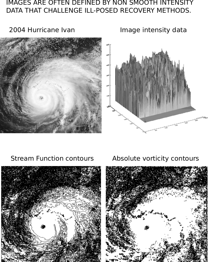
The pixel gray-scale Hurricane Ivan image, and associated intensity data, are shown in Figure 1. The original intensity values were multiplied by , to create an array of non negative numbers ranging from to . We now view as a candidate stream function, defined on the unit square . Contour plots of and of the associated vorticity , are also shown in Figure 1. However, even after reduction by a factor of , one must still expect significant values for the derivatives of . Indeed, with as in Eq. (3), we find
| (4) |
Together with , and in Eq. (3), this leads to a Reynolds number .
In the next section, we imagine the data in Figure 1 to be desired or hypothetical data at some suitable time , and explore the feasibility of reconstructing at from these hypothetical values at time .
3 Uncertainty in backward in time Navier-Stokes reconstruction
In dissipative evolution equations, reconstruction backward in time from imprecise data at some positive time , is an ill-posed continuation problem. With appropriate stabilizing constraints, the uncertainty in such backward continuations is a function of how quickly the given evolution equation forgets the past as time advances. This is explored in such publications as [33, 35, 36, 37, 34, 38, 39, 40], and the references therein. For the Navier-Stokes system in Eq. (LABEL:eq:0), the best-known results are due to Knops and Payne [36, 37], and are based on logarithmic convexity arguments.
In Eq. (LABEL:eq:0), let be the solution on corresponding to approximate data at a given positive time , and let be the unique solution associated with the true data at time . Define on , and on , as follows
| (5) |
For a given small , assume that is small enough that . What constraints must be placed on the solutions of Eq. (LABEL:eq:0) to ensure that will remain small for ? This is the backward stability problem for the Navier-Stokes equations in the norm.
Let be prescribed positive constants. A velocity field is said to belong to the class if
| (6) |
while it belongs to the class if
| (7) |
Define as follows,
| (8) |
If and , it is shown in [36, 37] that then
| (9) |
from which it follows that with ,
| (10) |
A complete derivation for the result in Eq. (10) may be found in [29, Eqs. 9–12].
Let be an a-priori bound for . With , we then obtain
| (11) |
However, as the Hurricane Ivan image in Figure 1 will show, even with very small , need not be small for , because the factor in Eq. (11) may be extremely large, unless is extremely small.
Indeed, with , and the values for given in Eq. (4), we find from Eqs. (6, 7, 8),
| (12) |
With and , we find and . However, with and , we now find and . Thus, in the Hurricane Ivan example in Section 2.1, if , the reconstruction uncertainty at given in Eq. (11), would appear to be too large for any realistic value of the data error at time . We shall revisit that example in the instructive computational experiments described in Section 7 below.
4 Stabilized leapfrog scheme for the 2D Navier-Stokes Equations
Let be the unit square in , and consider the following 2D Navier-Stokes system for
| (13) |
together with the homogeneous boundary conditions
| (14) |
and the initial values
| (15) |
The well-posed forward initial value problem in Eq. (13) becomes ill-posed if the time direction is reversed, and one wishes to recover and from given approximate values for We contemplate both forward and time-reversed computations by allowing for possible negative time steps in the leapfrog time-marching finite difference scheme described below. With a given positive integer , let be the time step magnitude, and let , denote the intended approximation to , and likewise for , and It is helpful to consider Fourier series expansions for , on the unit square ,
| (16) |
with Fourier coefficients given by
| (17) |
With given fixed and , define as follows
| (18) |
For any , let be its Fourier coefficients as in Eq (17). Using Eq. (18), define the linear operators and as follows
| (19) |
As in [23, 24, 25, 26, 27, 28, 29, 30], the operator is used as a stabilizing smoothing operator at each time step. With the operator as in Eq (13), let , and let
| (20) |
Consider the following stabilized leapfrog time-marching difference scheme for the system in Eq (13), in which only the time variable is discretized, while the space variables remain continuous,
| (21) |
The above semi-discrete problem is highly nonlinear. In the operator , the coefficients are ultimately defined in terms of , which is needed to obtain by solving the Poisson problem . The analysis presented in Sections 5 and 6 below, although limited to a related simplified linear problem, is relevant to the above semi-discrete problem. In Section 7, where actual numerical computations are discussed, a uniform grid is imposed on , the space variables are discretized using centered differencing, and FFT algorithms are used to synthesize the smoothing operator . A multigrid algorithm is used to solve the Poisson problem in Eq. (21).
5 Fourier stability analysis in linearized problem
Useful insight into the behavior of the nonlinear scheme in Eq. (21), can be gained by analyzing a related linear problem with constant coefficients. We may naively view in Eq. (15), as a linear operator with time dependent coefficients which need to be evaluated at every time step , through an independent subsidiary calculation. If with positive constants we may study the numerical stability of the system , in Eq. (21), by considering the constant coefficient linear operator , in lieu of . Accordingly, we examine the following evolution equation
| (22) |
together with homogeneous boundary conditions on . With the unique solution in Eq. (22), let
| (23) |
Then, the exact solution satisfies the following leapfrog system
| (24) |
where the truncation error term , is given by
| (25) |
Define the following two component vectors and matrix
| (26) |
| (27) |
One may then rewrite Eq. (24) as
| (28) |
Define norms for two component vectors , and matrices , as follows
| (29) |
Also, for functions on , define the norm as follows
| (30) |
One may also write the stabilized leapfrog scheme for computing Eq. (22) in matrix-vector notation. Let
| (31) |
Then,
| (32) |
With , and matrix defined as
| (33) |
the stabilized marching leapfrog scheme for Eq. (22),
| (34) |
may be written as
| (35) |
Note that with as in Eq. (32),
| (36) |
Unlike the case in Eq. (21), the linear difference scheme in Eq. (35) is susceptible to Fourier analysis. If , then its Fourier coefficients are given by , where
| (37) |
Hence, from Eqs. (18), (19) and (34),
| (38) |
Below, Lemmas 1 and 2, along with Theorems 1 and 2, are stated without proof. Using identical notation, proofs of these results may be found in [30].
Lemma 1
Let be as in Eq. (18), and let be as in Eq. (37). Choose a positive integer such that if , we have
| (39) |
With choose in Eq. (18). Then,
| (40) |
Hence,
| (41) |
and, for ,
| (42) |
Therefore, with this choice of , the linear leapfrog scheme in Eq. (35), is unconditionally stable, marching forward or backward in time.
Proof : See [30, Lemma 5.1]
Lemma 2
Proof : See [30, Lemma 5.2]
With the choice of in Lemma 1,
the stabilized leapfrog scheme in Eq. (35) is unconditionally stable, but at the cost of introducing a small error at each
time step, whose cumulative effect will not vanish as . We now proceed to estimate the error .
Note that Theorems 1 and 2 below refer to the exact solution in Eq. (22), which is a linear diffusion equation with constant coefficients.
Hence, is
necessarily a very smooth function for in each of these Theorems. The same may not be true for the solution of the nonlinear problem in Eq. (13). However,
in [31, 32], highly accurate numerical schemes are advocated for the 2D Navier-Stokes equations.
Such schemes, which presume the existence of high order derivatives, are in common use.
Returning to Eq. (22), the well-posed forward problem, with , is considered first.
Theorem 1
With , let be the unique exact solution of Eq. (22) at . With be as in Lemma 1, let and let . Let be as in Eq. (28), let be the solution of the forward leapfrog scheme in Eq. (35), and let be the constant defined in Eq. (45). If denotes the error at we have, with the norm definitions in Eq. (30)
| (46) |
Hence, as ,
| (47) |
Proof : See [30, Theorem 5.1]
Remark 1.
The first term on the right hand side in Eq. (47) allows for the possibility of erroneous initial data, leading to a positive
value for . The second term is the stabilization penalty, which is the price that must be paid for using the leapfrog scheme in the computation
of the well-posed forward linear problem in Eq. (22). Without stabilization, the leapfrog scheme is unconditionally unstable for that forward problem, and no
error bound would be possible.
As is evident from the discussion in Section 3, small values of must necessarily
be contemplated in Navier-Stokes problems. For an important class of such problems with small and large , the value
of , for some with , may be sufficiently small to allow for useful computations. As an example,
with , we find
.
In the ill-posed backward problem, we contemplate marching backward in time from , using negative time time steps . However, the needed initial data , where is the unique exact solution in Eq. (22), may not be known exactly. For this reason, the ill-posed backward problem is formulated as follows:
With , hypothetical data are given which are assumed to approximate the true data , while approximates true data , both in the norm. Moreover, the unique true backward solution corresponding to the unknown exact data , is such that both and satisfy bounds. Specifically, for some unknown , and some ,
| (48) |
Analogously to the well-posed forward problem in Eq. (35), we now choose and consider the stabilized leapfrog scheme marching backward from with the given hypothetical data in Eq. (48)
| (49) |
where, with as in Eq. (48), and as in Eq. (28), the true solution satisfies
| (50) |
Theorem 2
With as in Eq. (48), and let be the exact solution of the backward problem in Eq. (50) at time With as in Lemma 1, let in the smoothing operator in Eq. (18). Let be the corresponding solution of the stabilized backward leapfrog scheme in Eq. (49), let be the constant in Eq. (45), and let denote the error at time . Then, for with the norm definitions in Eq. (30)
| (51) | |||||
Hence, as ,
| (52) | |||||
Proof : See [30, Theorem 5.2]
Remark 2. As was the case in Eq. (47), there is an additional error term, ,
in Eq. (52).
That term represents the necessary uncertainty in backward reconstruction from possibly erroneous data at time in Eq. (22).
5.1 Application to data assimilation
In Theorems 1 and 2 above, define the constants through as follows, and consider the values shown in Table 1 below.
| (53) | |||||
TABLE 1
Values of through in Eq. (53), with following parameter values:
.
As outlined in the Introduction, data assimilation applied to the system in Eq. (13), is the problem of finding initial values , at , that can evolve into useful approximations to the given hypothetical data at time , as defined by in Eq. (49) in the present linearized problem. If the true solution in Eq. (22) does not have exceedingly large values for and , the parameter values chosen in Table 1, together with Theorem 2, indicate that marching backward to time from the hypothetical data at time , leads to an error at , satisfying
| (54) |
with the constant defined in Eq. (53) presumed small. Next, from Theorem 1, marching forward to time , using the inexact computed initial values, leads to an error at time , satisfying
| (55) |
The error in Theorem 1 is the difference at time , between the unknown unique solution in Eq. (22), and the computed numerical approximation to it provided by the stabilized forward explicit scheme. However, that unknown solution at time differs from the given hypothetical data at time , by an unknown amount in the norm. Hence the total error is
| (56) |
Therefore, data assimilation is successful only if the inexact computed initial values lead to a sufficiently small right hand side in Eq.(56). Clearly, the value of , together with the unknown value of , will play a vital role. As was the case in the nonlinear Knops-Payne uncertainty estimate following Eq. (12) in Section 3, increasing by a factor of ten may not be feasible, even in the simplified linearized problem considered in Table 1. The value of the term in Eq.(56), would increase from to about .
6 Leapfrog nonlinear computational instability and the RAW filter
The results in Theorems 1 and 2 indicate that the stabilizing approach in Eqs. (35) and (49), is sound for the leapfrog scheme applied to the linearized problem. However, for the leapfrog scheme, linear stability is necessary but not always sufficient in the presence of nonlinearities. Leapfrog centered time differencing has been a mainstay of geophysical fluid dynamics computations. In well-posed linear wave propagation problems, a Courant condition is required for leapfrog computational stability. However, even when that Courant condition is obeyed, serious instability can develop in nonlinear problems. This phenomenon, first reported in [41], was subsequently explored and analyzed in [42, 43], and the references therein. Following [41, 42, 43], effective post processing time domain filtering techniques, that can prevent nonlinear instability, were developed in [44, 45, 46, 47, 48]. Such filtering is applied at every time step, and consists of replacing the computed solution with a specific linear combination of computations at previous time steps. These filtering techniques can also be usefully applied in the present 2D Navier-Stokes leapfrog computational problem.
We first describe the Robert-Asselin-Williams filter (RAW), [45, 46], as it applies to the stabilized leapfrog scheme for the forward nonlinear problem with previously considered in Eq. (21). With , and
| (57) |
this forward problem is defined by
| (58) |
For , the forward problem is now modified as follows. With positive constants , where and , and with
| (59) |
with the filtered arrays overwriting the unfiltered arrays at each time step.
With given data for satisfying Eq. (48), and , with the backward
problem is modified in exactly the same way.
The recommended value in [45] is designed to maintain the accuracy in the leapfrog scheme.
Remark 3.
Prior information about the solution is essential in ill-posed inverse problems. While accurate values for and in Eq. (48)
are seldom known, interactive adjustment of the parameter pair in Eqs. (18, 19) in the smoothing operator , often leads to useful reconstructions.
This process is similar to the manual tuning of an FM station, or the manual focusing of binoculars, and likewise requires user recognition of a correct solution.
Beginning with small values of and , chosen so as not to oversmooth the solution, a small number of successive trial reconstructions
are performed. Because of the underlying explicit marching difference scheme, this can be accomplished in a relatively short time. The values of are increased slowly
if instability is detected, and are likewise decreased slowly to increase sharpness, provided no instability results. As is the case with binoculars, useful results are
generally obtained after relatively few trials.
There may be several possible good solutions. Typical values of lie in the ranges .
7 Nonlinear computational experiments
The stabilized leapfrog scheme, together with RAW filtering, can be successfully applied to the full 2D nonlinear Navier-Stokes equations. The computation proceeds along the lines outlined in Section 4. At each time step, a multigrid algorithm is applied to the Poisson problem , with computed at the previous time step. Centered space finite differencing is then applied to to obtain , and to obtain at the next time step by solving the diffusion equation.
In each of Figures 2 through 5 below, the leftmost column presents a single preselected stream function image, as the same hypothetical data at three distinct increasing values of . The middle column presents the corresponding initial value image at , computed by the backward marching stabilized leapfrog scheme. Finally, the rightmost column, presents the forward evolution to time , of the previously computed initial value image immediately to the left.
Evidently, given the same hypothetical stream function data, assimilation becomes less successful with increasing preselected . The first row in each of Figures 2 through 5, is considered a successful example of 2D Navier-Stokes data assimilation. For each first row, the corresponding behavior of the norms for each of and , in the assimilation process, is described in Tables 2 through 5. An important phenomenon is immediately noticeable in each of these tables. The norm of the evolved stream function at time , in the rightmost image in each first row, is a close approximation to that in the hypothetical stream function in the leftmost image in that same first row. However, the norms of the derivatives of in the evolved image at time in each first row, are substantially smaller than the corresponding norms in the leftmost hypothetical data image. This can be explained by the fact that the evolved image at time is a computed solution to the 2D Navier-Stokes equations. Such a solution would necessarily be a smooth approximation to hypothetical data that might be far from an actual solution at the same time Indeed, Figure 6 shows how the stream function data , in the first row hypothetical and evolved Hurricane Ivan images, actually compare. The approximating evolved data on the right, are noticeably smoother than the hypothetical data on the left.
Finally, it is noteworthy that successful assimilation from a value on the order of , was found possible in the Hurricane Ivan image, given the uncertainty estimates following Eq. (12) in Section 3. These estimates indicated a necessary value for on the order of . However, rigorous uncertainty estimates must necessarily contemplate worse case error accumulation scenarios, and may be too pessimistic in individual cases. The other examples in Tables 2, 3 and 5, also involve significantly larger values than might be anticipated.
8 Concluding Remarks
Along with [19, 20, 21], the results in the present paper invite useful scientific debate and comparisons, as to whether equally good or better results might be achieved using the computational methods described in [1, 2, 3, 4, 5, 6, 7, 8, 9, 10, 11, 12, 13, 14, 16, 17, 18, 15]. As an alternative computational approach, backward marching stabilized explicit schemes may also be helpful in verifying the validity of suspected hallucinations in computations involving machine learning.
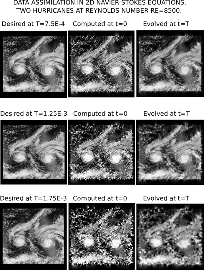
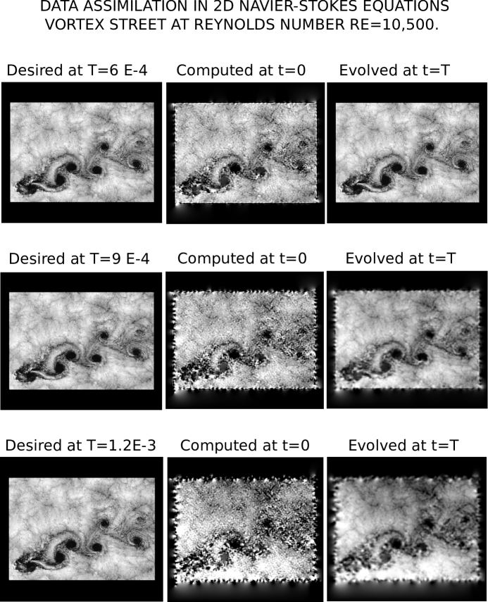
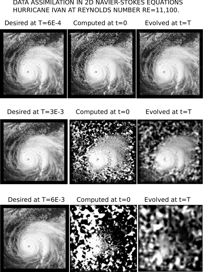
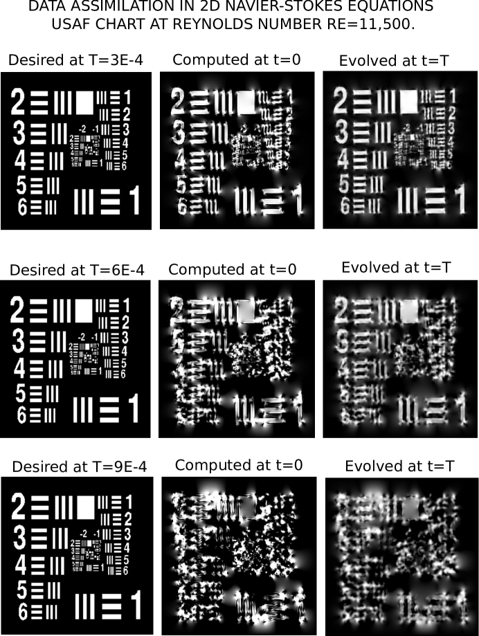
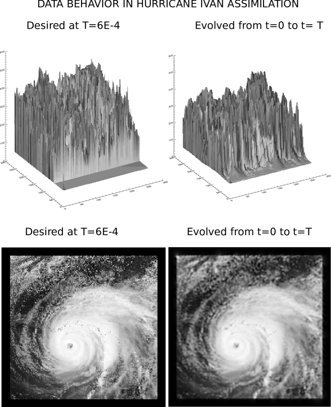
TABLE 2
Two Hurricanes image at
-norm behavior in data assimilation from hypothetical data at
| Variable | Desired at norm | Computed at norm | Evolved at norm |
|---|---|---|---|
| 0.294 | 0.308 | 0.288 | |
| 12.3 | 20.6 | 8.5 | |
| 12.7 | 20.4 | 8.8 | |
| 14301 | 13986 | 3951 |
TABLE 3
Vortex Street image at RE=10,500
-norm behavior in data assimilation from hypothetical data at
| Variable | Desired at norm | Computed at norm | Evolved at norm |
| 0.352 | 0.351 | 0.341 | |
| 10.0 | 14.1 | 7.3 | |
| 10.7 | 15.0 | 7.9 | |
| 10815 | 9579 | 3492 |
TABLE 4
Hurricane Ivan image at RE=11,100
-norm behavior in data assimilation from hypothetical data at
| Variable | Desired at norm | Computed at norm | Evolved at norm |
|---|---|---|---|
| 0.356 | 0.362 | 0.350 | |
| 13.32 | 18.21 | 8.46 | |
| 12.89 | 17.74 | 7.87 | |
| 18094 | 13207 | 4426 |
TABLE 5
USAF Chart image at RE=11,500
-norm behavior in data assimilation from hypothetical data at
| Variable | Desired at norm | Computed at norm | Evolved at norm |
|---|---|---|---|
| 0.263 | 0.300 | 0.245 | |
| 23.62 | 27.75 | 16.93 | |
| 21.17 | 25.25 | 15.19 | |
| 15916 | 15110 | 7695 |
References
- [1] Cintra R, de Campos Velho HF, Cocke S. Tracking the model: data assimilation by artificial neural network. 2016 International Joint Conference on Neural Networks (IJCNN), Vancouver, BC, Canada. 2016:403-410. DOI:10.1109/IJCNN.2016.7727227.
- [2] Howard LJ, Subramanian A, Hoteit I. A machine learning augmented data assimilation method for high resolution observations. Journal of Advances in Modeling Earth Systems. 2024;16,e2023MS003774. https://doi.org/10.1029/2023MS003774.
- [3] Blum J, Le Dimet F-X, Navon I-M. Data Assimilation for Geophysical Fluids. Handbook of Numerical Analysis. 2009;14:385-441. https://doi.org/10.1016/S1570-8659(08)00209-3
- [4] He Q, Barajas-Solano D, Tartakovsky G, et al. Physics-informed neural networks for multiphysics data assimilation with application to subsurface transport. Advances in Water Resources 2020; https://doi.org/10.1016/j.advwatres.2020.103610.
- [5] Arcucci R, Zhu J, Hu S, et al. Deep data assimilation: integrating deep learning with data assimilation. Appl. Sci. 2021;11:1114. https://doi.org/10.3390/app11031114.
- [6] Antil H, Lohner R, Price R. Data assimilation with deep neural nets informed by nudging. https://arxiv.org/abs/2111.11505. November 2021.
- [7] Chen C, Dou Y, Chen J, et al. A novel neural network training framework with data assimilation. Journal of Supercomputing. 2022;78:19020–19045. https://doi.org/10.1007/s11227-04629-7
- [8] Lundvall J, Kozlov V, Weinerfelt P. Iterative methods for data assimilation for Burgers’ equation. J. Inverse Ill-Posed Probl. 2006;14:505–535.
- [9] Auroux D, Blum J. A nudging-based data assimilation method for oceanographuc problems: the back and forth nudging (BFN) algorithm. Proc. Geophys. 2008;15:305–319.
- [10] Ou K, Jameson A. Unsteady adjoint method for the optimal control of advection and Burgers’ equation using high order spectral difference method. 49th AIAA Aerospace Science Meeting, 4-7 January 2011. Orlando, Florida.
- [11] Auroux D, Nodet M. The back and forth nudging algorithm for data assimilation problems: theoretical results on transport equations. ESAIM:COCV 2012;18:318–342.
- [12] Auroux D, Bansart P, Blum J. An evolution of the back and forth nudging for geophysical data assimilation: application to Burgers equation and comparison. Inverse Probl. Sci. Eng. 2013;21:399-419
- [13] Allahverdi N, Pozo A, Zuazua E. Numerical aspects of large-time optimal control of Burgers’ equation. ESAIM Mathematical Modeling and Numerical Analysis 2016;50:1371–1401.
- [14] Gosse L, Zuazua E. Filtered gradient algorithms for inverse design problems of one-dimensional Burgers’ equation. Innovative Algorithms and Analysis 2017;197–227.
- [15] de Campos Velho HF, Barbosa VCF, Cocke S. Special issue on inverse problems in geosciences. Inverse Probl. Sci. Eng. 2013;21:355-356. DOI:10.1080/17415977.2012.712532
- [16] Gomez-Hernandez JJ, Xu T. Contaminant source identification in acquifers: a critical view. Math Geosci 2022;54:437–458.
- [17] Xu T, Zhang W, Gomez-Hernandez JJ, et al. Non-point contaminant source identification in an acquifer using the ensemble smoother with multiple data assimilation. Journal of Hydrology 2022; 606:127405.
- [18] Vukicevic T, Steyskal M, Hecht M. Properties of advection algorithms in the context of variational data assimilation. Monthly Weather Review 2001;129:1221–1231.
- [19] Carasso AS. Data assimilation in 2D viscous Burgers equation using a stabilized explicit finite difference scheme run backward in time. Inverse Probl. Sci. Eng. 2021;29:3475–3489. DOI:10.1080/17415977.2021.200947
- [20] Carasso AS. Data assimilation in 2D nonlinear advection diffusion equations, using an explicit stabilized leapfrog scheme run backwrd in time. NIST Technical Note 2227, July 12 2022. DOI:10.6028/NIST.TN2227
- [21] Carasso AS. Data assimilation in 2D hyperbolic/parabolic systems using a stabilized explicit finite difference scheme run backward in time. Applied Mathematics in Science and Engineering, 2024;32:1,228641. DOI:10.1080/27690911.2023.228641
- [22] Richtmyer RD, Morton KW. Difference Methods for Initial Value Problems. 2nd ed. New York (NY): Wiley; 1967
- [23] Carasso AS. Compensating operators and stable backward in time marching in nonlinear parabolic equations. Int J Geomath 2014;5:1–16.
- [24] Carasso AS. Stable explicit time-marching in well-posed or ill-posed nonlinear parabolic equations. Inverse Probl. Sci. Eng. 2016;24:1364–1384.
- [25] Carasso AS. Stable explicit marching scheme in ill-posed time-reversed viscous wave equations. Inverse Probl. Sci. Eng. 2016;24:1454–1474.
- [26] Carasso AS. Stabilized Richardson leapfrog scheme in explicit stepwise computation of forward or backward nonlinear parabolic equations. Inverse Probl. Sci. Eng. 2017;25:1–24.
- [27] Carasso AS. Stabilized backward in time explicit marching schemes in the numerical computation of ill-posed time-reversed hyperbolic/parabolic systems. Inverse Probl. Sci. Eng. 2018;1:1–32. DOI:10.1080/17415977.2018.1446952
- [28] Carasso AS. Stable explicit stepwise marching scheme in ill- posed time-reversed 2D Burgers’ equation. Inverse Probl. Sci. Eng. 2018;27(12):1-17. DOI:10.1080/17415977.2018.1523905
- [29] Carasso AS. Computing ill-posed time-reversed 2D Navier-Stokes equations, using a stabilized explicit finite difference scheme marching backward in time. Inverse Probl. Sci. Eng. 2019; DOI:10.1080/17415977.2019.1698564
- [30] Carasso AS. Stabilized leapfrog scheme run backward in time, and the explicit stepwise computation of ill-posed time-reversed 2D Navier-Stokes equations. Inverse Probl. Sci. Eng. 2021; DOI:10.1080/17415977.2021.1972997
- [31] Johnston H, Liu JG. Finite difference schemes for incompressible flow based on local pressure boundary conditions. J. Comput. Phys. 2002;180:120–154.
- [32] Ghadimi P, Dashtimanesh A. Solution of 2D Navier-Stokes equation by coupled finite difference-dual reciprocity boundary element method. Applied Mathematical Modelling 2011;35:2110–2121.
- [33] Ames KA, Straughan B. Non-Standard and Improperly Posed Problems. New York (NY): Academic Press; 1997.
- [34] Payne LE. Some remarks on ill-posed problems for viscous fluids. Int. J. Engng Sci. 1992;30:1341–1347.
- [35] Knops RJ. Logarithmic convexity and other techniques applied to problems in continuum mechanics. In: Knops RJ, editor. Symposium on non-well-posed problems and logarithmic convexity. Vol. 316, Lecture notes in mathematics. New York (NY): Springer-Verlag; 1973.
- [36] Knops RJ, Payne LE. On the stability of solutions of the Navier-Stokes equations backward in time. Arch. Rat. Mech. Anal. 1968;29:331–335.
- [37] Payne LE. Uniqueness and continuous dependence criteria for the Navier-Stokes equations. Rocky Mountain J. Math. 1971;2:641–660.
- [38] Carasso AS. Reconstructing the past from imprecise knowledge of the present: Effective non-uniqueness in solving parabolic equations backward in time. Math. Methods Appl. Sci. 2012;36:249-–261.
- [39] Carasso A. Computing small solutions of Burgers’ equation backwards in time. J. Math. Anal. App. 1977;59:169–209.
- [40] Hào DN, Nguyen VD, Nguyen VT. Stability estimates for Burgers-type equations backward in time. J. Inverse Ill Posed Probl. 2015;23:41–49.
- [41] Phillips NA. An example of non-linear computational instability. In: Bolin B. editor, The Atmosphere and the Sea in Motion. Rockefeller Institute; New York (NY) 1959. p. 501-504.
- [42] Fornberg B. On the instability of Leapfrog and Crank-Nicolson approximations of a nonlinear partial differential equation. Math Comput. 1973;27:45-57.
- [43] Sanz-Serna JM. Studies in numerical nonlinear instability I. Why do leapfrog schemes go unstable ? SIAM J. Sci. Stat. Comput. 1985;6:923-938.
- [44] Asselin R. Frequency filter for time integrations. Mon Weather Rev. 1972;100:487-490.
- [45] Williams PD. A proposed modification to the Robert-Asselin time filter. Mon Weather Rev. 2009;137:2538-2546.
- [46] Williams PD. The RAW filter: An improvement to the Robert-Asselin filter in semi-implicit integrations. Mon Weather Rev. 2011;139:1996-2007.
- [47] Amezcua J, Kalnay E, Williams PD. The effects of the RAW filter on the climatology and forecast skill of the SPEEDY model. Mon Weather Rev. 2011;139:608-619.
- [48] Hurl N, Layton W, Li Y, et al. Stability analysis of the Crank-Nicolson-Leapfrog method with the Robert-Asselin-Williams time filter. BIT Numer Math. 2014;54:1009-1021.