Limits of the Lindblad and non-Hermitian description of open systems

Abstract

While it is well established that the dynamics of an open system is described well by the Lindblad master equation if the coupling to the bath is either in the weak or in the singular limit, it is not known whether this description can be extended to some other coupling strength. Here we use the exact solution of a microscopic system coupled to baths, to show that, for a pure decay system, Lindbladian dynamics only holds in the weak and singular coupling limits. We also show that Lindblad and non-Hermitian dynamics are equivalent in the highest particle subspace of such systems with pure decay. Using this equivalence, we rule out the possibility of obtaining non-Hermitian dynamics for any other couplings. Furthermore, we argue that exceptional points can only occur in the singular coupling limit, never in the weak coupling limit. Physically, this means that exceptional points can occur when the intrinsic time evolution of the isolated system is comparable to the relaxation time scale.

Introduction: A great challenge of modern physics is to identify and understand the novel quantum phenomena that occur in open systems [1, 2]. This requires a good understanding of the theoretical frameworks that can be used to accurately describe experimental data [3, 4, 5, 6, 7]. Therefore, an important theoretical goal is to study how to properly ‘integrate out’ the large number of degrees of freedom in a bath model.

One well established approach for modelling open systems is the Lindblad Master equation [8, 9, 10], which replaces solving the Schrödinger equation for the total Hamiltonian

$$H=H_{A}+H_{B}+H_{C}$$ (1)

where $H_{A}$, $H_{B}$ and $H_{C}$ describe the system, the bath, and their coupling, respectively, with the Lindblad equation for the density matrix of the system

$$\dot{\rho}_{A}=\mathcal{L}[\rho_{A}]=-\text{i}[H_{A},\rho_{A}]\\ +\sum_{j}\Gamma_{j}\left(L_{j}\rho_{A}L_{j}^{\dagger}-\frac{1}{2}\left\{L_{j}^{\dagger}L_{j},\rho_{A}\right\}\right).$$ (2)

Here $L_{j}$ are system operators, the gain/decay rates $\Gamma_{j}$ vanish when $H_{C}=0$, and we set $\hbar=1$.

The Lindblad Master equation assumes a Markovian bath and was proven to be accurate (i) in the weak coupling limit, where the energy scale $C$ of the system-bath coupling is much smaller than the energy scales $A,B$ of the system and of the bath; and (ii) in the singular limit where $B/A\rightarrow\infty$ and $C/A\rightarrow\infty$ such that $C^{2}/B$ is constant [1, 11]. The Lindblad approach was found to work reasonably well for interpreting experiments [3, 4, 5, 6, 7], but it remains an open question whether it is generically accurate outside the two limits mentioned above.

Another very popular approach for the study of open systems is to assume that the dynamical equation for $\rho_{A}$ is like the first line of Eq. (2), i.e. like that of a closed system, but with the system Hamiltonian $H_{A}$ replaced by some non-Hermitian operator $H_{nh}$ [12, 13, 14, 15, 16, 17]. However, it is still far from clear when such a non-Hermitian description of an open system is adequate.

A direct link between the two approaches is established by noting that if the action of the quantum jumps term

$$\mathcal{Q}[\rho_{A}]=\sum_{j}\Gamma_{j}L_{j}\rho_{A}L_{j}^{\dagger}$$ (3)

can be ignored in Eq. (2), then the Lindblad equation is equivalent to evolution under the non-Hermitian operator [18, 19]

$$H_{\text{nh}}=H_{A}-\frac{\text{i}}{2}\sum_{j}\Gamma_{j}{L}^{\dagger}_{j}L_{j}.$$ (4)

The right eigenvectors of this non-Hermitian operator are not necessarily orthogonal to one another. This can lead to exceptional points where two eigenvectors of $H_{\text{nh}}$ become parallel to one another [20, 18, 19, 3, 21].

The first major result of this Letter is to demonstrate that for pure decay systems (defined below), the Lindblad approximation is not valid outside the weak and singular coupling limits. For brevity, we will refer to this as R1. A second result of our work (R2) is to prove that for Lindblad dynamics with pure decay, quantum jumps can be ignored in the subspace with the highest particle number. This provides an exact equivalence between Lindblad dynamics and non-Hermitian dynamics. Our third major result (R3) is to demonstrate that for pure decay systems, exceptional points can exist only in the singular coupling limit and not in the weak coupling limit. This means that the intrinsic timescale of the isolated system must be comparable to the relaxation time of the system. This result will help guide experimental searches for open systems with exceptional points.

Pure decay system: consider a system which initially has $N$ particles, and which is connected to an empty bath at time $t=0$. If the bath modelling is appropriate for the system, i.e. all the eigenstates of the isolated system overlap with the bath spectrum, then the number of particles in the system vanishes as $t\rightarrow\infty$. We call such an open system, and any other system that can be mapped onto it, a pure decay system.

Let ${\cal H}_{N}$ be the $N$-particle Hilbert space of the system, and let $\rho_{N}:{\cal H}_{N}\rightarrow{\cal H}_{N}$ be the component of the system’s density matrix $\rho_{A}(t)$ that describes the evolution purely within this highest number of particles subspace. If the evolution of $\rho_{A}(t)$ is Lindbladian, then the evolution of $\rho_{N}(t)$ is non-Hermitian:

$$\rho_{N}(t)=\exp(-\text{i}H_{\text{nh}}t)\rho_{N}(0)\exp(\text{i}H_{\text{nh}}^{\dagger}t)$$ (5)

where $H_{nh}$ is given by Eq. 4. This is R2, and holds because $\mathcal{Q}[\rho_{N}]=0$, i.e. the quantum jumps have no effect within this particular subspace. Of course, the quantum jumps are essential for evolving $\rho_{A}$ into subspaces with fewer than $N$ particles, so the full evolution of $\rho_{A}(t)$ need not be non-Hermitian.

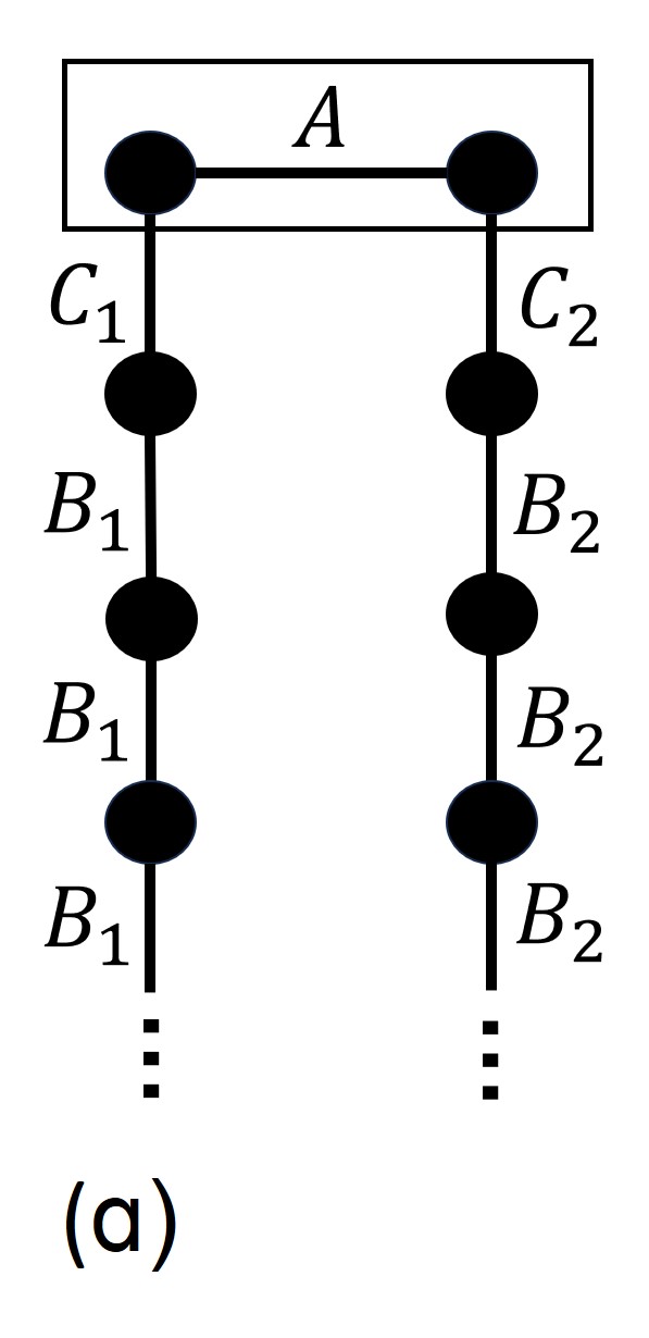
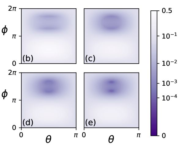
Figure 1: ($a$) Sketch of the system+bath model considered here. ($b$)-($e$) $R_{\theta,\phi}$ of Eq. (7) as a function of $\theta$ and $\phi$ for $C_{1}=C$, $C_{2}=3C$, $B_{1}=B$, $B_{2}=2B$ and $\frac{C^{2}}{B}=0.5$, and ($b$) $B=2$, $C=1$, ($c$) $B=4$, $C=\sqrt{2}$, ($d$) $B=8$, $C=2$ and ($e$) $B=16$, $C=2\sqrt{2}$. As the singular limit is approached, the two minima approach zero, validating non-Hermitian dynamics in this limit.

If we are able to solve the system+bath evolution exactly, we can verify whether the evolution of $\rho_{N}(t)$ is non-Hermitian as follows. We begin by assuming that there is a non-Hermitian $H_{nh}$ such that $\rho_{N}(t)$ is given by Eq. (5), and let $|v\rangle$ be a right eigenvector of $H_{nh}$. If we choose $|v\rangle$ as the initial state then $\rho_{N}(t)\propto|v\rangle\langle v|$ (with a decaying pre-factor) for all times, i.e. this initial state does not mix into other $N$-particle states. Explicitly, if $P_{v}=1-|v\rangle\langle v|$ is the projector onto $N$-particle states orthogonal to $|v\rangle$, then

$$r_{v}(t)=\Tr[\rho_{N}(t)P_{v}]=0$$ (6)

at all times.

For completeness, is important to note that the reciprocal is not necessarily true, i.e. it is possible to find vectors for which $r_{v}(t)=0$ when $\rho_{N}(t)$ is not described by non-Hermitian dynamics. This can happen when there are additional global symmetries of the system+bath total Hamiltonian, which protect subspaces invariant to these symmetries from mixing. We presume that such symmetries would be broken in a realistic system with any degree of imperfections, whereas if $r_{v}(t)=0$ arises from non-Hermitian dynamics, it should be more robust to such imperfections (lack of global symmetries).

To summarize, we can find possible right eigenvectors of $H_{nh}$ –and thus, confirm that the evolution of $\rho_{N}(t)$ is indeed non-Hermitian if the system does not have global symmetries– by scanning through all states $|v\rangle$ in the $N$-particle subspace, and finding all non-mixing states satisfying Eq. (6). In the following, we use its reciprocal: if there are no initial states that satisfy Eq. (6), the evolution of $\rho_{N}(t)$ cannot be non-Hermitian.

Next, we use an exact solution for a pure decay systen to show that the evolution of $\rho_{N}(t)$ is non-Hermitian only in the weak- and singular-coupling limits. Combined with R2, this means that the evolution of $\rho_{A}(t)$ cannot be Lindbladian away from these limits, thus proving R1.

Model and methods: Pure decay system+bath problems can be evolved exactly from any initial state for any $N$, although the computational costs quickly become prohibitive. We consider here an example with $N=1$, which suffices for our purposes. The model is sketched in Fig. 1a, and consists of a two-site system $H_{A}=A(a_{1}^{\dagger}a_{2}+a_{2}^{\dagger}a_{1})$, where $a_{s}^{\dagger}|0\rangle$ has a particle at site $s=1,2$. Each site is coupled to its own bath, described by semi-infinite chains $H_{B}=\sum_{s=1}^{2}B_{s}\sum_{j=1}^{\infty}\left(b_{s,j}^{\dagger}b_{s,j+1}+b_{s,j+1}^{\dagger}b_{s,j}\right)$ that allow particles to move inside the respective $s=1,2$ bath [22, 23]. Finally, the coupling is $H_{C}=\sum_{s=1}^{2}C_{s}\left(a_{s}^{\dagger}b_{s,1}+b_{s,1}^{\dagger}a_{s}\right)$. We use standard Green’s functions methods [22] (details in the appendix) to calculate the time evolution of all $N=1$ initial states parameterized as $|v\rangle=|\theta,\phi\rangle=(\cos\theta a_{1}^{\dagger}+e^{\text{i}\phi}\sin\theta a_{2}^{\dagger})|0\rangle$. Because this $N=1$ Hilbert space has dimension $d=2$, the projector $P_{v}=1-|v\rangle\langle v|=|{\bar{\theta}},{\bar{\phi}}\rangle\langle{\bar{\theta}},{\bar{\phi}}|$, where $|{\bar{\theta}},{\bar{\phi}}\rangle=(-e^{-\text{i}\phi}\sin\theta a_{1}^{\dagger}+\cos\theta a_{2}^{\dagger})|0\rangle$ is the 1-particle state orthonormal to $|v\rangle$. Thus, for any set values of $A,B_{s},C_{s}$, we can scan the $\theta,\phi$ space and calculate

$$R_{\theta,\phi}=\max_{t}|r_{v}(t)|$$ (7)

where $|v\rangle=|\theta,\phi\rangle$, over a finite time interval.

The symmetric case with $C_{1}=C_{2}$ and $B_{1}=B_{2}$ has a global inversion symmetry, and thus the states $|v_{\pm}\rangle=\frac{1}{\sqrt{2}}(a_{1}^{\dagger}\pm a_{2}^{\dagger})|0\rangle$ do not mix, resulting in $R_{\theta,\phi}=0$ for $\theta=\pi/2$ and $\phi=0,\pi$ strictly because of symmetry, irrespective of the nature of the underlying dynamics. As mentioned, we ignore such a ’perfect’ model, which is unlikely to be realized in practice.

Instead, we consider a non-symmetric case with $C_{2}=3C_{1}=3C$, and $B_{2}=2B_{1}=2B$ (similar results are found for any other non-unity ratios). Next, we ask for which parameters $H_{B}$ acts as a valid bath for the system. For our choices, the spectrum of $H_{B}$ ranges over $[-4B,4B]$ while the spectrum of $H_{A}$ has eigenergies at $-A$ and $A$. So, intuitively, if $4B<A$, then a particle could remain trapped at all times in the subsystem $A$, depending on the initial state (i.e. the bath model is not appropriate). This intuition is correct, but a more accurate valid-baths condition involves both $b_{A}=B/A$ and $c_{A}=C/A$:

$$c_{A}^{2}<\frac{2b_{A}^{2}(x_{0}+y_{0})-\sqrt{4b_{A}^{4}(x_{0}-y_{0})^{2}+x_{0}y_{0}b_{A}^{2}}}{x_{0}y_{0}}.$$ (8)

where $x_{0}=1/(2+\sqrt{3})$ and $y_{0}=9/2$ (see the appendix for a derivation).

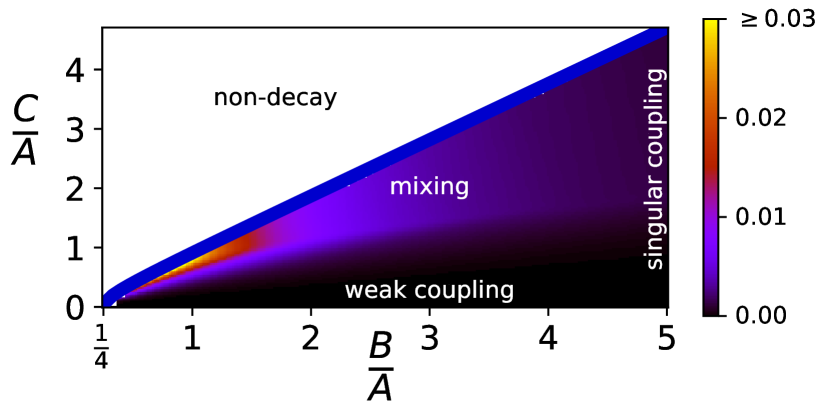
Figure 2: The mixing parameter $\mathcal{R}$ of Eq. (9) when $C_{1}=C$, $C_{2}=3C$, $B_{1}=B$, $B_{2}=2B$. The blue line separating the decay and non-decay regions is Eq. (8). In the decay region, possible non-Hermitian dynamics signalled by $\mathcal{R}\rightarrow 0$ (dark regions) is observed only in the weak coupling region (bottom region) and in the singular coupling region (right side).

We thus calculate $R_{\theta,\phi}$ collected over the time interval $0\leq t\leq 4\pi/A$, within the decay region. In Figure 1, we set $\frac{C^{2}}{B}=0.5$ with ($b$) $B=2$, $C=1$, ($c$) $B=4$, $C=\sqrt{2}$, ($d$) $B=8$, $C=2$ and ($e$) $B=16$, $C=2\sqrt{2}$, moving towards the singular coupling limit. The global minima in the subfigures are roughly ($b$) $0.0048$, ($c$) $0.0013$, ($d$) $0.0005$ and ($e$) $0.0001$. In all cases there are two local minima indicating the appearance of two non-mixing states in the singular coupling limit, which is approached asymptotically from panel ($b$) to ($e$).

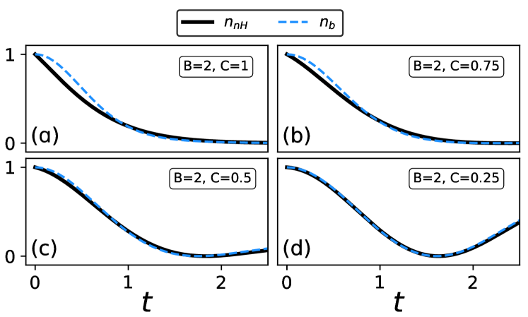
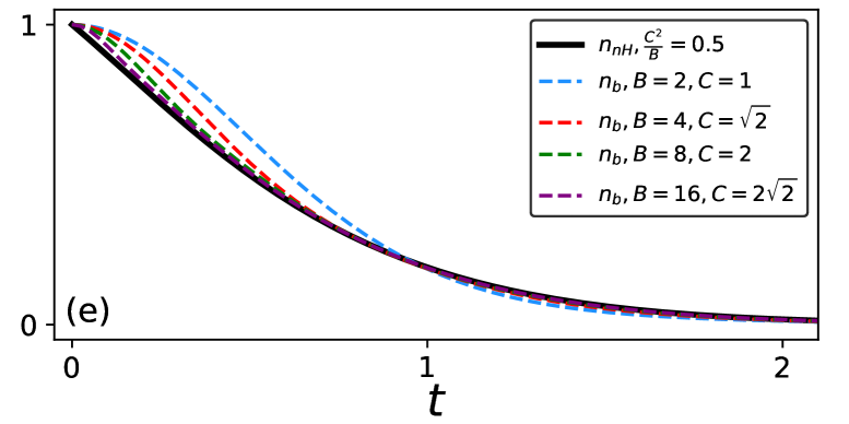
Figure 3: Comparison between $n_{nH}(t)$ and $n_{b}(t)$ as a function of $t$. The plots $(a)$, $(b)$, $(c)$, $(d)$ are approaching the weak coupling limit, showing improved agreement as $C\rightarrow 0$. Plot $(e)$ demonstrates good agreement in the singular coupling limit.

To search for such minima systematically, we use the global parameter

$$\mathcal{R}=\min_{\theta,\phi}R_{\theta,\phi}$$ (9)

to characterize whether the evolution of $\rho_{N}(t)$ is (when $\mathcal{R}=0$) or is not (when $\mathcal{R}>0$) non-Hermitian.

Figure 2 illustrates such an analysis for the same system, i.e. $C_{2}=3C_{1}=3C$, and $B_{2}=2B_{1}=2B$ (similar results are found for any other system without global symmetries). The blue line separates the decay and non-decay regions, where the valid baths condition is and is not obeyed, respectively. The value of $\mathcal{R}$ is shown as a contour plot for the decay region in the $(B/A,C/A)$ parameter space. The plot reveals that $\mathcal{R}\rightarrow 0$ in the bottom region of the plot (the weak coupling limit, $C/A\ll 1$) and in the asymptotic right-side of the plot (the singular coupling limit, $C/A\rightarrow\infty$, $B/A\rightarrow\infty$ with $\gamma=C^{2}/B={\rm const.}$). This confirms that in these limits, the evolution of $\rho_{N=1}(t)$ is non-Hermitian, consistent with the known fact that here, the evolution of $\rho_{A}(t)$ is described well by the Lindblad master equation [1].

$\mathcal{R}$ is finite everywhere else apart from these two asymptotic limits, showing that the evolution of $\rho_{N=1}(t)$ cannot be non-Hermitian, and thus proving that the evolution of $\rho_{A}(t)$ is not captured by the Lindblad master equation anywhere else in the parameter space. Even though this result is established for our simple system+bath model, it rules out the existence of other generic limits (besides the weak coupling and the singular coupling ones) where the evolution is Lindbladian: if they existed, they should hold for our simple model as well and thus be visible in Fig. 2 as other regions where $\mathcal{R}\rightarrow 0$.

Another way to validate this result, is to compare the expectation values of various systems operators $O_{A}$ with those predicted by the Lindblad master equation. For our simple model, ${\cal O}_{A}(t)=\tr[\rho_{A}(t)O_{A}]=\tr[\rho_{N=1}(t)O_{A}]$ for any system operator $O_{A}$ that conserves the particle number, because of the vanishing contribution from the vacuum component $\rho_{N=0}(t)$ of $\rho_{A}(t)$.

As established by R2, Lindbladian evolution for $\rho_{A}(t)$ means non-Hermitian evolution in the $N=1$ subspace. For our simple model, Eq. (4) reads:

$$H_{\text{nh}}=H_{A}-{\text{i}\over 2}\sum_{s=1}^{2}\Gamma_{s}a_{s}^{\dagger}a_{s}$$ (10)

where $\Gamma_{s}=2\frac{C_{s}^{2}}{B_{s}}$. A justification for this is shown in the appendix.

Figure 3 compares the time evolution of the expectation values of the operator $O_{A}=a_{1}^{\dagger}a_{1}$, calculated with the exact system+bath solution (curves labeled $n_{b}$) versus those calculated with the non-Hermitian operator of Eq. (10) (curves labeled $n_{nh})$. In all cases, the initial state is chosen to be $a_{1}^{\dagger}|0\rangle$ and once again we set $C_{2}=3C_{1}=3C$, $B_{2}=2B_{1}=2B$; similar results are found for any other non-unity ratios. Panels $(a)$, $(b)$, $(c)$ and $(d)$ show the results in the weak limit, for fixed $B=2$ and $C$ approaching zero. Panel $(e)$ shows the singular limit with $\frac{C^{2}}{B}=0.5$ fixed and both $B$ and $C$ increasing. As expected, there is good agreement between the exact and the non-Hermitian results as these limits are approached.

Results like those shown in Fig. 3 offer additional support for the validity of R1: the dynamics of $\rho_{N=1}(t)$ approaches non-Hermitian time-evolution asymptotically in the known singular and weak coupling limits. We do not find non-Hermitian evolution of $\rho_{N=1}(t)$ elsewhere, and therefore the evolution of $\rho_{A}(t)$ is not described by the Lindblad master equation (R2), away from the weak- and the singular-coupling limits.

This analysis also allows us to make an important point about the existence of exceptional points. The first condition is that the evolution must be Lindbladian. As already established, for a decay system this means that the system must be either in the weak or in the singular coupling limit. Within these two limits, then, and within the Hilbert space with the largest particle number $N$, tuning to an exceptional point is achieved when at least two right eigenvectors of $H_{nh}$ become identical.

For our simple system+bath model, it is straightforward to check that the right eigenvectors for $H_{nh}$ of Eq. (10) become identical when

$$2A=|\Gamma_{1}-\Gamma_{2}|=\left|\frac{C_{1}^{2}}{B_{1}}-\frac{C_{2}^{2}}{B_{2}}\right|.$$ (11)

The semi-infinite chains act as baths when Eq. (8) is satisfied, i.e. both $B_{s}/A$ ratios are larger than a number of order unity. It is then clear that there cannot be an exceptional point when both baths are in the weak-coupling limit with $C_{s}/A\rightarrow 0$. For example, for our parametrization $C_{2}=3C_{1}=3C$, $B_{2}=2B_{1}=2B$ we find that Eq. (11) holds if $3.5c_{A}^{2}=2b_{A}$. Combining Eqs. (11) and (8), we find that an exceptional point is possible for $b_{A}>0.733$ and $c_{A}>0.647$, well outside the weak coupling limit $c_{A}\rightarrow 0$.

This is also clear on physical grounds: if the couplings to the baths are perturbationally small, to zeroth order the eigenvectors of $H_{nh}$ are equal to the eigenvectors of $H_{A}$. The latter are always orthogonal and therefore distinct, and cannot be made identical by the addition of small perturbative corrections. This argument holds for any system+bath model, not just for our simple example.

Eq. (11) can be interpreted in terms of characteristic timescales. There are three such scales: $\tau_{A}\sim\frac{1}{A}$, $\tau_{B}\sim\frac{1}{B}$ and $\tau_{R}\sim\frac{1}{\Gamma}\sim\frac{B}{C^{2}}$ associated with the intrinsic evolution of the system, of the bath, and the relaxation time of the system because of the coupling to the bath, respectively. (For simplicity, we assume that if there are multiple baths, their energy scales and their couplings, respectively, are roughly equal). Lindbladian dynamics implies a markovian bath satisfying $\tau_{B}\ll\tau_{R}$; this condition is obeyed both in the weak coupling and in the singular coupling limit. Eq. (11) suggests that an exceptional point can be found if additionally $\tau_{A}\sim\tau_{R}$, i.e. when the system timescale and the relaxation time are comparable.

To summarize, a necessary condition for an exceptional point to appear is that the baths coupled to the system must be in the singular limit $B/A\rightarrow\infty$ and $C/A\rightarrow\infty$ with $\Gamma=C^{2}/B$ finite. This puts a strong constraint on experimental searches for exceptional points in open systems, given that it is more customary to design systems that are weakly-coupled to baths.

Conclusions: Our work extablishes strong bounds on the validity of Lindblad dynamics in pure decay systems, by demonstrating that it only holds in the previously established weak and singular coupling limits. Furthermore, we show that Lindblad and non-Hermitian dynamics are equivalent in the subspace with the highest occupation number. Taken together, these rule out the possibility of describing the evolution of a pure decay system with a non-Hermitian operator for any coupling that is neither weak nor singular. Finally, we show that exceptional points can only arise for singular couplings.

While there are still many open questions, such as what replaces the Lindblad master equation for couplings outsides these two limits, and whether these bounds also hold for systems with both decay and gain, our work advances our understanding of the valid descriptions of open systems and puts it on a more rigorous base.

Appendix A General Green’s functions

Let $H$ be the total Hamiltonian for a subsystem $A$ coupled to a bath model $B$, let $|a_{r}\rangle$ be single-particle states in the subsystem $A$, while $|a_{r},0_{B}\rangle$ describes the subsystem A in $|a_{r}\rangle$ with the bath empty. Furthermore, let $\hat{G}(z)=(z-\hat{H})^{-1}$ and $G_{r,s}(z)=\langle a_{r},0_{B}|\hat{G}(z)|a_{s},0_{B}\rangle$, where $z=\omega+i\eta$, $\eta\rightarrow 0$ is a small broadening and we set $\hbar=1$. Then the time-dependent retarded Green’s function is defined as

$$g_{r,s}(t) = -\text{i}\Theta(t)\langle a_{r},0_{B}|\exp(-\text{i}Ht)|a_{s},0_{B}\rangle$$ (12)

$$= \frac{1}{2\pi}\int_{-\infty}^{\infty}d\omega\ e^{-i\omega t}G_{r,s}(z).$$

where $\Theta(t)$ is the unit step function. Next, we define a non-Hermitian Hamiltonian $H_{\text{nH}}$ which acts only on subsystem $A$. Then we can define $\hat{\bar{G}}(z)=(z-\hat{H}_{\text{nH}})^{-1}$ and $\bar{G}_{r,s}(z)=\langle a_{r}|\hat{\bar{G}}(z)|a_{s}\rangle$. Then similarly

$$\bar{g}_{r,s}(t) = -\text{i}\Theta(t)\langle a_{r}|\exp(-\text{i}H_{\text{nH}}t)|a_{s}\rangle$$ (13)

$$= \frac{1}{2\pi}\int_{-\infty}^{\infty}d\omega\ e^{-i\omega t}\bar{G}_{r,s}(z).$$

Appendix B Single site Green’s function

We consider a single site-Hamiltonian with $H_{A}=0$, $H_{B}=B\sum_{j=1}^{\infty}\left(b_{j}^{\dagger}b_{j+1}+b_{j+1}^{\dagger}b_{j}\right)$ and $H_{C}=C\left(a^{\dagger}b_{1}+b_{1}^{\dagger}a\right)$ shown in Fig. 4$a$. The Green’s function $G(z)=\langle 0|a\hat{G}(z)a^{\dagger}|0\rangle$ is calculated, as in Ref. [22], to be

$$G(z)=\frac{1}{z-\frac{2C^{2}}{z+\sqrt{z-2B}\sqrt{z+2B}}}.$$ (14)

Here we choose the parameters to avoid zeros in the denominator. This is to satisfy a valid-bath condition, which allows the particle to move from the subsystem A into the bath. The condition is

$$C<\sqrt{2}B.$$ (15)

Define the parameter $\gamma=\frac{C^{2}}{B}$. Then note that $G(z)$ is bounded

$$|G(z)|\leq\max[\frac{1}{\gamma},\frac{1}{2B-\gamma}].$$ (16)

The difference $2B-\gamma$ is always positive due to eq. (15).

We consider the non-Hermitian Hamiltonian $H_{\text{nH}}=-\text{i}\gamma a^{\dagger}a$ and $\bar{G}_{\gamma}(z)=\langle a|(z-H_{\text{nH}})^{-1}|a\rangle$. This results in

$$\bar{G}_{\gamma}(z)=\frac{1}{z+\text{i}\gamma}.$$ (17)

Appendix C Two Site Green’s Function

We consider the Hamiltonian of the main article with $H_{A}=\sum_{r,s}h_{r,s}a_{r}^{\dagger}a_{s}=Aa_{1}^{\dagger}a_{2}+A^{*}a_{2}^{\dagger}a_{1}$, $H_{B}=\sum_{s=1}^{2}B_{s}\sum_{j=1}^{\infty}\left(b_{s,j}^{\dagger}b_{s,j+1}+b_{s,j+1}^{\dagger}b_{s,j}\right)$ and $H_{C}=\sum_{s=1}^{2}C_{s}\left(a_{s}^{\dagger}b_{s,1}+b_{s,1}^{\dagger}a_{s}\right)$.

The $G_{r,s}(z)$ functions are determined by the coupled equations:

$$\left(z-\frac{2C_{s}^{2}}{z+\sqrt{z-2B_{s}}\sqrt{z+2B_{s}}}\right)G_{r,s}(z)-\sum_{q}h_{q,s}G_{r,q}(z)$$

$$=\delta_{r,s}$$

Let

$$S_{s}(z)=z-\frac{2C_{s}^{2}}{z+\sqrt{z-2B_{s}}\sqrt{z+2B_{s}}}.$$ (19)

The system of equations for the Greens functions is then

$$S_{1}(z)G_{1,1}(z)-A^{*}G_{1,2}(z)=1\ ,\ S_{2}(z)G_{1,2}(z)=AG_{1,1(z)}$$

$$S_{2}(z)G_{2,2}(z)-AG_{2,1}(z)=1\ ,\ S_{1}(z)G_{2,1}(z)=A^{*}G_{2,2}(z)$$

The solutions are

$$G_{1,1}(z)=\frac{S_{2}(z)}{S_{1}(z)S_{2}(z)-|A|^{2}}\ ,\ G_{1,2}(z)=\frac{A}{S_{1}(z)S_{2}(z)-|A|^{2}}$$

$$G_{2,2}(z)=\frac{S_{1}(z)}{S_{1}(z)S_{2}(z)-|A|^{2}}\ ,\ G_{2,1}(z)=\frac{A^{*}}{S_{1}(z)S_{2}(z)-|A|^{2}}.$$

Now we define the Green’s functions

$$\bar{G}_{1,1}(z)=\frac{\bar{S}_{2}(z)}{\bar{S}_{1}(z)\bar{S}_{2}(z)-|A|^{2}}\ ,\ \bar{G}_{1,2}(z)=\frac{A}{\bar{S}_{1}(z)\bar{S}_{2}(z)-|A|^{2}}$$

$$\bar{G}_{2,2}(z)=\frac{S_{1}(z)}{\bar{S}_{1}(z)\bar{S}_{2}(z)-|A|^{2}}\ ,\ \bar{G}_{2,1}(z)=\frac{A^{*}}{\bar{S}_{1}(z)\bar{S}_{2}(z)-|A|^{2}}$$

with

$$\bar{S}_{s}(z)=z+\text{i}\gamma_{s}$$ (23)

These Green’s functions $\bar{G}_{r,s}(z)$ are obtained directly from $\bar{G}_{r,s}(z)=\langle a_{r}|(z-H_{\text{nH}})^{-1}|a_{s}\rangle$ where the non-Hermitian Hamiltonian $H_{\text{nH}}$ is defined by

$$H_{\text{nH}}=-\text{i}\gamma_{1}a_{1}^{\dagger}a_{1}-\text{i}\gamma_{2}a_{2}^{\dagger}a_{1}+A(a_{1}^{\dagger}a_{2}+a_{2}^{\dagger}a_{1}).$$ (24)

and $\gamma_{s}=\frac{C_{s}^{2}}{B_{s}}$.

C.1 Decay region

The requirement for the system to be in the decay region is that the Green’s functions do not have zeros in the denominator. That is,

$$S_{1}(z)S_{2}(z)\neq|A|^{2}$$ (25)

for all $z\in\mathcal{R}$.

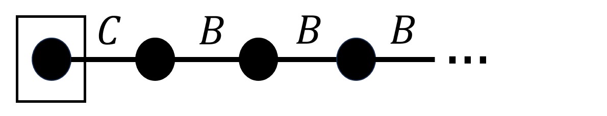
($a$)    ($b$)

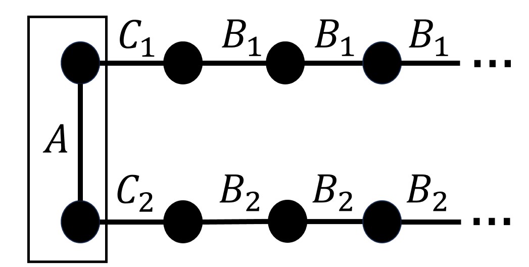
Figure 4: ($a$) Single-site bath model. ($b$) Two-site bath model considered in the main article.

Now consider our main example with $C_{1}=C$, $C_{2}=3C$, $B_{1}=B$, $B_{2}=2B$. Since $A$ could be zero, we expect the single site conditions $C\leq\sqrt{2}B$ and $(3C)\leq\sqrt{2}(2B)$ to be required for decay. In general, the condition for decay will be more complicated in the coupled system.

The product $S_{1}(z)S_{2}(z)$ is complex in the region $|z|<4B$. Due to these imaginary parts, there cannot be poles in this region. Now consider $4B<|z|$. In this region $S_{1}(z)$ an $S_{2}(z)$ are monotonic increasing functions. Thus if $S_{1}(z)S_{2}(z)>|A|^{2}$ at $z=4B$, then there will be no zeros in any region. To determine the parameter bounds we check when $S_{1}(z)S_{2}(z)=|A|^{2}$ for $z=4B$. This condition is

$$(4B-\frac{2C^{2}}{4B+\sqrt{2B}\sqrt{6B}})(4B-\frac{18C^{2}}{4B})=|A|^{2}.$$ (26)

Define $b_{A}=B/A$, $c_{A}=C/A$, $x_{0}=1/(2+\sqrt{3})$ and $y_{0}=9/2$. Then we can rewrite eq. (26) as

$$c_{A}^{2}=\frac{2b_{A}^{2}(x_{0}+y_{0})\pm\sqrt{4b_{A}^{4}(x_{0}-y_{0})^{2}+x_{0}y_{0}b_{A}^{2}}}{x_{0}y_{0}}$$ (27)

Considering the decay requirement $S_{1}S_{2}>|A|^{2}$, we have the condition for no zeros in the denominator as

$$c_{A}^{2}<\frac{2b_{A}^{2}(x_{0}+y_{0})-\sqrt{4b_{A}^{4}(x_{0}-y_{0})^{2}+x_{0}y_{0}B_{A}^{2}}}{x_{0}y_{0}}.$$ (28)

This defines the blue curve plotted in 2. This condition implies a number of other inequalities

$$C<\sqrt{2}B\ ,\ (3C)<\sqrt{2}(2B)\ ,\ 9\gamma<8B\ ,\ A<4B.$$ (29)

Appendix D Numerical Methods

Consider the Green’s functions $\bar{G}_{r,s}(z)$ defined in eqs. (C) and (23). In the singular and weak coupling limits, these Green’s functions match up with $G_{r,s}(z)$ defined in eq. (C). However, even outside of the two limits, the function $\bar{G}_{r,s}(z)$ can be used to help the numerics converge better.

The $\bar{G}_{r,s}(z)$ functions have known Fourier transforms when plugged into eq. (13). That is, we have

$$\bar{g}_{1,1}(t) = \frac{-\text{i}}{Z_{+}-Z_{-}}\left(e^{-\text{i}Z_{+}t}(Z_{+}+\text{i}\frac{C_{2}^{2}}{B_{2}})-e^{-\text{i}Z_{-}t}(Z_{-}+\text{i}\frac{C_{2}^{2}}{B_{2}})\right)$$

$$\bar{g}_{1,2}(t) = \frac{-\text{i}A}{Z_{+}-Z_{-}}\left(e^{-\text{i}Z_{+}t}-e^{-\text{i}Z_{-}t}\right)$$

$$\bar{g}_{2,1}(t) = \frac{-\text{i}A^{*}}{Z_{+}-Z_{-}}\left(e^{-\text{i}Z_{+}t}-e^{-\text{i}Z_{-}t}\right)$$

$$\bar{g}_{2,2}(t) = \frac{-\text{i}}{Z_{+}-Z_{-}}\left(e^{-\text{i}Z_{+}t}(Z_{+}+\text{i}\frac{C_{1}^{2}}{B_{1}})-e^{-\text{i}Z_{-}t}(Z_{-}+\text{i}\frac{C_{1}^{2}}{B_{1}})\right)$$

with

$$Z_{\pm}=\frac{-\text{i}(\gamma_{1}+\gamma_{2})\pm\sqrt{4|A|^{2}-(\gamma_{1}-\gamma_{2})^{2}}}{2}.$$

There are numerical challenges if $Z_{+}=Z_{-}$. However, we have checked numerically that Fig. 2 of the main article does not have this exact condition for any of the discretely evaluated grid points.

Now we numerically take the Fourier transform from eq. (12) of

$$\Delta G_{r,s}(z)=G_{r,s}(z)-\bar{G}_{r,s}(z)$$ (32)

with the limits of the energy integration as $-D$ to $D$ with $D=800$. We call the Fourier transform of $\Delta G_{r,s}(z)$ as $\Delta g_{r,s}(t)$. Then we take in our analysis the Green’s functions

$$g_{r,s}(t)=\bar{g}_{r,s}(t)+\Delta g_{r,s}(t)$$ (33)

That is, the $g_{r,s}(t)$ we use in the main text is the sum of the analytical $\bar{g}_{r,s}(t)$ of eq. (LABEL:timeGreenBar) plus the numerically calculated $\Delta g_{r,s}(t)$. The process defined above is numerically well behaved.

References

- Breuer and Petruccione [2002] H. P. Breuer and F. Petruccione, The Theory of Open Quantum Systems (Oxford University Press, New York, 2002).
- Raimond and Haroche [2006] J.-M. Raimond and S. Haroche, Exploring the quantum, Vol. 82 (2006) p. 86.
- Naghiloo et al. [2019] M. Naghiloo, M. Abbasi, Y. N. Joglekar, and K. Murch, Quantum state tomography across the exceptional point in a single dissipative qubit, Nature Physics 15, 1232 (2019).
- Abbasi et al. [2022] M. Abbasi, W. Chen, M. Naghiloo, Y. N. Joglekar, and K. W. Murch, Topological quantum state control through exceptional-point proximity, Phys. Rev. Lett. 128, 160401 (2022).
- Lin et al. [2013] Y. Lin, J. Gaebler, F. Reiter, T. R. Tan, R. Bowler, A. Sørensen, D. Leibfried, and D. J. Wineland, Dissipative production of a maximally entangled steady state of two quantum bits, Nature 504, 415 (2013).
- Ding et al. [2021] L. Ding, K. Shi, Q. Zhang, D. Shen, X. Zhang, and W. Zhang, Experimental determination of -symmetric exceptional points in a single trapped ion, Phys. Rev. Lett. 126, 083604 (2021).
- Kamakari et al. [2022] H. Kamakari, S.-N. Sun, M. Motta, and A. J. Minnich, Digital quantum simulation of open quantum systems using quantum imaginary–time evolution, PRX Quantum 3, 010320 (2022).
- Lindblad [1976] G. Lindblad, On the generators of quantum dynamical semigroups, Communications in mathematical physics 48, 119 (1976).
- Gorini et al. [1976] V. Gorini, A. Kossakowski, and E. C. G. Sudarshan, Completely positive dynamical semigroups of n-level systems, Journal of Mathematical Physics 17, 821 (1976).
- Manzano [2020] D. Manzano, A short introduction to the lindblad master equation, Aip advances 10 (2020).
- Palmer [1977] P. Palmer, The singular coupling and weak coupling limits, Journal of Mathematical Physics 18, 527 (1977).
- Okuma et al. [2020] N. Okuma, K. Kawabata, K. Shiozaki, and M. Sato, Topological origin of non-hermitian skin effects, Phys. Rev. Lett. 124, 086801 (2020).
- Herviou et al. [2019] L. Herviou, J. H. Bardarson, and N. Regnault, Defining a bulk-edge correspondence for non-hermitian hamiltonians via singular-value decomposition, Phys. Rev. A 99, 052118 (2019).
- Brunelli et al. [2023] M. Brunelli, C. C. Wanjura, and A. Nunnenkamp, Restoration of the non-hermitian bulk-boundary correspondence via topological amplification, SciPost Physics 15, 173 (2023).
- Porras and Fernández-Lorenzo [2019] D. Porras and S. Fernández-Lorenzo, Topological amplification in photonic lattices, Phys. Rev. Lett. 122, 143901 (2019).
- Ramos et al. [2021] T. Ramos, J. J. García-Ripoll, and D. Porras, Topological input-output theory for directional amplification, Phys. Rev. A 103, 033513 (2021).
- Monkman and Sirker [2024] K. Monkman and J. Sirker, Hidden zero modes and topology of multiband non-hermitian systems, arXiv preprint arXiv:2405.09728 (2024).
- Minganti et al. [2019] F. Minganti, A. Miranowicz, R. W. Chhajlany, and F. Nori, Quantum exceptional points of non-hermitian hamiltonians and liouvillians: The effects of quantum jumps, Phys. Rev. A 100, 062131 (2019).
- Roccati et al. [2022] F. Roccati, G. M. Palma, F. Ciccarello, and F. Bagarello, Non-hermitian physics and master equations, Open Systems & Information Dynamics 29, 2250004 (2022).
- Bergholtz et al. [2021] E. J. Bergholtz, J. C. Budich, and F. K. Kunst, Exceptional topology of non-hermitian systems, Rev. Mod. Phys. 93, 015005 (2021).
- Hatano [2019] N. Hatano, Exceptional points of the lindblad operator of a two-level system, Molecular Physics 117, 2121 (2019).
- Zhu [2018] Z. Zhu, Excitonic modes and phonons in biological molecules, Ph.D. thesis, University of British Columbia (2018).
- Mitchison and Plenio [2018] M. T. Mitchison and M. B. Plenio, Non-additive dissipation in open quantum networks out of equilibrium, New Journal of Physics 20, 033005 (2018).