Block subspace expansions for eigenvalues and eigenvectors approximation

Abstract

Let $A\in\mathbb{C}^{n\times n}$ and let $\mathcal{X}\subset\mathbb{C}^{n}$ be an $A$-invariant subspace with $\dim\mathcal{X}=d\geq 1$, corresponding to exterior eigenvalues of $A$. Given an initial subspace ${\cal V}\subset\mathbb{C}^{n}$ with $\dim{\cal V}=r\geq d$, we search for expansions of ${\cal V}$ of the form ${\cal V}+A({\cal W}_{0})$, where ${\cal W}_{0}\subset{\cal V}$ is such that $\dim{\cal W}_{0}\leq d$ and such that the expanded subspace is closer to $\mathcal{X}$ than the initial ${\cal V}$. We show that there exist (theoretical) optimal choices of such ${\cal W}_{0}$, in the sense that $\theta_{i}(\mathcal{X},{\cal V}+A({\cal W}_{0}))\leq\theta_{i}({\cal V}+A({\cal W}))$ for every ${\cal W}\subset{\cal V}$ with $\dim{\cal W}\leq d$, where $\theta_{i}(\mathcal{X},{\cal T})$ denotes the $i$-th principal angle between $\mathcal{X}$ and ${\cal T}$, for $1\leq i\leq d\leq\dim{\cal T}$. We relate these optimal expansions to block Krylov subspaces generated by $A$ and ${\cal V}$. We also show that the corresponding iterative sequence of subspaces constructed in this way approximate $\mathcal{X}$ arbitrarily well, when $A$ is Hermitian and $\mathcal{X}$ is simple. We further introduce computable versions of this construction and compute several numerical examples that show the performance of the computable algorithms and test our convergence analysis.

MSC(2000) subject classification: 65F15, 15A18, 65F10.

Keywords: optimal subspace expansion, eigenvector approximation, block Krylov subspace, projection methods, computable subspace expansion.

1 Introduction

The approximation of eigenvalues and eigenvectors of a large complex matrix $A\in\mathbb{C}^{n\times n}$ is a central topic in numerical linear algebra. Given an initial search subspace ${\cal V}_{0}\subset\mathbb{C}^{n}$, there are several projection methods that allow to compute approximations of the eigenvalues and eigenvectors of $A$ based on ${\cal V}_{0}$. This has motivated the development of different techniques to expand the search subspace ${\cal V}_{0}\subset{\cal V}_{1}(A,{\cal V}_{0})$ in such a way that the enlarged subspace provides better approximations of eigenvalues and eigenvectors of $A$ than the initial ${\cal V}_{0}$. One popular expansion method is the block Krylov subspace method (for a detailed account on these methods see [19, 23, 24]). In this work we consider (optimal) expansions of the search subspace based on augmentation/deflation techniques that extend the recent results in [10] for the approximation eigenvalues and eigenvectors to the case of simultaneous approximation of the exterior $d$ eigenvalues and eigenvectors of $A$ as follows.

Consider a $d$-dimensional subspace $\mathcal{X}\subset\mathbb{C}^{n}$ that is invariant for $A\in\mathbb{C}^{n\times n}$. In this case the eigenvalues $\lambda_{1},\ldots,\lambda_{d}$ of the restriction of $A$ to $\mathcal{X}$ are (some of the) eigenvalues of $A$; we further assume that these are exterior eigenvalues. For example, if $A$ is Hermitian we can be interested in computing the smallest eigenvalues of $A$ and their corresponding eigenvectors. On the other hand, if $A=(B^{*}B)^{1/2}$ is the operator modulus of an arbitrary matrix $B\in\mathbb{C}^{m\times n}$ then we can be interested in computing the largest eigenvalues of $A$ and their corresponding eigenvectors, that are the largest singular values and their corresponding right-singular vectors of $B$ (that generate the so-called dominant subspaces of $B$). In these situations, the information contained in $(\mathcal{X},\{\lambda_{i}\}_{i=1}^{d})$ can be used to approximate the action of $A$ as a linear operator (for example, if $A=(B^{*}B)^{1/2}$ then we can use $(\mathcal{X},\{\lambda_{i}\}_{i=1}^{d})$ to construct optimal low rank approximations of $B$). When $A$ is a large matrix the direct computation of $(\mathcal{X},\{\lambda_{i}\}_{i=1}^{d})$ can require too much time, or memory space, or it could simply be impractical. Thus, one of the major tasks in numerical linear algebra is to compute efficient and fast approximations of this data.

In this setting we are interested in computing approximations of $\mathcal{X}$ in terms of iterative algorithms of the following type: given a subspace ${\cal V}\subset\mathbb{C}^{n}$ such that $d:=\dim\mathcal{X}\leq r:=\dim{\cal V}$, the algorithm expands (in each step) the search space ${\cal V}$ by considering ${\cal V}+A({\cal W}_{0})$, for some subspace ${\cal W}_{0}\subset{\cal V}$ with $\dim{\cal W}_{0}=d$. We are interested in optimal choices of the expanded subspaces ${\cal V}+A({\cal W}_{0})$ (in each step). Hence, we further impose that ${\cal V}+A({\cal W}_{0})$ lies the closest to $\mathcal{X}$ among subspaces of the form ${\cal V}+A({\cal W})$, for ${\cal W}\subset{\cal V}$ with $\dim{\cal W}=d$. As a (vector valued) measure of distance between subspaces we consider the so-called principal angles. Thus, we search for ${\cal W}_{0}\subset{\cal V}$ with $\dim{\cal W}_{0}=d$ and such that

$$\Theta(\mathcal{X}\,,\,{\cal V}+A({\cal W}_{0}))\leq\Theta(\mathcal{X}\,,\,{\cal V}+A({\cal W}))$$ (1)

for every subspace ${\cal W}\subset{\cal V}$ with $\dim{\cal W}=d$. Here $\Theta(\mathcal{X},\mathcal{Y})$ denotes the diagonal matrix with diagonal entries given by the principal angles between $\mathcal{X}$ and $\mathcal{Y}$, denoted $0\leq\theta_{1}(\mathcal{X},\mathcal{Y})\leq\ldots\leq\theta_{k}(\mathcal{X},\mathcal{Y})\leq\pi/2$, where $k=\min\{\dim\mathcal{X},\dim\mathcal{Y}\}$. In case $d=1$ i.e., $\mathcal{X}=\text{span}\{x_{1}\}$, this problem was originally considered by Ye [27]. Recently, Jia [10] has extended the results in [27] and obtained several fundamental insights related with computable iterative algorithms that provide approximations of the optimal subspace expansion ${\cal V}+A(\text{span}\{w_{0}\})$. As mentioned in [10, 27] even in this particular setting, the choice of $w\in{\cal V}$ has a relevant impact on the proximity between ${\cal V}+\text{span}\{A(w)\}$ and the target subspace $\mathcal{X}$, when the initial subspace ${\cal V}$ lacks of structure (which is the typical case for initial subspaces ${\cal V}$ induced by random matrices).

In this work we show that there exist subspaces ${\cal W}_{0}$ as in Eq. (1). Our approach differs from those in [10, 27]. Indeed, we replace the optimization arguments from those works (involved in the computation of principal angles) with a rather simple optimization problem: namely, for subspaces ${\cal S},\,\mathcal{X}\subset\mathbb{C}^{n}$ with $\dim{\cal S}\geq\dim\mathcal{X}=d$ our approach is based on the computation of those subspaces ${\cal T}\subset{\cal S}$ such that $\dim{\cal T}=d$ and $\Theta(\mathcal{X},{\cal S})=\Theta(\mathcal{X},{\cal T})$. As for the case $d=1$ (see [10, 27]), the construction of such ${\cal W}_{0}$ involves the target subspace $\mathcal{X}$. Thus, although the expansions ${\cal V}+A({\cal W}_{0})$ are optimal, they are not computable and hence have no use for the numerical approximation of $\mathcal{X}$. Nevertheless, the theoretical iterative algorithm derived from the optimal (block) subspace expansions ${\cal V}+A({\cal W}_{0})$ serves as a reference for the assessment of the numerical performance of computable iterative algorithms that in each step expand the initial subspace ${\cal V}$ by considering ${\cal V}+A(\tilde{\cal W})$, for some computable $\tilde{\cal W}\subset{\cal V}$ with $\dim\tilde{\cal W}\leq d$. As a first step towards the analysis of this general theoretical algorithm, we consider an Hermitian matrix $A\in\mathbb{C}^{n\times n}$ and obtain a proximity analysis of the (finite) sequence $({\cal V}_{t})_{t=0}^{q}$ of subspaces such that

$${\cal V}_{0}={\cal V}\,,\ {\cal V}_{t}={\cal V}_{t-1}\oplus{\cal N}_{t}\subset{\cal V}_{t-1}+A({\cal V}_{t-1})\quad\text{ and }\quad\dim{\cal N}_{t}\leq d$$

in such a way that ${\cal N}_{t}$ has an explicit formula in terms of $A$, ${\cal V}_{t-1}$ and $\mathcal{X}$, and

$$\Theta(\mathcal{X},{\cal V}_{t})=\Theta(\mathcal{X},{\cal V}_{t-1}+A({\cal V}_{t-1}))\,,\ \ t\in\mathbb{I}_{q}\,$$

where $\mathbb{I}_{q}=\{1,\ldots,q\}$. We remark that ${\cal V}_{t}={\cal V}_{t-1}+A({\cal W}_{t})$, for some ${\cal W}_{t}\subset{\cal V}_{t-1}$ with $\dim{\cal W}_{t}\leq d$, for $t\in\mathbb{I}_{q}$ (with the notation of the first part of this paragraph, we relax the condition $\dim{\cal W}_{0}=d$ and consider optimal expansions with $\dim{\cal W}_{0}\leq d$). In this context we show that if $\|\cdot\|$ is an arbitrary unitarily invariant norm then $\|\tan(\Theta(\mathcal{X},{\cal V}_{t}))\|$ decays as $((\lambda_{d+1}-\lambda_{n})/(\lambda_{d}-\lambda_{n}))^{t}$, where $\lambda_{1}\geq\ldots\geq\lambda_{n}$ denote the eigenvalues of $A$ counting multiplicities and arranged in non-increasing order. Our novel perspective on the optimal (block) subspace expansion problem allow us to show that the (computable) block Krylov sequence of subspaces

$$\mathcal{K}_{0}={\cal V}\,,\ \mathcal{K}_{t}=\mathcal{K}_{t-1}+A(\mathcal{K}_{t-1})\quad\text{ for }\quad t\in\mathbb{I}_{q}\ ,$$

is a natural frame (and a source for comparison) for the (theoretical) sequence $\{{\cal V}_{t}\}_{t=0}^{q}$.

Once the proximity analysis of the optimal (block) subspace expansion algorithm is obtained in the Hermitian case, similar to [10] we develop some computable versions of the algorithm based on the Rayleigh-Ritz or the refined Rayleigh-Ritz (projection) methods [5, 6, 7, 8, 10, 13]. Thus, we consider derived computable iterative algorithms that produce finite sequences $\{\widehat{\cal V}_{t}\}_{t=0}^{q}$ with

$$\widehat{\cal V}_{0}={\cal V}\,,\ \widehat{\cal V}_{t}=\widehat{\cal V}_{t-1}\oplus\widehat{\cal N}_{t}\ ,\ \ t\in\mathbb{I}_{q}$$

such that in each step they expand the search space by $\widehat{\cal N}_{t}$, which is a computable version of the (theoretical) subspace ${\cal N}_{t}$ considered above. Since our theoretical approach to the optimal expansion problem differs from previous works, so do our derived numerical algorithms. We include implementations of these computable algorithms, together with some numerical examples that allow us to compare the different algorithms: block Krylov method, optimal (theoretical) expansions and computable expansions of the search spaces for the approximation of invariant subspaces associated with exterior (largest) eigenvalues of Hermitian matrices. Even when ${\cal V}_{t}\subset\mathcal{K}_{t}$, $\dim\mathcal{K}_{t}=(r+1)\cdot t$ and $\dim{\cal V}_{t}=r+d\cdot t$ (in the generic case), for $t\in\mathbb{I}_{q}$, the examples show that in some cases the subspaces ${\cal V}_{t}$ (and their computable counterparts) provide approximations of $\mathcal{X}$ that are comparable with those obtained from $\mathcal{K}_{t}$. In these cases, the ${\cal V}_{t}$’s provide good approximations of $\mathcal{X}$ through subspaces of much lower dimension than the dimensions of the corresponding $\mathcal{K}_{t}$’s. On the other hand, there are numerical examples in which the block Krylov method outperforms the theoretical approximations provided by the ${\cal V}_{t}$’s and (their computable counterparts).

Our work can be framed into the design and analysis of (block) iterative search subspace expansion algorithms for the simultaneous approximation of eigenvalues and eigenvectors of large matrices. Notice that the expansion is obtained in terms of an augmentation-deflation technique namely ${\cal V}\mapsto{\cal V}+A({\cal V})\mapsto{\cal V}+A({\cal W}_{0})$ where ${\cal V}+A({\cal W}_{0})\subset{\cal V}+A({\cal V})$, or ${\cal V}\mapsto{\cal V}+A({\cal V})\mapsto{\cal V}\oplus{\cal N}$ where ${\cal V}\oplus{\cal N}\subset{\cal V}+A({\cal V})$. Hence, our work can be considered within (one-step) restarted block Krylov algorithms for the approximation of eigenvectors and eigenvalues of large matrices. There are several works that deal with similar problems. As we have already mentioned, in [10, 27] Ye and Jia considered the optimal (theoretical) expansion algorithms together with some of their computable versions, in which in each step the search space increases its dimension by one. In [15] (see also [14]) Lee and Stewart considered a block expansion of the search subspace in terms of residual vectors corresponding to the Rayleigh-Ritz method. In [26], this approach was modified by considering residual vectors corresponding to the refined Rayleigh-Ritz method, introduced by Jia in [6]. Another popular iterative method for the approximation of interior eigenvalues and eigenvectors based on the expansion of the search subspace is the Jacobi-Davidson method, introduced in [21, 22] (see also [4]). All these methods are constructed in such a way that the expanded search space provides better approximations of eigenvalues and eigenvectors of matrices. Most of these methods can be implemented using specific (mathematical) software. While our approach is based on a theoretical (i.e. not computable) algorithm, we show that its numerical computable versions (induced by simple projection methods) also provide good numerical approximations with the advantage of controlling the size of the stored information in each step (through the control of the dimension of the expanded search space). Furthermore, our computable approach can be extended to deal with the approximation of interior eigenvalues and eigenvectors, by applying different projections methods (i.e. harmonic Rayleigh-Ritz, refined harmonic Rayleigh-Ritz and shift-invert methods, see [9, 11, 12]).

The paper is organized as follows. We include some brief preliminaries in Section 2. In Section 3 we present our main results and delay their proofs until Section 4. In more detail, in Section 3.1 we obtain a complete solution of the optimal subspace expansion problem. We further propose a variation of the optimal expansion problem and describe an explicit algorithmic construction of solutions to this problem (in terms of closed formulas involving the target subspace). We show that the proposed algorithm constructs a sequence of increasing subspaces that are related to some block Krylov subspaces. In Section 3.2 we obtain a proximity analysis of the algorithmic construction of the optimal subspace expansions together with a proximity analysis of associated block Krylov subspaces in the Hermitian case. In Section 3.3 we follow recent ideas of Jia [10] and consider algorithms that construct computable expansions of subspaces based on projection methods. In Section 4 we present the proofs of our main results, based on some technical results. We defer the proof of these technical results to Section 6. Finally, in Section 5 we include the analysis of several numerical examples obtained by implementation the Algorithms considered in Sections 3.2 and 3.3.

2 Preliminaries

Notation and terminology. We let $\mathbb{C}^{m\times n}$ be the space of complex $m\times n$ matrices with entries in $\mathbb{C}$. A norm $\|\cdot\|$ in $\mathbb{C}^{n\times n}$ is unitarily invariant (briefly u.i.n.) if $\|UAV\|=\|A\|$, for every $A\in\mathbb{C}^{n\times n}$ and unitary matrices $U,\,V\in\mathbb{C}^{n\times n}$. For example, the operator and Frobenius norms, denoted by $\|\cdot\|_{2}$ and $\|\cdot\|_{F}$ respectively, are u.i.n.’s. If ${\cal V}\subset\mathbb{C}^{n}$ is a subspace, we let $P_{\cal V}\in\mathbb{C}^{n\times n}$ denote the orthogonal projection onto ${\cal V}$.

For $A\in\mathbb{C}^{m\times n}$ we will denote it’s Moore–Penrose pseudo-inverse as $A^{\dagger}$ . Among other basic properties of the pseudo-inverse we will use the fact that $AA^{\dagger}=P_{R(A)}$ and $A^{\dagger}A=P_{\ker(A)^{\perp}}=P_{R(A^{*})}$ where $R(A)$ denotes the subspace of $\mathbb{C}^{m}$ spanned by the columns of $A$.

For $n\in\mathbb{N}$, let $\mathbb{I}_{n}=\{1,\ldots,n\}$. Given a vector $x\in\mathbb{C}^{n}$ we denote by $\text{diag}(x)\in\mathbb{C}^{n\times n}$ the diagonal matrix whose main diagonal is $x$. If $x=(x_{i})_{i\in\mathbb{I}_{n}}\in\mathbb{R}^{n}$ we denote by $x^{\downarrow}=(x_{i}^{\downarrow})_{i\in\mathbb{I}_{n}}$ the vector obtained by rearranging the entries of $x$ in non-increasing order. We also use the notation $(\mathbb{R}^{n})^{\downarrow}=\{x\in\mathbb{R}^{n}\ :\ x=x^{\downarrow}\}$ and $(\mathbb{R}_{\geq 0}^{n})^{\downarrow}=\{x\in\mathbb{R}_{\geq 0}^{n}\ :\ x=x^{\downarrow}\}$.

Given an Hermitian matrix $A\in\mathbb{C}^{n\times n}$ we denote by $\lambda(A)=(\lambda_{i}(A))_{i\in\mathbb{I}_{n}}\in(\mathbb{R}^{n})^{\downarrow}$ the eigenvalues of $A$ counting multiplicities and arranged in non-increasing order. For $B\in\mathbb{C}^{m\times n}$ we let $s(B)=\lambda(|B|)\in(\mathbb{R}_{\geq 0}^{n})^{\downarrow}$ denote the singular values of $B$, i.e. the eigenvalues of the positive semi-definite matrix $|B|=(B^{*}B)^{1/2}\in\mathbb{C}^{n\times n}$.

Principal angles between subspaces. Let ${\cal S},\,\mathcal{X}\subset\mathbb{C}^{n}$ be subspaces such that $d=\dim\mathcal{X}\leq\dim{\cal S}$. Recall that the principal angles between $\mathcal{X}$ and ${\cal S}$, denoted $\theta_{1},\ldots,\theta_{d}\in[0,\pi/2]$ are given by

$$\cos(\theta_{i})=s_{i}(P_{\cal S}P_{\mathcal{X}})=s_{i}(P_{\mathcal{X}}P_{\cal S})\quad\text{ for }\quad 1\leq i\leq d\,.$$

Notice that by construction $0\leq\theta_{1}\leq\ldots\leq\theta_{d}\leq\pi/2$. We let

$$\Theta(\mathcal{X},\,{\cal S})=\text{diag}(\theta_{1},\ldots,\theta_{d})\,.$$

Principal angles allow to define metrics between subspaces [16], which are use in a wide range of applications (see [16, Section 1] and the references therein). In order to save notation, whenever we have matrices $X$ and $V$ with the same number of rows we will write $\Theta(X,V)$ instead of $\Theta(R(X),R(V))$. $\triangle$

3 Main results

In this section we present our main results. In Section 3.1 we solve the optimal (block) subspace expansion problem (for details see below) and find an alternative (relaxed) formulation for an optimal expanded search space. This alternative formulation induces an iterative process that we describe in terms of a pseudo-code in Algorithm 3.1. We compare the sequence of subspaces that are the outputs of Algorithm 3.1 with the sequence of block Krylov spaces, where both sequences are induced by a matrix $A\in\mathbb{C}^{n\times n}$ and an initial subspace ${\cal V}\subset\mathbb{C}^{n}$. In Section 3.2 we obtain a proximity analysis of the output of Algorithm 3.1 and of the sequence of block Krylov spaces, to the eigenspaces of a Hermitian matrix $A$ associated to its exterior (largest) eigenvalues. In Section 3.3 we follow ideas from [10] and describe pseudo-codes in Algorithm 3.2 for the iterative construction of computable (sub)optimal (block) subspace expansions. In Section 5 we include several numerical examples related to the algorithms considered in Sections 3.2 and 3.3.

3.1 Optimal (block) subspace expansion problem

Our first results are related to the optimal (block) subspace expansion problem. Hence, we fix a $d$-dimensional subspace $\mathcal{X}\subset\mathbb{C}^{n}$ that is invariant for $A\in\mathbb{C}^{n\times n}$. We consider an initial (guess) subspace ${\cal V}\subset\mathbb{C}^{n}$ such that $r=\dim{\cal V}\geq d$. In this setting, we search for the optimal subspaces ${\cal W}_{0}\subset{\cal V}$ with $\dim{\cal W}_{0}=d$ and such that

$$\Theta(\mathcal{X}\,,\,{\cal V}+A({\cal W}_{0}))\leq\Theta(\mathcal{X}\,,\,{\cal V}+A({\cal W}))$$ (2)

for every subspace ${\cal W}\subset{\cal V}$ with $\dim{\cal W}=d$. If ${\cal W}\subset{\cal V}$ with $\dim{\cal W}=d$, let $\mathcal{E}={\cal V}+A({\cal W})$ and notice that

$$\mathcal{E}\subset{\cal S}:={\cal V}+A({\cal V})\quad\text{ is such that }\quad{\cal V}\subset\mathcal{E}\quad\text{ and }\quad\dim\mathcal{E}\leq r+d\,.$$

Thus, as a first step towards the solution of (2), we can consider the following relaxation of the problem in Eq. (2): find $\mathcal{E}_{0}\subset{\cal S}$ such that ${\cal V}\subset\mathcal{E}_{0}$, $\dim\mathcal{E}_{0}\leq r+d$ and such that

$$\Theta(\mathcal{X}\,,\,\mathcal{E}_{0})\leq\Theta(\mathcal{X}\,,\,\mathcal{E})$$ (3)

for every such $\mathcal{E}$ as above. The advantage of considering the problem in Eq. (3) is that its solution can be described in simple terms: indeed, if we let ${\cal M}=P_{\cal S}(\mathcal{X})\subset{\cal S}$ then, every ${\cal V}+{\cal M}\subset\mathcal{E}_{0}\subset{\cal S}$ with $\dim\mathcal{E}_{0}\leq r+d$ satisfies Eq. (3). Furthermore, using the fundamental identity

$${\cal S}={\cal V}+A({\cal V})={\cal V}\oplus(1-P_{\cal V})A({\cal V})$$ (4)

we can easily construct $\mathcal{E}_{0}$ as above such that $\mathcal{E}_{0}={\cal V}+A({\cal W}_{0})$, for some ${\cal W}_{0}\subset{\cal V}$ with $\dim{\cal W}_{0}=d$ (for the proofs of both of these assertions, see Section 4). Notice that, since $\mathcal{E}_{0}$ is a solution to the relaxed problem, such ${\cal W}_{0}$ satisfies Eq. (2) and hence, it is a solution to the original optimal subspace expansion problem. To describe the main result of this section we include the following:

Notation 3.1.

In what follows we consider:

1. $A\in\mathbb{C}^{n\times n}$ and an $A$-invariant subspace $\mathcal{X}\subseteq\mathbb{C}^{n}$, with $\dim\mathcal{X}=d$.

2. A subspace ${\cal V}\subset\mathbb{C}^{n}$ with $\dim{\cal V}:=r\geq d$, $\mathcal{X}\not\subseteq{\cal V}$ and $A({\cal V})\not\subseteq{\cal V}$.

3. Let $V\in\mathbb{C}^{n\times r}$ have orthonormal columns such that $R(V)={\cal V}$ and set

   $$R:=AV-V(V^{*}AV)=(1-P_{\cal V})AV\in\mathbb{C}^{n\times r}\,.$$

   $\triangle$

Theorem 3.2.

Consider Notation 3.1. Denote by ${\cal S}:={\cal V}+A({\cal V})$. Then,

1. There exist subspaces ${\cal W}_{0}\subseteq{\cal V}$ with $\dim{\cal W}_{0}=d$ such that

   $$\Theta(\mathcal{X}\,,\,{\cal V}+A({\cal W}_{0}))=\Theta(\mathcal{X}\,,\,{\cal S})=\min\{\Theta(\mathcal{X}\,,\,{\cal V}+A({\cal W})):{\cal W}\subseteq{\cal V}\,,\,\dim{\cal W}=d\}\ .$$ (5)

If we let ${\cal N}:=(1-P_{\cal V})(P_{\cal S}(\mathcal{X})\,)$ and $\mathcal{C}_{\rm op}=R^{\dagger}(\,{\cal N}\,)\subseteq\ker R^{\perp}\subseteq\mathbb{C}^{r}\,$ then

1. $\mathcal{C}_{\rm op}=R^{\dagger}\mathcal{X}$ , ${\cal N}=RR^{\dagger}\mathcal{X}=R(\mathcal{C}_{\rm op})$, and ${\cal S}={\cal V}\oplus R(\mathbb{C}^{r})$.

2. The subspaces ${\cal W}_{0}$ which satisfy Eq. (5) are exactly those of the form

   $${\cal W}_{0}=V(\mathcal{C}_{0})\quad\text{ for some \ \ $\mathcal{C}_{0}\subseteq\mathbb{C}^{r}$ \ \ with \ \ $\dim\mathcal{C}_{0}=d$ \ \ and }\quad\mathcal{C}_{\rm op}\subseteq P_{\ker R^{\perp}}\mathcal{C}_{0}\ .$$ (6)

   In particular, ${\cal V}\oplus{\cal N}={\cal V}\oplus R(\mathcal{C}_{\rm op})\subset{\cal V}\oplus R(\mathcal{C}_{0})={\cal V}\oplus(1-P_{\cal V})A({\cal W}_{0})={\cal V}+A({\cal W}_{0})$.

3. If ${\cal V}\cap A^{-1}({\cal V})=\{0\}$ and $\dim{\cal N}=d$, then ${\cal W}_{0}$ as in Eq. (5) is unique and given by

   $${\cal W}_{0}=V(\mathcal{C}_{\rm op})=V\,R^{\dagger}(\mathcal{X})\quad\text{ with }\quad{\cal V}+A({\cal W}_{0})={\cal V}\oplus{\cal N}\,.$$

Proof.

See Section 4. $\square$

Remark 3.3.

We show how to deduce [10, Theorem 2.2] from our previous result. Indeed, consider the notation from Theorem 3.2 and assume that $d=1$. Hence, $\mathcal{X}=\mathbb{C}\cdot x$, for some $x\in\mathbb{C}^{n}$ such that $Ax=\lambda\,x$. Assume further (as in [10, Theorem 2.2]) that $x\notin{\cal V}$, ${\cal V}\cap A^{-1}({\cal V})=\{0\}$ and that $RR^{\dagger}x\neq 0$ (i.e. $\dim{\cal N}=1=d$).

By item 4. in Theorem 3.2 we get that the unique optimal subspace ${\cal W}_{0}$ is spanned by $w_{0}=VR^{\dagger}x$ and that ${\cal V}_{\rm op}:={\cal V}+\mathbb{C}\cdot A(w_{0})={\cal V}\oplus\mathbb{C}\cdot RR^{\dagger}x$. This last fact implies that $(1-P_{\cal V})A(w_{0})\in\mathbb{C}\cdot RR^{\dagger}x$. By items 1. and 2. in Theorem 3.2 we get that

$$\angle({\cal V}_{\rm op},x)=\angle({\cal S},x)=\angle(P_{{\cal S}}x,x)=\angle(P_{{\cal V}}x+RR^{\dagger}x,x)$$

Moreover, our approach shows that the auxiliary subspace ${\cal V}_{R}={\cal V}\oplus R(\mathbb{C}^{r})$ considered in [10] coincides with ${\cal V}_{R}={\cal S}\,(={\cal V}+A({\cal V}))$ (see item 2. in Theorem 3.2). Indeed, we have exploited this last fact by introducing (in the general case $d\geq 1$) a natural comparison between the subspaces ${\cal V}_{\rm op}$ and the block Krylov subspaces ${\cal S}={\cal V}+A({\cal V})$ throughout our work (see Remark 3.5 below). $\triangle$

Consider the notation from Theorem 3.2. As pointed out by Jia in [10] in case $d=1$, it is convenient to focus on the optimal expanded space ${\cal V}+A({\cal W}_{0})\subset\mathbb{C}^{n}$ rather than the subspace ${\cal W}_{0}\subset{\cal V}$. After all, we are interested in the optimal search space ${\cal V}+A({\cal W}_{0})$ which contains $d$-dimensional subspaces that are the closest to $\mathcal{X}$, among all such subspaces. Furthermore, if we are willing to relax the problem and consider optimal search subspaces ${\cal V}+A({\cal W}^{\prime})$ for subspaces ${\cal W}^{\prime}\subset{\cal V}$ with $\dim{\cal W}^{\prime}\leq d$ (instead of asking that $\dim{\cal W}^{\prime}=d$), then we can obtain simple procedures to compute such optimal subspaces. The following result, that describes optimal search subspaces ${\cal V}+A({\cal W}^{\prime})$ as above, will play a key role in the rest of our work.

Corollary 3.4.

Consider Notation 3.1. Let ${\cal S}={\cal V}+A({\cal V})$ and ${\cal N}=(1-P_{\cal V})(P_{\cal S}(\mathcal{X})\,)$ as in Theorem 3.2. Then,

1. ${\cal V}\oplus{\cal N}={\cal V}+P_{\cal S}(\mathcal{X})\subseteq{\cal S}$, $\dim{\cal N}\leq d$ so $\dim{\cal V}\oplus{\cal N}\leq r+d$;

2. If we let ${\cal W}^{\prime}=VR^{\dagger}({\cal N})\subset{\cal V}$ then $\dim{\cal W}^{\prime}\leq d$ and

   $${\cal N}=(1-P_{\cal V})A({\cal W}^{\prime})\implies{\cal V}\oplus{\cal N}={\cal V}+A({\cal W}^{\prime})\,.$$

3. In the general case, $\Theta(\mathcal{X}\,,\,{\cal V}\oplus{\cal N})=\Theta(\mathcal{X}\,,\,{\cal S})$. Hence,

   $$\Theta(\mathcal{X}\,,\,{\cal V}\oplus{\cal N})=\Theta(\mathcal{X}\,,\,{\cal V}+A({\cal W}^{\prime}))=\min\{\Theta(\mathcal{X}\,,\,{\cal V}+A({\cal W})):{\cal W}\subset{\cal V}\,,\,\dim{\cal W}\leq d\}\ .$$

4. If we assume further that $\dim{\cal N}=d$ then, for every ${\cal W}_{0}\subset{\cal V}$ satisfying Eq. (5) we have that

   $${\cal V}+A({\cal W}_{0})={\cal V}\oplus{\cal N}\,.$$

Proof.

See Section 4. $\square$

Notice that Corollary 3.4 provides a simple construction (with explicit formulas in terms of $A$, $\mathcal{X}$ and ${\cal V}$) of an optimal expanded search subspace ${\cal V}\oplus{\cal N}$ (compare item 1. in Theorem 3.2 with item 3. in Corollary 3.4) with the additional property that ${\cal V}$ and ${\cal N}$ are mutually orthogonal. We can iterate this construction and obtain an algorithmic procedure that constructs sequences of step-wise optimal expanded search spaces as follows.

Algorithm 3.1 Optimal theoretical (block) subspace expansion

0:  $A\in\mathbb{C}^{n\times n}$, $\mathcal{X},\,{\cal V}\subset\mathbb{C}^{n}$ as in Notation 3.1; an integer $q\geq 0$ (number of iterations).

1:  Set ${\cal V}_{0}={\cal V}$. For $1\leq t\leq q$ define recursively:

1. ${\cal S}_{t}={\cal V}_{t-1}+A({\cal V}_{t-1})$;

2. ${\cal N}_{t}=(1-P_{{\cal V}_{t-1}})P_{{\cal S}_{t}}(\mathcal{X})$;

3. ${\cal V}_{t}={\cal V}_{t-1}\oplus{\cal N}_{t}$.

2:  Return: Subspaces ${\cal V}={\cal V}_{0}\subset\ldots\subset{\cal V}_{q}\subset\mathbb{C}^{n}$, such that $\Theta(\mathcal{X},{\cal S}_{t})=\Theta(\mathcal{X},{\cal V}_{t})$, for $t\in\mathbb{I}_{q}$.

Remark 3.5 (Algorithm 3.1 vs. block Krylov subspace method).

Consider Notation 3.1 and fix $q\geq 0$. Let ${\cal V}_{0}\subset\ldots\subset{\cal V}_{q}\subset\mathbb{C}^{n}$ constructed by Algorithm 3.1. Notice that given ${\cal V}_{t-1}$ then ${\cal V}_{t}$ is the optimal subspace expansion of ${\cal V}_{t-1}$ considered in Corollary 3.4, for $1\leq t\leq q$. By construction, ${\cal V}_{0}={\cal V}$ and for $1\leq t\leq q$ we get that

$${\cal V}_{t}={\cal V}_{t-1}\oplus{\cal N}_{t}={\cal V}_{t-1}+P_{{\cal S}_{t}}(\mathcal{X})\subset{\cal V}_{t-1}+A({\cal V}_{t-1})={\cal S}_{t}\,.$$

Consider the increasing family of block Krylov subspaces $\mathcal{K}_{0}\subset\ldots\subset\mathcal{K}_{q}\subset\mathbb{C}^{n}$ constructed from $A$ and ${\cal V}$. Recall that $\mathcal{K}_{0}={\cal V}$ and for $1\leq t\leq q$,

$$\mathcal{K}_{t}=A^{t}({\cal V})+A^{t-1}({\cal V})+\cdots+A({\cal V})+{\cal V}\,.$$

Alternatively, we have that $\mathcal{K}_{t}=\mathcal{K}_{t-1}+A(\mathcal{K}_{t-1})$, for $1\leq t\leq q$. It follows that ${\cal V}_{t}\subset\mathcal{K}_{t}$, for $0\leq t\leq q$. Indeed, ${\cal V}_{0}=\mathcal{K}_{0}$ and if we assume that for some $1\leq t\leq q$ we have that ${\cal V}_{t-1}\subset\mathcal{K}_{t-1}$, then

$${\cal V}_{t}\subset{\cal V}_{t-1}+A({\cal V}_{t-1})\subset\mathcal{K}_{t-1}+A(\mathcal{K}_{t-1})=\mathcal{K}_{t}\,.$$

Moreover, by construction $\dim{\cal V}_{t}\leq r+d\cdot t$ while $\dim\mathcal{K}_{t}\leq r\cdot(t+1)$, for $0\leq t\leq q$. Hence, we can expect the subspaces ${\cal V}_{t}$ to be of a (much) lower dimension than the corresponding $\mathcal{K}_{t}$, for $t\geq 1$. We point out that in the numerical examples considered in Section 5 we observed that $\dim{\cal N}_{t}=d$ and hence $\dim{\cal V}_{t}=r+d\cdot t$, while $\dim\mathcal{K}_{t}=r\cdot(t+1)$, for $0\leq t\leq q$. In particular, in each step the Algorithm 3.1 constructed the optimal subspace expansion for $A$ and the corresponding ${\cal V}_{t}$ (see item 4 in Corollary 3.4). $\triangle$

Consider the notation in Remark 3.5. There is a fundamental difference between the finite sequences $({\cal V}_{t})_{t=0}^{q}$ and $(\mathcal{K}_{t})_{t=0}^{q}$ namely, that the latter is a computable sequence of subspaces that do not depend on the target subspace $\mathcal{X}$. On the other hand, the family $({\cal V}_{t})_{t=0}^{q}$ can not be computed unless the target (typically unknown) subspace $\mathcal{X}$ is known; hence, from the numerical point of view, $({\cal V}_{t})_{t=0}^{q}$ does not provide a computable family of approximating subspaces for $\mathcal{X}$. Nevertheless, from a theoretical point of view, it is natural to ask under which conditions the family $({\cal V}_{t})_{t=0}^{q}$ approximates $\mathcal{X}$.

Problem 3.6.

Consider Notation 3.1. Let $({\cal V}_{t})_{t=0}^{q}$ be obtained from Algorithm 3.1. Find conditions (on $A$, $\mathcal{X}$ and ${\cal V}$) under which we can obtain explicit upper bounds for the decay of the principal angles $\Theta(\mathcal{X},{\cal V}_{t})$, for $t\geq 1$. $\triangle$

Problem 3.6 in its full generality seems to be hard. Notice that even when $A$ is diagonalizable, (the spectral) representations of $A$ would involve decompositions of the identity $Q_{1}+\ldots+Q_{r}=I$ in terms of (possibly non-orthogonal) projections such that $Q_{i}Q_{j}=0$ when $i\neq j$. Analysis of these situations is typically subtle. As a first step towards a better understanding of solutions of Problem 3.6 we restrict attention to the Hermitian case $A=A^{*}$ and assume further that $\mathcal{X}=\text{span}\{x_{1},\ldots,x_{d}\}$ is the subspace spanned by the eigenvectors of $A$ corresponding to the $d$ largest eigenvalues of $A$. We focus on the largest eigenvalues of $A$ only since the smallest eigenvalues of $A$ can be thought of as the largest eigenvalues of $-A$, which is also Hermitian.

3.2 Analysis of Algorithm 3.1: exterior spectra in the Hermitian case

In this section we obtain an analysis of Algorithm 3.1 in the case that $A\in\mathbb{C}^{n\times n}$ is an Hermitian matrix and that $\mathcal{X}=\text{span}\{x_{1},\ldots,x_{d}\}$ is the subspace spanned by the eigenvectors of $A$ corresponding to the $d$ largest eigenvalues of $A$. Indeed, let $\{{\cal V}_{t}\}_{t=0}^{q}$ be constructed as in Algorithm 3.1 with an initial (guess) subspace ${\cal V}$ and let $\lambda(A)=(\lambda_{i})_{i\in\mathbb{I}_{d}}\in(\mathbb{R}^{n})^{\downarrow}$ denote the eigenvalue list of $A$. If we assume that $\lambda_{d}>\lambda_{d+1}$ (which is a generic case) then we obtain an upper bound for $\Theta(\mathcal{X},{\cal V}_{t})$ that becomes arbitrarily small for large enough $t\geq 1$.

To describe the main results of this section we include the following

Notation 3.7.

In what follows we consider:

1. An Hermitian matrix $A\in\mathbb{C}^{n\times n}$ with eigenvalues list $(\lambda_{i})_{i\in\mathbb{I}_{n}}\in(\mathbb{R}^{n})^{\downarrow}$.

2. An orthonormal basis $\{x_{i}\}_{i\in\mathbb{I}_{n}}$ such that $A\,x_{i}=\lambda_{i}\,x_{i}$, for $i\in\mathbb{I}_{n}$.

3. The invariant subspace $\mathcal{X}=\text{span}\{x_{1},\ldots,x_{d}\}\subset\mathbb{C}^{n}$ and assume that $\lambda_{d}>\lambda_{d+1}$.

4. A subspace ${\cal V}\subset\mathbb{C}^{n}$ with $\dim{\cal V}:=r\geq d$, $\mathcal{X}\not\subseteq{\cal V}$ and $A({\cal V})\not\subseteq{\cal V}$. $\triangle$

Theorem 3.8.

Consider Notation 3.7 and let $\{{\cal V}_{t}\}_{t\in\mathbb{I}_{q}}$ be constructed according to Algorithm 3.1. If $\mathcal{X}\cap{\cal V}^{\bot}=\{0\}$ then for every unitarily invariant norm $\|\cdot\|$ we have

$$\|\tan(\Theta(\mathcal{X},\,{\cal V}_{t}))\|\leq\left(\frac{\lambda_{d+1}-\lambda_{n}}{(\lambda_{d}-\lambda_{n})+(\lambda_{d}-\lambda_{d+1})}\right)^{t}\|\tan(\Theta(\mathcal{X},{\cal V}_{0}))\|\,\text{, for }t\geq 1\,.$$ (7)

Proof.

See Section 4. $\square$

Notice that the hypothesis $\mathcal{X}\cap{\cal V}^{\perp}=\mathcal{X}\cap{\cal V}_{0}^{\perp}=\{0\}$ holds in a generic case. On the other hand, this condition implies that the tangents of the principal angles $\Theta(\mathcal{X},{\cal V}_{0})$, that appear in the right-hand side of Eq. (7), are well defined.

As mentioned in Remark 3.5, the block Krylov subspaces $\mathcal{K}_{0}={\cal V}$ and $\mathcal{K}_{t}=\mathcal{K}_{t-1}+A(\mathcal{K}_{t-1})$ satisfy that ${\cal V}_{t}\subset\mathcal{K}_{t}$. Hence, our result about the proximity of the ${\cal V}_{t}$’s to $\mathcal{X}$ (together with elementary properties of principal angles) imply the proximity of the $\mathcal{K}_{t}$’s to $\mathcal{X}$. Moreover, below we obtain an upper bound for $\Theta(\mathcal{X},\mathcal{K}_{t})$ that improves the upper bound derived from that for $\Theta(\mathcal{X},{\cal V}_{t})$ above. In particular, our upper bound for $\Theta(\mathcal{X},\mathcal{K}_{t})$ takes into account the so-called oversampling $\rho=r-d$, where $r=\dim{\cal V}$ denotes the dimension of the initial subspace ${\cal V}$.

Theorem 3.9.

Consider Notation 3.7 and assume that $\text{span}\{x_{1},\ldots,x_{r}\}\cap{\cal V}^{\perp}=\{0\}$. Let $\{\mathcal{K}_{t}\}_{t=0}^{q}$ be the block Krylov subspaces induced by ${\cal V}\subset\mathbb{C}^{n}$ and let $d\leq p\leq r$. Then, there exists $\mathcal{H}_{p}\subset{\cal V}$ with $\dim\mathcal{H}_{p}=d+r-p\geq d$, $\mathcal{X}\cap\mathcal{H}_{p}^{\perp}=\{0\}$ and such that for every unitarily invariant norm $\|\cdot\|$:

$$\|\tan(\Theta(\mathcal{X},\,\mathcal{K}_{t}))\|\leq 4\,\frac{\lambda_{p+1}-\lambda_{n}}{\lambda_{d}-\lambda_{n}}\,3^{-t\cdot\min\left\{\sqrt{\frac{\lambda_{d}-\lambda_{n}}{\lambda_{p+1}-\lambda_{n}}\,-\,1}\,,\,1\right\}}\,\|\tan(\Theta(\mathcal{X},\,\mathcal{H}_{p}))\|\ ,\ \text{ for }\ t\geq 1\,.$$ (8)

Proof.

See Section 4. $\square$

We point out that the hypothesis $\text{span}\{x_{1},\ldots,x_{r}\}\cap{\cal V}^{\perp}=\{0\}$ holds in a generic case. On the other hand, the condition $\mathcal{X}\cap\mathcal{H}_{p}^{\perp}=\{0\}$ implies that the tangents of the principal angles $\Theta(\mathcal{X},\mathcal{H}_{p})$, that appear in the right-hand side of Eq. (8), are well defined for every $d\leq p\leq r$.

The main difference between our proximity analysis of the finite sequences $\{{\cal V}_{t}\}_{t=0}^{q}$ and $\{\mathcal{K}_{t}\}_{t=0}^{q}$ is that the upper bounds in Theorem 3.9 take into account the oversampling parameter $\rho=r-d$, through the choice of the value of the parameter $p$. Below we consider the impact of the choice of $d\leq p\leq r$ in the upper bounds for the block Krylov subspaces.

Remark 3.10.

Consider the notation in Theorem 3.9. Let $d\leq p_{1}\leq p_{2}\leq r$; an inspection of the (technical results that allow to obtain the) proof of Theorem 3.9 show that $\mathcal{H}_{p_{2}}\subset\mathcal{H}_{p_{1}}\subset{\cal V}$. Since $\dim\mathcal{H}_{p_{i}}=d+r-p_{i}\geq d$, for $i=1,2$, we get that $\Theta(\mathcal{X},\mathcal{H}_{p_{1}})\leq\Theta(\mathcal{X},\mathcal{H}_{p_{2}})$; hence, $\|\tan(\Theta(\mathcal{X},\,\mathcal{H}_{p_{1}}))\|\leq\|\tan(\Theta(\mathcal{X},\,\mathcal{H}_{p_{2}}))\|$. On the other hand, since $\lambda_{1}\geq\ldots\geq\lambda_{n}$ then

$$\frac{\lambda_{p_{2}+1}-\lambda_{n}}{\lambda_{d}-\lambda_{n}}\ 3^{-t\cdot\min\left\{\sqrt{\frac{\lambda_{d}-\lambda_{n}}{\lambda_{p_{2}+1}-\lambda_{n}}\,-\,1}\,,\,1\right\}}\leq\frac{\lambda_{p_{1}+1}-\lambda_{n}}{\lambda_{d}-\lambda_{n}}\ 3^{-t\cdot\min\left\{\sqrt{\frac{\lambda_{d}-\lambda_{n}}{\lambda_{p_{1}+1}-\lambda_{n}}\,-\,1}\,,\,1\right\}}\,.$$

Thus, for small values of $t\geq 1$ the upper bound in Eq. (8) for $p=p_{1}$ provides better estimates than the corresponding upper bound for $p=p_{2}$. On the other hand, for larger values of $t$ the upper bound in Eq. (8) for $p=p_{2}$ provides better estimates than the corresponding upper bound for $p=p_{1}$. This applies, in particular, for the case $p_{1}=d$ i.e. for $\mathcal{H}_{d}={\cal V}$. $\triangle$

As a final comment, we mention that we have implemented Algorithm 3.1 and obtained several numerical examples. We have also implemented the block Krylov method and computed the upper bounds obtained in Theorems 3.8 and 3.9. For the analysis of these examples together with some plots of the results see Section 5.

3.3 Computable subspace expansions

As we have already pointed out (see the comments after Remark 3.5) the optimal subspace expansions ${\cal V}_{t}$ do not provide approximations of the invariant (target) subspace $\mathcal{X}$ that are useful from a numerical perspective. Thus, we follow ideas from [10] and consider computable (typically suboptimal, see the numerical examples in Section 5) subspace expansions induced by projection methods. Again, we will focus on the case of exterior eigenvalues of Hermitian matrices, but this approach can be extended to more general settings, using different projection methods (e.g. those considered in [9, 11, 12]).

Consider Notation 3.7 and let ${\cal S}:={\cal V}+A({\cal V})$. Notice that (for $t=1$) Step 1.2. in Algorithm 3.1 includes the computation of $P_{\cal S}(\mathcal{X})$; since $\mathcal{X}$ is the target subspace (and therefore unknown) [10] suggest that we can replace the subspace $P_{\cal S}(\mathcal{X})$ with some computable subspace that plays it’s role. These computable replacements of $P_{\cal S}(\mathcal{X})$ are motivated by some well known projection methods from numerical linear algebra. Indeed, motivated by the Raleigh-Ritz method, we can consider the subspace $\widehat{\mathcal{X}}=\text{span}\{\widehat{x}_{1},\ldots,\widehat{x}_{d}\}$, where the vectors $\widehat{x}_{i}$ are the eigenvectors of largest eigenvalues of the compression $A_{\cal S}=P_{\cal S}AP_{\cal S}$ of $A$ to the subspace ${\cal S}$; i.e. $A_{\cal S}\,\widehat{x}_{i}=\lambda_{i}(A_{\cal S})\,\widehat{x}_{i}$, for $i\in\mathbb{I}_{d}$, where $\lambda(A_{\cal S})=(\lambda_{i}(A_{\cal S}))\in(\mathbb{R}^{n})^{\downarrow}$ denotes the eigenvalues of $A_{\cal S}$. Similarly, we can consider the computable replacement of $\mathcal{X}$ induced by the refined Raleigh-Ritz (see [6, 7, 8]). Thus, it is convenient to consider the following

Definition 3.11 ([10]).

For a chosen projection method, the approximation of $\mathcal{X}$ extracted by it from $A$ and ${\cal S}={\cal V}+A({\cal V})$ is called the computable replacement of $\mathcal{X}$, and denoted $\widehat{\mathcal{X}}$. $\triangle$

Based on the previous ideas we consider the following

Algorithm 3.2 Computable (block) subspace expansion

0:  $A\in\mathbb{C}^{n\times n}$, $\mathcal{X},\,{\cal V}\subset\mathbb{C}^{n}$ as in Notation 3.1; an integer $q\geq 0$ (number of iterations). A numerical projection method “Proj-Method”.

1:  Set $\widehat{\cal V}_{0}={\cal V}$. For $1\leq t\leq q$ define recursively:

1. $\widehat{\cal S}_{t}=\widehat{\cal V}_{t-1}+A(\widehat{\cal V}_{t-1})$;

2. $\widehat{\mathcal{X}}_{t}=$ Proj-Method$(A,\widehat{\cal S}_{t})$ the computable replacement of $\mathcal{X}$ from $A$ and $\widehat{\cal S}_{t}$.

3. $\widehat{\cal N}_{t}=(1-P_{\widehat{\cal V}_{t-1}})(\widehat{\mathcal{X}}_{t})$

4. $\widehat{\cal V}_{t}=\widehat{\cal V}_{t-1}\oplus\widehat{\cal N}_{t}$.

2:  Return: Subspaces ${\cal V}=\widehat{\cal V}_{0}\subset\ldots\subset\widehat{\cal V}_{q}\subset\mathbb{C}^{n}$.

Recall that our analysis of the theoretical version of Algorithm 3.2 is obtained for the exterior eigenvalues of Hermitian matrices. Thus, we have implemented Algorithm 3.2 for the case in which $A\in\mathbb{C}^{n\times n}$ is Hermitian and $\mathcal{X}$ is spanned by the eigenvectors of $A$ corresponding to the largest $d$ eigenvalues. Hence, we have considered the Raleigh-Ritz and refined Raleigh-Ritz projection methods for the numerical implementation, which are known to work well in these situations. We have compared these numerical versions with the (theoretical) optimal subspace expansion from Algorithm 3.1 (see Section 5).

Notice that there is not a direct comparison between our (theoretical) Algorithm 3.1 and its numerical counterparts in Algorithm 3.2: indeed, if we choose the same initial (guess) subspace ${\cal V}={\cal V}_{0}$ then we can compare the principal angles between the target subspace and the outputs of these algorithms in the first step (that is, for $t=1$). After that, the outputs produced by these algorithms will not be comparable, as the subspaces produced in the first step will differ. Since the optimality of the construction in Algorithm 3.1 is step-wise, it could be that the numerical counterparts from Algorithm 3.2 outperform the output from Algorithm 3.1 in the long term. The numerical examples show that, typically (but not always), the output from Algorithm 3.1 provides a subspace that is closer to the target subspace than the output from Algorithm 3.2, for a fixed number of iterations.

Remark 3.12 (Comparison of Algorithm 3.2 with previous numerical expansions).

To compare the performance of our numerical algorithms, we have considered the Residual Arnoldi method (RA) developed in [14, 15]. We have also considered an extension of Jia’s algorithm for computable subspace expansion introduced in [10, Section 3]; briefly, given $\widehat{{\cal V}}_{t-1}$, we take the computable replacement $\widehat{{\cal R}}_{t-1}$ of $\mathcal{X}$ from $A$ and the range of the residual matrix $R_{t-1}=(1-P_{\widehat{{\cal V}}_{t-1}})A\widehat{V}_{t-1}$, where $\widehat{V}_{t-1}$ has orthonormal columns that span $\widehat{{\cal V}}_{t-1}$. For this computable replacement we have used the Raleigh-Ritz projection method. Finally, we set $\widehat{{\cal V}}_{t}=\widehat{{\cal V}}_{t-1}\oplus\widehat{{\cal R}}_{t-1}$.

4 Proofs of the main results

In this section we present the proofs of our mains results described in Sections 3.1 and 3.2. The proofs make use of some technical results; we describe these technical results here and present their proofs in Section 6 (Appendix).

Proof of the results in Section 3.1. We begin with the following technical results that we need in the sequel.

Proposition 4.1.

Let $\mathcal{X},\,\mathcal{Y}$ and ${\cal S}$ be subspaces of $\mathbb{C}^{n}$ such that $d=\dim\mathcal{X}\leq\dim\mathcal{Y}$ and $\mathcal{Y}\subseteq{\cal S}$.

1. $\Theta(\mathcal{X},\,{\cal S})\leq\Theta(\mathcal{X},\,\mathcal{Y})$ that is, $\theta_{i}(\mathcal{X},\,{\cal S})\leq\theta_{i}(\mathcal{X},\,\mathcal{Y})$ every $i\in\mathbb{I}_{d}\,$.

2. Denote by ${\cal M}=P_{\cal S}(\mathcal{X})\subseteq{\cal S}$ and $m=\dim{\cal M}\leq d$. Then

   $$\theta_{i}(\mathcal{X},{\cal S})=\theta_{i}(\mathcal{X},{\cal M})<\pi/2\quad\text{ if \ $1\leq i\leq m$ \ and \ $\theta_{i}(\mathcal{X},{\cal S})=\frac{\pi}{2}$ \ if }\quad m<i\leq d\ .$$ (9)

3. $\Theta(\mathcal{X},{\cal S})=\Theta(\mathcal{X},\mathcal{Y})\iff{\cal M}\subseteq\mathcal{Y}$.

Proof.

See Section 6.1. $\square$

Proposition 4.2.

Let ${\cal V}\,,\,\mathcal{A}\subseteq\mathbb{C}^{n}$ be subspaces. If we denote by ${\cal S}\ \stackrel{{\scriptstyle\mbox{\tiny{def}}}}{{=}}\ {\cal V}+\mathcal{A}$, then

$${\cal S}={\cal V}+\mathcal{A}={\cal V}\oplus(1-P_{\cal V})(\mathcal{A})\implies P_{\cal S}=P_{\cal V}+P_{(1-P_{\cal V})(\mathcal{A})}\ .$$ (10)

Moreover, given a subspace $\mathcal{E}$ such that ${\cal V}\subseteq\mathcal{E}\subseteq{\cal S}$, then there exists a subspace $\mathcal{D}\subseteq\mathcal{A}$ such that

$$\mathcal{E}={\cal V}+\mathcal{D}={\cal V}\oplus(1-P_{\cal V})\mathcal{D}\ .$$ (11)

Proof.

See Section 6.1. $\square$

Now we can present the proof of our first main result.

Proof of Theorem 3.2.

Recall that we consider an arbitrary square matrix $A\in\mathbb{C}^{n\times n}$ and its $A$-invariant subspace $\mathcal{X}$, with $\dim\mathcal{X}=d$. We further consider a subspace ${\cal V}\subset\mathbb{C}^{n}$, with $A({\cal V})\not\subset{\cal V}$ and $\dim{\cal V}=r\geq d$. Finally, we let $V\in\mathbb{C}^{n\times r}$ have orthonormal columns such that $R(V)={\cal V}$ and consider $R=AV-V(V^{*}AV)=(1-P_{{\cal V}})AV$.

We let ${\cal S}={\cal V}+A({\cal V})$, ${\cal M}=P_{\cal S}(\mathcal{X})\subseteq{\cal S}$ and ${\cal N}=(1-P_{\cal V})({\cal M})$, so that $\dim{\cal N}\leq\dim{\cal M}\leq d$. By the first part of Proposition 4.2,

$${\cal V}+{\cal M}={\cal V}\oplus(1-P_{\cal V})({\cal M})={\cal V}\oplus{\cal N}\subseteq{\cal S}\,.$$ (12)

Clearly, the range of the matrix $R=AV-V(V^{*}AV)=(1-P_{\cal V})AV$ coincides with $(1-P_{\cal V})A({\cal V})$. Since ${\cal S}={\cal V}\oplus(1-P_{\cal V})A({\cal V})$ and $RR^{\dagger}$ is the orthogonal projection onto the range of $R$, we conclude, once again by the first part of Proposition 4.2, that $P_{\cal S}=P_{\cal V}+RR^{\dagger}$. Hence,

$${\cal N}=(1-P_{\cal V})P_{\cal S}(\mathcal{X})=(1-P_{\cal V})(P_{\cal V}+RR^{\dagger})(\mathcal{X})=RR^{\dagger}(\mathcal{X})$$

and $\mathcal{C}_{\rm op}=R^{\dagger}({\cal N})=R^{\dagger}RR^{\dagger}(\mathcal{X})=R^{\dagger}(\mathcal{X})$, where we used that $(1-P_{\cal V})P_{\cal V}=0$ and $(1-P_{\cal V})R=R$. These facts, and Eq. (4), show item 2.

Note that $\mathcal{C}_{\rm op}=R^{\dagger}(\,{\cal N}\,)=R^{\dagger}(\mathcal{X})\subseteq\ker R^{\perp}\subseteq\mathbb{C}^{r}$, so $\dim\mathcal{C}_{\rm op}\leq d$ and $R(\mathcal{C}_{\rm op})=RR^{\dagger}({\cal N})={\cal N}$. Now, take a subspace $\mathcal{C}_{0}\subseteq\mathbb{C}^{r}$ such that

$$\dim\mathcal{C}_{0}=d\quad\text{ and }\quad\mathcal{C}_{\rm op}\subseteq P_{\ker R^{\perp}}\mathcal{C}_{0}\,.$$

For example, we can take $\mathcal{C}_{0}$ to be any subspace with dimension $d$ that contains $\mathcal{C}_{\rm op}$. We set ${\cal W}_{0}:=V\mathcal{C}_{0}\subseteq{\cal V}$ so that, by construction, $\dim{\cal W}_{0}=d$ and

$${\cal N}=R(\mathcal{C}_{\rm op})\subseteq RP_{\ker R^{\perp}}\mathcal{C}_{0}=R(\mathcal{C}_{0})=(1-P_{\cal V})AV(\mathcal{C}_{0})=(1-P_{\cal V})A({\cal W}_{0})\,.$$

Then,

$${\cal V}+{\cal M}\stackrel{{\scriptstyle\eqref{M y N}}}{{=}}{\cal V}\oplus{\cal N}\subseteq{\cal V}\oplus(1-P_{\cal V})A({\cal W}_{0})={\cal V}+A({\cal W}_{0})\,.$$

Therefore, ${\cal M}\subseteq{\cal V}+A({\cal W}_{0})\subseteq{\cal S}$ and $\dim{\cal V}+A({\cal W}_{0})\geq\dim{\cal V}\geq d$. Let ${\cal W}\subseteq{\cal V}$ be such that $\dim{\cal W}=d$; hence, $\dim{\cal V}+A({\cal W})\geq\dim{\cal V}\geq d$ and then, by Proposition 4.1, we have that

$$\Theta(\mathcal{X}\,,\,{\cal V}+A({\cal W}_{0}))=\Theta(\mathcal{X}\,,\,{\cal S})=\Theta(\mathcal{X}\,,\,{\cal V}+A({\cal V}))\leq\Theta(\mathcal{X}\,,\,{\cal V}+A({\cal W}))\,.$$

This shows item 1 and one implication in item 3.

Conversely, assume that ${\cal W}\subset{\cal V}$ is such that $\dim{\cal W}=d$ and

$$\Theta(\mathcal{X}\,,\,{\cal V}+A({\cal W}))=\Theta(\mathcal{X}\,,\,{\cal S})\,.$$

By item $3.$ in Proposition 4.1, we see that ${\cal M}\subseteq{\cal V}+A({\cal W})$ so then ${\cal V}+{\cal M}\subseteq{\cal V}+A({\cal W})\,.$ If we let $\mathcal{C}\subseteq\mathbb{C}^{r}$ be such that ${\cal W}=V\mathcal{C}$ then, $\dim\mathcal{C}=\dim{\cal W}=d$ since $V$ has orthonormal columns. By Proposition 4.2 we conclude that

$$R(\mathcal{C}_{\rm op})={\cal N}=(1-P_{\cal V})({\cal M})\subseteq(1-P_{\cal V})A({\cal W})=(1-P_{\cal V})AV(\mathcal{C})=R(\mathcal{C})\,.$$

Therefore $\mathcal{C}_{\rm op}=R^{\dagger}R(\mathcal{C}_{\rm op})\subset R^{\dagger}R(\mathcal{C})=P_{\ker R^{\perp}}\mathcal{C}$. So that $\mathcal{C}$ is one of those subspaces of Eq. (6). These facts show the other implication in item 3.

Assume further that ${\cal V}\cap A^{-1}({\cal V})=\{0\}$ and that $\dim{\cal N}=d$. The first of these assumptions implies that $\ker(R)=\{0\}$. Indeed, if there is a vector $x\in\mathbb{C}^{r}$ such that $0=Rx=(1-P_{\cal V})AVx$ then we must have $Vx\in A^{-1}({\cal V})\cap{\cal V}=\{0\}$. Hence $Vx=0$ and thus, $x=0$ since $V$ is injective.

Since ${\cal N}$ and $\mathcal{C}_{\rm op}$ have the same dimension (which we are assuming is $d$) and $R$ is injective, it follows that $\mathcal{C}_{\rm op}$ is the only subspace that satisfies Eq. (6). So, ${\cal W}_{0}$ as in Eq. (5) is unique and given by ${\cal W}_{0}=V(\mathcal{C}_{\rm op})=VR^{\dagger}(\mathcal{X})$. Finally, using Proposition 4.2 again, we have that

$${\cal V}+A({\cal W}_{0})={\cal V}\oplus(1-P_{\cal V})A(VR^{\dagger}(\mathcal{X}))={\cal V}\oplus RR^{\dagger}(\mathcal{X})={\cal V}\oplus{\cal N}\,.$$

$\square$

Proof of Corollary 3.4.

We keep using the notation from the previous proof. By Proposition 4.2 we get that

$${\cal V}+P_{\cal S}(\mathcal{X})={\cal V}+(1-P_{\cal V})(P_{\cal S}(\mathcal{X}))={\cal V}\oplus{\cal N}\,.$$

Item 1 follows from these facts. Moreover, $P_{\cal S}(\mathcal{X})\subseteq{\cal V}\oplus{\cal N}$ and hence, by item $2.$ in Proposition 4.1, $\Theta(\mathcal{X},{\cal S})=\Theta(\mathcal{X},{\cal V}\oplus{\cal N})$ which proves the first part of item 3. The proof of item 2. and the rest of item 3. can be obtained using Proposition 4.2 in a way similar to that considered in the proof of Theorem 3.2 above.

To show item 4., let ${\cal W}_{0}\subset{\cal V}$ with $\dim{\cal W}_{0}=d$ satisfying Eq. (5). By item 3. in Theorem 3.2 ${\cal V}\oplus{\cal N}\subset{\cal V}+A({\cal W}_{0})$. Since $\dim{\cal V}\oplus{\cal N}=r+d\geq\dim{\cal V}+A({\cal W}_{0})$ we conclude that ${\cal V}\oplus{\cal N}={\cal V}+A({\cal W}_{0})$. $\square$

Proofs of the results in Section 3.2. To obtain a detailed proof of Theorems 3.8 and 3.9 we will describe several technical results. To simplify our exposition we consider the following

Notation 4.3.

Let $A\in\mathbb{C}^{n\times n}$ be an Hermitian matrix. In what follows we consider:

1. An eigen-decomposition $A=X\Lambda X^{*}$ , where $X\in\mathbb{C}^{n\times n}$ is a unitary matrix and $\Lambda=\text{diag}(\lambda_{1},\ldots,\lambda_{n})$, with $\lambda_{1}\geq\ldots\geq\lambda_{n}$. We let $x_{1},\ldots,x_{n}$ denote the columns of $X$. Hence, $A\,x_{j}=\lambda_{j}\,x_{j}$, for $1\leq j\leq n$. We assume that $\lambda_{d}>\lambda_{d+1}$ and set $\mathcal{X}=\text{span}\{x_{1},\ldots,x_{d}\}$.

2. For $1\leq\ell\leq n$ we consider the partitions:

   $$X=\begin{bmatrix}X_{\ell}&X_{\ell,\bot}\end{bmatrix}\quad\text{ and }\quad\Lambda=\begin{bmatrix}\Lambda_{\ell}&0\\ 0&\Lambda_{\ell,\bot}\end{bmatrix}\,.$$

   where $X_{\ell}\in\mathbb{C}^{n\times\ell}$ and $\Lambda_{\ell}\in\mathbb{C}^{\ell\times\ell}$.

Remark 4.4.

Consider Notation 4.3. Since we are assuming that $\lambda_{d}>\lambda_{d+1}$ then, the subspace $\mathcal{X}$ as in Theorems 3.8 and 3.9 is uniquely determined. Moreover, we have that $\mathcal{X}=R(X_{d})$. $\triangle$

Consider Notation 4.3. Let $V\in\mathbb{C}^{n\times r}$ be such that $R(V)={\cal V}$ with $\dim{\cal V}=r\geq d$ (but $V$ does not necessarily have orthonormal columns). We are interested in considering the singular values of the expression $X_{d,\bot}^{*}V(X_{d}^{*}V)^{\dagger}$ for arbitrary $V$ as above. On the other hand, in [28, Theorem 3.1] Zhu and Knyazev show that if $\mathcal{X}\cap{\cal V}^{\perp}=\{0\}$ (or, equivalently, $\text{\rm rk}(X^{*}V)=\text{\rm rk}(V^{*}X)=d$) and we further assume that $V$ has orthonormal columns then, the first $d$ singular values of the matrix $X_{d,\bot}^{*}V(X_{d}^{*}V)^{\dagger}$ are the tangents of the angles between $\mathcal{X}$ and ${\cal V}$ (that necessarily lay in $[0,\,\pi/2)$).

The following result plays a key role in our analysis.

Theorem 4.5.

Consider Notation 4.3 and let $V\in\mathbb{C}^{n\times r}$ and ${\cal V}=R(V)$ be such that $\dim{\cal V}=r\geq d$ and $\mathcal{X}\cap R(V)^{\perp}=\{0\}$. Then, for every unitary invariant norm $\|\cdot\|$ we have that

$$\|\tan(\Theta(\mathcal{X},{\cal V}))\|\leq\|X_{d,\bot}^{*}V(X_{d}^{*}V)^{\dagger}\|\,.$$ (13)

Proof.

See Section 6.2. ∎

We remark that the inequalities in Eq. (13) can be strict, even when $\dim R(V)=r$ (i.e. when $V\in\mathbb{C}^{n\times r}$ has linearly independent columns); see Section 6.2. Using Theorem 4.5 we can deduce the following

Theorem 4.6.

Consider Notation 4.3. Let ${\cal V}\subset\mathbb{C}^{n}$ with $\dim{\cal V}=r\geq d$, fix $d\leq p\leq r$ and assume that $\text{span}\{x_{1},\ldots,x_{p}\}\cap{\cal V}^{\perp}=\{0\}$. Then, there exists $\mathcal{H}_{p}\subset{\cal V}$ with $\dim\mathcal{H}_{p}=d+r-p$ such that: $\mathcal{X}\cap\mathcal{H}_{p}^{\perp}=\{0\}$ and for every polynomial $\phi\in\mathbb{C}[x]$ such that $\phi(\Lambda_{d})$ is invertible and for every unitarily invariant norm $\|\cdot\|$ we have that

$$\|\tan(\Theta(\mathcal{X},\,\phi(A)({\cal V})))\|\leq\|\phi(\Lambda_{d})^{-1}\|_{2}\ \|\phi(\Lambda_{p,\perp})\|_{2}\;\|\tan(\Theta(\mathcal{X},\,\mathcal{H}_{p}))\|\,.$$ (14)

Proof.

See Section 6.3. ∎

We point out that the hypothesis $\text{span}\{x_{1},\ldots,x_{p}\}\cap{\cal V}^{\perp}=\{0\}$ holds in a generic case. On the other hand, the condition $\mathcal{X}\cap\mathcal{H}_{p}^{\perp}=\{0\}$ implies that the tangents of the principal angles $\Theta(\mathcal{X},\mathcal{H}_{p})$, that appear in the right-hand side of Eq. (14), are well defined.

The proof of Theorem 4.6 partially relies on an strategy to amplify singular gaps by considering a convenient subspace of ${\cal V}$, first developed by Gu [3] (see also [25]). The proofs of Theorems 3.8 and 3.9 follow from Theorem 4.6 together with convenient choices of polynomials (depending on the algorithm under consideration). The following result provides such convenient choices.

Proposition 4.7.

Consider Notation 4.3, let $1\leq t$ and $d\leq p\leq n-1$.

1. Set $\phi(x)=x-(\lambda_{d+1}+\lambda_{n})/2$. Then

   $$\|\phi(\Lambda_{d})^{-1}\|_{2}\,\|\phi(\Lambda_{d,\bot})\|_{2}=\frac{\lambda_{d+1}-\lambda_{n}}{(\lambda_{d}-\lambda_{n})+(\lambda_{d}-\lambda_{d+1})}<1\,.$$

2. Let $T_{t}(x)$ denote the Chebyshev polynomial of the first kind of degree $t\geq 1$ and set $\phi_{t}(x)=T_{t}((x-\lambda_{n})/(\lambda_{p+1}-\lambda_{n}))$. Then

   $$\|\phi_{t}(\Lambda_{d})^{-1}\|_{2}\;\|\phi_{t}(\Lambda_{p,\perp})\|_{2}\ \leq 4\,\frac{\lambda_{p+1}-\lambda_{n}}{\lambda_{d}-\lambda_{n}}\ 3^{-t\cdot\min\left\{\sqrt{\frac{\lambda_{d}-\lambda_{n}}{\lambda_{p+1}-\lambda_{n}}\,-\,1}\,,\,1\right\}}\,.$$

Proof.

See Sections 6.3 and 6.4. $\square$

We can now present the following

Proof of Theorem 3.8.

We consider Notation 4.3 and let $\{{\cal V}_{t}\}_{t=0}^{q}$ be constructed as in Algorithm 3.1. We assume further that $\mathcal{X}\cap{\cal V}^{\perp}=\{0\}$ and consider a unitarily invariant norm $\|\cdot\|$ on $\mathbb{C}^{n\times n}$.

We fix $1\leq t\leq q$ and set $\phi(x)=x-s$, for $s\notin\{\lambda_{1},\ldots,\lambda_{d}\}$. Notice that $\phi(A)({\cal V}_{t-1})\subseteq{\cal V}_{t-1}+A({\cal V}_{t-1})$; recall that the subspace ${\cal V}_{t}$ satisfies that $\Theta(\mathcal{X},\,{\cal V}_{t})=\Theta(\mathcal{X},\,{\cal V}_{t-1}+A({\cal V}_{t-1}))$. Combining these facts with item 1. in Proposition 4.1 we obtain that

$$\|\tan(\Theta(\mathcal{X},\,{\cal V}_{t}))\|=\|\tan(\Theta(\mathcal{X},\,{\cal V}_{t-1}+A({\cal V}_{t-1})))\|\leq\|\tan(\Theta(\mathcal{X},\,\phi(A)({\cal V}_{t-1})))\|\,.$$

Since ${\cal V}_{0}\subseteq{\cal V}_{t-1}$, the condition $\mathcal{X}\cap{\cal V}_{0}^{\bot}=\mathcal{X}\cap{\cal V}^{\bot}=\{0\}$ implies that $\mathcal{X}\cap{\cal V}_{t-1}^{\bot}=\{0\}$. Hence, we can apply Theorem 4.6 with the subspace ${\cal V}_{t-1}$ and $p=d$ (so that $\mathcal{H}_{d}={\cal V}_{t-1}$) and get that

$$\|\tan(\Theta(\mathcal{X},\,\phi(A)({\cal V}_{t-1})))\|\leq\|\phi(\Lambda_{d})^{-1}\|_{2}\ \|\phi(\Lambda_{d,\perp})\|_{2}\ \|\tan(\Theta(\mathcal{X},{\cal V}_{t-1}))\|\,.$$

Taking into account the previous two inequalities and choosing $s=(\lambda_{d+1}+\lambda_{n})/2$ then, by item 1. in Proposition 4.7 we get that

$$\|\tan(\Theta(\mathcal{X},\,{\cal V}_{t}))\| \leq\frac{\lambda_{d+1}-\lambda_{n}}{(\lambda_{d}-\lambda_{n})+(\lambda_{d}-\lambda_{d+1})}\;\|\tan(\Theta(\mathcal{X},\,{\cal V}_{t-1}))\|\,.$$

Eq. (7) follows by applying iteratively the previous estimation. ∎

Proof of Theorem 3.9.

Consider Notation 4.3 and let ${\cal V}\subset\mathbb{C}^{n}$ be such that $\dim{\cal V}=r\geq d$ and $\text{span}\{x_{1},\ldots,x_{r}\}\cap{\cal V}^{\perp}=\{0\}$. Let $\{\mathcal{K}_{t}\}_{t=0}^{q}$ be the finite sequence of block Krylov subspaces induced by ${\cal V}=\mathcal{K}_{0}$. By Theorem 4.6 there is a subspace $\mathcal{H}_{p}\subset{\cal V}$ with $\dim\mathcal{H}_{p}=d+r-p\geq d$, $\mathcal{X}\cap\mathcal{H}_{p}^{\perp}=\{0\}$ and such that

$$\|\tan(\Theta(\mathcal{X},\,\phi(A)({\cal V})))\|\leq\|\phi(\Lambda_{d})^{-1}\|_{2}\ \|\phi(\Lambda_{p,\perp})\|_{2}\;\|\tan(\Theta(\mathcal{X},\,\mathcal{H}_{p}))\|\,.$$

If we let $\phi(x)\in\mathbb{C}[x]$ be a polynomial of degree at most $t$ then we get that $\phi(A)({\cal V})\subset\mathcal{K}_{t}$; this last fact, together with item 1. in Proposition 4.1 show that

$$\|\tan(\Theta(\mathcal{X},\,\mathcal{K}_{t}))\|\leq\|\tan(\Theta(\mathcal{X},\,\phi(A)({\cal V})))\|\leq\|\phi(\Lambda_{d})^{-1}\|_{2}\ \|\phi(\Lambda_{p,\perp})\|_{2}\;\|\tan(\Theta(\mathcal{X},\,\mathcal{H}_{p}))\|\,.$$

The result now follows from the previous facts and item 2. in Proposition 4.7. ∎

5 Numerical examples

In this section we consider some numerical examples related to the results in Section 3. These have been performed in Python (version 3.8.1) mainly using numpy (version 1.24.4) and scipy (version 1.10.1) packages with machine precision of $2.22\times 10^{-16}$. We first describe the different matrices and parameters considered in our examples. We then elaborate on different aspects of the subspace approximations derived from Algorithm 3.1 (optimal theoretical subspace expansion) and its numerical counterpart, namely Algorithm 3.2 (computable subspace expansion) for the Rayleigh-Ritz (RR) and refined Rayleigh-Ritz (refRR) methods. We have also included implementations of the block Krylov method and the numerical methods described in Remark 3.12. Finally, we also show plots of the upper bounds derived from Theorems 3.8 and 3.9.

Throughout this section we keep using the notation of Section 3. In particular, $d$ stands for the dimension of the target space $\mathcal{X}\subseteq\mathbb{C}^{n}$, $r\geq d$ stands for the dimension of the starting guess subspace ${\cal V}\subseteq\mathbb{C}^{n}$ and $d\leq p\leq r$ stands for the parameter considered Theorem 3.9. Indeed, the subspaces ${\cal V}$ were constructed as the range of matrices $V\in\mathbb{R}^{n\times r}$ drawn from an $n\times r$ standard Gaussian random matrix, with $r$ according to the cases described below. We notice that the upper bounds obtained in this work depend on expressions of the form $\|\tan(\Theta(\mathcal{X},\,{\cal V}))\|$. It will be shown in Theorem 6.2 that this expression is bounded by $\|X_{\perp}^{*}V\,(X^{*}\,V)^{\dagger}\|$ where $X$ has orthonormal columns that span $\mathcal{X}$ and $X_{\perp}$ has orthonormal columns that span $\mathcal{X}^{\bot}$ (since the condition $\dim X^{*}({\cal V})=d$ holds with probability 1). It is known that the last expression can be controlled with high probability for the spectral and Frobenius norms (see for example [3, 20]) although we have not followed that research direction in this notes.

In all the examples shown below we have set $n=5000$ and the target dimension $d$ to 5, but we have also obtained similar results in the case where ($n=5000$ and) $d$ is set to $15$. We have set $60$ as the standard number of iterations for our experiments, but our implementations of the Algorithm 3.2 for the RR projection method, and the numerical algorithms from Remark 3.12 are considerably faster than our implementations of the block Krylov algorithm and Algorithm 3.2 for the ref RR projection method for this value of $q$ (specially for higher values of the parameter $r$) and thus we show these faster methods with higher number of iterations.

Test matrices: In all the examples considered below we have set $A$ to be a square diagonal matrix of size $5000$, where the diagonal entries are non negative and show different kinds of decays. For any of the (baseline) decays, we exhibit the constant from Theorem 3.8, namely

$$\mu_{d}:=\frac{\lambda_{d+1}-\lambda_{n}}{(\lambda_{d}-\lambda_{n})+(\lambda_{d}-\lambda_{d+1})}<1\,,$$

which appears in our upper bound for the decay of the angles $\Theta(\mathcal{X},\,{\cal V}_{t})$ as a function of $t$.

For the numerical experiments, we have considered the following:

1. Linear decay. Our starting linear model is given by $A_{ii}=3000-\frac{3}{5}i$, for $1\leq i\leq 5000$. In this case $\mu_{d}\approx 0.9996$. We point out that although simple, the linear decay is a rather challenging model. In this setting we have considered different amounts of oversampling: $r=60$, $p=40$ (large); $r=30$, $p=20$ (moderate); $r=20$, $p=15$ (small). We also show variations by forcing a bigger singular gap at the prescribed index $d$. This was done by redefining: $A_{ii}=A_{ii}+G$ for $1\leq i\leq d$ and some $G\geq 0$. For this model, we have set $G=0$ (baseline); $G=10$; $G=40$ and $G=70$. For these values of $G$, $\mu_{d}$ goes down to approximately $0.9929$, $0.9736$ and $0.955$ respectively.

2. Ellipsoidal decay. We considered $A_{ii}=b(1-(a+c(\frac{i}{n})^{2}))^{1/2}-H$, for $1\leq i\leq 5000$. Here the parameters were chosen so that $\mu_{d}$ remains close to 1 but the singular values are not too far apart. For the parameters that produced the plot shown in Figure 1 we have $\mu_{d}\approx 0.9997$ and for the biggest value of $G$ considered we have $\mu_{d}\approx 0.9872$. We experimented with different oversampling sizes and forced singular gaps in a similar manner to that of the linear decay. Since this model seems even more challenging than the previous one, our choices for the values $r$ and $p$ are generally bigger. Also, since the entries $A_{ii}$ are much smaller, the choices for $G$ are quite smaller.

3. Polynomial decay. Finally, we considered $A_{ii}=c/((i+s)^{1/2}+m)$, for $1\leq i\leq 5000$ where $c=1000$, $m=50$ and $s=200$, which gives $\mu_{d}\approx 0.9977$. For this model we have also experimented with different amounts of oversampling and forced singular gaps and observed similar behaviors to those of the previous models, so we only report on two experiments where we have set $r=30$ and $p=20$ and $G=0$.

Figure 1: Plots of the different (baseline) diagonals considered for the test matrices.

Numerical results. Given $A$ and a starting matrix $V$ as above with $R(V)={\cal V}$, we have implemented the block Krylov algorithm for the construction of the subspaces $\mathcal{K}_{t}=\mathcal{K}_{t}(A,X)$ given recursively by: $\mathcal{K}_{0}={\cal V}$ and $\mathcal{K}_{t}=\mathcal{K}_{t-1}+A(\mathcal{K}_{t-1})$, for $t\geq 1$. Similarly, we have implemented Algorithm 3.1 for the computation of theoretical optimal expansions. We have also implemented Algorithm 3.2 for the computation of the numerical counterparts based on the Rayleigh-Ritz (RR with ${\cal S}$), refined Rayleigh-Ritz (refRR with ${\cal S}$) methods; the extension of Jia’s expansion method based on the Rayleigh-Ritz (RR with ${\cal R}$) method and the Residual Arnoldi (RA) method from Remark 3.12 [5, 6, 7, 8, 10, 13, 14, 15].

In the following figures we show the decay of the biggest angle between the subspaces produced by the algorithms mentioned above and the target subspace $\mathcal{X}$ (we use the labels $\theta(\mathcal{X},\,\mathcal{K}_{q})$ and $\theta(\mathcal{X},\,{\cal V}_{q})$). Notice that in all our test matrices the subspace $\mathcal{X}$ is the subspace generated by the first $d$ vectors of the canonical basis. We also show upper bounds for those angles derived from Theorem 3.9 and Theorem 3.8 by taking the unitarily invariant norm in those statements as the operator norm (we use the labels UB on $\theta(\mathcal{X},\,\mathcal{K}_{q})$ and UB on $\theta(\mathcal{X},\,{\cal V}_{q})$ respectively). We have considered first the linear decay models (Figure 2), followed by the elliptical decay models (Figure 3) and lastly, we consider two examples for the better-behaved polynomial decay models (Figure 4) accompanied with a graph that shows the dimensions of the subspaces $\mathcal{K}_{t}$ and ${\cal V}_{t}$ as a function of $t$ for two values of the parameter $r$ that we have used in the previous experiments.

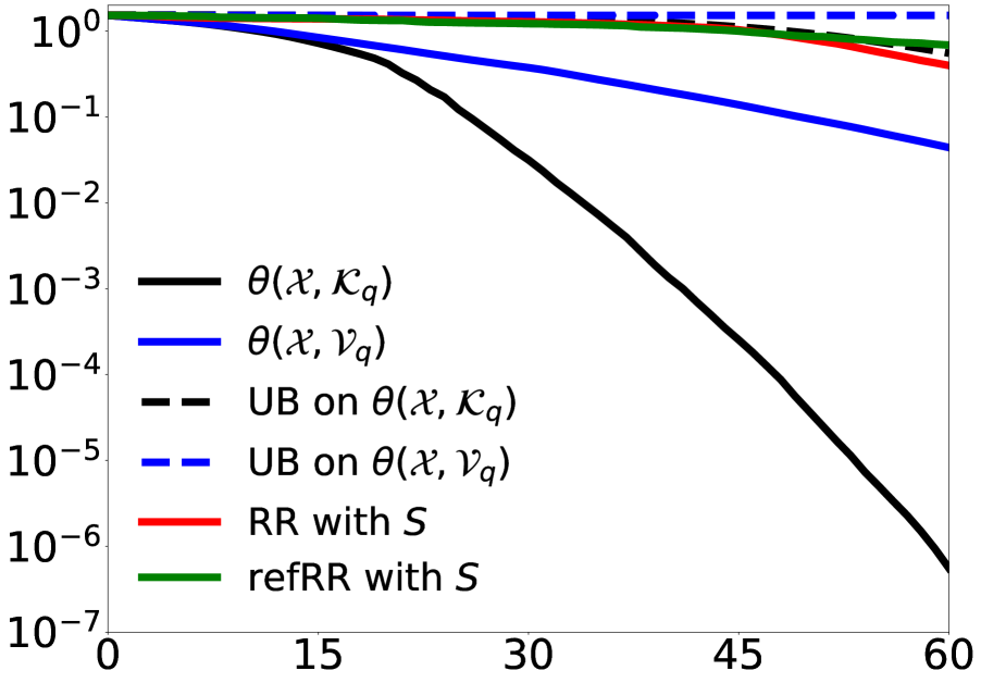
(a) $r=30$, $p=20$ and $G=0$

(b) $r=30$, $p=20$ and $G=10$

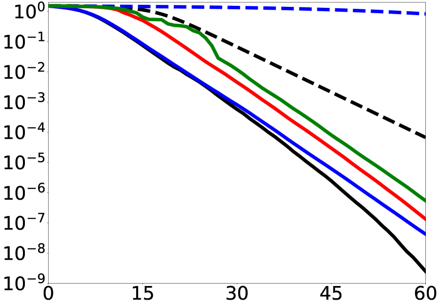
(c) $r=30$, $p=20$ and $G=70$

(d) $r=60$, $p=40$ and $G=0$

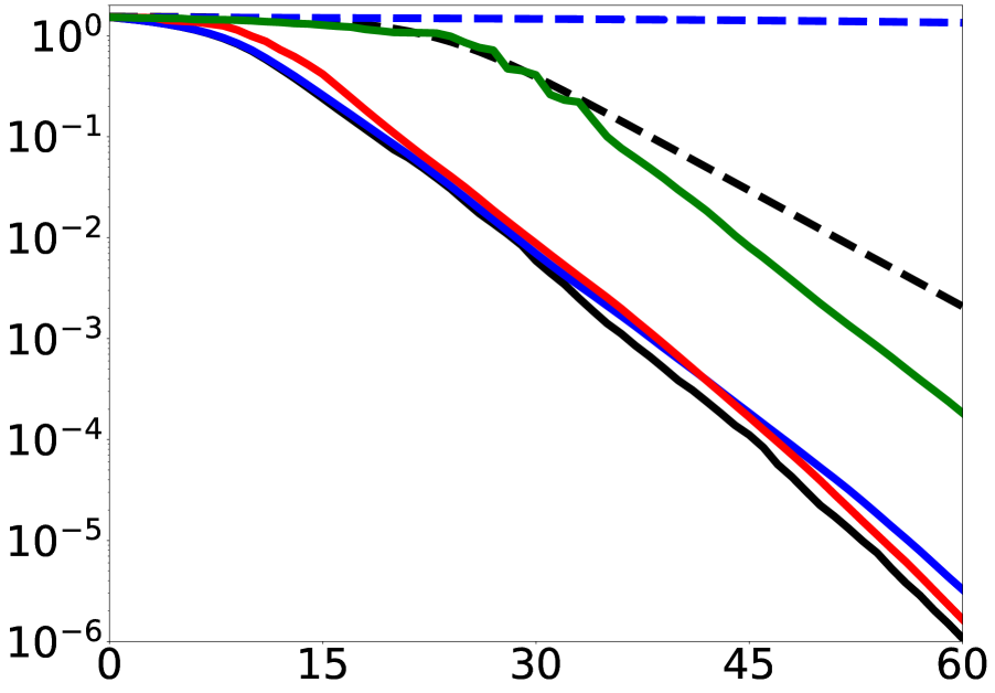
(e) $r=20$, $p=15$ and $G=40$

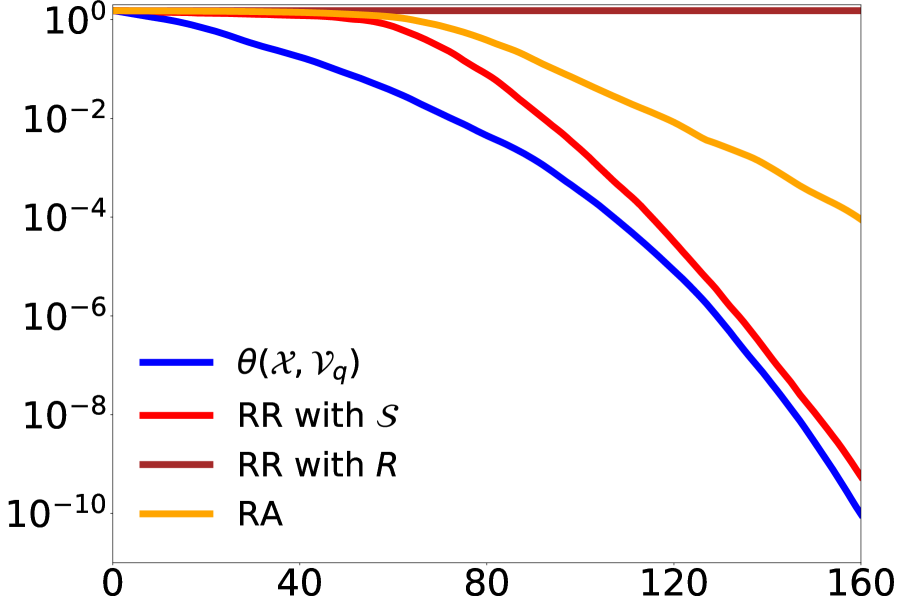
(f) $r=30$, $p=20$ and $G=0$

Figure 2: Linear decay models

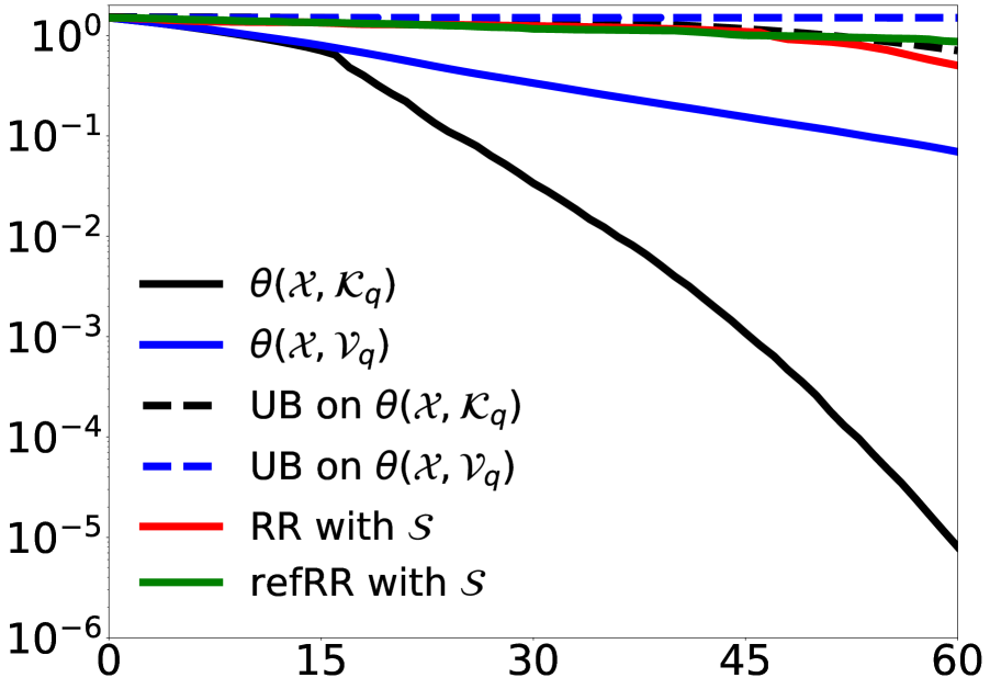
(a) $r=45$, $p=30$ and $G=0$

(b) $r=45$, $p=30$ and $G=0.005$

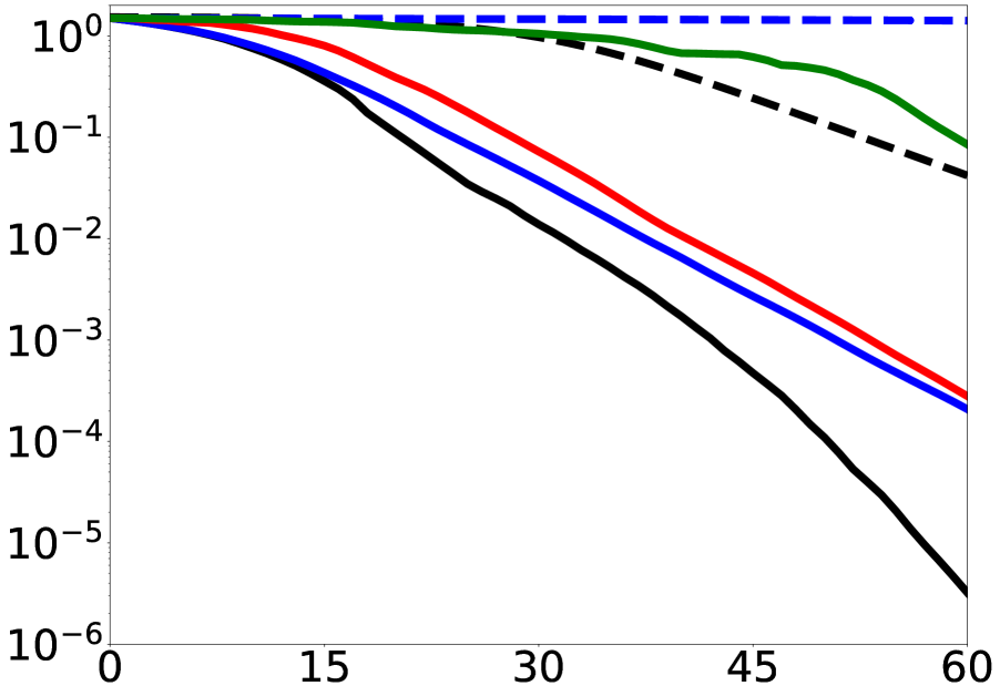
(c) $r=45$, $p=30$ and $G=0.02$

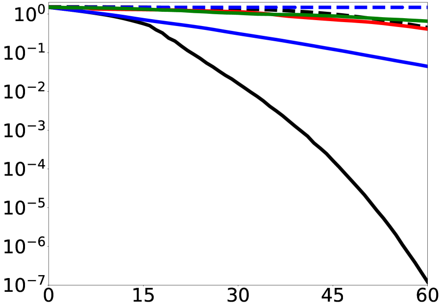
(d) $r=60,\,p=40$ and $G=0$

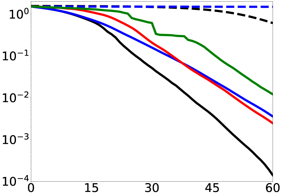
(e) $r=30,\,p=27$ and $G=0.01$

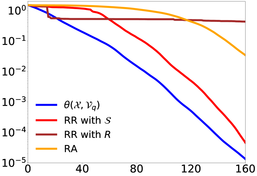
(f) $r=45,\,p=30$ and $G=0$

Figure 3: Eliptical decay models

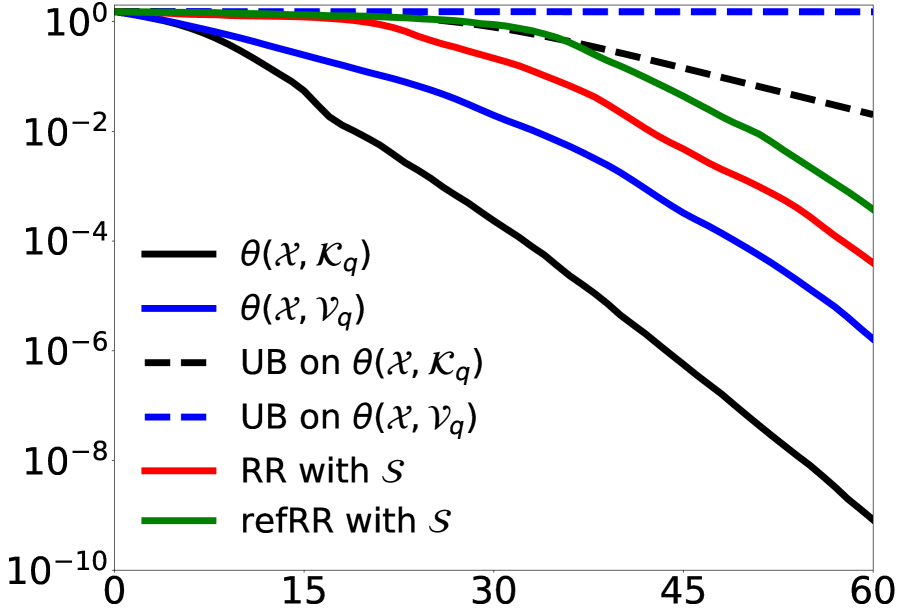
(a) $r=30,\,p=20$ and $G=0$

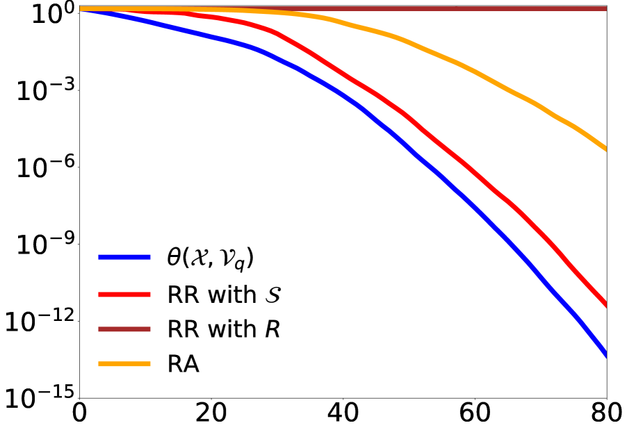
(b) $r=30,\,p=20$ and $G=0$

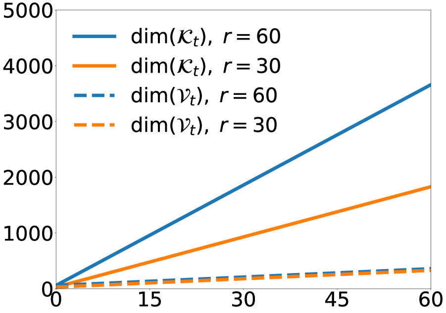
(c) Dimensions of various subspaces

Figure 4: Polynomial (baseline) decay model with moderate oversampling and various dimensions.

Analysis of the numerical results. In all the computed examples, the block Krylov method produces the best approximation of the target space $\mathcal{X}$ after 60 iterations. This is in accordance with the fact that ${\cal V}_{t}\subset\mathcal{K}_{t}$, for $0\leq t\leq q$, and that $\dim{\cal V}\geq\dim\mathcal{X}$ (see the comments after Theorem 3.8). On the other hand, the theoretical optimal subspace expansion computed by Algorithm 3.1 typically provides better approximations than its computable counterparts obtained using Algorithm 3.2, based on the RR and ref-RR methods.

The approximations of the target subspace based on the implementation of Algorithm 3.2 using the RR method typically have a better performance than those approximations obtained using the ref-RR method. Although the ref-RR method produces approximated eigenvectors that have smaller residual errors than those approximated eigenvectors obtained using the RR method [6, 8], this fact does not seem to imply that the subspaces computed using Algorithm 3.2 based on the ref-RR method have smaller angular distance that those computed using RR method. Furthermore, RR projection methods are considerably faster than ref-RR projection methods (for the same number of iterations). For these reasons we have not included the extension of Jia’s expansion method based on the refined Rayleigh-Ritz, but we point out that, for $q=60$, our experiments with the extension of Jia’s expansion method gave similar results for both projections methods.

The upper bound in Theorem 3.9 shows that both the decay of the eigenvalues values of the matrix $A$ and the oversampling ($\rho=r-d$) of the method play a role in the decay of the (largest) angle $\theta(\mathcal{X},\mathcal{K}_{t})$ as a function of the number of iterations $t\geq 0$ (see the comments after Theorem 3.9 and in Remark 3.10). These facts are reflected in the numerical examples: the faster the eigenvalues values decay or the larger the oversampling the faster the angles $\theta(\mathcal{X},\mathcal{K}_{t})$ decay, as a function of $t$. Figures 2(a) and 3(a) should be compared with Figures 2(d) and 3(d) respectively to get a grasp of the effects of oversampling in our experiments, keeping the same singular gap ($G=0$).

On the other hand, the upper bound in Theorem 3.8 shows that the gap between the eigenvalues $\lambda_{d}>\lambda_{d+1}$ of the matrix $A$ plays a role in the decay of the (largest) angle $\theta(\mathcal{X},{\cal V}_{t})$ as a function of $t\geq 0$. Notice that the previous analysis does not involve the oversampling of the method. The numerical examples confirm the role of the gap $\lambda_{d}>\lambda_{d+1}$ and also show a relatively small impact of the oversampling of the method in the decay of the angle $\theta(\mathcal{X},{\cal V}_{t})$, as a function of $0\leq t\leq q$.

Regarding the growth of the dimensions of the computed subspaces, we point out that in all the numerical examples we get that $\dim\mathcal{K}_{t}=(t+1)\cdot r$, while $\dim{\cal V}_{t}=\dim\widehat{\cal V}_{t}=r+t\cdot d$, for $0\leq t\leq q$. In particular, after $q=60$ iterations with $r=30$ ($d=5$ and $n=5000$) we have $\dim\mathcal{K}_{60}=1830$ ($\approx 36\%$ of $n=5000$) while $\dim{\cal V}_{60}=\dim\widehat{\cal V}_{60}=330$ ( $\approx 6\%$ of $n=5000$ and $\approx 18\%$ of $\dim\mathcal{K}_{60}$). These last facts are also reflected in the computational times of the different methods. Indeed, Algorithm 3.2 using the RR projection method becomes considerable faster than the block Krylov method as the number of iterations increases. For example, the computational time of block Krylov method for the elliptic model shown in Figure 3(a) (with $r=45$) is comparable with the computational time of the Algorithm 3.2 using the RR projection method shown in Figure 3(f). Moreover, $\theta(\mathcal{X},\,\mathcal{K}_{60})\approx\theta(\mathcal{X},\,\widehat{{\cal V}}_{160})$ while $\dim\mathcal{K}_{60}\approx 2700$ and $\dim\widehat{{\cal V}}_{160}\approx 850$. Similar comments apply to the linear model (Figures 2(a) and 2(f)) and the polynomial model (Figures 4(a) and 4(b)).

The performances of the theoretical optimal expansion ${\cal V}_{t}$ as well as its computable counterparts $\widehat{\cal V}_{t}$ are comparable with the block Krylov method (for the same number of iterations) in cases in which the eigenvalue gap $\lambda_{d}>\lambda_{d+1}$ is significant and the oversampling of the methods is rather small. In the example shown in Figure 2(e), after $q=60$ iterations we have that $\dim\mathcal{K}_{60}=1220$, while $\dim{\cal V}_{60}=\dim{\cal V}_{60}=320$ ($\approx 26\%$ of $\dim\mathcal{K}_{60}$).

6 Appendix: some technical results

In this section we present detailed proofs of the technical statements included in Section 4.

6.1 Principal angles between subspaces

Below we present the proofs of Propositions 4.1 and 4.2. Although these results are arguably folklore, we include their proofs for the convenience of the reader.

Proof of Proposition 4.1.

We consider subspaces $\mathcal{X},\,\mathcal{Y},\,{\cal S}\subset\mathbb{C}^{n}$, such that $d=\dim\mathcal{X}\leq\dim\mathcal{Y}$ and $\mathcal{Y}\subseteq{\cal S}$.

To show that $\Theta(\mathcal{X},\,{\cal S})\leq\Theta(\mathcal{X},\,\mathcal{Y})$ notice that $\mathcal{Y}\subseteq{\cal S}$, so we have that $P_{\cal S}P_{\mathcal{Y}}=P_{\mathcal{Y}}=P_{\mathcal{Y}}P_{\cal S}$. Then, for every $i\in\mathbb{I}_{d}\,$,

$$\begin{array}[]{rl}\cos^{2}(\theta_{i}(\mathcal{X},\,\mathcal{Y}))=s_{i}(P_{\mathcal{X}}P_{\mathcal{Y}})^{2}&=\lambda_{i}(P_{\mathcal{Y}}P_{\mathcal{X}}P_{\mathcal{Y}})=\lambda_{i}(P_{\mathcal{Y}}(P_{\cal S}P_{\mathcal{X}}P_{\cal S})P_{\mathcal{Y}})\\ &\\ &\stackrel{{\scriptstyle\star}}{{\leq}}\lambda_{i}(P_{\cal S}P_{\mathcal{X}}P_{\cal S})=s_{i}(P_{\mathcal{X}}P_{\cal S})^{2}=\cos^{2}(\theta_{i}(\mathcal{X},\,{\cal S}))\ ,\end{array}$$ (15)

where the inequalities $\stackrel{{\scriptstyle\star}}{{\leq}}$ follow by the interlacing inequalities. Thus, since the principal angles lay in $[0,\pi/2]$, the result follows from the fact that $\cos(x)$ is a decreasing function in that interval.

Denote by ${\cal M}=P_{\cal S}(\mathcal{X})\subseteq{\cal S}$ and $m=\dim{\cal M}\leq d$. Notice that since $P_{\cal M}P_{\mathcal{X}}=P_{\cal S}P_{\mathcal{X}}$ then $0<s_{i}(P_{\cal M}P_{\mathcal{X}})=s_{i}(P_{\cal S}P_{\mathcal{X}})=\cos(\theta_{i})$, for $1\leq i\leq m$. Furthermore, $s_{i}(P_{\cal S}P_{\mathcal{X}})=s_{i}(P_{\cal M}P_{\mathcal{X}})=0$ for $m<i\leq d$. These facts show that $\theta_{i}(\mathcal{X},{\cal M})\in[0,\pi/2)$ for $i\in\mathbb{I}_{m}$ and $\theta_{i}(\mathcal{X},{\cal M})=\pi/2$ for $m+1\leq i\leq d$, which is item 2.

By the case of equality in the interlacing inequalities in Eq. (15), we get that $\Theta(\mathcal{X},{\cal S})=\Theta(\mathcal{X},\mathcal{Y})$ (that is $\lambda_{i}(P_{\mathcal{Y}}P_{\mathcal{X}}P_{\mathcal{Y}})=\lambda_{i}(P_{\cal S}P_{\mathcal{X}}P_{\cal S})$, for $1\leq i\leq d$) if and only if $\mathcal{Y}$ contains an orthonormal system $\{y_{1},\ldots,y_{d}\}$ such that

$$P_{\cal S}P_{\mathcal{X}}P_{\cal S}\ y_{i}=\cos^{2}(\theta_{i}(\mathcal{X},{\cal S})\,)\ y_{i}\quad\text{ for every }\quad i\in\mathbb{I}_{d}\ .$$

Since $\cos(\theta_{i}(\mathcal{X},{\cal S})\,)>0$ for $i\in\mathbb{I}_{m}\,$, this means that $\{y_{1},\ldots,y_{m}\}\subseteq P_{\cal S}(\mathcal{X})={\cal M}$ (and they form an orthonormal basis for ${\cal M}$). Hence $\Theta(\mathcal{X},{\cal S})=\Theta(\mathcal{X},\mathcal{Y})$ if and only if ${\cal M}\subseteq\mathcal{Y}$ which is item 3. $\square$

Proof of Proposition 4.2.

Let ${\cal V}\,,\,\mathcal{A}\subseteq\mathbb{C}^{n}$ be subspaces and set ${\cal S}={\cal V}+\mathcal{A}$. To prove Eq. (10) i.e. ${\cal S}={\cal V}+\mathcal{A}={\cal V}\oplus(1-P_{\cal V})(\mathcal{A})$, let $v+a\in{\cal V}+\mathcal{A}$, for some $v\in{\cal V}$ and $a\in\mathcal{A}$. Then

$$v+a=P_{\cal V}(v+a)+(1-P_{\cal V})(v+a)=v^{\prime}+(1-P_{\cal V})a\in{\cal V}\oplus(1-P_{\cal V})(\mathcal{A})\ ,$$

where $v^{\prime}=P_{\cal V}(v+a)$ and where we used that $(1-P_{\cal V})v=0$. Conversely, if $v\in{\cal V}$ and $a\in\mathcal{A}$ then $v+(1-P_{\cal V})a=v+(a-P_{\cal V}a)=v^{\prime}+a$, where $v^{\prime}=v-P_{\cal V}a\in{\cal V}$.

Given a subspace $\mathcal{E}$ such that ${\cal V}\subseteq\mathcal{E}\subseteq{\cal S}$, simply take $\mathcal{D}=\mathcal{A}\cap\mathcal{E}\subseteq\mathcal{A}$, which clearly satisfies that ${\cal V}+\mathcal{D}\subseteq\mathcal{E}$. Moreover, given $e\in\mathcal{E}\subseteq{\cal S}$ there exists $a\in\mathcal{A}$ and $v\in{\cal V}$ such that $a=e-v\in\mathcal{D}$ so $e=v+a\in{\cal V}+\mathcal{D}$. We therefore conclude that $\mathcal{E}={\cal V}+\mathcal{D}\stackrel{{\scriptstyle\eqref{eq desc sum1}}}{{=}}{\cal V}+(1-P_{{\cal V}})\mathcal{D}$. $\square$

6.2 Principal angles and their tangents

In this section we prove a key inequality involving tangents of principal angles between subspaces, that is related with the work in [28]. Indeed, if we let $\begin{bmatrix}X&X_{\bot}\end{bmatrix}$ be a unitary matrix with $X\in\mathbb{C}^{n\times d}$ and $V\in\mathbb{C}^{n\times r}$ with orthonormal columns and such that $\text{\rm rk}(X^{*}V)=d$ then, the first $d$ singular values of $X_{\bot}^{*}V(X^{*}V)^{\dagger}$ coincide with the tangents of the angles between $R(X)$ and $R(V)$. In case that $V$ does not have orthonormal columns then the situation changes, as shown in the following

Example 6.1.

Let $\begin{bmatrix}X&X_{\bot}\end{bmatrix}$ be the identity matrix of size 5, with $X\in\mathbb{C}^{5\times 2}$, and $\{V_{a}\}_{a\in\mathbb{R}}$ be the family of matrices given by

$$V_{a}=\frac{1}{\sqrt{2}}\begin{pmatrix}1&0&0\\ 0&1&0\\ 1&0&0\\ 0&1&0\\ a&0&\sqrt{2}\end{pmatrix}\in\mathbb{C}^{5\times 3}\,.$$

It’s easy to see that $\text{\rm rk}(V_{a})=3$, $\text{\rm rk}(X^{*}V_{a})=2$ and $R(V_{a})=R(V_{0})$ for all $a\in\mathbb{R}$, but

$$X_{\bot}^{*}V_{a}(X^{*}V_{a})^{\dagger}=\begin{pmatrix}1&0&0\\ 0&1&0\\ a&0&\sqrt{2}\end{pmatrix}\begin{pmatrix}1&0&0\\ 0&1&0\end{pmatrix}^{\dagger}=\begin{pmatrix}1&0\\ 0&1\\ a&0\end{pmatrix}\Longrightarrow s(X_{\bot}^{*}V_{a}(X^{*}V_{a})^{\dagger})=((1+a^{2})^{1/2},1)\,.$$

So, the matrices $V_{a}$ are all full rank and they all have the same range, but the matrices $X_{\bot}^{*}V_{a}(X^{*}V_{a})^{\dagger}$ may have an arbitrarily large first singular value, which doesn’t contradict [28, Theorem 3.1], since $\text{\rm rk}(V_{a})=3>2=\text{\rm rk}(X^{*}V_{a})$. Notice that the choice $a=0$ produces the smallest singular values, which is exactly the case where the matrix $V_{a}$ has orthonormal columns. In that case, those singular values coincide with the tangents of the angles $\theta(X,\,V)$. $\triangle$

The next result, that complements the result from Zhu and Knyazev, will play a key role in our approach to the convergence analysis of Algorithm 3.1 in the Hermitian case. Notice that the next result is stronger than Theorem 4.5.

Theorem 6.2.

Let $\begin{bmatrix}X&X_{\bot}\end{bmatrix}$ be a unitary matrix with $X\in\mathbb{C}^{n\times d}$ and let $V\in\mathbb{C}^{n\times r^{\prime}}$ be such that $X^{*}V\neq 0$. Let $V_{0}\in\mathbb{C}^{n\times r}$ have orthonormal columns and be such that $R(V)=R(V_{0})={\cal V}$. Then, we have that

$$s_{j}(X_{\bot}^{*}V_{0}(X^{*}V_{0})^{\dagger})\leq s_{j}(X_{\bot}^{*}V(X^{*}V)^{\dagger})\ ,\ \text{ for}\ 1\leq j\leq d\,.$$

If we assume further that $\dim X^{*}({\cal V})=d$ (so $r\geq d$) then,

$$s_{j}(\tan(\Theta(\mathcal{X},\,{\cal V})))\leq s_{j}(X_{\bot}^{*}V(X^{*}V)^{\dagger})\ \text{ for}\ 1\leq j\leq d\,,$$ (16)

where $\mathcal{X}=R(X)$. In particular, for every unitary invariant norm $\|\cdot\|$ we have that

$$\|X_{\bot}^{*}V_{0}(X^{*}V_{0})^{\dagger}\|=\|\tan(\Theta(\mathcal{X},{\cal V}))\|\leq\|X_{\bot}^{*}V(X^{*}V)^{\dagger}\|\,.$$

Proof.

We first show that we can reduce our analysis to the case in which $\mathcal{X}\cap{\cal V}^{\perp}=\{0\}$ or, equivalently, that $\dim X^{*}({\cal V})=d$. Indeed, let $V\in\mathbb{C}^{n\times r^{\prime}}$ be such that ${\cal V}=R(V)$. Let $\mathcal{X}\cap{\cal V}^{\perp}=\mathcal{X}_{1}$ and notice that by hypothesis $\dim\mathcal{X}_{1}<d$. Assume further that $1\leq\dim\mathcal{X}_{1}=d_{1}$ and set $\mathcal{X}_{2}=\mathcal{X}\ominus\mathcal{X}_{1}$. Since $\text{\rm rk}(X^{*}V)=d-d_{1}$, we have that $s_{j}(X_{\bot}^{*}V(X^{*}V)^{\dagger})=0$ for $j>d-d_{1}$. Replacing $[X\ \ X_{\perp}]$ by $[X\ \ X_{\perp}]=[XW\ \ X_{\perp}]$ for a convenient unitary matrix $W\in\mathbb{C}^{d\times d}$ we can further assume that $X=[X_{1}\ \ X_{2}]$, where $X_{1}$ and $X_{2}$ have columns that form orthonormal basis of $\mathcal{X}_{1}$ and $\mathcal{X}_{2}$, respectively. We remark that this replacement does not modify $s(X_{\bot}^{*}V(X^{*}V)^{\dagger})$. Then,

$$X^{*}V=\begin{bmatrix}X_{1}^{*}\\ X_{2}^{*}\end{bmatrix}V=\begin{bmatrix}0\\ X_{2}^{*}V\end{bmatrix}\implies(X^{*}V)^{\dagger}=[0\ \ (X_{2}V)^{\dagger}]\,.$$

Hence, $X_{\perp}^{*}V(X^{*}V)^{\dagger}=X_{\perp}^{*}V[0\ \ (X_{2}V)^{\dagger}]=[0\ \ X_{\perp}^{*}V(X_{2}V)^{\dagger}]$. Notice that the columns of the matrix $\tilde{U}=[X_{2}\ \ X_{\perp}]\in\mathbb{C}^{n\times(n-d_{1})}$ form an orthonormal basis of $\mathbb{C}^{n}\ominus\mathcal{X}_{1}=\mathcal{X}_{2}\oplus\mathcal{X}^{\perp}$. Consider $I_{n-d_{1}}=\tilde{U}^{*}\tilde{U}=[H_{1}\ \ H_{1,\perp}]\in\mathbb{C}^{(n-d_{1})\times(n-d_{1})}$, where the columns of $H_{1}$ and $H_{1,\perp}$ are the first $d-d_{1}$ and last $n-d$ vectors of the canonical basis of $\mathbb{C}^{n-d_{1}}$ and set $\tilde{V}:=\tilde{U}^{*}V\in\mathbb{C}^{(n-d_{1})\times r^{\prime}}$. By construction we have that $X_{1}^{*}V=0$ and $\tilde{U}\,{\tilde{U}}^{*}=I_{n}-X_{1}X_{1}^{*}$ and thus, $\tilde{U}\,\tilde{V}=(I_{n}-X_{1}X_{1}^{*})V=V$. Since $\tilde{U}$ has orthonormal columns

$$\tilde{U}(R(\tilde{V})^{\perp})=[\tilde{U}(R(\tilde{V}))]^{\perp}\ominus\mathcal{X}_{1}={\cal V}^{\perp}\ominus\mathcal{X}_{1}\,.$$

We also have that

$$\tilde{U}(R(H_{1})\cap R(\tilde{V})^{\perp})=\tilde{U}(R(H_{1}))\cap\tilde{U}(R(\tilde{V})^{\perp})=\mathcal{X}_{2}\cap({\cal V}^{\perp}\ominus\mathcal{X}_{1})=\{0\}\,.$$

Thus, $R(H_{1})\cap R(\tilde{V})^{\perp}=\{0\}$. Moreover, we get that $H_{1,\perp}^{*}\tilde{V}(H_{1}^{*}\tilde{V})^{\dagger}=X_{\perp}^{*}V(X_{2}^{*}V)^{\dagger}$. The previous facts show that

$$s_{j}(X_{\perp}^{*}V(X^{*}V)^{\dagger})=s_{j}(H_{1,\perp}^{*}\tilde{V}(H_{1}^{*}\tilde{V})^{\dagger})\ ,\ \text{ for}\ 1\leq j\leq d-d_{1}\,.$$

Thus, we can replace the triplet $(X,X_{\perp},V)$ by $(H_{1},H_{1,\perp},\tilde{V})$ in such a way that $R(H_{1})\cap R(\tilde{V})^{\perp}=\{0\}$. Notice that $\tilde{U}$, $H_{1}$ and $H_{1,\perp}$ only depend on $[X\ \ X_{\perp}]$ and ${\cal V}$; also notice that $\tilde{V}=\tilde{U}^{*}V$ has orthonormal columns whenever $V$ has orthonormal columns. Thus, in what follows we assume further that $\mathcal{X}\cap{\cal V}^{\perp}=\{0\}$ or equivalently, that $\dim X^{*}({\cal V})=d$.

Under this assumption, it follows from [28, Theorem 3.1] that $s_{j}(X_{\perp}^{*}V_{0}(X^{*}V_{0})^{\dagger})$ is equal to $s_{j}(\tan(\Theta(\mathcal{X},\,{\cal V})))$, for $1\leq j\leq d$. Thus, if we prove the singular value inequalities in Eq. (16) then the first set of inequalities will follow. Also, by means of Ky Fan’s dominance theorem (see [1, Theorem IV.2.2]) Eq. (16) also implies the last inequality in the statement, so we are only left to prove Eq. (16)

By the previous argument we now consider a unitary matrix $[X\ \ X_{\perp}]\in\mathbb{C}^{n\times n}$ and $V\in\mathbb{C}^{n\times r^{\prime}}$ such that if ${\cal V}=R(V)$ and $\mathcal{X}=R(X)$ then $\mathcal{X}\cap{\cal V}^{\perp}=\{0\}$. Next we show that we can further assume that $V$ has full column rank. Indeed, we can always choose an orthonormal basis $\{w_{1},\ldots,w_{r}\}\subseteq\mathbb{C}^{r^{\prime}}$ for $\ker(V)^{\perp}$ and another orthonormal basis $\{w_{r+1},\ldots,w_{r^{\prime}}\}\subseteq\mathbb{C}^{r^{\prime}}$ for $\ker(V)$ to produce a unitary matrix $W=[w_{1}\cdots w_{r^{\prime}}]\in\mathbb{C}^{r^{\prime}\times r^{\prime}}$ and consider $VW$. Notice that $VW=\begin{bmatrix}V_{1}&0\end{bmatrix}$ where $V_{1}\in\mathbb{C}^{n\times r}$ has full column rank and the same range as $V$, so the LHS of Eq. (16) remains the same when we replace $V$ with $V_{1}$. We now need to show that this is also the case for the RHS of Eq. (16), which is done directly:

$$X_{\bot}^{*}V(X^{*}V)^{\dagger} =X_{\bot}^{*}VW\;W^{*}(X^{*}V)^{\dagger}=X_{\bot}^{*}VW\;(X^{*}VW)^{\dagger}$$

$$=X_{\bot}^{*}\begin{bmatrix}V_{1}&0\end{bmatrix}\;(X^{*}\begin{bmatrix}V_{1}&0\end{bmatrix})^{\dagger}=\begin{bmatrix}X_{\bot}^{*}V_{1}&0\end{bmatrix}\;\begin{bmatrix}X^{*}V_{1}&0\end{bmatrix}^{\dagger}$$

$$=\begin{bmatrix}X_{\bot}^{*}V_{1}&0\end{bmatrix}\;\begin{bmatrix}(X^{*}V_{1})^{\dagger}\\ 0\end{bmatrix}=X_{\bot}^{*}V_{1}(X^{*}V_{1})^{\dagger}$$

since $W$ is unitary. Thus, we further assume (for now) that $V=V_{1}$ is full column rank and that $r^{\prime}=r$.

Let ${\cal S}=\ker(X^{*}V)$: our assumptions imply that ${\cal S}\subseteq\mathbb{C}^{r}$, $\dim{\cal S}=r-d$ and that $\dim V({\cal S}^{\bot})=\dim{\cal S}^{\perp}=d$, where we used that $V$ is full column rank. Hence, by item 1. in Proposition 4.1, we have that $\Theta(X,\,V)\leq\Theta(X,\,V({\cal S}^{\bot}))$. This implies that, for $1\leq j\leq d$

$$s_{j}(\tan(\Theta(X,\,V)))\leq s_{j}(\tan(\Theta(X,\,V({\cal S}^{\bot}))))\,.$$ (17)

If we let $\tilde{V}=VP_{{\cal S}^{\bot}}$, then $R(\tilde{V})=V({\cal S}^{\perp})$, so $\text{\rm rk}(\tilde{V})=d$, and $X^{*}\tilde{V}=X^{*}VP_{{\cal S}^{\bot}}=X^{*}V$, so

$$\ker(X^{*}\tilde{V})=\ker(X^{*}V)={\cal S}=\ker(\tilde{V})\,.$$

Using the fact that $R((X^{*}V)^{\dagger})=\ker(X^{*}V)^{\bot}={\cal S}^{\bot}$ we have that

$$X_{\bot}^{*}\tilde{V}(X^{*}\tilde{V})^{\dagger}=X_{\bot}^{*}VP_{{\cal S}^{\bot}}(X^{*}VP_{{\cal S}^{\bot}})^{\dagger}=X_{\bot}^{*}V(X^{*}V)^{\dagger}\,,$$ (18)

and combining (17) with (18) it is easy to see that if we can prove that (16) holds for $\tilde{V}$ then it also holds for $V$. To save notation, we will write $V$ instead of $\tilde{V}$, dropping the assumption that $V$ has full column rank and assuming that it satisfies the following conditions: $\ker(X^{*}V)=\ker V$ and $\text{\rm rk}(V)=\text{\rm rk}(X^{*}V)=d$.

Let us take the polar decomposition $V=U|V|$ of $V$; in this case $U\in\mathbb{C}^{n\times r}$ is a partial isometry (i.e. $UU^{*}=P_{R(U)}$ and $U^{*}U=P_{\ker(U)^{\perp}}$) such that $R(U)=R(V)$ and $\ker U=\ker V=\ker(X^{*}V)$. Since $R(U)=R(V)$ we have that $R(X^{*}U)=R(X^{*}V)$, so $\text{\rm rk}(X^{*}U)=d$. Moreover, $\ker(X^{*}U)=\ker(U)$: Indeed, the inclusion $\ker(U)\subset\ker(X^{*}U)$ is trivial and the dimensions coincide:

$$\dim\ker(X^{*}U)=r-\text{\rm rk}(X^{*}U)=r-\text{\rm rk}(X^{*}V)=r-\text{\rm rk}(V)=r-\text{\rm rk}(U)=\dim\ker(U)\,.$$

Now, consider a SVD of $X^{*}U$ given by $X^{*}U=Z\Sigma W^{*}$, where $Z\in\mathbb{C}^{d\times d}$ and $W\in\mathbb{C}^{r\times r}$ are unitary matrices. Let $\{z_{1},\ldots,z_{d}\}$ and $\{w_{1},\ldots,w_{d}\}$ denote the first $d$ columns of $Z$ and $W$ respectively. Notice that $\{w_{1},\ldots,w_{d}\}$ is a basis for the subspace $\ker(X^{*}U)^{\perp}=\ker(U)^{\bot}=\ker(V)^{\bot}=\ker(X^{*}V)^{\bot}$ and

$$X^{*}Uw_{i}=\cos(\theta_{i})\ z_{i}\ ,\ 1\leq i\leq d$$

where $\theta_{i}=\theta_{i}(X,\,V)$, for $1\leq i\leq d$. Taking the adjoint of the previous SVD we get $U^{*}X=W\Sigma Z^{*}$ so

$$U^{*}Xz_{i}=\cos(\theta_{i})\ w_{i}\ ,\ 1\leq i\leq d\,.$$

Using the fact that $R(|V|^{\dagger})=R(|V|)=\ker V^{\perp}=\ker U^{\perp}=(\ker X^{*}V)^{\perp}$ we get that

$$\cos(\theta_{i})\ z_{i}=X^{*}U|V|\ |V|^{\dagger}w_{i}=X^{*}V(|V|^{\dagger}w_{i})\Rightarrow\cos(\theta_{i})(X^{*}V)^{\dagger}z_{i}=|V|^{\dagger}w_{i}$$

and it follows that

$$X_{\bot}^{*}V(X^{*}V)^{\dagger}z_{i}=\frac{1}{\cos(\theta_{i})}X_{\bot}^{*}U|V||V|^{\dagger}w_{i}=\frac{1}{\cos(\theta_{i})}X_{\bot}^{*}Uw_{i}\ ,\ 1\leq i\leq d\,.$$

Next, notice that $\{w_{i}\}_{1\leq i\leq d}\subseteq\ker U^{\bot}$, where $\begin{bmatrix}X&X_{\bot}\end{bmatrix}^{*}U$ acts isometrically. So, the vectors

$$\begin{bmatrix}X&X_{\bot}\end{bmatrix}^{*}Uw_{i}=\begin{bmatrix}X^{*}Uw_{i}\\ X_{\bot}^{*}Uw_{i}\end{bmatrix}=\begin{bmatrix}\cos(\theta_{i})z_{i}\\ X_{\bot}^{*}Uw_{i}\end{bmatrix}\text{ for }1\leq i\leq d$$

form an orthonormal system. From this (and the fact $\{z_{i}\}_{1\leq i\leq d}$ is an orthonormal system) we deduce that $\{X_{\bot}^{*}Uw_{i}\}_{1\leq i\leq d}$ is an orthogonal system with $\|X_{\bot}^{*}Uw_{i}\|=\sin(\theta_{i})$, for $1\leq i\leq d$.

We now consider the following variational characterization of the singular values (see [1, Problem III.6.1]): if we let ${\cal M}_{j}$ be the $j$-dimensional subspace spanned by $\{z_{i}\,:\,d-j+1\leq i\leq d\}$ then, for $1\leq j\leq d$ we have that

$$s_{j}^{2}(X_{\bot}^{*}V(X^{*}V)^{\dagger}) \geq\min_{x\in{\cal M}_{j},\;\|x\|=1}\|X_{\bot}^{*}V(X^{*}V)^{\dagger}x\|^{2}$$

$$=\min_{\sum_{i=d-j+1}^{d}|\alpha_{i}|^{2}=1}\left\|\sum_{i=d-j+1}^{d}\frac{\alpha_{i}}{\cos(\theta_{i})}X_{\bot}^{*}Uw_{i}\right\|^{2}$$

$$=\min_{\sum_{i=d-j+1}^{d}|\alpha_{i}|^{2}=1}\sum_{i=d-j+1}^{d}\frac{|\alpha_{i}|^{2}}{\cos^{2}(\theta_{i})}\|X_{\bot}^{*}Uw_{i}\|^{2}$$

$$=\min_{\sum_{i=d-j+1}^{d}|\alpha_{i}|^{2}=1}\sum_{i=d-j+1}^{d}|\alpha_{i}|^{2}\tan^{2}(\theta_{i})$$

$$\geq\tan^{2}(\theta_{d-j+1})=s_{j}^{2}(\tan(\Theta(X,V)))\,.$$

Taking square roots on both sides, the proof is complete.

∎

6.3 Analysis of iterative algorithms

Proof of Theorem 4.6.

We fix an Hermitian matrix $A\in\mathbb{C}^{n\times n}$ and consider an eigen-decomposition $A=X\Lambda X^{*}$ , where the matrix $X\in\mathbb{C}^{n\times n}$ is unitary and $\Lambda=\text{diag}(\lambda_{1},\ldots,\lambda_{n})$, with $\lambda_{1}\geq\ldots\geq\lambda_{n}$. We let $x_{1},\ldots,x_{n}$ denote the columns of $X$. Hence, $A\,x_{j}=\lambda_{j}\,x_{j}$, for $1\leq j\leq n$. We assume further that $\lambda_{d}>\lambda_{d+1}$. Furthermore, for $1\leq\ell\leq n$ we consider the partitions:

$$X=\begin{bmatrix}X_{\ell}&X_{\ell,\bot}\end{bmatrix}\quad\text{ and }\quad\Lambda=\begin{bmatrix}\Lambda_{\ell}&0\\ 0&\Lambda_{\ell,\bot}\end{bmatrix}\,.$$

where $X_{\ell}\in\mathbb{C}^{n\times\ell}$ and $\Lambda_{\ell}\in\mathbb{C}^{\ell\times\ell}$.

We let ${\cal V}\subset\mathbb{C}^{n}$ with $\dim{\cal V}=r\geq d$ and fix $d\leq p\leq r$ such that $\text{span}\{x_{1},\ldots,x_{p}\}\cap{\cal V}^{\perp}=\{0\}$. In what follows we find $\mathcal{H}_{p}\subset R(V)$ with $\dim\mathcal{H}_{p}=d+r-p$ such that

$$\|\tan(\Theta(\mathcal{X},\,\phi(A)({\cal V})))\|\leq\|\phi(\Lambda_{d})^{-1}\|_{2}\ \|\phi(\Lambda_{p,\perp})\|_{2}\;\|\tan(\Theta(\mathcal{X},\,\mathcal{H}_{p}))\|$$

for every polynomial $\phi\in\mathbb{C}[x]$ such that $\phi(\Lambda_{d})$ is invertible and for every u.i.n. $\|\cdot\|$.

Indeed, let $W\in\mathbb{C}^{n\times r}$ be a matrix with orthonormal columns such that $R(W)={\cal V}$. Since $\text{span}\{x_{1},\ldots,x_{p}\}\cap{\cal V}^{\perp}=\{0\}$ we get that $p=\text{\rm rk}(W^{*}X_{p})=\text{\rm rk}(X_{p}^{*}W)$. We now consider the matrix $F=[x_{d+1}\cdots x_{p}]^{*}W\in\mathbb{C}^{(p-d)\times r}$. The fact that $\text{\rm rk}(X_{p}^{*}W)=p$ implies that $\text{\rm rk}(F)=p-d$ so $\dim\ker(F)=r-(p-d)$. Let $Z\in\mathbb{C}^{r\times(d+r-p)}$ be such that it has orthonormal columns and $R(Z)=\ker(F)$. Then, $WZ\in\mathbb{C}^{n\times(d+r-p)}$ has orthonormal columns and is such that $R(WZ)\subset\{x_{d+1},\ldots,x_{p}\}^{\perp}$. Also, $R(WZ)\subset R(W)={\cal V}$ and $\text{\rm rk}(WZ)=d+r-p\geq d$. We define $\mathcal{H}_{p}=R(WZ)$ and check that this subspace has the desired properties. Indeed, the previous comments show that $\mathcal{H}_{p}\subset{\cal V}$ is such that $\dim\mathcal{H}_{p}=d+r-p$.

Since $\dim\ker(X_{p}^{*}W)^{\perp}=p$ we see that $\dim R(Z)+\dim\ker(X_{p}^{*}W)^{\perp}=d+(r-p)+p=r+d$ so we must have $\dim\ker(X_{p}^{*}W)^{\perp}\cap R(Z)\geq d$ so then $\text{\rm rk}(X_{p}^{*}WZ)\geq d$. But, by construction,

$$X_{p}^{*}WZ=[[x_{1}\cdots x_{d}]\ [x_{d+1}\cdots x_{p}]]^{*}WZ=\begin{bmatrix}X_{d}^{*}WZ\\ 0\end{bmatrix}\,.$$

Therefore, we conclude that $\text{\rm rk}(X_{d}^{*}WZ)=d$. Since $WZ$ has orthonormal columns, $R(WZ)=\mathcal{H}_{p}$ and $\dim\mathcal{H}_{p}\geq\dim\mathcal{X}$, we conclude that $\mathcal{X}\cap\mathcal{H}_{p}^{\perp}=\{0\}$.

Using the previous facts we can see, since $\phi(\Lambda_{d})$ is invertible, that $\text{\rm rk}(\phi(A)WZ)\geq d$. Also, $R(\phi(A)WZ)\subset R(\phi(A)W)=\phi(A)({\cal V})$. Thus, using item 1. in Proposition 4.1 and Theorem 4.5 we have that ($R(X_{d})=\mathcal{X}$)

$$\|\tan(\Theta(\mathcal{X},\phi(A)({\cal V})))\| =\|\tan(\Theta(\mathcal{X},\,\phi(A)W))\|$$

$$\leq\|\tan(\Theta(\mathcal{X},\,\phi(A)WZ))\|$$

$$\leq\|X_{d,\bot}^{*}\phi(A)WZ\;(X_{d}^{*}\phi(A)WZ)^{\dagger}\|$$

$$=\|X_{d,\bot}^{*}X\phi(\Lambda)X^{*}WZ\;(X_{d}^{*}X\phi(\Lambda)X^{*}WZ)^{\dagger}\|\,.$$

Now, we can simplify

$$X_{d,\bot}^{*}X\phi(\Lambda)X^{*}WZ=\phi(\Lambda_{d,\bot})X_{d,\bot}^{*}WZ=MX_{d,\bot}^{*}WZ\,,$$

where $M=\begin{bmatrix}0_{p-d}&0\\ 0&\phi(\Lambda_{p,\bot})\end{bmatrix}$ by using the fact that $X_{d,\bot}^{*}WZ=[0\ X_{p,\bot}]^{*}WZ$ by construction of $Z$. Similarly,

$$X_{d}^{*}X\phi(\Lambda)X^{*}WZ=\phi(\Lambda_{d})X_{d}^{*}WZ\,.$$

Using these identities in our previous estimation and using the fact that $\phi(\Lambda_{d})$ is invertible and $X_{d}^{*}WZ$ has full row rank, we obtain

$$\|\tan(\Theta(\mathcal{X},\,\phi(A)({\cal V})))\| \leq\|MX_{d,\bot}^{*}WZ(\phi(\Lambda_{d})X_{d}^{*}WZ)^{\dagger}\|$$

$$=\|MX_{d,\bot}^{*}WZ(X_{d}^{*}WZ)^{\dagger}\phi(\Lambda_{d})^{-1}\|\,.$$

Finally, by the strong sub-multiplicativity of the unitarily invariant norms we can conclude that

$$\|\tan(\Theta(\mathcal{X},\,\phi(A)({\cal V})))\| \leq\|MX_{d,\bot}^{*}WZ(X_{d}^{*}WZ)^{\dagger}\phi(\Lambda_{d})^{-1}\|$$

$$\leq\|M\|_{2}\;\|X_{d,\bot}^{*}WZ(X_{d}^{*}WZ)^{\dagger}\|\;\|\phi(\Lambda_{d})^{-1}\|_{2}$$

$$=\|\phi(\Lambda_{p,\bot})\|_{2}\;\|\tan(\Theta(\mathcal{X},\,\mathcal{H}_{p}))\|\;\|\phi(\Lambda_{d})^{-1}\|_{2}$$

where we have used Zhu and Knyazev’s result from [28] in the last identity, since $WZ$ and $X_{d}$ have orthonormal columns, $R(WZ)=\mathcal{H}_{p}$, $R(X_{d})=\mathcal{X}$ and $\text{\rm rk}(X_{d}^{*}WZ)=d$ (see the discussion at the beginning of Section 6.2). Hence, the subspace $\mathcal{H}_{p}$ has the desired properties. $\square$

The next technical lemma is needed for the proof of item $1.$ in Proposition 4.7.

Lemma 6.3.

Suppose that $\lambda_{1}\geq\ldots,\geq\lambda_{d}>\lambda_{d+1}\geq\ldots\geq\lambda_{n}=0$ are non negative real numbers and define $f:\mathbb{R}\setminus\{\lambda_{1},\ldots,\lambda_{d}\}\rightarrow\mathbb{R}$ as

$$f(s)=\left(\min_{1\leq j\leq d}|s-\lambda_{j}|\right)^{-1}\;\max_{d+1\leq j\leq n}|s-\lambda_{j}|\,.$$

Then, f achieves it’s absolute minimum at $s=\lambda_{d+1}/2$ and that minimun value is less than the singular gap $\lambda_{d+1}/\lambda_{d}<1$.

Proof.

Let $m=\lambda_{d+1}/2$. We first show that $f(m)$ is strictly less than the singular gap:

$$f(m)=\frac{1}{\lambda_{d}-\left(\frac{\lambda_{d+1}}{2}\right)}\;\frac{\lambda_{d+1}}{2}=\frac{\lambda_{d+1}}{\lambda_{d}+(\lambda_{d}-\lambda_{d+1})}<\frac{\lambda_{d+1}}{\lambda_{d}}$$

Now, to show that this is the minimum value of $f$, we consider the following cases:

1. If $s<m$ then, since $\lambda_{d+1}-\lambda_{d}<0$ we have that

   $$f(s)=\frac{\lambda_{d+1}-s}{\lambda_{d}-s}=1+\frac{\lambda_{d+1}-\lambda_{d}}{\lambda_{d}-s}>1+\frac{\lambda_{d+1}-\lambda_{d}}{\lambda_{d}-m}=\frac{\lambda_{d+1}-m}{\lambda_{d}-m}=f(m)\,.$$

2. If $s\in(m,\,\lambda_{d})$ then,

   $$f(s)=\frac{s}{\lambda_{d}-s}=-1+\frac{\lambda_{d}}{\lambda_{d}-s}>-1+\frac{\lambda_{d}}{\lambda_{d}-m}=\frac{m}{\lambda_{d}-m}=f(m)\,.$$

3. If $s>\lambda_{d}$ then,

   $$f(s)=\left(\min_{1\leq j\leq d}|s-\lambda_{j}|\right)^{-1}s\;\geq\frac{s}{s-\lambda_{d}}\geq 1>\frac{\lambda_{d+1}}{\lambda_{d}}>f(m)\,.$$

∎

Proof of item $1.$ in Proposition 4.7.

Consider Notation 4.3. For $s\in\mathbb{R}$ we let $\phi_{s}(x)=x-s$ and set $f:\mathbb{R}\setminus\{\lambda_{1},\ldots,\lambda_{d}\}\rightarrow\mathbb{R}$ as

$$f(s)=\|\phi_{s}(\Lambda_{d})^{-1}\|_{2}\ \|\phi_{s}(\Lambda_{d,\bot})\|_{2}\,.$$

In what follows we show that $f$ achieves it’s global minimum on $(\lambda_{d+1}+\lambda_{n})/2$.

Set $\tilde{\lambda_{j}}=\lambda_{j}-\lambda_{n}\geq 0$ for $1\leq j\leq n$ so that $s-\lambda_{j}=(s-\lambda_{n})-(\lambda_{j}-\lambda_{n})=(s-\lambda_{n})-\tilde{\lambda}_{j}$. Then,

$$f(s)=\left(\min_{1\leq j\leq d}|s-\lambda_{j}|\right)^{-1}\;\max_{d+1\leq j\leq n}|s-\lambda_{j}|=\left(\min_{1\leq j\leq d}|(s-\lambda_{n})-\tilde{\lambda}_{j}|\right)^{-1}\;\max_{d+1\leq j\leq n}|(s-\lambda_{n})-\tilde{\lambda}_{j}|$$

so $f(s)=\tilde{f}(s-\lambda_{n})$ where $\tilde{f}(s)$ is the function considered in Lemma 6.3 for the real non negative numbers $\tilde{\lambda}_{1}\geq\ldots\geq\tilde{\lambda}_{n}=0$. Since $\tilde{f}$ achieves it’s minimum at $\tilde{\lambda}_{d+1}/2$ we get that $f$ achieves it’s minimum at $\tilde{\lambda}_{d+1}/2+\lambda_{n}=(\lambda_{d+1}+\lambda_{n})/2$ as stated. Finally, we estimate

$$f((\lambda_{d+1}+\lambda_{n})/2)=\tilde{f}(\tilde{\lambda}_{d+1}/2)=\frac{\tilde{\lambda}_{d+1}}{\tilde{\lambda}_{d}+(\tilde{\lambda}_{d}-\tilde{\lambda}_{d+1})}=\frac{\lambda_{d+1}-\lambda_{n}}{\lambda_{d}+(\lambda_{d}-\lambda_{d+1})-\lambda_{n}}<1\,.$$

$\square$

6.4 Upper bounds for Chebyshev polynomials

It is well known that Chebyshev polynomials play an important role in the analysis of block Krylov methods [2, 18, 25]. Here we will review the definition and a few simple results regarding the Chebyshev polynomials of the first kind. These will allow us to show that they have some separation properties that we can exploit in our favor. Specifically, we will use these polynomials in the proof of Theorem 3.9.

Definition 6.4.

The Chebyshev polynomial of the first kind of degree $t$, denoted by $T_{t}(x)\in\mathbb{R}[x]$, is the polynomial defined by the relation

$$T_{t}(x)=\cos(t\,\theta)\;\text{ when }\;x=\cos(\theta)\ ,\text{ for }\;\theta\in[0,\,\pi]\,.$$ (19)

The fact that this defines a polynomial in $x$ follows from the De Moivre’s formula, since it proves that $\cos(t\,\theta)$ is a polynomial of degree $t$ in $\cos(\theta)$.

Using the trigonometric relation $\cos(t\theta)+\cos((t-2)\theta)=2\cos(\theta)\cos((t-1)\theta)$ one can obtain the fundamental recurrence relation: $T_{0}(x)=1$, $T_{1}(x)=x$ and

$$T_{t}(x)=2\,x\,T_{t-1}(x)-T_{t-2}(x)\ ,\text{ for }t\geq 2\,.$$ (20)

The following properties of the Chebyshev polynomials are shown in sections 1.4 and 2.4 of [17].

Proposition 6.5.

For $x\geq 1$ the Chebysehv polynomials $T_{t}(x)$ can be presented as

$$T_{t}(x)=\frac{(x+\sqrt{x^{2}-1})^{t}+(x-\sqrt{x^{2}-1})^{t}}{2}\,.$$ (21)

Also, for all $x$ we have the following expression for their derivatives:

$$T_{t}^{\prime}(x)=\begin{cases}2\,t\,(T_{t-1}+T_{t-3}+\ldots+T_{1})&\text{if }t\text{ is even}\\ 2\,t\,(T_{t-1}+T_{t-3}+\ldots+T_{2})+t&\text{if }t\text{ is odd}\end{cases}$$ (22)

Now we will establish a few simple properties of these polynomials.

Proposition 6.6.

The polynomials $T_{t}(x)$ for $t\geq 0$ satisfy the following:

1. $T_{t}(1)=1$, $|T_{t}(x)|\leq 1$ when $|x|\leq 1$ and $T_{t}(x)\geq 0$ when $x\geq 1$.

2. for $x\geq 1$ we have that $T_{t}(x)\leq 2\,x\,T_{t-1}(x)$ and $T_{t}^{\prime}(x)\geq 2\,t\,T_{t-1}(x)\geq 0$. In particular, $T_{t}$ is monotonically increasing in $[1,\,\infty)$.

3. for $z\geq y\geq 1$ we have that $T_{t}^{\prime}(z)\geq T_{t}(y)/y$.

4. $T_{t}$ exhibits super-linear growth in $[1,\,\infty)$. That is, $\frac{T_{t}(x)}{x}\geq\frac{T_{t}(y)}{y}\ ,\text{ for }\;x\geq y\geq 1$.

5. $T_{t}(2)\geq 3^{t}/2$ and for $x\geq 2$ we have that $T_{t}(x)\geq\frac{1}{4}\,x\,3^{t}$.

Proof.

We prove the items in order. The first two assertions of the first item can be shown using Eq. (19) and for the third assertion one turns to Eq. (21).

The first assertion of the second item follows from the Eq. (20) and the previous item. Meanwhile, the second assertion follows from the Eq. (22) and the previous item.

To prove the third item we combine the previous ones in the following chain of inequalities:

$$T_{t}^{\prime}(z)\geq 2\,t\,T_{t-1}(z)\geq 2\,t\,T_{t-1}(y)=2\,y\,T_{t-1}(y)\frac{t}{y}\geq T_{t}(y)\frac{t}{y}\geq\frac{T_{t}(y)}{y}\,.$$

The next item is a consequence of the mean value theorem and the previous item. Indeed, given $x\geq y\geq 1$ the mean value theorem assures that there is a value $z\in[y,\,x]$ such that

$$T_{t}(x)=T_{t}(y)+(x-y)T_{t}^{\prime}(z)\geq T_{t}(y)+(x-y)\frac{T_{t}(y)}{y}=x\,\frac{T_{t}(y)}{y}\,.$$

where the inequality in the middle is a consequence of the previous item. Finally, for the last item, we use Eq. (21) to see that

$$T_{t}(2)=\frac{(2+\sqrt{3})^{t}+(2-\sqrt{3})^{t}}{2}\geq\frac{3^{t}}{2}\,,$$

and then apply the fourth item to $x\geq 2\geq 1$ for the last estimation. ∎

Proposition 6.7.

For $x\in[1,\,2]$ we have that $T_{t}(x)\geq 3^{t\,\sqrt{x-1}}/2$. Therefore, we have that

$$T_{t}(x)\geq\frac{1}{4}\ x\ 3^{t\cdot\min\{\sqrt{x-1},\,1\}}\ ,\text{ for }\;x\geq 1\,.$$

Proof.

To prove the estimation in the interval $[1,\,2]$ We see that, for $x\in[1,\,2]$,

$$2\,T_{t}(x)=(x+\sqrt{x^{2}-1})^{t}+(x-\sqrt{x^{2}-1})^{t}\geq(x+\sqrt{x^{2}-1})^{t}$$

so it remains to prove that $(x+\sqrt{x^{2}-1})^{t}\geq 3^{t\sqrt{x-1}}=(3^{\sqrt{x-1}})^{t}$. Substituting $u=\sqrt{x-1}$, we need to prove that $u^{2}+1+\sqrt{u^{4}+2u^{2}}-3^{u}$ is non negative for $u\in[0,\,1]$. Dropping the term $u^{4}$, we instead will see that $f(u)=u^{2}+1+\sqrt{2}u-3^{u}$ is non negative in $[0,\,1]$. Since $f(0)=0$ it suffices to check that $f$ has non negative derivative. That is,

$$f^{\prime}(u)=2u+\sqrt{2}-\ln(3)\,3^{u}\geq 0\ ,\text{ for }\;u\in[0,\,1]\,.$$

Using the convexity of $3^{u}$ we can estimate

$$f^{\prime}(u)\geq 2u+\sqrt{2}-ln(3)\,(2u+1)=\sqrt{2}-\ln(3)-2\,(\ln(3)-1)\,u\geq\sqrt{2}-\ln(3)-2\,(\ln(3)-1)\geq 0$$

so the proof for the estimation in the interval $[1,\,2]$ is complete. After that, the global estimation for the interval $[1,\,\infty)$ is achieved by combining the estimation we have just shown with the last item of the previous proposition. ∎

Our estimations for these polynomials improve slightly a result found in [18] which is applied in the convergence analysis done there, and also in [2, 25]. For the sake of comparisons, we state our version of the result found in [18].

Lemma 6.8.

Given specified values $\alpha>0$, $\gamma\in(0,\,1]$, and $t\geq 1$, there exists a degree $t$ polynomial $p(x)$ such that:

1. $p((1+\gamma)\alpha)=(1+\gamma)\alpha$ ,

2. $p(x)\geq x$ for all $x\geq(1+\gamma)\alpha$ ,

3. $|p(x)|\leq\frac{(1+\gamma)2\alpha}{3^{t\sqrt{\gamma}}}$ for all $x\in[0,\,\alpha]$ .

Furthermore, when $t$ is odd, the polynomial only contains odd powered monomials.

Proof.

The polynomial $p(x)=(1+\gamma)\alpha\frac{T_{t}(x/\alpha)}{T_{t}(1+\gamma)}$ satisfies all the needed conditions. ∎

Proof of item $2.$ in Proposition 4.7.

We consider Notation 4.3, so that $A\in\mathbb{C}^{n\times n}$ is an Hermitian matrix with eigenvalues $\lambda_{1}\geq\ldots\geq\lambda_{n}$. Let $T_{t}(x)$ be the Chebyshev polynomial of the first kind of degree $t$, and take the rescaled polynomials $\phi_{t}(x)=T_{t}((x-\lambda_{n})/(\lambda_{p+1}-\lambda_{n}))$. Using the previous facts about $T_{t}(x)$, $\phi_{t}$ satisfies the following:

1. $|\phi_{t}(\lambda_{j})|\leq 1$, for $p+1\leq j\leq n$.

2. $\phi_{t}(\lambda_{j})\geq\frac{1}{4}\,\frac{\lambda_{j}-\lambda_{n}}{\lambda_{p+1}-\lambda_{n}}\ 3^{t\cdot\min\left\{\sqrt{\frac{\lambda_{j}-\lambda_{n}}{\lambda_{p+1}-\lambda_{n}}\,-\,1}\,,\,1\right\}}$, for $1\leq j\leq p$.

Then, we have that

$$\|\phi_{t}(\Lambda_{d})^{-1}\|_{2}\;\|\phi_{t}(\Lambda_{p,\perp})\|_{2}\ \leq\frac{1}{\phi_{t}(\lambda_{d})}\leq 4\,\frac{\lambda_{p+1}-\lambda_{n}}{\lambda_{d}-\lambda_{n}}\ 3^{-t\cdot\min\left\{\sqrt{\frac{\lambda_{d}-\lambda_{n}}{\lambda_{p+1}-\lambda_{n}}\,-\,1}\,,\,1\right\}}\,.$$

$\square$

References

- [1] R. Bhatia, Matrix analysis. Graduate Texts in Mathematics, 169. Springer-Verlag, New York, 1997.
- [2] P. Drineas, I.F. Ipsen, E.M. Kontopoulou, M. Magdon-Ismail, Structural convergence results for approximation of dominant subspaces from block Krylov spaces. SIAM J. Matrix Anal. Appl. 39 (2018), no. 2, 567-586.
- [3] M. Gu, Subspace Iteration Randomization and Singular Value Problems. SIAM Journal on Scientific Computing, vol. 37, n.3, January 2015, pp. A1139-73., 10.1137/130938700.
- [4] M. Hochstenbach, A Jacobi-Davidson type SVD method. Copper Mountain Conference (2000). SIAM J. Sci. Comput. 23 (2001), no. 2, 606-628.
- [5] Z. Jia, The convergence of generalized Lanczos methods for large unsymmetric eigenproblems, SIAM Journal on Matrix Analysis and Applications 16 (1995), 843–862.
- [6] Z. Jia, Refined iterative algorithms based on Arnoldi’s process for unsymmetric eigenproblems, Linear Algebra Appl., 259 (1997), pp. 1-23.
- [7] Z. Jia, Generalized block Lanczos methods for large unsymmetric eigenproblems, Numerische Mathematik 80 (1998), 171–189.
- [8] Z. Jia, Some theoretical comparisons of refined Ritz vectors and Ritz vectors, Science in China Ser. A Math., 47 (2004), Supp. 222-233.
- [9] Z. Jia, The convergence of harmonic Ritz values, harmonic Ritz vectors and refined harmonic Ritz vectors, Math. Comput., 74 (2005), pp. 1441-1456.
- [10] Z. Jia, Theoretical and computable optimal subspace expansions for matrix eigenvalue problems. SIAM J. Matrix Anal. Appl. 43 (2022), no. 2, 584-604.
- [11] Z. Jia and C. Li, Inner iterations in the shift-invert residual Arnoldi method and the Jacobi– Davidson method, Sci. China Math., 57 (2014), pp. 1733-1752.
- [12] Z. Jia and C. Li, Harmonic and refined harmonic shift-invert residual Arnoldi and Jacobi– Davidson methods for interior eigenvalue problems, J. Comput. Appl. Math., 282 (2015), pp. 83-97.
- [13] Z. Jia, G.W. Stewart, An analysis of the Rayleigh-Ritz method for approximating eigenspaces. Math. Comp. 70 (2001), no. 234, 637-647.
- [14] C. Lee, Residual Arnoldi method: theory, package and experiments, Ph. D thesis, TR-4515, Department of Computer Science, University of Maryland at College Park, 2007.
- [15] C. Lee and G. W. Stewart, Analysis of the residual Arnoldi method, TR-4890, Department of Computer Science, University of Maryland at College Park, 2007.
- [16] Qiu, Li, Yanxia Zhang, Chi-Kwong Li, Unitarily Invariant Metrics on the Grassmann Space. SIAM J. Matrix Anal. Appl. 27 (2005), no.2, 10.1137/040607605
- [17] J. C. Mason, D. C. Handscomb, Chebyshev polynomials. Chapman & Hall/CRC, Boca Raton, FL, 2003.
- [18] Cameron Musco, Christopher Musco, Randomized Block Krylov Methods for Stronger and Faster Approximate Singular Value Decomposition, 2015, https://arxiv.org/abs/1504.05477
- [19] Y. Saad, Numerical Methods for Large Eigenvalue Problems, Revised Version, SIAM, Philadephia, PA, 2011.
- [20] Saibaba, Arvind K., Randomized Subspace Iteration: Analysis of Canonical Angles and Unitarily Invariant Norms, SIAM Journal on Matrix Analysis and Applications, vol. 40, n.o 1, January 2019, pp. 23-48.
- [21] Sleijpen, Gerard L. G.; Van der Vorst, Henk A. A Jacobi-Davidson iteration method for linear eigenvalue problems. SIAM J. Matrix Anal. Appl. 17 (1996), no. 2, 401–425.
- [22] Sleijpen, Gerard L. G.; Van der Vorst, Henk A. A Jacobi-Davidson iteration method for linear eigenvalue problems. SIAM Rev. 42 (2000), no. 2, 267-293
- [23] G. W. Stewart, Matrix Algorithms II: Eigensystems, SIAM, Philadelphia, PA, 2001.
- [24] H. Van der Vorst, Computational Methods for Large Eigenvalue Problems, Elsevier, North Hollands, 2002.
- [25] S. Wang, Z. Zhang, Tong Zhang, Improved Analysis of the Randomized Power Method and Block Lanczos Method (2015) https://arxiv.org/abs/1508.06429
- [26] G. Wu and L. Zhang, On expansion of search subspaces for large non-Hermitian eigenprob- lems, Linear Algebra Appl., 454 (2014), pp. 107-129.
- [27] Q. Ye, Optimal expansion of subspaces for eigenvector approximations. Linear Algebra Appl. 428 (2008), no. 4, 911-918.
- [28] P. Zhu, A.V. Knyazev, Angles between subspaces and their tangents. J. Numer. Math. 21 (2013), no. 4, 325-340.