Bootstrapping the Chiral-Gravitational Anomaly

Zi-Yu Dong¹, Teng Ma², Alex Pomarol^1,3 and Francesco Sciotti¹

¹IFAE and BIST, Universitat Autònoma de Barcelona, 08193 Bellaterra, Barcelona
² ICTP-AP, University of Chinese Academy of Sciences, 100190 Beijing, China
³Departament de Física, Universitat Autònoma de Barcelona, 08193 Bellaterra, Barcelona

1 Introduction

Bootstrap techniques provide a powerful way to constrain quantum field theories [1]. This approach has been successfully applied to bound strongly-coupled gauge theories like QCD [2, 3, 4, 5, 6, 7, 8, 9, 10, 11, 12, 13, 14], based on the requirement of analyticity, unitarity and crossing in scattering amplitudes.

Recently, it has also been used to efficiently corner gauge theories in the large number of ”colors” limit ($N_{c}\to\infty$) [15, 16, 17, 18, 19, 20] where amplitudes can be simply described by the tree-level exchange of a tower of resonances. The initial analysis from pion-pion scattering [15] provided already a classification of all possible UV completions for the effective field theory (EFT) of pions [15, 16, 19, 20]. These could be separated in 3 groups: models with scalar resonances (like Higgs models), models with $J=1$ states (as 5D holographic models), and models of higher-spin resonances that range from models with $J=1,2,...$ degenerate states ($su$-model) to stringy models (such as the Veneziano or Lovelace-Shapiro models).

To narrow down these possibilities, it is crucial to require extra UV information. For example, by demanding that the model has a chiral anomaly [17, 18], UV completions with only scalar resonances are not allowed anymore. Furthermore, the anomaly coefficient turned out to be bounded, providing new non-trivial constraints on the possible UV completions.

Here we would like to extend the analysis of [18] to theories with $U(1)$-gravitational anomalies. For this purpose, we analyze here $2\to 2$ amplitudes involving gravitons and the $U(1)$-Goldstone $\eta$, and study their dispersion relations based on analyticity, positivity and crossing. Our main motivation is to obtain information on possible models of higher-spin resonances that in the IR contain a coupling of $\eta$ to two gravitons.

We first show that the $U(1)$-gravitational anomaly coefficient $\kappa_{g}$ cannot be bounded when the graviton is an external (non-propagating) state. We are then forced to introduce dynamical gravitons. This brings the problem of dealing with the $1/t$ pole caused by the exchange of gravitons in the dispersion relations. Fortunately, this problem has been overcome through the introduction of smearing techniques [21, 22, 23, 24] that have already been used in several physical systems [25, 26, 27, 28, 29] (for alternatives to smearing see for example [30]).

Using these techniques, we will show below that dispersion relations in graviton-graviton scattering amplitudes lead to an upper bound on the scale at which spin$\geq 4$ resonances must appear, $\Lambda_{\text{caus}}$. The bound will be rigorously and precisely derived, but parametrically it can be written as

$$\Lambda_{\text{caus}}\sim\sqrt{\frac{M_{P}F_{\pi}}{\kappa_{g}}}\,,$$ (1)

and it is reminiscent of bounds found in time delay analysis [31]. We will also study dispersion relations from eta-graviton scattering amplitudes and show a similar bound holds for spin$\geq 2$ states coupled to $\eta h$.

For strongly-coupled gauge theories we will see that the presence of glueballs makes the scale of quantum gravity smaller than $\Lambda_{\text{caus}}$, as long as the number of fermions $N_{F}\ll N_{c}$, and the ’tHooft coupling ($g_{\rm YM}^{2}N_{c}$) is not very large. Therefore this analysis will not tell us much on the properties of gauge theories in this limit.

The mass scale Eq. (1) however will be especially interesting in 5D holographic models where spin$>2$ states can be taken to be infinitely heavy. These are models dual to gauge theories in the large ’tHooft coupling. The requirement that $\Lambda_{\text{caus}}$ exceeds any other cutoff scale in the 5D models will impose non-trivial conditions on the 5D parameters. In particular, we will find relations between the couplings of the spin-1 and spin-2 resonances and the Chern-Simons coefficient.

Causality bounds on large-$N_{c}$ theories have been studied previously in [32, 33, 34, 35]. These analysis were based on scattering amplitudes of higher-spin resonances, assuming certain nonzero couplings among them. Our bounds however are simply based on the presence of the coupling of $\eta$ to two gravitons that is guaranteed in all theories with a $U(1)$-gravitational anomaly. Furthermore, we extend the implications to theories with a large ’tHooft coupling, and elaborate on the difference between the cutoff scale from causality and other cutoff scales of the theory based on perturbativity such as the quantum gravity scale.

The paper is organized as follows. In Sec. 2 we introduce the $\eta hh$ coupling and its relation with the $U(1)$-gravitational anomaly. In Sec. 3 we present all $2\to 2$ scattering amplitudes involving the $U(1)$-gravitational anomaly coefficient $\kappa_{g}$. In Sec. 4 we briefly review the analyticity of scattering amplitudes and the derivation of dispersion relations. In Sec. 5 we show that no bound can be obtained on $\kappa_{g}$ when gravitons are external frozen sources. In Sec. 6 we consider dynamical gravitons and show how to derive bounds using smearing techniques. In Sec. 7 we discuss the implications of the bounds in axion models and models of massive higher-spin resonances, and conclude in Sec. 8. In three Appendices we present technical details on the derivations of the bounds. In Appendix A we study the large $J$ limit of the smeared dispersion relations, and in Appendices B and C we derive an alternative bound on $\kappa_{g}$ from graviton scattering and $\eta h^{+}\to h^{+}h^{+}$ respectively, making connection with the eikonal limit.

2 The $\eta hh$ interaction and the chiral-gravitational anomaly

We are interested in obtaining a constraint on the coupling of a pseudo-scalar, $\eta$, to two gravitons $h$. Using the spinor-helicity formalism [36], we parametrize the three-point on-shell coupling as

$$\leavevmode\hbox to0pt{\vbox to0pt{\text{[drawing]}}}\quad\quad\mathcal{M}_{\eta++}=\frac{\kappa_{g}}{F_{\pi}M_{P}^{2}}[23]^{4}\,, \eta h^{+} h^{+} \eta h^{+} h^{+}$$ (2)

where $M_{P}$ is the Planck scale, $F_{\pi}$ is the decay constant associated with the pseudo-scalar $\eta$, and $\kappa_{g}$ a dimensionless coupling. Our normalization follows from the rule that there should be a $1/F_{\pi}$ for each Goldstone and a $1/M_{P}$ for each graviton in the amplitude. We also choose the convention that all particles are incoming.

There are many interesting models where the interaction Eq. (2) is present. For example, in axion models $\eta$ is identified with the axion, the Goldstone boson of a spontaneously broken $U(1)$ global symmetry, and $\kappa_{g}$ with the $U(1)$-gravitational anomaly coefficient. Also, Eq. (2) is present in strongly-coupled theories with spontaneous breaking of the chiral symmetry, with $\kappa_{g}$ being the chiral-gravitational anomaly coefficient. For example, in one-flavor QCD this is determined to be $\kappa_{g}={N_{c}}/{192\pi^{2}}$. Finally, 5D holographic models can also contain Eq. (2) arising from a Chern-Simons term. All these types of models will be discussed in detail in Sec. 7. In all examples Eq. (2) arises from the following term in the Lagrangian:

$$\frac{i\kappa_{g}}{4M_{\text{P}}^{2}}\ln\text{Det}[U]\,\epsilon^{\mu\nu\delta\gamma}{\cal R}_{\mu\nu\rho\sigma}{\cal R}_{\delta\gamma}^{\ \ \rho\sigma}\,,$$ (3)

where ${\cal R}_{\mu\nu\rho\sigma}$ is the Riemann curvature tensor and $\ln\text{Det}[U]=2i\eta/F_{\pi}$.

To bootstrap $\kappa_{g}$ we could in principle proceed as in [18] where a bound on the $U(1)_{A}-SU(2)_{V}-SU(2)_{V}$ anomaly coefficient $\kappa$ was derived. In this latter case, one had the property that $\kappa$ also appeared as a local four-point interaction:

$${\cal M}_{\eta\pi_{a}\pi_{b}W^{+}_{c}}\propto\kappa\frac{[4124]}{F^{3}_{\pi}}f_{abc}\,,$$ (4)

where $f_{abc}$ are the flavour structure constants and $[ijkl]\equiv[i|p_{j}p_{k}|l]$. Therefore it was possible to derive a bound on $\kappa$ following the ordinary path of bounding low-energy Wilson coefficients of $2\to 2$ processes from analyticity and unitarity [17, 18].

Unfortunately, the situation is different for $\kappa_{g}$. As it is obvious from Eq. (3), no term with three Goldstones as Eq. (4) appears in this case. The reason can be understood from simple dimensional analysis. A local 4-point interaction involving an odd number of $\eta$ should scale as

$${\cal M}_{\eta\eta\eta h^{+}}\sim\frac{[4124]^{2}}{M_{P}F^{3}_{\pi}M^{2}}\quad,\quad{\cal M}_{\eta h^{+}h^{+}h^{+}}\sim\frac{[23]^{2}[34]^{2}[42]^{2}}{M^{3}_{P}F_{\pi}M^{2}}\quad,\quad{\cal M}_{\eta h^{-}h^{+}h^{+}}\sim\frac{[34]^{4}\langle 2342\rangle^{2}}{M^{3}_{P}F_{\pi}M^{6}}\,,$$ (5)

where, contrary to Eq. (4), we needed on dimensional grounds to introduce in all cases a new energy scale $M$. This means that the amplitudes in Eq. (5) depend on the details of the theory that determines $M$ and therefore are not directly related with the anomaly. In other words, the coefficients in front of these operators cannot be $\kappa_{g}$.

3 Four-point Amplitudes involving the $\eta hh$ interaction

= + + + $stu$-crossing
= + +
                                                      (+$stu$-crossing)
                           + +
                                                            (+$tu$-crossing)

Figure 1: 4-point amplitudes involving $\kappa_{g}$ (red vertex) due to the exchange of the pseudo-scalar $\eta$. We also show the contributions from $\kappa_{3}$ (blue vertex) and ordinary gravity (black vertex).

= + + + heavy states
                             (+$su$-crossing)                                      (+$su$-crossing)

= + + + heavy states
                                                             (+$tu$-crossing)
= + $stu$-crossing + heavy states

Figure 2: 4-point amplitudes involving $\kappa_{g}$ (red vertex) due to the exchange of the graviton $h$ (in C together with the $\eta$ exchange). We also show the contributions from $\kappa_{3}$ (blue vertex) and ordinary gravity (black vertex).

As we have seen in the previous section, there are no 4-point amplitudes that contain $\kappa_{g}$ as a contact interaction at low energies. Therefore $\kappa_{g}$ can only enter in $2\to 2$ amplitudes via the 3-point $\eta hh$ coupling Eq. (2), necessarily requiring also the mediation of either a $\eta$ or a graviton. We will be interested in amplitudes only involving massless external states as this simplifies the analysis of bootstrapping $\kappa_{g}$. This means amplitudes of Goldstones and gravitons.

In Fig. 1 we show all possible 4-point amplitudes where $\kappa_{g}$ contributes exclusively via the exchange of the pseudo-scalar $\eta$ (no graviton exchange required). The amplitude A1 has an internal propagator of $\eta$ in the $s$, $t$ and $u$ channel, while in the amplitude A2 the internal propagator of $\eta$ appears only in the $s$ channel, giving in both cases a contribution proportional to $\kappa_{g}^{2}$. These are amplitudes which in principle could allow us to bootstrap $\kappa_{g}$ in the decoupling limit of gravity $M_{P}\to\infty$ (the graviton acting as an external non-dynamical source). Unfortunately, as we will show in the next section, we will not be able to bound $\kappa_{g}$ in this limit.

In Fig. 2 we show the 4-point amplitudes where $\kappa_{g}$ contributions comes from diagrams involving the exchange of a dynamical graviton. In particular, the amplitude B (${\cal M}_{\eta+\eta-}$) contains a $\kappa^{2}_{g}$ contribution arising from the exchange of a graviton in the $s$ and $u$ channels, while the amplitude D (${\cal M}_{\eta\eta\eta+}$) contains a $\kappa_{g}$ contribution from exchanging a graviton in the $s$ and $u$ channels. In the amplitude C (${\cal M}_{\eta+--}$) a $\kappa_{g}$ contribution comes from the pseudo-scalar $\eta$ exchange in the $s$ channel and the graviton in the $t$ and $u$ channels. Note that in this latter case the graviton needs to be present by gauge invariance and cannot be disentangled from the $\eta$ exchange. In principle, also the 4-point amplitude ${\cal M}_{\eta+++}$ could have contributions proportional to $\kappa_{g}^{2}$ from $\eta$ and graviton exchange but these contributions turn out to be zero.

In Fig. 1 and Fig. 2 we have also introduced for completeness the 3-point interaction of equal-helicity gravitons (blue vertices) defined as

$$\mathcal{M}_{+++}=\frac{\kappa_{3}}{M_{P}^{3}}[12]^{2}[23]^{2}[13]^{2}\,,$$ (6)

where we note that $\kappa_{3}$ has dimension $1/E^{2}$. This corresponds to the Riemann curvature ${\cal R}^{3}$ operator. The interaction Eq. (6) will be turned off in Section 5, where gravitons are treated as non-dynamical probes. In Section 6 on the other hand, when taking the graviton as a dynamical field, we will have to take this interaction into account.

4 Sum rules from dispersion relations

Figure 3: Analytic structure of a generic ${\cal M}(s,u)$ amplitude at fixed $t<0$. The positive real $s$-axis contains $s$-channel poles, while the negative real $s$-axis has $u$-channel poles. We also show the contours used to obtain dispersion relations.

Let us start by reviewing how requiring analyticity, crossing and unitarity of scattering amplitudes leads to constrains on low-energy parameters. We consider amplitudes mediated by a tree-level exchange of states.

For $2\to 2$ processes at real $t<0$ fixed, causality tells us that the corresponding amplitudes must be analytic in the whole complex $s$-plane except on the real $s$-axis. For amplitudes mediated by a tree-level exchange of particles, only simple poles can appear on the real $s$-axis, as illustrated in Fig. 3. Whenever an integral along the contour $C_{\infty}$ as in Fig. 3 vanishes, one can use Cauchy’s theorem to relate the low-energy integral (along the contour $C_{0}$) with the high-energy integral contouring the non-analytic contribution of the amplitude.

We will assume that our amplitudes at $t$-fixed have the following high-energy behaviour

$$\lim_{|s|\rightarrow\infty}\frac{\mathcal{M}(s,u)}{s^{k}}\rightarrow 0\ \ \text{for all}\ \ k\geq k_{\text{min}}\,,$$ (7)

where the smallest value of $k$, defined as $k_{\text{min}}$, will be specified later for each particular case.

Dispersion relations can be derived in the following way. We start with the integral of ${\cal M}(s,-s-t)/s^{k+1}$ along the contour $C_{\infty}$ of Fig. 3 which vanishes for $k\geq{k_{\rm min}}$ due to Eq. (7). Because of the amplitude’s analyticity, we can deform $C_{\infty}$ into the blue contour in Fig. 3 and obtain

$$-\frac{1}{2i}\oint_{\rm C_{0}}ds^{\prime}\ \frac{{\cal M}(s^{\prime},-t-s^{\prime})}{s^{\prime k+1}}=\int_{M_{s}^{2}}^{\infty}ds^{\prime}\ \frac{{\rm Im}{\cal M}(s^{\prime},-t-s^{\prime})}{s^{\prime k+1}}+(-1)^{k}\int_{M_{u}^{2}}^{\infty}ds^{\prime}\ \frac{{\rm Im}{\cal M}(s^{\prime},-t-s^{\prime})}{(s^{\prime}+t)^{k+1}}\,,$$ (8)

where $M_{s,u}$ represents the mass of the lightest state in the $s$-channel ($u$-channel). The partial-wave expansion for the imaginary part of the amplitude is given by

$$\text{Im}{\cal M}_{\lambda_{1},\lambda_{2},\lambda_{3},\lambda_{4}}(s,\theta_{s}) = \sum_{J}(2J+1)\,\rho_{J}(s)\,d^{J}_{\lambda_{1}-\lambda_{2},\lambda_{4}-\lambda_{3}}\left(\cos\theta_{s}\right)\,,$$

$$(2J+1)\rho_{J}(s) = \pi\sum_{i}g^{2}_{i}\,m_{i}^{2}\,\delta(s-m_{i}^{2})\delta_{JJ_{i}}\,,$$ (9)

where $\lambda_{i}$ are the helicities of the external particles, $g^{2}_{i}$ is the residue of the state $i$ exchanged in the $s$ channel, $\cos\theta_{s}=1+2t/s$ and $d^{J}_{m,m^{\prime}}$ are the Wigner $d$-functions.

For the UV contribution to the dispersion relations it is convenient to define the high energy average

$$\big{\langle}(...)\big{\rangle}\equiv\frac{1}{\pi}\sum_{J}(2J+1)\int_{M_{s,u}^{2}}^{\infty}\frac{dm^{2}}{m^{2}}\rho_{J}(m^{2})(...)\,.$$ (10)

Using this notation, Eq. (8) can be written as

$$-\frac{1}{2i}\oint_{\rm C_{0}}ds^{\prime}\ \frac{{\cal M}(s^{\prime},-t-s^{\prime})}{s^{\prime k+1}}=\left\langle\frac{d^{J}_{\lambda_{1}-\lambda_{2},\lambda_{4}-\lambda_{3}}(\cos\theta_{s})}{m^{2k}}\right\rangle+(-1)^{k}\left\langle\frac{d^{J}_{\lambda_{1}-\lambda_{4},\lambda_{2}-\lambda_{3}}(\cos\theta_{s})m^{2}}{(m^{2}+t)^{k+1}}\right\rangle\,,$$ (11)

where the first (second) term of the RHS is the $s$-channel ($u$-channel) contribution.

5 Attemping to bound $\kappa_{g}$ without dynamical gravitons

Let us first attempt to study the four-point graviton amplitudes A1 and A2 of Fig. 1 where the graviton can be taken as an external ”probing” source, and, potentially, one could obtain a bound on $\kappa_{g}$ independent of $M_{P}$. We will however see that following this strategy no bound can be constructed.

[corners,hvlines]—c——c— $n$ & $J^{P}$

1 $J_{\text{odd}}^{+}$ ($f_{J_{\text{odd}}}$)

2 $J_{\text{even}}^{+}$ ($f_{J_{\text{even}}}$)

3 $J_{\text{even}}^{-}$ ($\eta_{J}$)

Table 1: List of states labeled by $n$ that enter in 4-graviton amplitudes classified in terms of their spin and parity $J^{P}$. We have defined $J_{\rm even}\equiv 0,2,...$ and $J_{\rm odd}\equiv 1,3,...$. We also provide the names as they are generally referred to in QCD [37].

The two amplitudes to consider are (A1) ${\cal M}_{++++}$ associated to the inelastic process $h^{+}h^{+}\to h^{-}h^{-}$ and (A2) ${\cal M}_{++--}$ associated to the elastic process $h^{+}h^{+}\to h^{+}h^{+}$. These amplitudes are mediated by the exchange of states that can be classified according to their parity ($P$) and spin $J$ [38]. The states mediating A1 and A2 are classified in Table 5 and in the text we will label them with $n=1,2,3$.

It is easy to derive which states enter in a given process. In particular, one can determine that $h^{+}h^{+}$ can only couple to spin-even states due to identical particle permutation symmetry, i.e., states $n=2$ and $n=3$. On the other hand, $h^{+}h^{-}$ is a system of parity even, so it can only couple to states $n=1$ and $n=2$. This completely fixes the particle exchange in A1 and A2 as illustrated in Fig. 1.

At energies below the mass of the lightest massive state ($M$), we can expand the amplitudes in powers of $s/M^{2}$ and $t/M^{2}\to 0$ and obtain (after stripping the little group helicity phase, which does not affect the analyticity)

$${\cal M}_{++++} \to -\frac{3\kappa_{g}^{2}}{M_{P}^{4}F_{\pi}^{2}}stu+a_{4,0}(s^{4}+t^{4}+u^{4})+\dots\,,$$ (12)

$${\cal M}_{++--} \to s^{4}\left(-\frac{1}{M_{P}^{2}stu}+\frac{\kappa_{g}^{2}}{F_{\pi}^{2}M_{P}^{4}s}-b_{0,0}+\dots\right)\,,$$ (13)

where $a_{4,0},b_{0,0}$ are low-energy constants, also referred to as Wilson coefficients. The first term of ${\cal M}_{++--}$ arises from the graviton exchange (which would require the graviton to be dynamical), but, as we will see, it is not picked up by the dispersion relations.

Armed with the above, we can derive sum rules for the anomaly coefficient $\kappa_{g}$ from the A1 and A2 processes and attempt to bound it.

5.1 Inelastic dispersion relations: $h^{+}h^{+}\to h^{-}h^{-}$

First let us consider process A1. Since this scattering amplitude is $stu$-symmetric, there is only one set of independent sum rules. We look at the $t$-fixed dispersion relation in the complex $s$-plane.

We take $k_{\text{min}}=2$ in Eq. (7). This can be argued from the Regge theory which states that an amplitude at $|s|\to\infty$ and fixed $t$ goes as ${\cal M}\to s^{\alpha(0)}$ where $\alpha(0)$ is the largest value that a Regge trajectory can take at $t=0$. The Regge trajectory corresponds to an analytic continuation of the spin of the states exchanged in the $t$ channel: $J=\alpha(t)$. If the lightest state of this trajectory has spin $J$, it follows from the positivity of the slope of the Regge trajectories that $\alpha(0)$ must necessarily be less than or equal to $J$, and therefore $k_{\text{min}}\leq J$. Further details can be found in [39, 17]. For the process $h^{+}h^{+}\to h^{-}h^{-}$, where $J$ even state ($n=2,3$) are exchanged in the $t$ channel, we conservatively assume that the lightest states has $J\leq 2$. Therefore all trajectories satisfy $\alpha(0)<2$ and we can take $k_{\text{min}}=2$. Inserting Eq. (12) in Eq. (11), we get

$$k=2 \qquad\frac{3\kappa_{g}^{2}}{M_{P}^{4}F_{\pi}^{2}}t+6a_{4,0}t^{2}+\dots+\Big{\langle}\frac{\,d^{J}_{0,0}(1+2t/m^{2})}{(m^{2})^{2}}\Big{\rangle}+\Big{\langle}\frac{m^{2}\,d^{J}_{0,0}(1+2t/m^{2})}{(m^{2}+t)^{3}}\Big{\rangle} {}={} 0\,,$$

$$k=3 4a_{4,0}t+\dots+\Big{\langle}\frac{m^{2}\,d^{J}_{0,0}(1+2t/m^{2})}{(m^{2})^{4}}\Big{\rangle}-\Big{\langle}\frac{m^{2}\,d^{J}_{0,0}(1+2t/m^{2})}{(m^{2}+t)^{4}}\Big{\rangle} {}={} 0\,,$$ (14)

$$\vdots\ \$$

Expanding the $k=2$ dispersion relation at small $t$, we can extract the following sum rules

$$\bigg{\langle}\frac{1}{m^{4}}\bigg{\rangle}^{g_{++}^{2}}_{2-3}=0\,\qquad\text{and}\qquad-\frac{3\kappa_{g}^{2}}{M_{P}^{4}F_{\pi}^{2}}=\bigg{\langle}\frac{2\mathcal{J}^{2}-3}{m^{6}}\bigg{\rangle}^{g_{++}^{2}}_{2-3},$$ (15)

where the superindex $g_{++}^{2}$ refers to the coupling that enters in the residues, i.e., $g^{2}_{i}\propto g_{++,i}^{2}$, and the subindex $2-3$ refers to the type of exchanged state and the sign of the residue:

$$n=2\ {\rm states\qquad with} g^{2}_{i}=g_{++,i}^{2}\geq 0\,,$$

$$n=3\ {\rm states\qquad with} g^{2}_{i}=-g_{++,i}^{2}\leq 0\,.$$ (16)

Eq. (15) are the only sum rules up to order $1/m^{6}$.

5.2 Elastic dispersion relations: $h^{+}h^{+}\to h^{+}h^{+}$

The elastic process A2 is $tu$-symmetric, and therefore one can obtain two linearly independent sets of dispersion relations: the fixed $t$ (or $u$) dispersion relation in the complex $s$-plane and the $s$ fixed dispersion relation in the complex $t$ (or $u$) plane. The latter dispersion relations give however sum rules starting at $O(1/m^{10})$, being irrelevant for $\kappa_{g}$.

Let us therefore focus on the amplitude A2 in the complex $s$-plane at fixed $t$. To avoid the graviton exchange (see Fig. 1), we take $k_{\text{min}}=3$. Inserting Eq. (13) in Eq. (8), we get the following relations

$$k=3 \quad\frac{\kappa_{g}^{2}}{M_{P}^{4}F_{\pi}^{2}}+\Big{\langle}\frac{m^{2}\,d^{J}_{0,0}(1+2t/m^{2}_{i})}{(m^{2})^{4}}\Big{\rangle}^{g_{++}^{2}}-\Big{\langle}\frac{m^{2}\,d^{J}_{4,4}(1+2t/m^{2})}{(m^{2}+t)^{4}}\Big{\rangle}^{g_{+-}^{2}}=0\,,$$ (17)

$$\vdots\ \$$

for which a small $t$ expansion gives the following sum rule

$$\frac{\kappa_{g}^{2}}{M_{P}^{4}F_{\pi}^{2}}=\bigg{\langle}\frac{1}{m^{6}}\bigg{\rangle}^{g_{+-}^{2}}_{1+2}-\bigg{\langle}\frac{1}{m^{6}}\bigg{\rangle}^{g_{++}^{2}}_{2+3}\,.$$ (18)

Other sum rules can be obtained from $k>3$, but these are of $O(1/m^{8})$ or higher.

5.3 Regge improved dispersion relations

We can also improve the high-energy behaviour of an amplitude by taking superpositions of initial and final states such that the contributions from the leading Regge trajectory is absent [17]. Consider the combination ${\cal M}_{++++}-{\cal M}_{++--}$ in the complex $t$-plane at fixed $s$. Now the high-energy behaviour is dictated by the Regge trajectory in the $s$-channel that does not contain any $n=2$ state since they cancel out in the combination ${\cal M}_{++++}-{\cal M}_{++--}$ (see previous sections). The leading Regge trajectory consists only of $n=3$ states, and the lightest one corresponds to the Goldstones with $J=0$. Therefore Regge theory tells us that we can take $k_{\rm min}=0$.

The $k=0$ dispersion relation for ${\cal M}_{++++}-{\cal M}_{++--}$ in the complex $t$ (or $u$) plane at fixed $s$ leads to

$$\frac{\kappa_{g}^{2}}{M_{P}^{4}F_{\pi}^{2}}s^{3}-(b_{0,0}+2a_{4,0})s^{4}+\dots=\hskip 227.62204pt$$

$$\Bigg{\langle}d^{J}_{0,0}(1+2s/m^{2})\bigg{(}1+\frac{m^{2}}{m^{2}+s}\bigg{)}\Bigg{\rangle}^{g_{++}^{2}}-\Bigg{\langle}d^{J}_{4,-4}(1+2s/m^{2})\bigg{(}1+\frac{m^{2}}{m^{2}+s}\bigg{)}\Bigg{\rangle}^{g_{+-}^{2}}\,,$$ (19)

from which one gets the following sum rules and null constraints up to $O(1/m^{6})$:

$$\bigg{\langle}\ 1\ \bigg{\rangle}^{g_{++}^{2}}_{2-3} = 0\,,$$

$$\bigg{\langle}\frac{2\mathcal{J}^{2}-1}{m^{2}}\bigg{\rangle}^{g_{++}^{2}}_{2-3} = 0\,,$$

$$\bigg{\langle}\frac{\mathcal{J}^{4}/2-\mathcal{J}^{2}+1}{m^{4}}\bigg{\rangle}^{g_{++}^{2}}_{2-3} = 0\,,$$

$$\bigg{\langle}\frac{\mathcal{J}^{6}/18-\mathcal{J}^{4}/4+\mathcal{J}^{2}-1}{m^{6}}\bigg{\rangle}^{g_{++}^{2}}_{2-3} = \frac{\kappa_{g}^{2}}{M_{P}^{4}F_{\pi}^{2}}\,.$$ (20)

5.4 No bound on $\kappa_{g}$

Eq. (15), Eq. (18) and Eq. (5.3) give the complete set of sum rules up to $O(1/m^{6})$. Unfortunately, they are not enough to constrain $\kappa_{g}$. The reason is the following. The anomaly coefficient, as it appears in the dispersion relation, scales as

$$\frac{\kappa_{g}^{2}}{M_{P}^{4}F^{2}_{\pi}}\propto\frac{1}{M_{P}^{4}m^{6}}\,.$$ (21)

Nevertheless, the other Wilson coefficients scale as

$$a_{4,0},b_{0,0},...\propto\frac{1}{M^{4}_{P}m^{p}}\ \ (p>6)\,.$$ (22)

Therefore we cannot get an upper bound on ${\kappa_{g}^{2}}/{M_{P}^{4}F^{2}_{\pi}}$ as a function of the Wilson coefficients as the latter are always smaller in the large mass limit $m\to\infty$.

Neither a lower bound on $\kappa_{g}$ can be obtained. From the three sum rules that determine $\kappa_{g}$, Eq. (15), Eq. (18) and Eq. (5.3), we see that the contributions from the different $n=1,2,3$ states do not appear with the same sign. Therefore it is always possible to tune the couplings of these states to have ${\kappa_{g}^{2}}/{M_{P}^{4}F^{2}_{\pi}}=0$. This tuning however does not have to affect the other Wilson coefficients $a_{4,0},b_{0,0},...$ since these are determined by different sum rules with different dependence on the mass spectrum (none at $O(1/m^{6}$)).

Therefore we conclude that no bound can be obtained for $\kappa_{g}$ from the above dispersion relations.

6 $M_{P}$ dependent bound on $\kappa_{g}$ (dynamical gravitons)

The reason why we could not bound $\kappa_{g}$ in the previous section was that we did not find any positive-definite low-energy constant up to order $1/m^{6}$. In this section we will see that by allowing the graviton to be an exchanged particle, we will be able to access a sum rule at $O(1/m^{4})$, involving $M_{P}^{2}$, which can be constructed to be positive-definite. The price to pay will be that due to the graviton pole $1/t$, we will not be able to take the $t\to 0$ limit but instead we will have to integrate the sum rule over $t$, weighted by some ”smearing” function [21].

6.1 Graviton scattering

Let us begin by considering the elastic process $h^{+}h^{+}\rightarrow h^{+}h^{+}$ (Amplitude A2 in Fig. 1). Allowing for the exchange of gravitons, the low-energy amplitude becomes

$${\cal M}_{++--} \to s^{4}\left(-\frac{1}{M_{P}^{2}stu}+\frac{\kappa_{g}^{2}}{F_{\pi}^{2}M_{P}^{4}s}-\frac{\kappa_{3}^{2}}{M_{P}^{6}}\frac{tu}{s}-b_{0,0}+\dots\right)\,,$$ (23)

where we also introduce the coupling $\kappa_{3}$ for generality since the gravitons are now dynamical. The relevant dispersion relations starting at $k_{\text{min}}=2$ are

$$k=2\hskip 93.89418pt\frac{-1}{M_{P}^{2}\ t} = \Big{\langle}\frac{d^{J}_{0,0}(1+2t/m^{2})}{(m^{2})^{2}}\Big{\rangle}^{g_{++}^{2}}+\Big{\langle}\frac{m^{2}\,d^{J}_{4,4}(1+2t/m^{2})}{(m^{2}+t)^{3}}\Big{\rangle}^{g^{2}_{+-}}\,,$$ (24)

$$k=3\hskip 42.67912pt\frac{-\kappa_{g}^{2}}{M_{P}^{4}F_{\pi}^{2}}-\frac{\kappa_{3}^{2}}{M_{P}^{6}}t^{2} = \Big{\langle}\frac{d^{J}_{0,0}(1+2t/m^{2})}{(m^{2})^{3}}\Big{\rangle}^{g_{++}^{2}}-\Big{\langle}\frac{m^{2}\,d^{J}_{4,4}(1+2t/m^{2})}{(m^{2}+t)^{4}}\Big{\rangle}^{g^{2}_{+-}}\,,$$ (25)

$$k=4\hskip 22.76228ptb_{0,0}-\frac{\kappa_{3}^{2}}{M_{P}^{6}}t+{O}(t^{2}) = \Big{\langle}\frac{d^{J}_{0,0}(1+2t/m^{2})}{(m^{2})^{4}}\Big{\rangle}^{g_{++}^{2}}+\Big{\langle}\frac{m^{2}\,d^{J}_{4,4}(1+2t/m^{2})}{(m^{2}+t)^{5}}\Big{\rangle}^{g^{2}_{+-}}\,.$$ (26)

From the $k=2$ sum rule Eq. (24), we see that both terms on the RHS, $s$ and $u$ channel contributions, appear with positive sign. However, we cannot take the limit $t\to 0$ since in this limit the dispersion relations are not convergent. Indeed, the LHS of Eq. (24) contains the pole $1/t$ induced by the exchange of a graviton, which cannot be matched to the RHS of the dispersion relations that only have powers of $t$. We could consider Eq. (24) at finite $t$, but the Wigner $d$-functions at fixed $t$ are not positive for all $m$ and $J$. The strategy to overcome this problem is to integrate over $t$ the sum rules weighted by some particular functions that can guarantee the positivity of the high energy averages. This technique is referred to as smearing the sum rules [21, 22, 23, 24].

Taking $k_{\rm min}=2$, as justified in [22], a bound on $\kappa_{g}$ will be derived in the following way. First, we convolute the $k=2$ and $k=3$ dispersion relations Eq. (24) and Eq. (25) respectively with the smearing functions $A(t)$ and $B(t)$:

$$\int^{0}_{-|t|_{\text{max}}}dt\frac{-A(t)}{M_{P}^{2}\ t} = \sum_{i}^{s\text{-ch}}A_{s}(m_{i},J_{i})g_{++,i}^{2}+\sum_{j}^{u\text{-ch}}A_{u}(m_{j},J_{j})g^{2}_{+-,j}\,,$$ (27)

$$-\int^{0}_{-|t|_{\text{max}}}dtB(t)\bigg{(}\frac{\kappa_{g}^{2}}{M_{P}^{4}F_{\pi}^{2}}+\frac{\kappa_{3}^{2}}{M_{P}^{6}}t^{2}\bigg{)} = \sum_{i}^{s\text{-ch}}B_{s}(m_{i},J_{i})g_{++,i}^{2}+\sum_{j}^{u\text{-ch}}B_{u}(m_{j},J_{j})g^{2}_{+-,j}\,,$$ (28)

where we used the tree-level approximation in Eq. (9) to rewrite the RHS as an infinite sum over states and we defined the functions

$$A_{s}(m,J)=\int_{-|t|_{\text{max}}}^{0}dtA(t)\frac{d^{J}_{0,0}(1+\frac{2t}{m^{2}})}{m^{4}} B_{s}(m,J)=\int_{-|t|_{\text{max}}}^{0}dtB(t)\frac{d^{J}_{0,0}(1+\frac{2t}{m^{2}})}{m^{6}}\,,\hskip 51.21504pt$$ ,

$$A_{u}(m,J)=\int_{-|t|_{\text{max}}}^{0}dtA(t)\frac{m^{2}d^{J}_{4,4}(1+\frac{2t}{m^{2}})}{(m^{2}+t)^{3}} B_{u}(m,J)=-\int_{-|t|_{\text{max}}}^{0}dtB(t)\frac{m^{2}d^{J}_{4,4}(1+\frac{2t}{m^{2}})}{(m^{2}+t)^{4}}\,.$$ , (29)

We integrate over $t$ negative so that we are guaranteed not to encounter any $t$-channel pole. We will specify later the value of $|t|_{\text{max}}$ from which we integrate.

Next, we look for $A(t),B(t)$ such that each term on the RHS of Eq. (27) is greater than or equal to the corresponding term on the RHS of Eq. (28):

$$A_{s}(m_{i},J_{i}) \geq B_{s}(m_{i},J_{i})\hskip 39.83368pt\forall m_{i}^{2}\geq M_{s}^{2}\text{ \ \ and \ \ }\forall J_{i}\geq 0\,,$$ (30)

$$A_{u}(m_{i},J_{i}) \geq B_{u}(m_{i},J_{i})\hskip 39.83368pt\forall m_{i}^{2}\geq M_{u}^{2}\text{ \ \ and \ \ }\forall J_{i}\geq 4\,,$$ (31)

where $M_{s}$ and $M_{u}$ is respectively the mass of the lightest resonance encounter in the $s$ and $u$-channel (that due to helicity conservation must have $J\geq 4$). Using the conditions Eq. (30) and Eq. (31) on the RHS of Eq. (27) and Eq. (28), we can obtain a bound on $\kappa_{g}^{2}$:

$$-\int_{0}^{|t|_{\text{max}}}dtB(-t)\bigg{(}\frac{\kappa_{g}^{2}}{M_{P}^{4}F_{\pi}^{2}}+\frac{\kappa_{3}^{2}}{M_{P}^{6}}t^{2}\bigg{)}\leq\int_{0}^{|t|_{\text{max}}}dt{A(-t)}/{t}\,,$$ (32)

where we have changed the integration variable $t\to-t$ and flipped the integration limits. The bound Eq. (32) gives a non-trivial upper bound on $\kappa_{g}$ only if the LHS is positive, so we must also demand that $B(t)$ satisfies

$$\int_{0}^{|t|_{\text{max}}}dtB(-t)\leq 0\qquad\text{and}\qquad\int_{0}^{|t|_{\text{max}}}dtB(-t)t^{2}\leq 0\,.$$ (33)

To maximise the bound Eq. (32), we must take $|t|_{\text{max}}$ to be as large as possible. Nevertheless, we cannot take $|t|_{\text{max}}\geq M_{u}^{2}$, otherwise $A_{u}(m,J)$ and $B_{u}(m,J)$ in Eq. (29) will have singularities at $t\to-m^{2}$ and the inequalities in Eq. (31) would not be satisfied. We will therefore take

$$|t|_{\text{max}}=M_{u}^{2}\,,$$ (34)

and choose smearing functions such that the only singularities at $t=-M_{u}^{2}$ in $A_{u}(m,J)$ and $B_{u}(m,J)$ are properly cancelled.

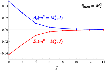
Figure 4: Values of $A_{s,u}$ and $B_{s,u}$, defined in Eq. (29), for the smearing functions Eq. (35). We have taken $m_{i}$ equal to its lowest value, $m_{i}=M_{s}\ (M_{u})$ in $A_{s},B_{s}$ ($A_{u},B_{u}$).

An example of smearing functions that satisfy all the requirements mentioned above are

$$A(t)=(1-\sqrt{-t/|t|_{\text{max}}})^{5}\quad\text{and}\quad B(t)=-0.885|t|_{\text{max}}(1-\sqrt{-t/|t|_{\text{max}}})^{5}\,.$$ (35)

We have checked explicitly that the functions above satisfy the inequalities Eq. (30) and Eq. (31) for general $m_{i}$ and $J_{i}$. For the lowest value $m_{i}=M_{s,u}$, we show $A_{s,u}$ and $B_{s,u}$ in Fig. 4 as a function of $J_{i}$. As we increase $J_{i}$ the values of $A_{s,u}$ and $B_{s,u}$ are difficult to get numerically, but we show in Appendix A that the conditions Eq. (30) and Eq. (31) can be satisfied for $J\to\infty$. In this limit the smeared functions decay like $1/J^{3}$, property which we derive analytically in Appendix A, but also observe in Fig. 4. The relations Eq. (30) and Eq. (31) are also satisfied when the masses of the states in the $s$ channel are smaller than $|t|_{\text{max}}$, i.e, for $M_{s}<M_{u}$.

We notice that the functions Eq. (35) also satisfy

$$A_{s,u}(m_{i},J_{i})\geq 0\,,$$ (36)

indicating that each term of Eq. (27) is positive. This shows that the sum rule Eq. (27) is exactly what we were looking for, an $O(1/m^{4})$ positive sum rule.

Plugging the smearing functions Eq. (35) into Eq. (32), we find the bound

$$\frac{M_{u}^{4}\kappa^{2}_{g}}{M_{P}^{2}F^{2}_{\pi}}+0.015\frac{\kappa_{3}^{2}M_{u}^{8}}{M_{P}^{4}}\lesssim 48\ln\bigg{(}\frac{M_{u}}{M_{\text{IR}}}\bigg{)}\,,$$ (37)

where $M_{\text{IR}}$ is an IR-cutoff that we are forced to introduce to regularize the logarithmically divergent integral $\int dt{A(-t)}/{t}$. This is a well-known fact of 4D gravity that also appears in constraints from time delay in the eikonal limit [31]. We must keep $M_{\text{IR}}$ as an independent parameter but we can assume to take values close to $M_{u}$ such that $\ln({M_{u}}/{M_{\text{IR}}})\sim O(1)$. Although the bound Eq. (37) could be improved by a better selection of smearing functions [22], we have checked that the result does not change substantially. Since both terms on the LHS of Eq. (37) are positive, we can derive the bound

$$\left|\frac{M_{u}^{2}\kappa_{g}}{M_{P}F_{\pi}}\right|\lesssim 7\ln^{\frac{1}{2}}\bigg{(}\frac{M_{u}}{M_{\text{IR}}}\bigg{)}\,.$$ (38)

We recall that $M_{u}$ in Eq. (38) corresponds to the mass of the lightest state of spin $4$ or higher. Therefore Eq. (38) can be interpreted as a bound due to the presence of the anomaly, $\kappa_{g}\not=0$, on the mass of states with $J\geq 4$ and nonzero coupling to two gravitons, $g_{+-,i}\not=0$. These states are of type $n=1,2$ as defined in Table 5. Similarly, a bound on $M_{u}$ can also be derived from Eq. (38) even when $\kappa_{g}=0$ as long as $\kappa_{3}\not=0$ (this is similar to the bound in [22]). Nevertheless, $\kappa_{3}\not=0$ is not necessarily guaranteed by any intrinsic UV condition of the model such as the anomaly.

There are other ways to bound $\kappa_{g}$ besides the one given above. An alternative possibility is shown in Appendix B where we obtain a bound on $\kappa_{g}$ from the Wilson coefficient $b_{0,0}$:

$$\frac{M_{u}\kappa_{g}^{2}}{M_{P}^{3}F_{\pi}^{2}}+0.023\frac{M_{u}^{5}\kappa_{3}^{2}}{M_{P}^{5}}\lesssim 21\sqrt{b_{0,0}}\ln^{\frac{1}{2}}\bigg{(}\frac{M_{u}}{M_{\text{IR}}}\bigg{)}\,.$$ (39)

6.2 Eta-graviton scattering

Similar bounds as the ones found above can be obtained from amplitudes involving external gravitons and pseudo-scalars $\eta$ shown in Fig. 2. As we will see below, the bound derived in these cases will be parametrically similar to Eq. (38).

Below we will derive the simplest bound from the elastic process $\eta h^{+}\rightarrow\eta h^{+}$ (B in Fig. 2), while in Appendix C we will also show how to construct a bound from the process $\eta h^{+}\rightarrow h^{+}h^{+}$ (C in Fig. 2) using a trigonometric inequality. The same logic could be also used to obtain bounds from $\eta h^{+}\rightarrow\eta\eta$ (D in Fig. 2), which however we will not discuss because they are similar to the ones derived here. We will show in Appendix C.1 how in these cases the eikonal limit can be recovered leading to a similar bound as the one derived in [22] for $\kappa_{3}$.

The amplitude for the process $\eta h^{+}\rightarrow\eta h^{+}$ at low energy is given by

$${\cal M}_{\eta+\eta-}\rightarrow s^{2}u^{2}\bigg{(}-\frac{1}{M_{P}^{2}stu}-\frac{\kappa_{g}^{2}t}{M_{P}^{4}F_{\pi}^{2}su}+...\bigg{)}\,.$$ (40)

At fixed $t$, we use the dispersion relation $\oint_{C_{\infty}}M_{\eta+\eta-}/s^{2}u=0$ instead of $\oint_{C_{\infty}}M_{\eta+\eta-}/s^{3}=0$ (both integrants have the same high-energy behaviour) to avoid the appearance of Wilson coefficients. We find

$$\frac{-1}{M_{P}^{2}t}-\frac{\kappa_{g}^{2}t}{M_{P}^{4}F_{\pi}^{2}}=\Big{\langle}\frac{d_{-2,-2}^{J}(1+2t/m^{2})}{m^{2}(m^{2}+t)}\Big{\rangle}^{g_{\eta+}^{2}}+\Big{\langle}\frac{d_{2,2}^{J}(1+2t/m^{2})}{(m^{2}+t)^{2}}\Big{\rangle}^{g_{\eta-}^{2}}\,.$$ (41)

Since ${\cal M}_{\eta+\eta-}$ is $s\leftrightarrow u$ symmetric, we have $M_{u}=M_{s}$. Integrating Eq. (41) in $t$ with a smearing function $C(t)$, we get

$$\int^{0}_{-|t|_{\text{max}}}C(t)\bigg{(}\frac{-1}{M_{P}^{2}t}-\frac{\kappa_{g}^{2}t}{M_{P}^{4}F_{\pi}^{2}}\bigg{)}dt=\bigg{(}\sum_{i}C_{s}(m_{i},J_{i})g_{\eta+,i}^{2}+\sum_{j}C_{u}(m_{j},J_{j})g^{2}_{\eta-,j}\bigg{)}\,,$$ (42)

where we defined the functions

$$C_{s}(m,J) = \int_{-|t|_{\text{max}}}^{0}C(t)\frac{d_{-2,-2}^{J}(1+2t/m^{2})}{m^{2}(m^{2}+t)}\ dt\,,$$

$$C_{u}(m,J) = \int_{-|t|_{\text{max}}}^{0}C(t)\frac{d_{2,2}^{J}(1+2t/m^{2})}{(m^{2}+t)^{2}}\ dt\,.$$ (43)

Demanding that the smearing function $C(t)$ satisfies

$$C_{s,u}(m,J)\geq 0\hskip 42.67912pt\forall m^{2}\geq M_{s}^{2}=M_{u}^{2}\ ,\ \forall J\geq 2\,,$$ (44)

we can use Eq. (42) to obtain

$$\int_{0}^{|t|_{\text{max}}}C(-t)\bigg{(}\frac{1}{M_{P}^{2}t}+\frac{\kappa_{g}^{2}t}{M_{P}^{4}F_{\pi}^{2}}\bigg{)}dt\geq 0\,.$$ (45)

To find a non-trivial bound on $\kappa_{g}^{2}$ from the equation above we need the first and second term to have opposite signs. A smearing function that satisfies these conditions and also guarantees the positivity requirement Eq. (45) is

$$C(t)=J_{0}(\sqrt{-\beta^{2}t/|t|_{\text{max}}})\left(1-\sqrt{-t/|t|_{\text{max}}}\right)^{3}\ \ \ (\beta\geq 5)\,,$$ (46)

where $J_{0}$ is the zero-order Bessel function. To maximize the bound we take

$$|t|_{\text{max}}=M_{s}^{2}=M_{u}^{2}\equiv M_{2}^{2}\,,$$ (47)

where $M_{2}$ corresponds to the mass of the lightest $J\geq 2$ state with $g_{\eta\pm,i}\not=0$. These states are of type $n=1,2,3$ as defined in Table 5. Using Eq. (47) in Eq. (46) and setting $\beta\sim 7.2$ (this value maximizes the bound), Eq. (45) yields

$$\frac{M_{2}^{2}\kappa_{g}}{M_{P}F_{\pi}}\lesssim 30\ln^{\frac{1}{2}}\bigg{(}\frac{M_{2}}{M_{\text{IR}}}\bigg{)}\,.$$ (48)

Bounds can also be derived from inelastic processes. In Appendix C we use the process $\eta h^{+}\rightarrow h^{+}h^{+}$ to obtain the bound

$$\left|\frac{M_{2}^{2}\kappa_{g}}{M_{P}F_{\pi}}-0.017\frac{M_{2}^{6}\kappa_{3}\kappa_{g}}{M_{P}^{3}F_{\pi}}\right|\lesssim 106\ln\bigg{(}\frac{M_{2}}{M_{\text{IR}}}\bigg{)}\,.$$ (49)

The second term on the LHS, which can have either sign, seems to allow $\kappa_{g}$ to be unbounded. Nevertheless, the numerical coefficient in front of this second term could have been made much smaller by a better selection of the smearing function. In fact, as discussed in Appendix C.1, it goes to zero in the eikonal limit.

7 Phenomenological Implications

The bounds Eq. (38) and Eq. (48) can be interpreted as an upper bound for $M_{u}$ and $M_{2}$ respectively in theories with $\kappa_{g}\not=0$. Since both bounds are almost identical, we will only consider here the implications for the upper bound on $M_{u}$.

This upper bound represents the mass scale at or below which $J\geq 4$ states must appear in ${\cal L}_{\rm EFT}(\eta,h)$, the EFT of $\eta$ and gravitons. This mass scale, which from now on we will refer to as $\Lambda_{\text{caus}}$, represents then a cutoff scale for ${\cal L}_{\rm EFT}(\eta,h)$. Taking $M_{\rm IR}=O(M_{u})$ in Eq. (38), we find that this is parametrically given by

$$\Lambda_{\text{caus}}\sim\sqrt{\frac{M_{P}F_{\pi}}{\kappa_{g}}}\,.$$ (50)

For $\kappa_{g}\sim 1$, $\Lambda_{\text{caus}}$ lies around the geometric mean of $M_{P}$ and $F_{\pi}$.

The cutoff scale $\Lambda_{\text{caus}}$ is smaller than $\Lambda_{\text{pert}}$, the naive perturbative cutoff scale of ${\cal L}_{\rm EFT}(\eta,h)$ defined as the scale at which loops become of order tree-level. For ordinary gravity, $\Lambda_{\text{pert}}$ is around $M_{P}$, but for ${\cal L}_{\rm EFT}(\eta,h)$ with the coupling Eq. (2), this is given by

$$\Lambda_{\text{pert}}\sim\sqrt[3]{\frac{M_{P}^{2}F_{\pi}}{\kappa_{g}}}\,.$$ (51)

For $F_{\pi}\lesssim\kappa_{g}M_{P}$, we have indeed that $\Lambda_{\text{caus}}\lesssim\Lambda_{\text{pert}}$.

7.1 Models of axions

Axions arise as pseudo-scalar Goldstone bosons of non-linearly realized global $U(1)$ symmetries. In the case of the QCD axion, the $U(1)$ has a $U(1)-SU(3)_{c}-SU(3)_{c}$ anomaly that induces the interaction term ${\cal L}_{\rm int}=aG\tilde{G}/f_{a}$, being $G$ the $SU(3)_{c}$ field-strength and $f_{a}$ the axion decay constant. It is natural to expect that these models also have a $U(1)$-gravitational anomaly (as is the case in most proposed models), leading to the presence of Eq. (2) with $\eta$ identified as the axion $a$ and $F_{\pi}/\kappa_{g}\sim f_{a}$. In this case, Eq. (50) tells us that the EFT of axions cannot be extrapolated beyond

$$\Lambda_{\text{caus}}\sim\sqrt{M_{P}f_{a}}\,,$$ (52)

where new states must appear. This cutoff, expected to be present in any axion-like EFT, is smaller than any other cutoff scale based on perturbativity such as Eq. (51).

In explicit weakly-coupled UV realizations of axion models, new physics indeed appears below Eq. (52). For instance, in axion models in which $\kappa_{g}$ is one-loop generated by massive extra quarks, the mass of these states is always below Eq. (52).

7.2 Models of massive higher-spin resonances

Let us now consider the class of models consisting of an infinite set of states $R_{i}$ with arbitrary spin $J$ and a characteristic coupling $g_{*}$. We will be considering the weak-coupling limit $g_{*}\to 0$. More realistic scenarios containing different sets of states, each with its own distinct $g_{*}$, will be introduced later.

We couple this class of models to gravity. We can schematically write the Lagrangian of the states $R_{i}$ interacting with gravity as

$${\cal L}=M_{P}^{2}{\cal R}+\frac{1}{g^{2}_{*}}\left[(\partial R_{i})^{2}+m^{2}_{i}R^{2}_{i}+m_{i}R_{i}^{3}+h_{\mu\nu}T^{\mu\nu}(R_{i})+\cdots\right]\,,$$ (53)

where ${\cal R}$ is the Ricci scalar that contains the kinetic term of the graviton and $T^{\mu\nu}(R_{i})$ is the energy-momentum tensor that can be expanded as a polynomial in $R_{i}$. Assuming that the interactions of $\eta$ have the same parametric dependence as those of $R_{i}$ given in Eq. (53), we can estimate

$$F^{2}_{\pi}\sim M^{2}/g^{2}_{*}\ ,\ \ \ \kappa_{g}\sim 1/g^{2}_{*}\,,$$ (54)

where $M$ is the mass of the lightest resonance, in principle, not necessarily a $J\geq 2$ state.

One could guess that in the formal limit $g_{*}\to 0$ and $M_{P}/M\to\infty$, the model is valid at all energies. Nevertheless, this is not true. From the interchange of resonances as in Fig. 5, the graviton 2-point function $\Pi(q)=q^{2}$ (stripping off the polarization tensor) receives corrections that, on dimensional grounds, can be estimated to be

$$\Delta\Pi(q)\sim\frac{q^{4}}{g^{2}_{*}M_{P}^{2}}\,.$$ (55)

These corrections can overcome the tree-level contribution for momentum $q$ above the scale

$$g_{*}M_{P}\equiv\Lambda_{\rm QG}\,,$$ (56)

that therefore corresponds to a UV cutoff scale in the theory. Although we determined the cutoff scale $\Lambda_{\rm QG}$ from naive perturbativity, it has been recently argued that this cutoff scale is rigorous and related with UV completions of gravity [41]. Therefore, we expect at $\Lambda_{\rm QG}$ states associated to quantum gravity, such as string modes, which are unrelated to the states in our model of resonances.

We will work in the limit

$$M_{P}\to\infty\ ,\ \ \ g_{*}\to 0\ ,\ \ \ \Lambda_{\rm QG}={\rm Fixed}\,.$$ (57)

In this limit, the bound based on causality Eq. (50) goes as

$$\Lambda_{\text{caus}}\sim\sqrt{g_{*}M_{P}M}\,,$$ (58)

that using Eq. (56) can be written as

$$\Lambda_{\text{caus}}\sim\sqrt{\Lambda_{\text{QG}}M}\,.$$ (59)

Since $\Lambda_{\text{QG}}\gg M$, the scale where spin$\geq 4$ states must appear is always smaller than the scale of quantum gravity. This is therefore an important bound for these type of models when $\kappa_{g}\not=0$.

Figure 5: Contribution to the graviton propagator due to the exchange of resonances.

7.2.1 Strongly-coupled large-$N_{c}$ gauge theories

Models with similar properties as the ones described above are strongly-coupled gauge theories with $N_{F}$ fermions ($f_{L,R}$) in the $N_{c}\to\infty$ limit. In this section we will consider that the ’tHooft coupling, $g^{2}_{\rm YM}N_{c}$, is not large, and then physical quantities are characterized only by $N_{c}$ and $M$, the mass gap of the theory [42, 43].

The pseudo-scalar $\eta$ can appear in these theories as the Goldstone boson associated to the chiral breaking $U(1)_{L}\times U(1)_{R}\to U(1)_{V}$. In principle, since the axial $U(1)_{A}$ current $J^{\mu}_{A}=\sum_{f}\bar{f}\gamma^{\mu}\gamma^{5}f$ is not conserved at the quantum level due to the axial anomaly, $\eta$ gets a mass of order $m^{2}_{\eta}\sim N_{F}M^{4}/F_{\pi}^{2}$ [44, 45]. In the large-$N_{c}$ limit, however, $m^{2}_{\eta}\to 0$ since $F^{2}_{\pi}\sim N_{c}M^{2}\to\infty$. Unlike the models described above, large-$N_{c}$ gauge theories contain two distinct sets of resonances, mesons and glueballs, whose 3-point couplings scale differently at large $N_{c}$:

$$g_{\rm meson}\sim\frac{1}{\sqrt{N_{c}}}\ ,\ \ \ \ g_{\rm glueball}\sim\frac{1}{N_{c}}\,.$$ (60)

By switching on the gravitational interactions, the coupling Eq. (2) is generated due to the $U(1)$-gravitational anomaly, with $\kappa_{g}\sim N_{c}\sqrt{N_{F}}$. For the particular case of $SU(N_{c})$ gauge theories, we have

$$\kappa_{g}=\frac{N_{c}\sqrt{N_{F}}}{192\pi^{2}}\,.$$ (61)

Corrections to the graviton propagator from Fig. 5 are dominated by glueballs, leading at $q\gg M$ to

$$\Delta\Pi(q)\sim\frac{N_{c}^{2}q^{4}}{M_{P}^{2}}\ln q\,.$$ (62)

This correction can also be understood as arising at high energy from a loop of gluons. Therefore we can define

$$\Lambda_{\rm QG}=\frac{M_{P}}{N_{c}}\,,$$ (63)

as the scale where the corrections dominate over tree-level. Using these relations in Eq. (50), we get

$$\Lambda_{\text{caus}}\sim\sqrt{\Lambda_{\text{QG}}M\sqrt{\frac{N_{c}}{N_{F}}}}\,,$$ (64)

that tells us that in the strict $N_{c}\to\infty$ limit at $N_{F}$ fixed, $\Lambda_{\text{caus}}$ overcomes $\Lambda_{\text{QG}}$ and no limit can be deduced for the $J\geq 4$ resonances of the gauge sector.

Notice however that this is not the case for theories in the Veneziano limit, $N_{c}\to\infty$ with $N_{c}/N_{F}$ fixed. In this case the bound Eq. (64) remains finite, predicting that $J\geq 4$ resonances must be present below $\Lambda_{\text{QG}}$.

Let us also point out that in the presence of glueballs, we could also expect $\kappa_{3}\sim N^{2}_{c}/M^{2}$. Therefore we can use Eq. (37) to obtain

$$\Lambda_{\rm caus}\sim\sqrt{\frac{M_{P}}{\kappa_{3}^{1/2}}}\sim\sqrt{\Lambda_{\rm QG}M}\,,$$ (65)

implying that, contrary to Eq. (64), the bound on the mass of $J\geq 4$ states lies below $\Lambda_{\rm QG}$ even for $N_{c}\to\infty$. Nevertheless, this results applies only if $\kappa_{3}\not=0$ that is not guaranteed by any UV anomaly.

7.2.2 Holographic AdS₅ models

Another class of models with similar properties are holographic theories based on the AdS/CFT correspondence. These are weakly-coupled models in more than 4D conjectured to be the duals of strongly-coupled models in the large-$N_{c}$ limit. The most famous example is the 10D AdS${}_{5}\times S^{5}$ model dual to ${\cal N}=4$ supersymmetric Yang-Mills theories [46]. In the large ’tHooft coupling limit, $\lambda\equiv g_{\rm YM}^{2}N_{c}\to\infty$, the $J>2$ states (associated to string states) of the dual 10D theory become infinitely heavy, and the light spectrum consists of states of $J=0,1,2$. It is then interesting to understand whether the cutoff $\Lambda_{\rm caus}$ derived above imposes constraints on this class of models.

We will consider here a simple 5D model that at low-energies consists of a 4D massless $\eta$ and a graviton. The 5D Lagrangian is given by (up to marginal operators)

$${\cal L}_{5}=\int d^{5}x\sqrt{-g}\left[M_{P5}^{3}{\cal R}+M_{5}F_{MN}^{2}+\kappa_{5}\,\epsilon_{MNPQR}A^{M}{\cal R}^{NPA}_{B}{\cal R}^{QRB}_{A}\right]\,,$$ (66)

where $F_{MN}$, ${\cal R}$ and ${\cal R}^{MNPQ}$ are respectively the gauge field-strength, Ricci scalar and Riemann tensor; $M_{P5}$ and $1/M_{5}$ are respectively the 5-dimensional Planck scale and gauge-coupling squared, and $\kappa_{5}$ is the dimensionless coefficient of the Chern-Simons term related with the chiral-gravitational anomaly.

We assume the metric is AdS₅, $ds^{2}=(L/z)^{2}(\eta_{\mu\nu}dx^{\mu}dx^{\nu}-dz^{2})$, being $L$ the AdS curvature radius and $z$ the 5th dimension. We also consider that the extra dimension is compactified by placing two boundaries, one at $z=1/\Lambda_{\rm UV}$ (UV-boundary) and another at $z=1/\Lambda_{\rm IR}$ (IR-boundary) with $\Lambda_{\rm UV}\gg\Lambda_{\rm IR}$. The model is then defined on the line segment $1/\Lambda_{\rm UV}\leq z\leq 1/\Lambda_{\rm IR}$. This set-up is referred as a Randall-Sundrum model [47].

As boundary conditions we choose $A_{\mu}=0$ at both boundaries such that at low-energy only the fifth-component of the gauge boson $A_{5}$ (a pseudo-scalar) remains in the spectrum. At low-energy $E\ll\Lambda_{\rm IR}$ then the model has two massless states, $A_{5}$ to be identified with $\eta$ and the zero-mode of the graviton $h_{\mu\nu}$. It is easy to check that the Chern-Simons term leads to Eq. (2) with $\kappa_{g}\propto\kappa_{5}$.

The model contains an infinite set of massive resonances corresponding to the Kaluza-Klein (KK) modes of the graviton and gauge boson with masses $\sim r\Lambda_{\rm IR}$ where $r\in\mathbb{N}^{+}$. Notice that the model only contains $J=1,2$ KK states. Their 3-point coupling squared for KK graviton and gauge bosons are parametrically given by

$$g^{2}_{\rm KK,grav}\sim 1/(M_{P5}L)^{3}\ ,\ \ \ \ g^{2}_{\rm KK,gauge}\sim 1/(M_{5}L)\,.$$ (67)

Therefore by working in the limit

$$(M_{P5}L)^{3}\to\infty\ ,\ \ \ M_{5}L\to\infty\,,$$ (68)

the couplings of the model go to zero becoming a free theory. It is easy to calculate $F_{\pi}$, $M_{P}$ and $\kappa_{g}$ for the EFT of the 4D massless modes. One gets

$$F_{\pi}^{2}=M_{5}L\Lambda_{\rm IR}^{2}\ ,\ \ \ \ M_{P}^{2}=(M_{P5}L)^{3}\Lambda_{\rm UV}^{2}\ ,\ \ \ \ \kappa_{g}=\kappa_{5}\,.$$ (69)

In the limit Eq. (68), the only UV cutoff of the model is given by $\Lambda_{\rm UV}$. Indeed, this scale can be identified with $\Lambda_{\rm QG}$ by looking again to the corrections of the graviton propagator [48]:

$$\Delta\Pi(q)=\frac{(M_{P5}L)^{3}}{M_{P}^{2}}q^{4}\ln q=\frac{1}{\Lambda_{\rm UV}^{2}}q^{4}\ln q\,,$$ (70)

that becomes larger than the tree-level contribution above $\Lambda_{\rm QG}\sim\Lambda_{\rm UV}$.

Plugging Eq. (69) into Eq. (50), we obtain that this theory becomes acausal at energies above

$$\Lambda_{\rm caus}\sim r_{5}\sqrt{\Lambda_{\rm UV}\Lambda_{\rm IR}}\ ,\ \ \ \ \ r_{5}\equiv\left(\frac{M_{P5}^{3}M_{5}L^{4}}{\kappa_{5}^{2}}\right)^{1/4}\,.$$ (71)

If we demand this scale to be bigger than $\Lambda_{\rm UV}$, in order to avoid problems with causality below the UV cutoff, we obtain the bound

$$\Lambda_{\rm caus}\gtrsim\Lambda_{\rm UV}\ \ \longrightarrow\ \ r_{5}\gtrsim\sqrt{\frac{\Lambda_{\rm UV}}{\Lambda_{\rm IR}}}\,,$$ (72)

that using Eq. (67) can be rewritten as

$$\kappa_{5}\,g_{\rm KK,grav}\,g_{\rm KK,gauge}\lesssim\frac{\Lambda_{\rm IR}}{\Lambda_{\rm UV}}\ll 1\,.$$ (73)

This result looks quite surprising from the point of view of the 5D theory. It tells us that either we have problems with causality ($\Lambda_{\rm caus}\lesssim\Lambda_{\rm UV}$) or the couplings of the KK spin-1 and spin-2 states are not free parameters but related by Eq. (73). Interestingly, Eq. (72) can be satisfied when the 5D parameters are matched with the ones expected from the dual description:

$$(M_{P5}L)^{3}\sim N_{c}^{2}\ ,\ \ \ M_{5}L\sim N_{c}\ ,\ \ \ \kappa_{5}\sim N_{c}\,,$$ (74)

that leads to $r_{5}\sim N_{c}^{1/4}\to\infty$ in the large-$N_{c}$ limit.

7.2.3 5D models in a compact flat space

Similarly, a model of weakly-coupled resonances can be obtained from the 5D model of Eq. (66) in flat space with the extra dimension compactified in a segment of length $L$. We get in this case [49]

$$F^{2}_{\pi}\sim M_{5}/L\ ,\ \ M_{P}^{2}\sim M^{3}_{P5}L\,,$$ (75)

and from Eq. (50)

$$\Lambda^{4}_{\rm caus}\sim\frac{M_{5}M^{3}_{P5}}{\kappa_{5}^{2}}\,.$$ (76)

Note that since $\Lambda_{\rm caus}$ in Eq. (76) does not depend on $L$, this should be a causality cutoff for any 5D model defined by Eq. (66), independently of the spacetime metric. In fact, we could have derived this bound directly in 5D rather than in 4D.

We can again ask what conditions the 5D parameters must satisfy in order to have $\Lambda_{\rm caus}$ above the cutoff scale of the 5D theory that, based on naive perturbativity, is given by $\Lambda_{5}\sim{\rm Min}[M_{5},M_{P5}]$. We see that (taking for concreteness $M_{P5}<M_{5}$)

$$\Lambda_{\rm caus}\gtrsim\Lambda_{5}\ \ \longrightarrow\ \ |\kappa_{5}|\lesssim\left(\frac{M_{5}}{M_{P5}}\right)^{3/2}\,.$$ (77)

Surprisingly, this bound is not consistent with the scaling Eq. (74) in the large-$N_{c}$ limit. This implies that either new physics (states with $J\geq 4$) appears below the cutoff $\Lambda_{5}$, or the 5D parameters must depart from the simple scaling Eq. (74) to satisfy Eq. (77).

It is interesting to check what happens in explicit holographic models derived from string theory. Let us consider the model of [50], based on a $D3/D7$ system. One has

$$M^{3}_{P5}\propto N_{c}^{2}\ ,\ \ M_{5}\propto N_{c}\ ,\ \ \kappa_{5}\propto N_{c}\ ,\ \ M_{\rm string}\propto\lambda^{1/4}\,,$$ (78)

where $M_{\rm string}$ is the string scale. Using Eq. (78) in Eq. (76), one finds

$$\Lambda_{\rm caus}\propto N_{c}^{1/4}\,.$$ (79)

Consequently, for small string coupling $g_{\rm string}=g^{2}_{\rm YM}/4\pi\lesssim 1$, where $\lambda\lesssim N_{c}$, this model predicts that $M_{\rm string}\lesssim\Lambda_{\rm caus}$, i.e., states with $J\geq 4$ indeed appear below the causality bound.

8 Conclusions

We have studied the implications of causality and unitarity on theories with a pseudo-Goldstone $\eta$ coupled to two gravitons like in Eq. (2), an interaction that arises from $U(1)$-gravitational anomalies. We first considered gravity as an external source probing the theories, and showed that no constraint can be obtained in this case on the anomaly coefficient $\kappa_{g}$.

Therefore, we needed to couple the theory to dynamical gravitons, and consider dispersion relations with $1/t$ poles arising from the graviton exchange. Integrating these dispersion relations over $t$ weighted by some particular functions to guarantee positivity, we have been able to derived bounds on $\kappa_{g}$. In particular, from the graviton-graviton scattering amplitude, we have derived Eq. (38), that can be interpreted as an upper bound on the mass of $J\geq 4$ states. Similarly, from the eta-graviton scattering amplitude, we obtained the bound Eq. (48) that provided an upper bound on the mass of $J\geq 2$ states.

These upper bounds on the mass scale at which new states must appear can be considered as a cutoff scale for the EFT of $\eta$ and the graviton. For axion EFTs we have seen that we expect this cutoff to be at $\Lambda_{\rm caus}\sim\sqrt{M_{P}f_{a}}$.

For strongly-coupled gauge theories in the large-$N_{c}$ limit, that can be described as models of massive higher-spin resonances, the cutoff scale $\Lambda_{\rm caus}$ was found to be larger than the quantum gravity scale due to the presence of glueballs whose couplings scale differently from that of mesons, as shown in Eq. (60). This happens if the number of fermions is much smaller than $N_{c}$ and the ’tHooft coupling $g_{\rm YM}^{2}N_{c}$ is not large. For large ’tHooft coupling, however, where these theories can have an holographic 5D dual, we have seen that $\Lambda_{\rm caus}$ can lie below any other cutoff scale (based on perturbativity), leading to consistency conditions on the parameters of the 5D models, as for example Eq. (73) and Eq. (77).

Our analysis for 4D theories with $U(1)$-gravitational anomalies deserves future research. For example, one could try to improve the bounds by a better choice of the smearing functions, explore UV completions beyond tree-level, or extend the analysis to theories in higher dimensions. We leave all this for future work.

Acknowledgments

We are very grateful to Francesco Riva and Brando Bellazzini for valuable discussions. We also thank Francesco Riva for a critical reading of the manuscript. This work has been partly supported by the research grants 2021-SGR-00649 and PID2023-146686NB-C31 funded by MICIU/AEI/10.13039/501100011033/ and by FEDER, UE. T.M is partly supported by the Yan-Gui Talent Introduction Program (grant No. 118900M128) and Chinese Academy of Sciences Pioneer Initiative ”Talent Introduction Plan”.

Appendix A Positivity in smeared dispersion relation at large $J$

Here we show which conditions the smearing functions must satisfy in order to guarantee positivity conditions as Eq. (36) in the limit $J\to\infty$. In particular, we will study the smeared Wigner $d$-function appearing in Eq. (29) that we generically write as (changing variables $t\to-t$)

$$F(m,J)=\int_{0}^{|t|_{\text{max}}}f(t)\,d_{h,h}^{J}(1-2t/m^{2})dt\,.$$ (80)

Here $f(t)$ refers either to the smearing function, $A(-t)$ or $B(-t)$, or the quotient $A(t)/(m^{2}-t)^{3}$ or $B(t)/(m^{2}-t)^{4}$ appearing in Eq. (29).

In the limit $J\to\infty$ the Wigner $d$-functions have a well-known behaviour given by the Darboux formula

$$d_{h,h}^{J}(1-2t/m^{2})\underset{J\rightarrow\infty}{\longrightarrow}\sqrt{\frac{m^{2}}{\pi J\sqrt{(m^{2}-t)t}}}\cos\Big{(}2(J+1/2)\sin^{-1}(\sqrt{t/m^{2}})-\pi/4\Big{)}\,,$$ (81)

which in turn we can expand in the regimes $t/m^{2}\to 0$ and $t/m^{2}\to 1$, giving

$$d_{h,h}^{J}(1-2t/m^{2})\underset{J\rightarrow\infty}{\longrightarrow}\begin{cases}J_{0}\big{(}2\sqrt{\mathcal{J}^{2}t/m^{2}}\big{)}+O({J}^{-3/2})\hskip 110.96556ptt/m^{2}\to 0\,,\\[12.0pt] (-1)^{h+J}J_{2h}\big{(}2\sqrt{\mathcal{J}^{2}(1-t/m^{2})}\big{)}+O({J}^{-3/2})\hskip 34.14322ptt/m^{2}\to 1\,,\end{cases}$$ (82)

where we defined $\mathcal{J}^{2}=J(J+1)$. Note that the limits above are correct as long as $t/m^{2}$ goes to zero (or $1$) slower than $1/J$, otherwise the expansion in $t/m^{2}$ and the one in $J$ do not commute (first term in $J$ becomes of the same order as the second and so on). With these limits in mind we can go back to the smeared dispersion relation Eq. (80).

Let us initially consider the case where $m^{2}=|t|_{\text{max}}=M^{2}$. We can divide the integration region in three parts and change coordinates $t=p^{2}$:

$$F(M,J)=\bigg{(}\int_{0}^{a}+\int_{a}^{M-b}+\int_{M-b}^{M}\bigg{)}f(p)d_{h,h}^{J}(1-2p^{2}/M^{2})pdp\,,$$ (83)

We choose $a,b$ to be zeros of the Wigner $d$-functions. This assures that if $f(p)$ is a regular function, the middle integral in Eq. (83) goes to zero in the large $J$ limit. This happens because we convolute the rapidly oscillating Wigner $d$-function with a regular function, such that the integral averages out to zero. We are left then with the integration regions between $(0,a)$ and $(M-b,M)$. By taking $a$ and $b$ small, we can use Eq. (82) and analytically perform the first and third integration in Eq. (83) after Taylor expanding $f(p)$ for $p$ close to zero and $M$ respectively. We find

$$F(M,J)\underset{J\rightarrow\infty}{\longrightarrow}\bigg{(}f^{\prime}(0)\frac{1}{8J^{3}}+O(J^{-4})\bigg{)}+(-1)^{h+J}\bigg{(}f(M)\frac{h}{2J^{2}}+O(J^{-4})\bigg{)}\,.$$ (84)

By demanding $f(M)=0$, we assure that the oscillating term in $J$ becomes $O(1/J^{4})$ and is subdominant compared to the non-oscillating term, as long as $f^{\prime}(0)\not=0$. We then get $F(M,J)\to\ f^{\prime}(0)/J^{3}$ at large $J$. This behaviour is also observed in our numerical results shown in Fig. 4.

We conclude then that at large $J$ and for $m=M$, positivity is guaranteed if $f(M)=0$ and $f^{\prime}(0)>0$. These conditions determined our smearing functions in Eq. (35) and Eq. (46).

For the case $m^{2}>|t|_{\text{max}}$, one can repeat the same procedure as above, with the exception that we cannot use the expansion Eq. (82) for $t/m^{2}\to 1$. One gets again that $F(m,J)$ drops at large $J$ as $\sim 1/J^{3}$ with definite sign.

Appendix B Alternative bound on $\kappa_{g}$ from graviton scattering

An alternative bound to Eq. (38) can be derived in the following way. Let us consider the smeared dispersion relation Eq. (27) and Eq. (28) and define

$$\hat{A}_{s,u}(m_{i},J_{i})\equiv A_{s,u}(m_{i},J_{i})\,m_{i}^{4}\ \ \ {\rm and}\ \ \ \hat{B}_{s,u}(m_{i},J_{i})\equiv B_{s,u}(m_{i},J_{i})\,m_{i}^{6}\,.$$ (85)

Using the trigonometric (Cauchy-Schwartz) inequality

$$\big{(}\sum_{i}a_{i}b_{i}\big{)}^{2}\leq\big{(}\sum_{i}a_{i}a_{i}\big{)}\big{(}\sum_{i}b_{i}b_{i}\big{)}\,,$$ (86)

we can write

$$\bigg{(}\sum_{i}\frac{\hat{B}_{s}(m_{i},J_{i})}{m_{i}^{6}}g_{++,i}^{2}+\sum_{j}\frac{\hat{B}_{u}(m_{j},J_{j})}{m_{j}^{6}}g^{2}_{+-,j}\bigg{)}^{2}\leq\hskip 113.81102pt$$

$$\bigg{(}\sum_{i}\frac{(\hat{B}_{s}(m_{i},J_{i}))^{2}}{m_{i}^{4}}g_{++,i}^{2}+\sum_{j}\frac{(\hat{B}_{u}(m_{j},J_{j}))^{2}}{m_{i}^{4}}g_{+-,j}^{2}\bigg{)}\bigg{(}\sum_{i}\frac{g_{++,i}^{2}}{m_{i}^{8}}+\sum_{j}\frac{g_{+-,j}^{2}}{m_{i}^{8}}\bigg{)}\,.$$ (87)

The two terms on the RHS can be related to other physical quantities as follows. First, demanding to the smearing functions to satisfy

$$(\hat{B}_{s}(m,J))^{2}\leq\hat{A}_{s}(m,J)\ \ \text{and}\ \ (\hat{B}_{u}(m,J))^{2}\leq\hat{A}_{u}(m,J)\,,$$ (88)

we have

$$\bigg{(}\sum_{i}\frac{\hat{B}_{s}(m_{i},J_{i})^{2}}{m_{i}^{4}}g_{++,i}^{2}+\sum_{j}\frac{\hat{B}_{u}(m_{j},J_{j})^{2}}{m_{i}^{4}}g_{+-,j}^{2}\bigg{)}\leq\bigg{(}\sum_{i}\frac{\hat{A}_{s}(m_{i},J_{i})}{m_{i}^{4}}g_{++,i}^{2}+\sum_{j}\frac{\hat{A}_{u}(m_{j},J_{j})}{m_{i}^{4}}g_{+-,j}^{2}\bigg{)}\,,$$ (89)

where the RHS can be identified with the RHS of Eq. (27). Secondly, using Eq. (26) for $t\rightarrow 0$, we obtain

$$b_{0,0}=\sum_{i}\frac{g_{++,i}^{2}}{m_{i}^{8}}+\sum_{j}\frac{g_{+-,j}^{2}}{m_{i}^{8}}\,.$$ (90)

Now, using Eq. (89) and Eq. (90) together with Eq. (27) and Eq. (28), we can rewrite Eq. (87) as

$$\bigg{(}\int_{0}^{|t|_{\text{max}}}dt\bigg{(}\frac{\kappa_{g}^{2}}{M_{P}^{4}F_{\pi}^{2}}+\frac{\kappa_{3}^{2}}{M_{P}^{6}}t^{2}\bigg{)}B(-t)\bigg{)}^{2}\leq\frac{b_{0,0}}{M_{P}^{2}}\int_{0}^{|t|_{\text{max}}}dt\frac{A(-t)}{t}\,.$$ (91)

Two functions $A(t)$ and $B(t)$ that guarantee Eq. (88) to be satisfied are

$$A(t)=B(t)=\frac{1}{|t|_{\text{max}}}\left(1-\sqrt{-{t}/{|t|_{\text{max}}}}\right)^{4}\,.$$ (92)

Plugging the above functions into Eq. (91) and taking $|t|_{\text{max}}=M^{2}_{u}$, we obtain the bound Eq. (39).

Appendix C Bounds from $\eta h^{+}\rightarrow h^{+}h^{+}$ and the eikonal limit

We can also use the process $\eta h^{+}\to h^{+}h^{+}$ to obtain a bound on $\kappa_{g}$. At low-energy the amplitude for this process is given by

$${\cal M}_{\eta+--}\to s^{3}tu\bigg{(}\frac{\kappa_{g}}{M_{P}^{3}F_{\pi}}\frac{1}{stu}+\frac{\kappa_{3}\kappa_{g}}{M_{P}^{5}F_{\pi}s}+e_{0,0}+\dots\bigg{)}\,,$$ (93)

where the first term comes from the graviton exchange and $e_{0,0},...$ are Wilson coefficients. From the $k=2$ dispersion relation in the complex $s$-plane at fixed $t$, one obtains a sum rule for $\kappa_{g}$:

$$\frac{\kappa_{g}}{M_{P}^{3}F_{\pi}}-\frac{\kappa_{3}\kappa_{g}}{M_{P}^{5}F_{\pi}}t^{2}=\bigg{\langle}\frac{d_{-2,0}^{J}(1+2t/m^{2})}{m^{4}}\bigg{\rangle}^{g_{\eta+}g_{--}}+\bigg{\langle}\frac{m^{2}d_{2,4}^{J}(1+2t/m^{2})}{(m^{2}+t)^{3}}\bigg{\rangle}^{g_{\eta-}g_{-+}}\,,$$ (94)

where, as in Eq. (24), we must be aware that the $t$-expansion is not convergent. Indeed, expanding in $t$ one finds that the LHS is $O(t^{0})$ while the RHS is $O(t)$. We therefore need to smear this sum rule. Using $D(t)$ as a smearing function we have

$$\int_{-|t|_{\text{max}}}^{0}dt\ D(t)\bigg{(}\frac{\kappa_{g}}{M_{P}^{3}F_{\pi}}-\frac{\kappa_{3}\kappa_{g}}{M_{P}^{5}F_{\pi}}t^{2}\bigg{)}=\sum_{i}D_{s}(m_{i},J_{i})g_{\eta+,i}g_{--,i}+\sum_{j}D_{u}(m_{j},J_{j})g_{\eta-,j}g_{-+,j}\,,$$ (95)

where

$$D_{s}(m,J) = \int_{-|t|_{\text{max}}}^{0}D(t)\ \frac{d_{-2,0}^{J}(1+2t/m^{2})}{(m^{2})^{2}}\ dt\,,$$

$$D_{u}(m,J) = \int_{-|t|_{\text{max}}}^{0}D(t)\frac{m^{2}d_{2,4}^{J}(1+2t/m^{2})}{(m^{2}+t)^{3}}\ dt\,.$$ (96)

Eq. (95) relates the anomaly coefficient $\kappa_{g}$ to sums involving products of different meson couplings that can have either sign. Therefore, as in Appendix B, we will need to use the trigonometric inequality Eq. (86) to relate the RHS of Eq. (95) to the elastic process $\cal M_{--++}$ (A2 in Fig. 1) and $\cal M_{\eta+\eta-}$ (B in Fig. 2) whose dispersion relations were already detailed in Sec. 6.1 and Sec. 6.2 respectively.

Using the trigonometric inequality Eq. (86), we have

$$\bigg{(}\sum_{i}\sqrt{C_{s}(m_{i},J_{i})}\sqrt{A_{s}(m_{i},J_{i})}g_{\eta+,i}g_{--,i}+\sum_{j}\sqrt{C_{s}(m_{i},J_{i})}\sqrt{A_{s}(m_{i},J_{i})}g_{\eta-,i}g_{-+,i}\bigg{)}^{2}\leq\hskip 32.72049pt$$

$$\bigg{(}\sum_{i}C_{s}(m_{i},J_{i})g_{\eta+,i}^{2}+\sum_{j}C_{u}(m_{j},J_{j})g_{\eta-,j}^{2}\bigg{)}\bigg{(}\sum_{i}A_{s}(m_{i},J_{i})g_{--,i}^{2}+\sum_{j}A_{u}(m_{j},J_{j})g_{-+,j}^{2}\bigg{)}$$

$$=\bigg{(}\int_{0}^{|t|_{\text{max}}}C(-t)\bigg{(}\frac{1}{M_{P}^{2}t}+\frac{\kappa_{g}^{2}t}{M_{P}^{4}F_{\pi}^{2}}\bigg{)}dt\bigg{)}\bigg{(}\int_{0}^{|t|_{\text{max}}}A(-t)\frac{1}{M_{P}^{2}t}dt\bigg{)}\,,$$ (97)

where for the last expression we have used Eq. (27) and Eq. (42) and parity to relate the couplings $g^{2}_{--,i}=g^{2}_{++,i}$.

Demanding the smearing functions to satisfy the following set of relations

$$D_{s}(m_{i},J_{i})\leq\sqrt{C_{s}(m_{i},J_{i})}\sqrt{A_{s}(m_{i},J_{i})}\hskip 28.45274pt\forall m^{2}_{i}\geq M_{s}^{2}\ ,\ \forall J_{i}\geq 2\,,$$ (98)

$$D_{u}(m_{i},J_{i})\leq\sqrt{C_{u}(m_{i},J_{i})}\sqrt{A_{u}(m_{i},J_{i})}\hskip 28.45274pt\forall m^{2}_{i}\geq M_{u}^{2}\ ,\ \forall J_{i}\geq 2\,,$$ (99)

it can be guaranteed that the squared of the RHS of Eq. (95) is smaller than the LHS of Eq. (97), giving the following condition:

$$\bigg{[}\int_{0}^{|t|_{\text{max}}}dt\ D(-t)\frac{\kappa_{g}}{M_{P}^{3}F_{\pi}}\left(1-\frac{\kappa_{3}t^{2}}{M_{p}^{2}}\right)\bigg{]}^{2}\leq$$

$$\bigg{(}\int_{0}^{|t|_{\text{max}}}C(-t)\bigg{(}\frac{1}{M_{P}^{2}t}+\frac{\kappa_{g}^{2}t}{M_{P}^{4}F_{\pi}^{2}}\bigg{)}dt\bigg{)}\bigg{(}\int_{0}^{|t|_{\text{max}}}A(-t)\frac{1}{M_{P}^{2}t}dt\bigg{)}\,.$$ (100)

Notice that $\kappa_{g}^{2}$ appears in both sides of Eq. (100). Therefore a non-trivial bound on $\kappa_{g}^{2}$ can only be obtained if the smearing functions also satisfy

$$\bigg{(}\int_{0}^{|t|_{\text{max}}}dt\ D(-t)\bigg{)}^{2}\geq\bigg{(}\int_{0}^{|t|_{\text{max}}}C(-t)tdt\bigg{)}\bigg{(}\int_{0}^{|t|_{\text{max}}}A(-t)\frac{1}{t}dt\bigg{)}\,,$$ (101)

that makes the $\kappa_{g}^{2}$ contribution of the RHS of Eq. (100) smaller than that of the LHS.

A choice of functions which satisfies all the above constraints is

$$D(t) = J_{2}(\sqrt{-\beta^{2}t/|t|_{\text{max}}})\left(1-\sqrt{-t/|t|_{\text{max}}}\right)^{4}\,,$$

$$C(t)=A(t) = J_{0}(\sqrt{-\beta^{2}t/|t|_{\text{max}}})\left(1-\sqrt{-t/|t|_{\text{max}}}\right)^{4}\,,$$ (102)

where $\beta$ is a dimensionless parameter and $J_{n}$ are Bessel functions. These latter are chosen to make apparent the eikonal limit, as we will discuss below. As in Sec. 6.2 we take $|t|_{\text{max}}=M^{2}_{2}$ where $M_{2}$ is the lightest $J\geq 2$ state with $g_{\eta\pm,i}\not=0$.

It is simple to verify that the inequalities Eq. (98) and Eq. (99) are satisfied for the functions of Eq. (102) for any choice of $\beta^{2}\geq 0$. One can also check that Eq. (101) is satisfied for $\beta\geq 6$ that makes $\int_{0}^{M_{2}^{2}}C(-t)tdt\leq 0$. We find that the value of $\beta$ which maximizes the bound is $\beta\sim 8$, giving Eq. (49).

C.1 Recovering the Eikonal Limit

In the limit $\beta\to\infty$, we can identify $\beta$ with the impact parameter of the scattering in the eikonal limit. To see this, let us consider, as an example, $D_{u}$ defined in Eq. (96) with the smearing function

$$D(t)=e^{-\frac{\alpha}{\beta^{2}}t}J_{2}(\beta\sqrt{-t/M_{2}^{2}})\left(1-\sqrt{-t/M_{2}^{2}}\right)^{4}\,,$$ (103)

where, with respect to Eq. (102), we have introduced an exponential factor ($\alpha$ is a parameter to be fixed later) to regularize the integral over $t$ in the $\beta\to\infty$ limit. We have also taken $|t|_{\text{max}}=M_{2}^{2}$. After a change of variables $t^{\prime}=-\beta^{2}t$, we have

$$D_{u}(m,J)=\frac{1}{\beta^{2}}\int^{\beta^{2}M_{2}^{2}}_{0}e^{-\alpha t^{\prime}}\left(1-\sqrt{t^{\prime}/(\beta^{2}M_{2}^{2})}\right)^{4}{J}_{2}(\sqrt{t^{\prime}/M_{2}^{2}})\,\frac{d_{2,4}^{J}(1-2t^{\prime}/(\beta m)^{2})}{(1-t^{\prime}/(\beta m)^{2})^{3}}\ dt^{\prime}\,.$$ (104)

For $\beta\to\infty$ the Wigner $d$-functions tends to Bessel functions:

$$d_{\lambda_{1},\lambda_{2}}^{J}(1-2t^{\prime}/(\beta m)^{2})\ \ {\underset{\beta\rightarrow\infty}{\longrightarrow}}\ \ J_{|\lambda_{1}-\lambda_{2}|}\bigg{(}\frac{2\mathcal{J}\sqrt{t^{\prime}}}{\beta m}\bigg{)}\,\ \ \ \text{with\quad}\mathcal{J}=\sqrt{J(J+1)}\,,$$ (105)

that using it in Eq. (104) gives

$$D_{u}(m,J)\ \ \underset{\beta\rightarrow\infty}{\longrightarrow}\ \ \frac{1}{\beta^{2}}\int_{0}^{\infty}e^{-\alpha t^{\prime}}{J}_{2}(\sqrt{t^{\prime}/M_{2}^{2}}){J}_{2}\bigg{(}\frac{2\mathcal{J}\sqrt{t^{\prime}}}{\beta m}\bigg{)}dt^{\prime}\,.$$ (106)

If we now take the limit $\alpha\rightarrow 0$ the exponential term drops off and the expression becomes an integral of two Bessel functions which satisfy an orthogonality condition (reason for which we chose $J_{2}$ for $D(t)$ and $J_{0}$ for $C(t)$ and $A(t)$ in Eq. (102)) that gives

$$D_{u}(m,J)\ \ \overset{\beta\rightarrow\infty}{\underset{\alpha\rightarrow 0}{\longrightarrow}}\ \ \frac{M_{2}}{\beta^{2}}\,\delta\bigg{(}\frac{1}{M_{2}}-\frac{2\mathcal{J}}{\beta m}\bigg{)}\,.$$ (107)

This delta function will enter in the infinite sum over masses and spins in Eq. (95), selecting those with $2\mathcal{J}/m=\beta/M_{2}$. This procedure can be repeated for $D_{s},C_{s,u}$ and $A_{s,u}$, all of which will give similar result as the one in Eq. (107), which guarantees that the inequalities in Eq. (99) are satisfied. The integrals in Eq. (100) containing $\kappa_{g}$ become

$$\int^{M_{2}^{2}}_{0}dt\ D(-t)\frac{\kappa_{g}}{M_{P}^{3}F_{\pi}} {\underset{\beta\rightarrow\infty}{\longrightarrow}} \frac{\kappa_{g}}{\beta^{2}M_{P}^{3}F_{\pi}}\int_{0}^{\infty}dt^{\prime}J_{2}(\sqrt{t^{\prime}/M_{2}^{2}})e^{-\alpha t^{\prime}}\ \ \ {\underset{\alpha\rightarrow 0}{\longrightarrow}}\ \ \ \frac{2M^{2}_{2}\kappa_{g}}{\beta^{2}M_{P}^{3}F_{\pi}}\,,$$

$$\int^{M_{2}^{2}}_{0}dt\ D(-t)\frac{\kappa_{g}\kappa_{3}t^{2}}{M_{P}^{5}F_{\pi}} {\underset{\beta\rightarrow\infty}{\longrightarrow}} \frac{\kappa_{g}\kappa_{3}}{\beta^{6}M_{P}^{5}F_{\pi}}\int_{0}^{\infty}dt^{\prime}J_{2}(\sqrt{t^{\prime}/M_{2}^{2}})e^{-\alpha t^{\prime}}t^{\prime 2}\ \ \ {\underset{\alpha\rightarrow 0}{\longrightarrow}}\ \ \ 0\,,$$

$$\int_{0}^{M_{2}^{2}}dt\ C(-t)\frac{\kappa_{g}^{2}t}{M_{P}^{4}F_{\pi}^{2}} {\underset{\beta\rightarrow\infty}{\longrightarrow}} \frac{\kappa_{g}^{2}}{\beta^{4}M_{P}^{4}F_{\pi}^{2}}\int_{0}^{\infty}dt^{\prime}J_{0}\big{(}\sqrt{t^{\prime}/M^{2}_{2}}\big{)}e^{-\alpha t^{\prime}}t^{\prime}\ \ \ {\underset{\alpha\rightarrow 0}{\longrightarrow}}\ \ \ 0\,.$$ (108)

The integrals containing $1/M_{P}^{2}$ in Eq. (100) have also in the limit $\beta\to\infty$ and $\alpha\to 0$ a logarithmic divergence giving $\int_{0}^{\infty}dt^{\prime}J_{0}\big{(}\sqrt{t^{\prime}/M_{2}^{2}}\big{)}/t^{\prime}\sim\ln(M_{2}^{2}/M^{2}_{\text{IR}})$ (we have redefined $M_{\text{IR}}$ to absorb a $\beta^{2}$ term). Using the above results into Eq. (100), one finds the non-trivial bound

$$\frac{M_{2}^{2}\kappa_{g}}{\beta^{2}M_{P}F_{\pi}}\leq\ln\bigg{(}\frac{M_{2}}{M_{\text{IR}}}\bigg{)}\,,$$ (109)

valid for $\beta\gg 1$. This bound could also be found alternatively from time-delays in $\eta$-graviton scatterings with $\beta/M_{2}$ being identified with the impact parameter [31].

References

- Kruczenski et al. [2022] M. Kruczenski, J. Penedones, and B. C. van Rees (2022), arXiv: 2203.02421.
- Paulos et al. [2017] M. F. Paulos, J. Penedones, J. Toledo, B. C. van Rees, and P. Vieira, JHEP 11, 143 (2017), arXiv: 1607.06110.
- Paulos et al. [2019] M. F. Paulos, J. Penedones, J. Toledo, B. C. van Rees, and P. Vieira, JHEP 12, 040 (2019), arXiv: 1708.06765.
- Doroud and Elias Miró [2018] N. Doroud and J. Elias Miró, JHEP 09, 052 (2018), arXiv: 1804.04376.
- Guerrieri et al. [2019] A. L. Guerrieri, J. Penedones, and P. Vieira, Phys. Rev. Lett. 122, 241604 (2019), arXiv: 1810.12849.
- Guerrieri et al. [2021] A. L. Guerrieri, J. Penedones, and P. Vieira, JHEP 06, 088 (2021), arXiv: 2011.02802.
- Zahed [2021] A. Zahed, JHEP 12, 036 (2021), arXiv: 2108.10355.
- Alvarez et al. [2022] B. Alvarez, J. Bijnens, and M. Sjö, JHEP 2022, 159 (2022), arXiv: 2112.04253.
- Elias Miro et al. [2023] J. Elias Miro, A. Guerrieri, and M. A. Gumus, JHEP 05, 001 (2023), arXiv: 2210.01502.
- He and Kruczenski [2023] Y. He and M. Kruczenski (2023), arXiv: 2309.12402.
- Acanfora et al. [2024] F. Acanfora, A. Guerrieri, K. Häring, and D. Karateev, JHEP 03, 028 (2024), arXiv: 2310.06027.
- Guerrieri et al. [2023] A. L. Guerrieri, A. Hebbar, and B. C. van Rees (2023), arXiv: 2312.00127.
- He and Kruczenski [2024] Y. He and M. Kruczenski (2024), arXiv: 2403.10772.
- Guerrieri et al. [2024] A. Guerrieri, K. Häring, and N. Su (2024), arXiv: 2410.23333.
- Albert and Rastelli [2022] J. Albert and L. Rastelli, JHEP 08, 151 (2022), arXiv: 2203.11950.
- Fernandez et al. [2023] C. Fernandez, A. Pomarol, F. Riva, and F. Sciotti, JHEP 06, 094 (2023), arXiv: 2211.12488.
- Albert and Rastelli [2024] J. Albert and L. Rastelli, JHEP 09, 039 (2024), arXiv: 2307.01246.
- Ma et al. [2023] T. Ma, A. Pomarol, and F. Sciotti, JHEP 11, 176 (2023), arXiv: 2307.04729.
- Li [2024] Y.-Z. Li, JHEP 01, 072 (2024), arXiv: 2310.09698.
- Albert et al. [2024a] J. Albert, J. Henriksson, L. Rastelli, and A. Vichi, JHEP 09, 172 (2024a), arXiv: 2312.15013.
- Caron-Huot et al. [2021] S. Caron-Huot, D. Mazac, L. Rastelli, and D. Simmons-Duffin, JHEP 07, 110 (2021), arXiv: 2102.08951.
- Caron-Huot et al. [2023a] S. Caron-Huot, Y.-Z. Li, J. Parra-Martinez, and D. Simmons-Duffin, JHEP 05, 122 (2023a), arXiv: 2201.06602.
- Caron-Huot et al. [2023b] S. Caron-Huot, Y.-Z. Li, J. Parra-Martinez, and D. Simmons-Duffin, Phys. Rev. D 108, 026007 (2023b), arXiv: 2205.01495.
- Beadle et al. [2024] C. Beadle, G. Isabella, D. Perrone, S. Ricossa, F. Riva, and F. Serra (2024), arXiv: 2407.02346.
- Henriksson et al. [2022] J. Henriksson, B. McPeak, F. Russo, and A. Vichi, JHEP 08, 184 (2022), arXiv: 2203.08164.
- Hong et al. [2023] D.-Y. Hong, Z.-H. Wang, and S.-Y. Zhou, JHEP 10, 135 (2023), arXiv: 2304.01259.
- Albert et al. [2024b] J. Albert, W. Knop, and L. Rastelli (2024b), arXiv: 2406.12959.
- Xu et al. [2024] H. Xu, D.-Y. Hong, Z.-H. Wang, and S.-Y. Zhou (2024), arXiv: 2410.09794.
- Häring and Zhiboedov [2024] K. Häring and A. Zhiboedov (2024), arXiv: 2410.21499.
- Bellazzini et al. [2019] B. Bellazzini, M. Lewandowski, and J. Serra, Phys. Rev. Lett. 123, 251103 (2019), arXiv: 1902.03250.
- Camanho et al. [2016] X. O. Camanho, J. D. Edelstein, J. Maldacena, and A. Zhiboedov, JHEP 02, 020 (2016), arXiv: 1407.5597.
- Afkhami-Jeddi et al. [2019] N. Afkhami-Jeddi, S. Kundu, and A. Tajdini, JHEP 04, 056 (2019), arXiv: 1811.01952.
- Kaplan and Kundu [2019] J. Kaplan and S. Kundu, JHEP 11, 142 (2019), arXiv: 1904.09294.
- Kaplan and Kundu [2021a] J. Kaplan and S. Kundu, JHEP 02, 145 (2021a), arXiv: 2008.05477.
- Kaplan and Kundu [2021b] J. Kaplan and S. Kundu, Phys. Rev. D 104, L061901 (2021b), arXiv: 2009.08460.
- Dixon [2015] L. J. Dixon, in Theoretical Advanced Study Institute in Elementary Particle Physics: Journeys Through the Precision Frontier: Amplitudes for Colliders (2015), pp. 39–97.
- Workman et al. [2022] R. L. Workman et al. (Particle Data Group), PTEP 2022, 083C01 (2022).
- Jacob and Wick [1959] M. Jacob and G. C. Wick, Annals Phys. 7, 404 (1959).
- Gribov [2007] V. N. Gribov, The theory of complex angular momenta: Gribov lectures on theoretical physics, Cambridge Monographs on Mathematical Physics (Cambridge University Press, 2007), ISBN 978-0-521-03703-7, 978-0-521-81834-6, 978-0-511-05504-1.
- Bellazzini et al. [2022] B. Bellazzini, G. Isabella, M. Lewandowski, and F. Sgarlata, JHEP 05, 154 (2022), arXiv: 2108.05896.
- Caron-Huot and Li [2024] S. Caron-Huot and Y.-Z. Li (2024), arXiv: 2408.06440.
- ’t Hooft [1974] G. ’t Hooft, Nucl. Phys. B 72, 461 (1974).
- Witten [1979a] E. Witten, Nucl. Phys. B 160, 57 (1979a).
- Witten [1979b] E. Witten, Nucl. Phys. B 156, 269 (1979b).
- Veneziano [1979] G. Veneziano, Nucl. Phys. B 159, 213 (1979).
- Aharony et al. [2000] O. Aharony, S. S. Gubser, J. M. Maldacena, H. Ooguri, and Y. Oz, Phys. Rept. 323, 183 (2000), arXiv: hep-th/9905111.
- Randall and Sundrum [1999] L. Randall and R. Sundrum, Phys. Rev. Lett. 83, 3370 (1999), arXiv: hep-ph/9905221.
- Arkani-Hamed et al. [2001] N. Arkani-Hamed, M. Porrati, and L. Randall, JHEP 08, 017 (2001), arXiv: hep-th/0012148.
- Barbieri et al. [2004] R. Barbieri, A. Pomarol, and R. Rattazzi, Phys. Lett. B 591, 141 (2004), arXiv: hep-ph/0310285.
- Kruczenski et al. [2003] M. Kruczenski, D. Mateos, R. C. Myers, and D. J. Winters, JHEP 07, 049 (2003), arXiv: hep-th/0304032.