Multi-Agent Environments for Vehicle Routing Problems

Abstract

Research on Reinforcement Learning (RL) approaches for discrete optimization problems has increased considerably, extending RL to an area classically dominated by Operations Research (OR). Vehicle routing problems are a good example of discrete optimization problems with high practical relevance where RL techniques have had considerable success. Despite these advances, open-source development frameworks remain scarce, hampering both the testing of algorithms and the ability to objectively compare results. This ultimately slows down progress in the field and limits the exchange of ideas between the RL and OR communities.

Here we propose a library composed of multi-agent environments that simulates classic vehicle routing problems. The library, built on PyTorch, provides a flexible modular architecture design that allows easy customization and incorporation of new routing problems. It follows the Agent Environment Cycle ("AEC") games model and has an intuitive API, enabling rapid adoption and easy integration into existing reinforcement learning frameworks.

The library allows for a straightforward use of classical OR benchmark instances in order to narrow the gap between the test beds for algorithm benchmarking used by the RL and OR communities. Additionally, we provide benchmark instance sets for each environment, as well as baseline RL models and training code.

1 Introduction

Since the seminal work on Pointer network models (Vinyals et al., (2015); Bello et al., (2017)), there has been significant growth in machine learning approaches to solving discrete optimization problems. These pioneering studies outlined two distinct kinds of approches for training Pointer networks to solve discrete optimization problems, namely supervised learning approaches (Vinyals et al., (2015)) where the network is trained on existing solutions of the problem, and reinforcement learning (Bello et al., (2017)) approaches where the network learns by evaluating the quality of the solutions it generates while attempting to solve the problem. While a supervised learning approach may be desirable when ground-truth data is readily available, it becomes a limitation for some combinatorial optimization problems where data collection is infeasible. Furthermore, it is limited to the quality of the existing solutions. A reinforcement learning approach bypasses the need for ground-truth data in model training, and thus extends the application of Pointer networks models to a larger set of practical discrete optimization problems (see Mazyavkina et al., (2021) for a recent overview).

One kind of applications where development has been more notorious are the Vehicle Routing Problems (VRPs). The VRPs are a generic class of optimization problems aimed at determining the best route for a fleet of vehicles tasked with serving a collection of customers, while satisfying specific constraints (Braekers et al., (2016)). Following the seminal works of Nazari et al., (2018) and Kool et al., (2019), which use Pointer network models to solve VRPs, the field has seen substantial growth, both in the development of new methods and in the extension to other VRP variants (see Li et al., (2022); Shi and Niu, (2023); Wu et al., (2024); Zhou et al., 2024a for recent reviews). Moreover, recent research ( Liu et al., 2024a ; Zhou et al., 2024b ; Berto et al., 2024b ), has proposed more general and versatile models, capable of simultaneously handling various VRP, paving the way for the development of universal solvers.

Although there have been notable achievements, approaches to solving VRPs tend to simplify multi-vehicle fleet problems by treating them as single-agent (vehicle) problems where a vehicle repeatedly returns to the depot (see Bono et al., (2020), Zhang et al., (2020), Zhang et al., 2023b , Arishi and Krishnan, (2023), Arishi and Krishnan, (2023), Berto et al., 2024a , Liu et al., 2024b for capacity vehicle routing, Fuertes et al., (2023) for orienteering, Zong et al., (2022), Xiang et al., (2024) for pickup and delivery, and Guo et al., (2023); Pan and Liu, (2023) for dynamic vehicle routing problems). Treating it as a single-agent problem overlooks the true multi-agent nature of the problem and excludes the potential benefits of cooperative learning, which may hamper decision-making capabilities and reduce the quality of solutions. Moreover, while the resulting solutions are highly effective for offline planning, they fall short for online applications where fleet vehicles need to make instant decisions based on the current state of the environment. This is a crucial factor in practical applications where unpredictability is often present and prompt decision-making is essential. In fact, adopting an online multi-agent strategy can offer benefits beyond dynamic and stochastic routing problems, but also to deterministic ones, thereby improving the development of more robust systems tailored for real-world conditions.

In order to develop successful multi-agent models/solutions for discrete optimization problems it is important to have access to common development frameworks and simulation environments. These, however, remain limited, particularly for VRPs, which hinders an objective comparison of results, the exchange of ideas, and the development of the field. Aiming at mitigating this, we propose a library, built on Pytorch Paszke et al., (2019), that provides multi-agent environments designed to simulate traditional vehicle routing problems. We mainly follow PettingZoo API logic, and has been greatly influenced by the Flatland environments library (Mohanty et al., (2020)), and we chose to adopt some of its design principles which we believe considerably improve the generality and usability of the environments. In fact, our library offers a flexible and modular architecture, and allows for easy customization and implementation of new VRPs. It features a user-friendly API for rapid adoption and smooth integration with current reinforcement learning frameworks. The library includes benchmark instance sets for every environment, as well as baseline neural network models with RL training code.

VRPs are immensely diverse as they aim at addressing increasingly difficult real-life applications. As a starting point, we choose to implement environments that mainly focus on the large class of VRPs with time-windows. This class is comprehensive enough to include many problems of practical interest and can be used as a first base for generalizing to other, more complex problems.

The main contributions of the proposed Multi-agent Environments for Vehicle Routing Problems library (MAEnvs4VRP) are:

• Sufficiently general and modular to allow straightforward implementation and generalization to other routing problems.

• Allows for the straightforward adoption of multi-agent environments intended for online and offline applications.

• Follows a familiar API, which enables integration into existing multi-agent reinforcement learning (MARL) algorithm training and development platforms.

• Simple benchmark instances integration and easy implemention of new instances, allowing for a clean and reproducible definition of train, validation and test sets.

The remainder of this manuscript is delineated as follows. In Section 2 we give a first overview of related work. Next, in Section 3 we describe the library’s architecture: main structure and core functionalities. In Section 4, we present a set of experiments alongside benchmark results with respect to a sub-set of the available environments. In Section 5 we discuss the current development state and future directions.

2 Background and Related Work

The recent success and growth of reinforcement learning (RL), particularly multi-agent reinforcement learning (MARL), has been accompanied and promoted by the appearance and establishment of several development frameworks (e.g. Raffin et al., (2021); Bou et al., (2023); Hu et al., (2023)). Libraries based on standardized APIs, such as Gym (Brockman et al., (2016)) and PettingZoo (Terry et al., (2021)), allow the development, testing and comparison of algorithms on a common platform. In fact, as the field expands, achieving standardization and reproducibility emerges as crucial concerns, both within individual research communities (e.g. MARL, Bettini et al., (2024)) and across intersecting disciplines, such as the RL and OR communities in the context of combinatorial optimization (Accorsi et al., (2022)).

Existing libraries with VRP environments.

Although scarce, we have recently observed the development of a few libraries with RL environments for specific discrete optimization problems. Particularly ORL (Balaji et al., (2019)), OR-Gym (Hubbs et al., (2020)), Graphenv (Biagioni et al., (2022)), RLOR (Wan et al., (2023)) and Jumanji (Bonnet et al., (2023)) made available several environments of operations research problems, such as Knapsack, Bin Packing, Inventory and Network Management, Vehicle Routing and Travelling Salesman.

Library # VRP enviroments Multi-agent Vectorized Customizable generation Customizable observations Customizable rewards On/Offline ORL (Balaji et al., (2019)) 1 ✗ ✗ ✗ ✗ ✗ online OR-Gym (Hubbs et al., (2020)) 2 ✗ ✗ ✗ ✗ ✗ offline Graphenv (Biagioni et al., (2022)) 1 ✗ ✗ ✗ ✗ ✗ offline RLOR (Wan et al., (2023)) 2 ✗ ✓ ✗ ✗ ✗ offline RoutingArena (Thyssens et al., (2023)) 1 ✗ ✓ ✓ ✗ ✗ offline Jumanji (Bonnet et al., (2023)) 3 ✓(^‡) ✓ ✓ ✗ ✗ offline RL4CO (Berto et al., (2023)) 20 ✗ ✓ ✓ ✗ ✗ offline Maenvs4VRP (ours) 7 ✓ ✓ ✓ ✓ ✓ both $\ddagger$ It has one multi-agent environment

Table 2.1: Comparison of existing libraries that provide VRPs environments

In a broader approach, two general frameworks, RoutingArena (Thyssens et al., (2023)) and RL4CO (Berto et al., (2023)), aim at facilitating reproducible research and algorithm benchmarking. RoutingArena centers on the Capacitated VRP and offers a benchmark platform that includes popular OR baselines and benchmarks and enables the comparison of different RL and OR solvers using standardized evaluation metrics. The RL4CO library provides a unified framework, which integrates environments, policies, and reinforcement learning algorithms in one comprehensive package. In addition, there are several isolated environments, usually made available as accompanying material of research articles (e.g. Kool et al., (2019); Kwon et al., (2020); Kim et al., (2022); Zhang et al., 2023a ; Berto et al., 2024a ). These are, however, typically limited to the problems for which they were developed, and their customization and reuse to other contexts is seldom straightforward.

While these tools represent progress towards creating unified frameworks for research and development, they focus almost exclusively on single-agent environments (see Table 2.1). This emphasis overlooks elements that could be inherently addressed by multi-agent reinforcement learning techniques, such as, for instance, the collaboration among fleet vehicles. Additionally, they generally do not offer the flexibility to customize different functional parts of the environments that are particularly relevant for RL, like rewards and observations, thereby restricting the exploration of new ideas and the possible customization to suit different application constraints. To address these issues, we developed MAEnvs4VRP from the ground up in a modular manner that allows independent personalization of the different components of the environment.

Modeling and APIs in MARL.

The design of reinforcement learning environments and APIs, particularly those that involve MARL, is strictly related to the formal game models they adopt. Most MARL research has commonly used one of two underlying formal game models: Partial Observable Stochastic Games (Albrecht et al., (2024)) and Extensive Form Games (Shoham and Leyton-Brown, (2008)). Although widely used, these models suffer from some drawbacks when moving from the abstract model to its practical code implementation (Terry et al., (2021)). In an attempt to mitigate these drawbacks, PettingZoo’s Agent Environment Cycle games model (AEC), Terry et al., (2021), emerged as a conceptual alternative to the commonly used models, presenting advantages in the practical implementation of multi-agent environments and their API design. In concrete, in the AEC model, each agent acts sequentially, seeking to resolve ’tie-breaking’ decisions (conflict handling) that often occur in multi-agent settings, when agents are allowed to choose actions simultaneously. In addition, sequential acting also allows for clear information management in environments where the number of agents can change throughout an episode (rollout) due to creation or elimination. Another significant feature is that the AEC model enables rewards to be distributed collectively or individually during or after the episode, offering versatility in exploring reward engineering strategies that enhance and aid learning.

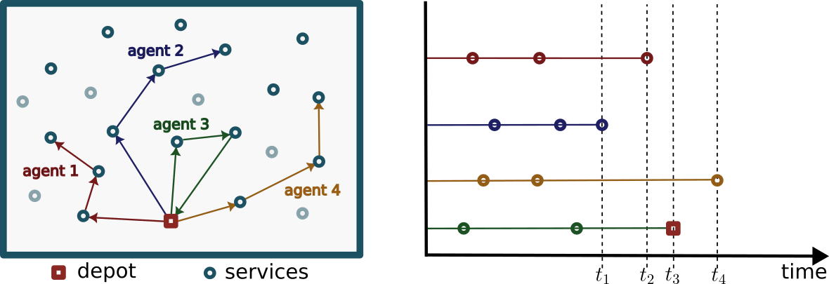
Figure 2.1: Illustration of a multi-agent VRP instance with four vehicles (left) and the corresponding timeline (right). All vehicles have completed a series of three actions steps. Since agents act asynchronously, the next agent to interact with the environment might have only partial information available.

These characteristics of the AEC game model are particularly crucial in VRP, and similar ideas were explored in Bono et al., (2020), where the authors presented a sequential multi-agent Markov decision process, to address multi-agent dynamic vehicle routing problems. In fact, for time-dependent VRPs, each agent (vehicle) action is extended in time, and, as a consequence, agents have to make decisions asynchronously. As a consequence, if the agents acted simultaneously, the relative timing of the events is lost, and learning policies in these environments might not apply effectively to real-world scenarios (Menda et al., (2018)). Furthermore, the various constraints in routing problems impose the creation of conflict resolution rules.

As an example, consider the problem illustrated in Figure 2.1. There are four agents who have already completed three steps in an environment where each service can only be performed by a single vehicle. If we consider the environment steps with agents acting simultaneously, internally, it must handle conflicting actions and apply some tiebreaker rule to determine each agent’s actions. This approach has two main drawbacks. First, once an agent’s action is selected, the environment’s state changes, leaving other agents to make decisions based on outdated observations (Terry et al., (2021)). Moreover, assuming simultaneous action by all agents does not translate directly into practical applications, where agents have to decide their actions at different times (Menda et al., (2018)). These issues are absent when agents operate sequentially, as decisions are made using the latest environmental observations and can take into account the other agents’ timelines. This led us to adopt the AEC model in the foundations of our library.

3 Multi-agent Environments for Vehicle Routing Problems (MAEnvs4VRP)

In this section, we outline the architecture of our library and the design of its API. In order to enhance design freedom and maintenance, we have opted to implement each environment independently while maintaining a consistent transversal structure.

3.1 MAEnvs4VRP modules

Every environment is constructed using four key functional modules: Instance Generator, Observations Generator, Agent Selector, and Rewards classes (Fig. 3.1). Each block operates independently of the others, managing a key element of the environment’s dynamics.

Figure 3.1: Schematic representation of the library architecture.

Instance Generator Class. This module is responsible for the definition of the problem’s sample space and the generation of instances. It allows for fast exploration of new instance distributions and straightforward adoption of standard benchmark instance data commonly used to evaluate VRP solvers. This aims at narrowing the gap between test beds for algorithm benchmarking used in RL and OR communities, Accorsi et al., (2022), allowing a more objective performance comparison on a common ground.

For each environment, we provide three implementations:

• ToyInstanceGenerator - generates a small toy instance for environment testing and debugging;

• InstanceGenerator - random instance generator, following, whenever possible, the sample space definition of a seminal paper for the particular VRP problem. Using this generator, we provide test and validation instance sets;

• BenchmarkInstanceGenerator - reads and parses standard OR community test benchmark instances into our environment instance data format;

Alongside methods handling the described functionalities, these classes include the augment_generate_instance method, which simplifies the addition of instance augmentations, allowing for the exploration of symmetries within the generated environments. Augmentation techniques have been successfully applied during training and inference to enhance policy and solutions quality (e.g. Kwon et al., (2020); Kim et al., (2022); Li et al., (2024)).

Observations class. One important aspect for the successful training of the agents is their ability to retrieve useful information from the environment in order to act on it. Maintaining an independent and customizable observation class empowers feature engineering and observation space exploration, opening the possibility of creating more aware and capable agents. It also enables the creation of versatile environments that can be easily adjusted to reflect both fully and partially observable scenarios (Albrecht et al., (2024)), depending on the specific practical application at hand. This class is responsible for computing the observations available to the active agent while interacting with the environment. There are five types of possible observations:

• nodes_static - nodes (depots and services) intrinsic observations (e.g. location, time window width, demands, profits, etc);

• nodes_dynamic - nodes (depots and services) step-dependent observations. Usually, these observations are computed in relation to the active agent (e.g. time used by the agent after node visit, time left for location opening, time left for location closing);

• agent - active agent-related observations (e.g. number of visited nodes, number of feasible nodes, current load, time available);

• other_agents - observations regarding all agents still active in the environment (e.g. location, time available, used capacity, distance to the active agent, time distance to the active agent);

• global - global state observations of the environment (e.g. number of completed services, number of used agents, total demand satisfied, total profit collected);

By default, for each environment, a wide set of generic and problem-specific observations are readily available.

Agent Selector class. Equivalent to PettingZoo’s, the Agent Selector class controls the selection of the next agent that will interact with the environment, through the _next_agent method. This is an important aspect in multi-agent problems, particularly in time-dependent ones, as it enables the exploration of different strategies for choosing agents. For a broader class of VRP problems, where time constraints or some form of randomness is present, more suitable agent selection functions, dependent on the state of the environment, can be designed or even learned.

Currently, Agent Selector classes available are AgentSelector, SmallestTimeAgentSelector and RandomSelector. In AgentSelector the generator steps through the active agents in a circular fashion until no more active agents are available. It always selects the same agent until that agent returns to the depot. Afterwards, it selects the next active agent and repeats the process until all agents are done, thus mimicking a single-agent environment. SmallestTimeAgentSelector selects the agent with the smallest acumulated time since departure from the depot (Bono et al., (2020)). This allowsto simulate an environment in which agents must act in real-time. Lastly, RandomSelector selects randomly between active agents.

Reward class.

Generally, the objective function to be optimized may differ significantly across various VRP types, contingent upon the specific application. Additionally, even for the same VRP, the literature might present diverse objective functions. For instance, in the Capacitated Vehicle Routing Problem with Time Windows (A.1), conventional objectives might include minimizing the total route distance, reducing the total number of vehicles, or optimizing a linear combination of these factors. To easily account for this variability in the objective function’s setup, the Reward class allows for a straightforward reward design through the get_reward method, enabling also a broader exploration of reward engineering.

In fact, to account for constraints violation (e.g. maximum allowed tour duration, time window violation, unvisited customers, etc.), the method returns for every environment step a reward and a penalty, Zhang et al., 2023a . The ability to define a penalty, alongside and separately from the reward, is especially beneficial for scenarios that aim at minimizing overall travel time or distance. This approach enables, on the implementation side, agents to have the freedom to decide whether to perform services or stay at the depot, without needing to force a minimum number of services.

Currently, each environment provides access to both dense rewards (available at every step of the environment) and sparse rewards (retrieved at the episode’s conclusion). The flexibility to choose the reward type expands the possibilities of downstream algorithm design.

3.2 Environments and API

In order to provide representative examples of various variants, we implemented environments contemplating hard and soft time windows constraints and single/multi-depot settings. Currently, the library offers seven off-the-shelf environments to simulate the following VRP: Capacitated Vehicle Routing Problem with soft and hard time windows, Team Orienteering Problem, Pickup and Delivery Problem, Split Delivery Vehicle Routing Problem, Prize-Collecting Vehicle Routing Problem and Multi-depot Vehicle Routing Problem. In line with Accorsi et al., (2022), precise definitions of each environment, along with their observations and rewards, are provided in Appendix A.

Our library manages all data through TensorDicts, a dictionary-like structure introduced in TorchRL (Bou et al., (2023)). This allows for efficient tensor operations, streamlines data management, and supports the development of batched (vectorized) environments. As illustrated in Code snippet 3.2, a typical episode run follows the logic found in most standard RL APIs.

⬇

\parfrom maenvs4vrp.environments.cvrptw.env import Environment

from maenvs4vrp.environments.cvrptw.env_agent_selector import AgentSelector

from maenvs4vrp.environments.cvrptw.observations import Observations

from maenvs4vrp.environments.cvrptw.instances_generator import InstanceGenerator

from maenvs4vrp.environments.cvrptw.env_agent_reward import DenseReward

\pargen = InstanceGenerator()

obs = Observations()

sel = AgentSelector()

rew = DenseReward()

\parenv = Environment(instance_generator=gen,

obs_builder=obs,

agent_selector=sel,

reward_evaluator=rew,

seed=0)

\parenv_state : TensorDict = env.reset()

while not env_state["done"].all():

env_state = env.sample_action(env_state)

env_state = env.step(env_state)

Figure 3.2: Basic API usage example. Here, env_state is a data container TensorDict.

The environment is set up using the reset method. This method internally generates a td_state state dictionary which contains all the details about nodes and agents. It also selects the first agent to act and determines its observations through the method observe. This method provides the environment state with observations, along with the action and agents’ masks. A TensorDict is returned which contains keys such as agent index, observations, reward, penalty, and done.

Following initialization, the loop of agent selection, observation gathering, action determination, and environment updating continues until all vectorized environments are complete. This method naturally and clearly depicts the step-by-step process the agents use in their interaction with the environment. Specifically, after an agent is selected, it observes the current state of the environment; based on these observations, an action is determined and executed (step), updating the environment’s state (and any other agents within it).

An additional feature in our environments is the stats_report method. It is used when all agents are done, and returns a dictionary with episodic relevant information, e.g. final episodic reward and penalties, solution statistics, etc. This information is integrated, along with complementary agent information, in the last returned info dictionary.

4 Experiments and benchmark results

We obtained baseline performance values for a subset of available environments by training the MARDAM multi-agent network model (Bono et al., (2020)). This model, whose implementation was made publicly available by the authors, is a variation of the Attention model (Kool et al., (2019)), and was designed so that it could handle dynamic multi-agent routing problems, where decisions have to be made online. It combines the standard attention node encoding block with a multi-head attention layer to encode the vehicle fleet.

To fully leverage the information available on each agent’s observations before selecting the next action, we developed an extension of the previous model, termed the Multi-Agent Dynamic Attention Model (MADyAM). At each environment step, the model relies on the current agent state and two dynamic encoding blocks, one for nodes and one for the vehicle fleet, allowing for integrating updated features at every stage of the solution construction process (see Appendix B for a detailed description of the neural network model architecture).

We release all baseline models with training code and pre-trained checkpoints. In addition, for each environment, we provide a validation set comprised $2048$ instances with $50$ and $100$ services to enable an objective comparison between current and future approaches.

4.1 Experimental setup

In our experiments, we focus on CVRTPTW, TOPTW, PCVRPTW and MDVRPTW problems. For each of these VRPs, we train models in environments using two different agent selection strategies: sequential agent selection, thus simulating a single agent with multiple trips to the depot, and smallest time agent selection, similar to Bono et al., (2020), simulating an online setting.

For the baseline performance study, we use environments comprising $50$ and $100$ services. We use a fleet of $5$ vehicles for both the TOPTW and the PCVRPTW problems. In the case of CVRTPTW, $25$ vehicles were used, while for MDVRPTW, the configuration included $5$ depots, each equipped with $5$ vehicles. For a detailed description of the rewards and observations used by the agents, see Appendix A.

Training. For training the neural solvers, we follow most setups in (Bono et al., (2020)). We train all models with REINFORCE algorithm (Williams, (1992)) with critic baseline. We use Adam optimizer (Kingma and Ba, (2015)), with learning rate of $1e-4$ for the policy network and $1e-3$ for the critic. The models were trained for 100 epochs, each containing 2500 batches of size 512 training instances (i.e., 128M training instances in total).

We also compute baseline values with the state-of-the-art VRP solver Pyvrp, Wouda et al., (2024). This is a freely available high-performance VRP solver that achieves state-of-the-art results that support these problems off-the-shelf. For PyVRP, we multiply all float inputs by $10^{7}$ before rounding to integers and running the solver for 60 seconds.

All experiments were performed on a 2 $\times$ Nvidia GeForce RTX 4090 (GPU) and a 13^th Gen. Intel Core i9-13900 $\times$ 32 (CPU).

4.2 Experimental results

For every environment, we report the score gap to the PyVRP solver result in the benchmark instances. We define the score gap to the PyVRP solver as

$$gap=\frac{score_{model}-score_{PyVRP}}{score_{PyVRP}}\times 100.$$

Notice that for CVRPTW and MDVRPTW the gap will be negative if the model outperforms PyVRP solver. On the other hand, for TOPTW and PCVRPTW gap will be positive if the model outperforms PyVRP solver.

The baseline results obtained, as shown in Table 4.1, indicate that the poorest performance consistently occurs when models are trained under an online framework with smallest time agent selection. This setup requires that agents master asynchronous collaboration, considerably complicating the task. This underscores the critical need for authentic multi-agent simulators that aid in investigating and devising methods tailored to the unique challenges of multi-agent scenarios.

problem method agent selection 50 services 100 services av. obj. av. $\#$ agents gap ($\%$) av. obj. av. $\#$ agents gap ($\%$) CVRPTW $\downarrow$ PyVRP - 14.478 9.6 $-$ 24.493 16.9 $-$ MARDAM single agent 16.499 11.0 14.0 29.828 19.5 21.8 MADyAM 16.020 10.8 10.7 27.413 18.9 11.9 MARDAM smallest time 18.787 12.1 29.8 36.993 25.0 51.0 MADyAM 18.450 11.9 27.4 31.827 20.7 29.9 TOPTW $\uparrow$ PyVRP - 33.245 5.0 $-$ 39.984 5.0 $-$ MARDAM single agent 31.870 5.0 -4.1 39.251 5.0 -1.8 MADyAM 32.159 5.0 -3.3 39.710 5.0 -0.7 MARDAM smallest time 31.833 5.0 -4.2 39.026 5.0 -2.4 MADyAM 31.927 5.0 -4.0 39.407 5.0 -1.4 PCVRPTW $\uparrow$ PyVRP - 26.653 5.0 $-$ 35.534 5.0 $-$ MARDAM single agent 24.226 5.0 -9.1 32.325 5.0 -9.0 MADyAM 24.618 5.0 -7.6 32.907 5.0 -7.4 MARDAM smallest time 23.593 5.0 -11.5 31.309 5.0 -11.9 MADyAM 24.388 5.0 -8.5 32.706 5.0 -8.0 MDVRPTW $\downarrow$ PyVRP - 8.928 10.5 $-$ 15.224 17.9 $-$ MARDAM single agent 14.534 11.8 62.8 34.869 19.6 129.0 MADyAM 10.312 12.7 15.5 17.530 19.1 15.1 MARDAM smallest time 16.196 13.7 81.4 26.824 17.7 76.2 MADyAM 11.538 13.5 29.2 19.720 20.8 29.5

Table 4.1: Baseline values obtained, using greedy inference, for each problem validation set, training MARDAM and MADyAM models with single and smallest time agent selection strategies. For problems with $\uparrow$, higher objective values are better, and for $\downarrow$, lower objective values are better.

Analyzing the results across the various problems, we see that for TOPTW and PCVRPTW the average absolute gap is considerably smaller than for the other two problems, $5.9\%$ versus $39.7\%$ for CPRPTW and MDVRPTW. This difference is mainly due to two factors. In fact, for these problems, the number of agents used is smaller ($5$ versus $25$), and there are no penalties for not attending services, which facilitates learning.

In the CPRPTW and MDVRPTW problems, the evaluated baseline models exhibited inferior performance. This is in part because these environments involve a larger number of agents, making it more challenging for them to learn effective collaboration. Specifically, in such settings, agents are required to learn how to minimize the total distance traveled, while simultaneously ensuring the fulfillment of all services and preventing any penalties by the episode’s end. Consequently, some agents may inevitably decide to remain at the depot. For example, Figure 4.1 shows that in the CVRPTW scenario, the MARDAM model agents were unable to learn the strategy of staying in the depot, which resulted in suboptimal final solutions. Conversely, in the MDVRPTW scenario, this skill was acquired around epoch $35$, resulting in a significant increase in return. This observation, also noted in Bono et al., (2020), indicates that exploring approaches to improve inter-agent communication could potentially enhance collaboration and solution quality.

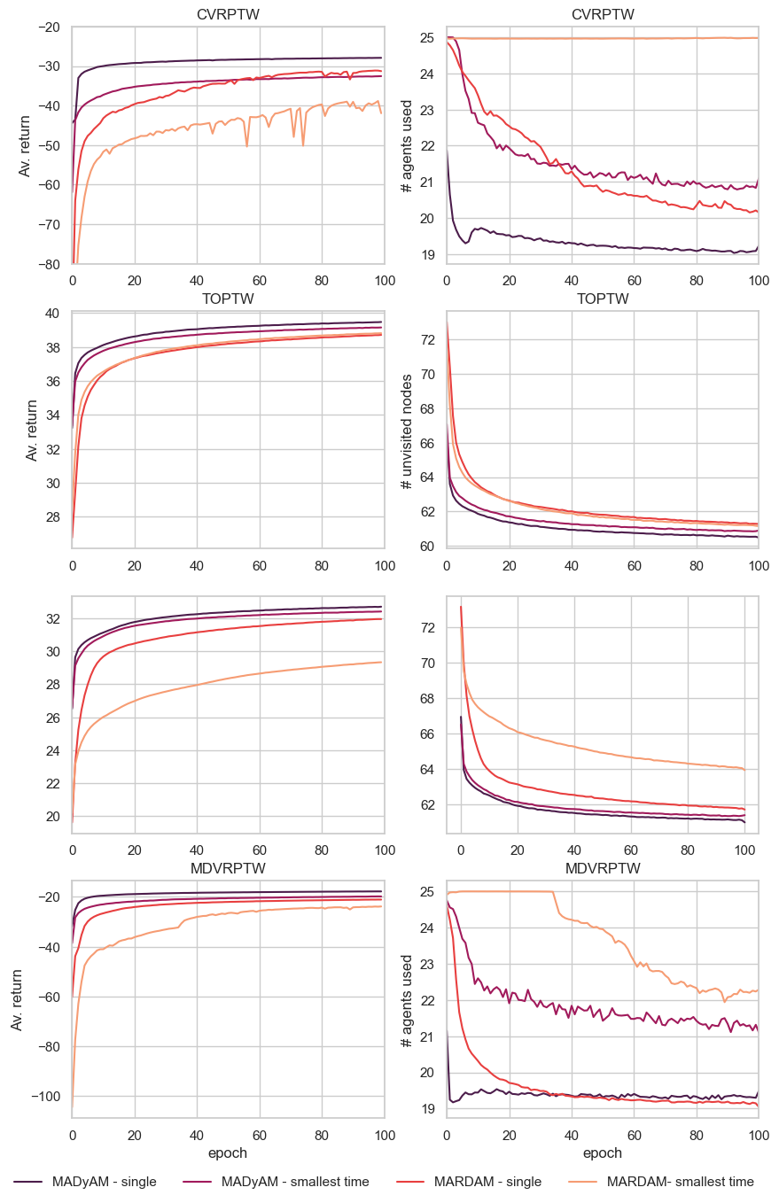
Figure 4.1: Evolution of models performance during training, using single and smallest time agent selection strategies, averaged by epoch. Each problem as 100 services. For the CVRPTW the fleet has 25 vehicles, and for both TOPTW and PCVRPTW 5 vehicles.

5 Discussion and future developments

Here we introduce MAEnvs4VRP, an open-source library featuring a multi-agent environment designed to simulate vehicle routing problems. Not only does it provide a set of ready-to-use environments for classical VRP, but it also offers a flexible framework that facilitates easy customization and the implementation of new VRP environments in both online and offline setups. With a modular architecture, a simple API and detailed accompanying documentation, it enhances its adoption by researchers. Along with detailing the library, we present baseline experimental results, that we hope will motivate the exploration of new approaches and multi-agent algorithms aimed at tackling routing problems through reinforcement learning. In the near future, we intend to implement environments for dynamic and stochastic problems, thus expanding the class of problems covered.

The project source code can be found in GitHub .

Appendix A Vehicle Routing Problems Environments

In this section, following the guidelines of Accorsi et al. (Accorsi et al., (2022)), we present a formal problem definition and objective description of the implemented environments.

A.1 Capacitated Vehicle Routing Problem with Time Windows (CVRPTW)

Problem definition. On the CRPTW we have a fleet of vehicles to serve a set of customers with known demands. Each customer can only be served once by a single vehicle. The service must be carried out within a defined time window and respecting the vehicle’s capacities (see Solomon, (1987)). Concretely, an instance consists of a fleet of $V$ homogeneous vehicles, a set of $n$ nodes $\{\mathrm{n}_{i}\}_{i=1}^{n}$, a depot and a set of $n-1$ services, with their corresponding coordinates $x_{i}\in\mathbb{R}^{2}$, a $n\times n$ symmetric matrix $T$ with travel time between each pair of locations, a quantity $d_{i}$ that specifies the demand for some resource by each customer $\mathrm{n}_{i}$, and the maximum quantity, $Q$, of the resource that a vehicle can carry. In addition, each node $\mathrm{n}_{i}$ is specified with a visiting time window $[o_{i},c_{i}]$ with opening time and closing time, and service time $s_{i}$. Unless otherwise stated, time window constraints are considered hard constraints, i.e. a vehicle is allowed to arrive at a customer location before its opening time, but it must wait to make the delivery. If it arrives after its closing time, it’s not allowed to serve the respective customer.

Observations.

• Nodes static features: node coordinates, time window, demand, service time, bool is depot;

• Nodes dynamic features: time to open, time to close, arriving time at note, time to open after step, time to close after step, time to end tour after step, fraction of time elapsed after step;

• Agent features: present location coordinates, fraction of time elapsed, fraction of current load, time to depot, fraction of feasible nodes, fraction of visited nodes

• Other agents features: present location coordinates, fraction of time elapsed, fraction of current load, time to depot, fraction of feasible nodes, fraction of visited nodes, distance to active agent, time difference to active agent, bool was last active agent;

• Global features: fraction of served demands, current fraction of fleet capacity, fraction of done agents;

Reward.

• Dense: At every step, the reward is the negative distance traveled by the agent. At the end of the episode, a penalty is given equaling $10$ times the negative distance from the depot to the not attended services.

• Sparse: The reward is 0 in all steps except the last. At the end of the episode, the reward is the negative of the sum of the distances of the routes traveled by all agents minus the sum of the penalties for each service not performed. The penalty for a not-performed service is $10$ times the distance from the depot to that service.

A.2 Capacitated Vehicle Routing Problem with Soft Time Windows (CVRPSTW)

Problem definition. In this variation of the CVRPTW, time window constraints are relaxed and can be violated at a penalty cost (usually linear, proportional to the interval between opening/closing times and vehicle arrival. Although the penalty function can be defined in several ways, we consider the formulation studied in Figliozzi, (2010)). Concretely, the time window violation cannot exceed $P_{max}$, and consequently, for each customer, we can enlarge its time window to $[o_{i}-P_{max},c_{i}+P_{max}]=[o^{s}_{i},c^{s}_{i}]$ outside which the service cannot be performed. When a vehicle arrives at a customer at time $t_{i}\in[o^{s}_{i},c^{s}_{i}]$, it can have an early arrival penalty cost of $p_{e}\max(o_{i}-t_{i},0)$ and a late arrival penalty cost of $p_{l}\max(t_{i}-c_{i},0)$.

Furthermore, the vehicle’s maximum waiting time at any customer, $W_{max}$, is imposed. That is, the vehicles can only arrive at each customer after $o_{i}-P_{max}-W_{max}$, so that its waiting time doesn’t exceed $W_{max}$.

Observations.

• Nodes static features: node coordinates, time window, demand, service time, bool is depot;

• Nodes dynamic features: time to open, time to close, arriving time at note, time to open after step, time to close after step, time to end tour after step, fraction of time elapsed after step;

• Agent features: present location coordinates, fraction of time elapsed, fraction of current load, time to depot, fraction of feasible nodes, fraction of visited nodes

• Other agents features: present location coordinates, fraction of time elapsed, fraction of current load, time to depot, fraction of feasible nodes, fraction of visited nodes, distance to active agent, time difference to active agent, bool was last active agent;

• Global features: fraction of served demands, current fraction of fleet capacity, fraction of done agents;

Reward.

• Dense: At every step, the reward is the negative distance traveled by the agent plus the penalty for early and late time window arrival. At the end of the episode, a penalty is given equaling $10$ times the negative distance from the depot to the not attended services.

• Sparse: The reward is 0 in all steps except the last. At the end of the episode, the reward is the negative of the sum of the distances of the routes traveled by all agents minus the sum of the penalties for each service not performed and time window violation. The penalty for a not-performed service is $10$ times the distance from the depot to that service.

A.3 Team Orienteering Problem with Time Windows (TOPTW)

Problem definition. In a TOPTW instance, a set of $n$ nodes, $\{\mathrm{n}_{i}\}_{i=1}^{n}$ with their corresponding coordinates $x_{i}\in\mathbb{R}^{2}$ and a $n\times n$ symmetric matrix $T$ with travel time between each pair of locations, are given. Every node $\mathrm{n}_{i}$ has a positive score or profit, $p_{i}$, a visiting time window $[o_{i},c_{i}]$ with opening time (the earliest a visit can start) and closing time (the latest time for which a visit can start), and duration of visit $d_{i}$. Without loss of generality, we can assume that $\mathrm{n}_{1}$ is the starting and ending location for every route. The objective is to find $m$ routes with the maximum possible sum of scores, without repeating visits, starting each route on or after a given time $t_{start}$ and ending before time $t_{end}$ (see Vansteenwegen and Gunawan, (2019)).

Observations.

• Nodes static features: node coordinates, time window, profit, service time, bool is depot;

• Nodes dynamic features: time to open, time to close, arriving time at note, time to open after step, time to close after step, time to end tour after step, fraction of time elapsed after step;

• Agent features: present location coordinates, fraction of time elapsed, time to depot;

• Other agents features: present location coordinates, fraction of time elapsed, time to depot, fraction of feasible nodes, fraction of visited nodes, distance to active agent, time difference to active agent, bool was last active agent;

• Global features: fraction of profits collected, fraction of done agents;

Reward.

• Dense: At every step, the reward is the profit collected by the agent.

• Sparse: The reward is 0 in all steps except the last. At the end of the episode, the reward is the sum of all agent’s collected profits.

A.4 Pickup and Delivery Problem with Time Windows (PDPTW)

Problem definition. In the pickup and delivery problem with time windows (see Dumas et al., (1991)), a fleet of vehicles with uniform capacity has to collect and deliver items to satisfy pairs of customers, respecting their visiting time window. Concretely, an instance consists of a fleet of $V$ homogeneous vehicles with maximum capacity $Q$. A set of $2n+1$ nodes $\{\mathrm{n}_{i}\}_{i=1}^{2n+1}$, a depot and a set $\{1,\ldots,n\}$ of pickup services and their corresponding $\{n+1,\ldots,2n\}$ delivery services, with coordinates $x_{i}\in\mathbb{R}^{2}$, a $2n+1\times 2n+1$ symmetric matrix $T$ with travel time between each pair of locations. Each customer with a pick-up service has a quantity $d_{i}$ to be delivered to a particular customer $\mathrm{n}_{n+i}$. In addition, each node $\mathrm{n}_{i}$ is specified with a visiting time window $[o_{i},c_{i}]$ with opening time and closing time, and service time $s_{i}$.

Observations.

• Nodes static features: node coordinates, time window, demand, service time, bool is depot, bool is pickup, bool is delivery;

• Nodes dynamic features: time to open, time to close, arriving time at note, time to open after step, time to close after step, time to end tour after step, fraction of time elapsed after step;

• Agent features: present location coordinates, fraction of time elapsed, fraction of current load, time to depot, fraction of feasible nodes, fraction of visited nodes

• Other agents features: present location coordinates, fraction of time elapsed, fraction of current load, time to depot, fraction of feasible nodes, fraction of visited nodes, distance to active agent, time difference to active agent, bool was last active agent;

• Global features: fraction of served demands, current fraction of fleet capacity, fraction of done agents;

Reward.

• Dense: At every step, the reward is the negative distance traveled by the agent. At the end of the episode, a penalty is given equaling $10$ times the negative distance from the depot to the not attended services.

• Sparse: The reward is 0 in all steps except the last. At the end of the episode, the reward is the negative of the sum of the distances of the routes traveled by all agents minus the sum of the penalties for each service not performed. The penalty for a not-performed service is $10$ times the distance from the depot to that service.

A.5 Split Delivery Vehicle Routing Problem with Time Windows (SDVRPTW)

Problem definition. The Split Delivery Vehicle Routing Problem with Time Windows (SDVRPTW) is a generalization of the CVRPTW where each customer can be visited more than once by several vehicles and a fraction of the demand can be met (see Bianchessi et al., (2019)).

Observations.

• Nodes static features: node coordinates, time window, demand, service time, bool is depot;

• Nodes dynamic features: time to open, time to close, arriving time at note, time to open after step, time to close after step, time to end tour after step, fraction of time elapsed after step;

• Agent features: present location coordinates, fraction of time elapsed, fraction of current load, time to depot, fraction of feasible nodes, fraction of visited nodes

• Other agents features: present location coordinates, fraction of time elapsed, fraction of current load, time to depot, fraction of feasible nodes, fraction of visited nodes, distance to active agent, time difference to active agent, bool was last active agent;

• Global features: fraction of served demands, current fraction of fleet capacity, fraction of done agents;

Reward.

• Dense: At every step, the reward is the negative distance traveled by the agent. At the end of the episode, a penalty is given equaling $10$ times the negative distance from the depot to the not attended services.

• Sparse: The reward is 0 in all steps except the last. At the end of the episode, the reward is the negative of the sum of the distances of the routes traveled by all agents minus the sum of the penalties for each service not performed. The penalty for a not-performed service is $10$ times the distance from the depot to that service.

A.6 Prize-Collecting Vehicle Routing Problem with Time Windows (PCVRPTW)

Problem definition. This version of the CVRPTW does not require visiting all clients. Instead, each client has a prize (profit) that is collected upon visitation. The objective is to minimize the total combined traveled time of all vehicle routes while maximizing the collected prizes.

Observations.

• Nodes static features: node coordinates, time window, demand, prizes, service time, bool is depot;

• Nodes dynamic features: time to open, time to close, arriving time at note, time to open after step, time to close after step, time to end tour after step, fraction of time elapsed after step;

• Agent features: present location coordinates, fraction of time elapsed, fraction of current load, time to depot, fraction of feasible nodes, fraction of visited nodes

• Other agents features: present location coordinates, fraction of time elapsed, fraction of current load, time to depot, fraction of feasible nodes, fraction of visited nodes, distance to active agent, time difference to active agent, bool was last active agent;

• Global features: fraction of served demands, fraction of collected prizes, current fraction of fleet capacity, fraction of done agents;

Reward.

• Dense: At every step, the reward is the negative distance traveled plus the client prize collected by the agent.

• Sparse: The reward is 0 in all steps except the last. At the end of the episode, the reward is the negative of the sum of the distances of the routes traveled plus the sum of all agents collected prizes.

A.7 Multi-depot Vehicle Routing Problem with Time Windows (MDVRPTW)

The Multi-depot Vehicle Routing Problem with Time Windows (MDVRPTW) is a generalization of the CVRPTW with multiple depots. Each depot has its own set of vehicles that depart and must return to it.

Observations.

• Nodes static features: node coordinates, time window, demand, service time, bool is depot;

• Nodes dynamic features: time to open, time to close, arriving time at note, time to open after step, time to close after step, time to end tour after step, fraction of time elapsed after step;

• Agent features: present location coordinates, fraction of time elapsed, fraction of current load, time to depot, fraction of feasible nodes, fraction of visited nodes

• Other agents features: present location coordinates, fraction of time elapsed, fraction of current load, time to depot, fraction of feasible nodes, fraction of visited nodes, distance to active agent, time difference to active agent, bool was last active agent;

• Global features: fraction of served demands, current fraction of fleet capacity, fraction of done agents;

Reward.

• Dense: At every step, the reward is the negative distance traveled by the agent. At the end of the episode, a penalty is given equaling $10$ times the negative distance from the depot to the not attended services.

• Sparse: The reward is 0 in all steps except the last. At the end of the episode, the reward is the negative of the sum of the distances of the routes traveled by all agents minus the sum of the penalties for each service not performed. The penalty for a not-performed service is $10$ times the distance from the depot to that service.

Appendix B Multi-Agent Multi-Dynamic Attention Model (MADyAM)

Designed to be applied to multi-agent problems, the MARDAM model,(Bono et al., (2020)), is an adaptation of the Attention model of Kool et al., (2019). In order to leverage the MARDAM model to better address problems with dynamic time-dependent constraints, we redesign it to include the changes on the multi-head self-attention glimpse layer proposed in Kool et al., (2019); Berto et al., (2023), see figure B.1.

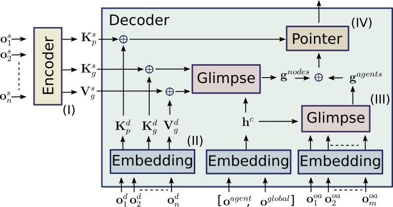
Figure B.1: Illustration of MADyAM architecture. (I) Encoding block consisting of $n$ transformer encoder layers; (II) Embedding layers responsible for the projection of the observation into the embedding space; (III) Attention glimpse layer; (IV) Pointer layer outputting actions probabilities.

As illustrated in figure B.1, MADyAM architecture is able to process the five types of possible agent environment observations, i.e. nodes_static ($\mathbf{o}^{s}$), nodes_dynamic ($\mathbf{o}^{d}$), agent ($\mathbf{o}^{agent}$), other_agents ($\mathbf{o}^{oa}$) and global ($\mathbf{o}^{global}$).

Equivalently to Kool et al., (2019); Bono et al., (2020), it has an encoding block (I), made up of $N$ layers of a transformer encoder (Vaswani, (2017)) (in our case $N=3$). This encoding maps the static nodes observations $\mathbf{o}_{i}^{s}$ into cached keys and values vectors. Subsequently, during the decoding step, these cached keys and value vectors will be updated, (II), with the projections into the embedding space of dynamic node observations $\mathbf{o}_{i}^{d}$:

$$\mathbf{V}_{g}=\mathbf{V}_{g}^{s}+\mathbf{V}_{g}^{d},\quad\mathbf{K}_{g}=\mathbf{K}_{g}^{s}+\mathbf{K}_{g}^{d},\quad\mathbf{K}_{p}=\mathbf{K}_{p}^{s}+\mathbf{K}_{p}^{d},$$

The context vector, $\mathbf{h}^{c}$, is the embedding of global and acting agent observations. This vector is used to compute a glimpse (III) into nodes ($\mathbf{g}^{nodes}$) and other agents ($\mathbf{g}^{agents}$) features. The sum of these vectors, ($\mathbf{g}^{nodes}+\mathbf{g}^{agents}$) is then fed into the attention pointer head (IV) to obtain the next action probabilities. For more details about layers definitions and the Attention and MARDAM models, see Kool et al., (2019); Bono et al., (2020).

References

- Accorsi et al., (2022) Accorsi, L., Lodi, A., and Vigo, D. (2022). Guidelines for the computational testing of machine learning approaches to vehicle routing problems. Operations Research Letters, 50(2):229–234.
- Albrecht et al., (2024) Albrecht, S. V., Christianos, F., and Schäfer, L. (2024). Multi-Agent Reinforcement Learning: Foundations and Modern Approaches. MIT Press.
- Arishi and Krishnan, (2023) Arishi, A. and Krishnan, K. (2023). A multi-agent deep reinforcement learning approach for solving the multi-depot vehicle routing problem. Journal of Management Analytics, 10(3):493–515.
- Balaji et al., (2019) Balaji, B., Bell-Masterson, J., Bilgin, E., Damianou, A., Garcia, P. M., Jain, A., Luo, R., Maggiar, A., Narayanaswamy, B., and Ye, C. (2019). Orl: Reinforcement learning benchmarks for online stochastic optimization problems. arXiv preprint arXiv:1911.10641.
- Bello et al., (2017) Bello, I., Pham, H., Le, Q. V., Norouzi, M., and Bengio, S. (2017). Neural Combinatorial Optimization with Reinforcement Learning. Proceedings of the 5th International Conference on Learning Representations (ICLR).
- (6) Berto, F., Hua, C., Luttmann, L., Son, J., Park, J., Ahn, K., Kwon, C., Xie, L., and Park, J. (2024a). Parco: Learning parallel autoregressive policies for efficient multi-agent combinatorial optimization. arXiv preprint arXiv:2409.03811.
- Berto et al., (2023) Berto, F., Hua, C., Park, J., Kim, M., Kim, H., Son, J., Kim, H., Kim, J., and Park, J. (2023). RL4CO: an extensive reinforcement learning for combinatorial optimization benchmark. arXiv preprint arXiv:2306.17100.
- (8) Berto, F., Hua, C., Zepeda, N. G., Hottung, A., Wouda, N., Lan, L., Tierney, K., and Park, J. (2024b). Routefinder: Towards foundation models for vehicle routing problems. arXiv preprint arXiv:2406.15007.
- Bettini et al., (2024) Bettini, M., Prorok, A., and Moens, V. (2024). Benchmarl: Benchmarking multi-agent reinforcement learning. Journal of Machine Learning Research, 25(217):1–10.
- Biagioni et al., (2022) Biagioni, D., Tripp, C. E., Clark, S., Duplyakin, D., Law, J., and John, P. C. S. (2022). graphenv: a python library for reinforcement learning on graph search spaces. Journal of Open Source Software, 7(77):4621.
- Bianchessi et al., (2019) Bianchessi, N., Drexl, M., and Irnich, S. (2019). The split delivery vehicle routing problem with time windows and customer inconvenience constraints. Transportation Science, 53(4):1067–1084.
- Bonnet et al., (2023) Bonnet, C., Luo, D., Byrne, D., Surana, S., Coyette, V., Duckworth, P., Midgley, L. I., Kalloniatis, T., Abramowitz, S., Waters, C. N., Smit, A. P., Grinsztajn, N., Sob, U. A. M., Mahjoub, O., Tegegn, E., Mimouni, M. A., Boige, R., de Kock, R., Furelos-Blanco, D., Le, V., Pretorius, A., and Laterre, A. (2023). Jumanji: a diverse suite of scalable reinforcement learning environments in jax.
- Bono et al., (2020) Bono, G., Dibangoye, J. S., Simonin, O., Matignon, L., and Pereyron, F. (2020). Solving multi-agent routing problems using deep attention mechanisms. IEEE Transactions on Intelligent Transportation Systems, 22(12):7804–7813.
- Bou et al., (2023) Bou, A., Bettini, M., Dittert, S., Kumar, V., Sodhani, S., Yang, X., Fabritiis, G. D., and Moens, V. (2023). Torchrl: A data-driven decision-making library for pytorch.
- Braekers et al., (2016) Braekers, K., Ramaekers, K., and Van Nieuwenhuyse, I. (2016). The vehicle routing problem: State of the art classification and review. Computers & industrial engineering, 99:300–313.
- Brockman et al., (2016) Brockman, G., Cheung, V., Pettersson, L., Schneider, J., Schulman, J., Tang, J., and Zaremba, W. (2016). Openai gym. arXiv preprint arXiv:1606.01540.
- Dumas et al., (1991) Dumas, Y., Desrosiers, J., and Soumis, F. (1991). The pickup and delivery problem with time windows. European Journal of Operational Research, 54(1):7–22.
- Figliozzi, (2010) Figliozzi, M. A. (2010). An iterative route construction and improvement algorithm for the vehicle routing problem with soft time windows. Transportation Research Part C: Emerging Technologies, 18(5):668–679. Applications of Advanced Technologies in Transportation: Selected papers from the 10th AATT Conference.
- Fuertes et al., (2023) Fuertes, D., del Blanco, C. R., Jaureguizar, F., and García, N. (2023). Solving the team orienteering problem with transformers. arXiv preprint arXiv:2311.18662.
- Guo et al., (2023) Guo, F., Wei, Q., Wang, M., Guo, Z., and Wallace, S. W. (2023). Deep attention models with dimension-reduction and gate mechanisms for solving practical time-dependent vehicle routing problems. Transportation Research Part E: Logistics and Transportation Review, 173:103095.
- Hu et al., (2023) Hu, S., Zhong, Y., Gao, M., Wang, W., Dong, H., Liang, X., Li, Z., Chang, X., and Yang, Y. (2023). Marllib: A scalable and efficient multi-agent reinforcement learning library. Journal of Machine Learning Research, 24(315):1–23.
- Hubbs et al., (2020) Hubbs, C. D., Perez, H. D., Sarwar, O., Sahinidis, N. V., Grossmann, I. E., and Wassick, J. M. (2020). Or-gym: A reinforcement learning library for operations research problems.
- Kim et al., (2022) Kim, M., Park, J., and Park, J. (2022). Sym-nco: Leveraging symmetricity for neural combinatorial optimization. Advances in Neural Information Processing Systems, 35:1936–1949.
- Kingma and Ba, (2015) Kingma, D. P. and Ba, J. (2015). Adam: A method for stochastic optimization. International Conference on Learning Representations (ICLR), abs/1412.6980.
- Kool et al., (2019) Kool, W., Van Hoof, H., and Welling, M. (2019). Attention, learn to solve routing problems! 7th International Conference on Learning Representations, ICLR 2019, pages 1–25.
- Kwon et al., (2020) Kwon, Y.-D., Choo, J., Kim, B., Yoon, I., Gwon, Y., and Min, S. (2020). Pomo: Policy optimization with multiple optima for reinforcement learning. Advances in Neural Information Processing Systems, 33:21188–21198.
- Li et al., (2022) Li, B., Wu, G., He, Y., Fan, M., and Pedrycz, W. (2022). An overview and experimental study of learning-based optimization algorithms for the vehicle routing problem. IEEE/CAA Journal of Automatica Sinica, 9(7):1115–1138.
- Li et al., (2024) Li, J., Niu, Y., Zhu, G., and Xiao, J. (2024). Solving pick-up and delivery problems via deep reinforcement learning based symmetric neural optimization. Expert Systems with Applications, 255:124514.
- (29) Liu, F., Lin, X., Zhang, Q., Tong, X., and Yuan, M. (2024a). Multi-task learning for routing problem with cross-problem zero-shot generalization. arXiv preprint arXiv:2402.16891.
- (30) Liu, Q., Liu, C., Niu, S., Long, C., Zhang, J., and Xu, M. (2024b). 2d-ptr: 2d array pointer network for solving the heterogeneous capacitated vehicle routing problem. In Proceedings of the 23rd International Conference on Autonomous Agents and Multiagent Systems, pages 1238–1246.
- Mazyavkina et al., (2021) Mazyavkina, N., Sviridov, S., Ivanov, S., and Burnaev, E. (2021). Reinforcement learning for combinatorial optimization: A survey. Computers & Operations Research, 134:105400.
- Menda et al., (2018) Menda, K., Chen, Y.-C., Grana, J., Bono, J. W., Tracey, B. D., Kochenderfer, M. J., and Wolpert, D. (2018). Deep reinforcement learning for event-driven multi-agent decision processes. IEEE Transactions on Intelligent Transportation Systems, 20(4):1259–1268.
- Mohanty et al., (2020) Mohanty, S. P., Nygren, E., Laurent, F., Schneider, M., Scheller, C. V., Bhattacharya, N., Watson, J. D., Egli, A., Eichenberger, C., Baumberger, C., Vienken, G., Sturm, I., Sartoretti, G., and Spigler, G. (2020). Flatland-rl : Multi-agent reinforcement learning on trains. ArXiv, abs/2012.05893.
- Nazari et al., (2018) Nazari, M., Oroojlooy, A., Snyder, L. V., and Takáč, M. (2018). Deep Reinforcement Learning for Solving the Vehicle Routing Problem. In Proceedings Neural Information Processing Systems (NIPS), pages 9839–9849.
- Pan and Liu, (2023) Pan, W. and Liu, S. Q. (2023). Deep reinforcement learning for the dynamic and uncertain vehicle routing problem. Applied Intelligence, 53(1):405–422.
- Paszke et al., (2019) Paszke, A., Gross, S., Massa, F., Lerer, A., Bradbury, J., Chanan, G., Killeen, T., Lin, Z., Gimelshein, N., Antiga, L., Desmaison, A., Köpf, A., Yang, E., DeVito, Z., Raison, M., Tejani, A., Chilamkurthy, S., Steiner, B., Fang, L., Bai, J., and Chintala, S. (2019). PyTorch: an imperative style, high-performance deep learning library. Curran Associates Inc., Red Hook, NY, USA.
- Raffin et al., (2021) Raffin, A., Hill, A., Gleave, A., Kanervisto, A., Ernestus, M., and Dormann, N. (2021). Stable-baselines3: Reliable reinforcement learning implementations. Journal of Machine Learning Research, 22(268):1–8.
- Shi and Niu, (2023) Shi, R. and Niu, L. (2023). A brief survey on learning based methods for vehicle routing problems. Procedia Computer Science, 221:773–780. Tenth International Conference on Information Technology and Quantitative Management (ITQM 2023).
- Shoham and Leyton-Brown, (2008) Shoham, Y. and Leyton-Brown, K. (2008). Multiagent systems: Algorithmic, game-theoretic, and logical foundations. Cambridge University Press.
- Solomon, (1987) Solomon, M. M. (1987). Algorithms for the vehicle routing and scheduling problems with time window constraints. Operations Research, 35(2):254–265.
- Terry et al., (2021) Terry, J., Black, B., Grammel, N., Jayakumar, M., Hari, A., Sullivan, R., Santos, L. S., Dieffendahl, C., Horsch, C., Perez-Vicente, R., Williams, N., Lokesh, Y., and Ravi, P. (2021). Pettingzoo: Gym for multi-agent reinforcement learning. In Ranzato, M., Beygelzimer, A., Dauphin, Y., Liang, P., and Vaughan, J. W., editors, Advances in Neural Information Processing Systems, volume 34, pages 15032–15043. Curran Associates, Inc.
- Thyssens et al., (2023) Thyssens, D., Dernedde, T., Falkner, J. K., and Schmidt-Thieme, L. (2023). Routing arena: A benchmark suite for neural routing solvers. arXiv preprint arXiv:2310.04140.
- Vansteenwegen and Gunawan, (2019) Vansteenwegen, P. and Gunawan, A. (2019). Orienteering Problems, Models and Algorithms for Vehicle Routing Problems with Profits. Springer, euro advan edition.
- Vaswani, (2017) Vaswani, A. (2017). Attention is all you need. Advances in Neural Information Processing Systems.
- Vinyals et al., (2015) Vinyals, O., Fortunato, M., and Jaitly, N. (2015). Pointer networks. In Cortes, C., Lawrence, N. D., Lee, D. D., Sugiyama, M., and Garnett, R., editors, Advances in Neural Information Processing Systems 28, pages 2692–2700. Curran Associates, Inc.
- Wan et al., (2023) Wan, C. P., Li, T., and Wang, J. M. (2023). Rlor: A flexible framework of deep reinforcement learning for operation research.
- Williams, (1992) Williams, R. J. (1992). Simple statistical gradient-following algorithms for connectionist reinforcement learning. Machine Learning, 8(3):229–256.
- Wouda et al., (2024) Wouda, N. A., Lan, L., and Kool, W. (2024). PyVRP: a high-performance VRP solver package. INFORMS Journal on Computing.
- Wu et al., (2024) Wu, X., Wang, D., Wen, L., Xiao, Y., Wu, C., Wu, Y., Yu, C., Maskell, D. L., and Zhou, Y. (2024). Neural combinatorial optimization algorithms for solving vehicle routing problems: A comprehensive survey with perspectives. arXiv preprint arXiv:2406.00415.
- Xiang et al., (2024) Xiang, C., Wu, Z., Tu, J., and Huang, J. (2024). Centralized deep reinforcement learning method for dynamic multi-vehicle pickup and delivery problem with crowdshippers. IEEE Transactions on Intelligent Transportation Systems, 25(8):9253–9267.
- Zhang et al., (2020) Zhang, K., He, F., Zhang, Z., Lin, X., and Li, M. (2020). Multi-vehicle routing problems with soft time windows: A multi-agent reinforcement learning approach. Transportation Research Part C: Emerging Technologies, 121:102861.
- (52) Zhang, Y., Bliek, L., da Costa, P., Afshar, R. R., Reijnen, R., Catshoek, T., Vos, D., Verwer, S., Schmitt-Ulms, F., Hottung, A., et al. (2023a). The first ai4tsp competition: Learning to solve stochastic routing problems. Artificial Intelligence, 319:103918.
- (53) Zhang, Z., Qi, G., and Guan, W. (2023b). Coordinated multi-agent hierarchical deep reinforcement learning to solve multi-trip vehicle routing problems with soft time windows. IET Intelligent Transport Systems, 17(10):2034–2051.
- (54) Zhou, G., Li, X., Li, D., and Bian, J. (2024a). Learning-based optimization algorithms for routing problems: Bibliometric analysis and literature review. IEEE Transactions on Intelligent Transportation Systems.
- (55) Zhou, J., Cao, Z., Wu, Y., Song, W., Ma, Y., Zhang, J., and Xu, C. (2024b). Mvmoe: Multi-task vehicle routing solver with mixture-of-experts. arXiv preprint arXiv:2405.01029.
- Zong et al., (2022) Zong, Z., Zheng, M., Li, Y., and Jin, D. (2022). Mapdp: Cooperative multi-agent reinforcement learning to solve pickup and delivery problems. In Proceedings of the AAAI Conference on Artificial Intelligence, volume 36, pages 9980–9988.