Topological Twisting of 4d $\mathcal{N}=2$ Supersymmetric Field Theories

Abstract

We discuss what topological data must be provided to define topologically twisted partition functions of four-dimensional $\mathcal{N}=2$ supersymmetric field theories. The original example of Donaldson-Witten theory depends only on the diffeomorphism type of the spacetime and ’t Hooft fluxes (characteristic classes of background gerbe connections, a.k.a. “one-form symmetry connections.”) The example of $\mathcal{N}=2^{*}$ theories shows that, in general, the twisted partition functions depend on further topological data. We describe topological twisting for general four-dimensional $\mathcal{N}=2$ theories and argue that the topological partition functions depend on (a): the diffeomorphism type of the spacetime, (b): the characteristic classes of background gerbe connections and (c): a “generalized spin-c structure,” a concept we introduce and define. The main ideas are illustrated with both Lagrangian theories and class $\mathcal{S}$ theories. In the case of class $\mathcal{S}$ theories of $A_{1}$ type, we note that the different $S$-duality orbits of a theory associated with a fixed UV curve $C_{g,n}$ can have different topological data.

November 21, 2024

1 Introduction

This paper discusses topological twisting of $d=4$ ${\cal N}=2$ field theories. The first example of such a theory was discovered by Witten Wit (88), an example which had momentous implications. The study of topologically twisted $d=4$ ${\cal N}=2$ field theories is interesting in physics because it provides examples of computable partition functions and correlation functions within nontrivial $d=4$ QFTs. These “topological correlators” have been interesting to mathematicians because they provide invariants of smooth four-manifolds. More precisely, they provide invariants of smooth four-manifolds equipped with extra topological data. One goal of this paper is to clarify exactly what that extra topological data is.

In Donaldson-Witten theory (based on $\mr{SU(2)}$ ${\cal N}=2$ supersymmetric Yang-Mills theory) the topological correlators only depend on the orientation and the diffeomorphism type of ${\mathbb{X}}$ and a choice of ’t Hooft flux for the gauge group. However, the example of ${\cal N}=2^{*}$ theories shows that in general, the correlators depend on further topological data. In this example, topological twisting requires the introduction of an “ultraviolet” spin${}^{\mr}{c}$ structure LMn (97); MM (21). (This UV spin${}^{\mr}{c}$ structure should not be confused with the IR spin${}^{\mr}{c}$ structures which are used to express the answer derived from an IR viewpoint as in MW (97)). This raises the question: How does one topologically twist an arbitrary $d=4$ ${\cal N}=2$ field theory, and what topological data do the correlators depend on? This paper answers that question for all $d=4$ ${\cal N}=2$ theories and illustrates the general construction for renormalizable Lagrangian theories and for some theories of class ${\cal S}$.

There are many viewpoints on what should be meant by the general notion of “topological twisting.” They all generalize the original example in Wit (88). It would be interesting to relate the twistings we describe to the general viewpoint advocated in ES (18); ESW (20); EGL (24).

We will view topological twisting as a specification of background fields such that a supersymmetry, denoted ${\cal Q}$, remains unbroken. Since we do not work in a Hamiltonian framework, we view the supersymmetry as an odd vectorfield on the supermanifold of field configurations. We assume ${\cal Q}$ is a scalar since general manifolds ${\mathbb{X}}$ do not possess covariantly constant vectors, spinors, etc. ${\cal Q}$ must square to zero on physical operators (and, in the Hamiltonian formulation, on states). For example, in a gauge theory, “physical operators” are the gauge invariant operators. In general, there can be different “inequivalent” topological twistings of a given theory. For example, there are, famously, several inequivalent twistings of ${\cal N}=4$ super Yang-Mills (SYM) VW (94) (which is a special case of an ${\cal N}=2$ SYM), as we recall in section 6.1. In our view, these are 3 inequivalent choices of background fields effecting a topological twisting.

The specification of background fields effecting a topological twisting will be given using the mathematical concept of transfer of structure group. Briefly, given a continuous homomorphism $\varphi:G_{1}\to G_{2}$ between topological groups one can define a functor $\varphi_{*}$ between categories (in fact, groupoids) of principal bundles with connection over ${\mathbb{X}}$ for the domain and codomain groups $G_{1}$ and $G_{2}$, respectively. Thus, if $(P_{1},\bm{\nabla}_{1})$ is a principal $G_{1}$-bundle over ${\mathbb{X}}$ with connection $\bm{\nabla}_{1}$ then $\varphi_{*}(P_{1},\bm{\nabla}_{1})$ will be a principal $G_{2}$-bundle over ${\mathbb{X}}$ with connection $\bm{\nabla}_{2}=\varphi_{*}\bm{\nabla}_{1}$. We explain this concept with various examples in Appendix B.

In section 2 we describe our general approach to topological twisting of a $d=4$ ${\cal N}=2$ field theory. We explain the implementation for any renormalizable Lagrangian theory in section 6 and for some class ${\cal S}$ theories in sections 8 and 9. We describe a twisting valid for generic masses (the background scalar vevs of flavor symmetry vectormultiplets). For special values of the background VM’s other topological twistings will exist.

In order to sharpen the main question above, we organize the correlators into a “function” (more precisely formal series) defined on the ${\cal Q}$-cohomology of the space of operators. This function will depend on continuous parameters and what we call the topological data. The topological data only depends on the (smooth) topology of ${\mathbb{X}}$.

In more technical terms, the ${\cal Q}$-cohomology of the space of (extended) observables will be denoted ${\cal O}$. Choosing a basis $O_{i}$ for the vector space ${\cal O}$ with dual basis $x^{i}$ for ${\cal O}^{\vee}$, we denote the generating function of the correlators as:

$$\mr{Z}^{\mr{tw}}(x)=\big{\langle}e^{\sum_{i}x^{i}O_{i}}\big{\rangle}~{}.$$ (1)

We view this as a “function” (actually, formal power series) of $x\in{\cal O}^{\vee}$. As we just mentioned, $\mr{Z}^{\mr{tw}}(x)$ will also depend on continuous parameters. Examples of such parameters include the superconformal couplings $\tau_{\mr{uv}}\in{\cal C}$, where ${\cal C}$ is the conformal manifold, and the mass parameters $m\in(\mathfrak{t}^{\mr{f}})^{\vee}$, where $\mathfrak{t}^{\mr{f}}$ is the Lie algebra of the group of global “flavor” symmetries. Such parameters should be viewed as background fields in the theory, and we will be interested in the ${\cal Q}$-invariant background parameters ${\cal F}^{{\cal Q}}$. The net result is that the generator of topological correlation functions is a function

$$\mr{Z}^{\mr{tw}}:{\cal O}^{\vee}\times{\cal F}^{{\cal Q}}\to\mathbb{C}~{}.$$ (2)

We will show that the function $\mr{Z}^{\mr{tw}}$ depends on the topological data:

1. The orientation and diffeomorphism type of ${\mathbb{X}}$.

2. ’t Hooft fluxes (i.e., background connections for “discrete 1-form symmetries”)

3. Generalized spin${}^{\mr}{c}$ structures.

and only depends on these data. No other choices of topological data are needed.

In Appendix C, we define the notion of a generalized spin${}^{\mr}{c}$ structure. (We focus on four dimensions. The generalization to other dimensions is obvious.) It is a (mild) generalization of the notion of a spin${}^{\mr}{c}$ structure. One replaces the $\mr{U(1)}$ “factor” in the definition of the spin${}^{\mr}{c}$ group by a general torus ${\mathbb{T}}$, and quotients by a finite Abelian subgroup of $\mr{Spin(4)}\times{\mathbb{T}}$ that projects to the ${\mathbb{Z}}_{2}$ subgroup of $\mr{Spin(4)}$ acting trivially on vectorial representations.

The general arguments of section 2 apply to all $d=4$ ${\cal N}=2$ field theories, and thus support our main statement. Sections 3, 5, 6, 7, and 8 can be viewed as a check on the general reasoning in some important special cases. In section 7 (which is largely a review of known results), we will show that the topological data for twisted Lagrangian theories indeed only consists of the above list of three. In sections 8 and 9, we argue that the same is true of the class ${\cal S}$ theories we consider.

It is interesting to compare these considerations to those of the IR effective theory. Just the way global symmetries and their ’t Hooft anomalies are important RG invariants, we would propose that the topological data of twisted partition functions are likewise RG invariants and must be the same in the IR and the UV. After all, from the functorial viewpoint, the IR theory is simply the functor of the UV theory with the metric scaled to infinity. This invariance is tacitly assumed in derivations of topologically twisted partition functions from the IR viewpoint, but it seems worth stating explicitly. It is an interesting question whether it will prove a useful observation in other contexts.

The above paragraph raises an interesting question: Given the IR effective theory, how could one deduce the topological data needed to define the UV topological theory? Traditionally, the IR effective theory is presented in terms of a prepotential, or, more globally, in terms of special Kähler manifold. (See Fre (97) for a careful mathematical definition of special Kähler geometry.) We therefore ask: How could one deduce the topological data from this geometry? We offer the thought that one place to look is in the measure of the Coulomb branch integral (a.k.a. the “$u$-plane integral”). One must use several facts about the topological data to check the single-valuedness of the Coulomb branch measure in the examples that have been studied in the literature MW (97); MM (98); MMZ (19); MM (21); AFM (22). One may ask if, conversely, the single-valuedness of the Coulomb branch measure is sufficiently strong to determine the topological data. Posing this question in a precise way, to say nothing of answering it, is a subtle and interesting question, but one beyond the scope of the present work.

Another interesting direction for future research is whether one can discuss topological twisting of class ${\cal S}$ theories more thoroughly than we do here using a geometric approach based on branes in string/M-theory and supergravity. This quickly leads one into the theory of $G_{2}$-manifolds and raises many interesting questions.

Here is a brief summary of the remainder of the paper: In section 2, we describe our approach to topological twisting in very general terms. In section 3, we begin an explication of this approach for Lagrangian field theories, first defining with some (but not complete) care the space of fields of the theories. The field content is usually described in terms of the metric, the vector- and hyper- multiplets, the background gauge fields for flavor symmetries, and the background gauge fields for $\mr{R}$-symmetries. But these are all related to each other by a choice of total structure group, which depends on a choice of Abelian subgroup of the center of the covering group. We stress the interconnection in section 4, where we give cohomological conditions relating cohomology classes associated with the principal bundles associated with the above components. Section 5 contains a brief discussion of the distinction between dynamical and background fields in the context of Lagrangian theories. Section 6 gives a prescription for twisting arbitrary Lagrangian theories, and in section 7, we review the standard arguments that the partition function is independent of the connections on the bundles associated with background fields (in particular, the metric). In section 8, we turn to class ${\cal S}$ theories and how these can be topologically twisted. To keep the discussion under control we only consider theories of $A$-type with simple and full punctures. Along the way, we noticed some interesting questions about Gaiotto gluing which do not seem to have been addressed in the literature. In section 9, we focus on class ${\cal S}$ theories of type $A_{1}$, which are also Lagrangian theories. We consider how the cohomological conditions of section 4 behave under $S$-duality and show the expected result that they are the same for all theories in a fixed $S$-duality orbit. Curiously, a given theory based on an ultraviolet curve $C_{g,n}$ has several distinct $S$-duality orbits and hence has several different choices of topological twisting data since in general, the data for the different $S$-duality orbits will be different.

In Appendix A, we provide a list of symbols used in this paper, together with a brief description and where they first appear. We hope this will make the paper more readable. In Appendix B, we review the notions of transfer and reduction of structure groups of bundles with connection. This simple mathematical concept is of crucial importance here. Then Appendix C gives a careful definition of what we mean by a “generalized spin${}^{\mr}{c}$ structure” together with some examples. On several occasions, we need to refer to superconformal multiplets and the superconformal index, so these well-known topics are briefly reviewed in Appendices D and E. In section 8, we make heavy use of the (Schur limit of the) superconformal index for trinion theories. However, one important class of trinion theories is free Lagrangian theories. Therefore in Appendix F, we check our statements using standard Lagrangian field theory. Finally, in section 8, we mention an analog, for class ${\cal S}$, of the cohomological conditions of section 4 for Lagrangian theories. Some examples of these are illustrated in Appendix G.

2 General Setup For Topological Twisting

Since we wish our discussion to apply to non-Lagrangian theories, it is very useful to adopt the “functorial” formulation of QFT going back to the work of Segal in 2d conformal field theory Seg88a ; Seg88b ; Seg (02) and Atiyah in topological field theory Ati (89). The reason is that these formulations make use of the answer to a path integral, without presupposing some representation in terms of dynamical fields governed by an action principle. For recent reviews, see Fre (13, 19). In this approach, one defines a set of “fields” $\mathfrak{F}$ - to be thought of as background fields. One considers a bordism category $\mr{Bord}^{\mathfrak{F}}_{\leq 4}$ of manifolds of dimension $\leq 4$ equipped with such fields. Then a “theory” is a choice of $\mathfrak{F}$ and a monoidal functor

$$\mr{Z}:\mr{Bord}^{\mathfrak{F}}_{\leq 4}\to\mr{VECT}~{},$$ (3)

where $\mr{VECT}$ is a category of vector spaces over $\mathbb{C}$. We stress that we regard the choice of fields, and hence the domain bordism category for $\mr{Z}$ as a choice that one makes in defining the theory.

Specializing now to the class of $d=4$ ${\cal N}=2$ field theories the most obvious choice for the fields, which we denote as $\widetilde{{\cal F}}$, evaluated on a fixed manifold ${\mathbb{X}}$ includes the supermanifold of field configurations of $d=4$ ${\cal N}=2$ conformal supergravity coupled to ${\cal N}=2$ vectormultiplets for the “flavor” symmetries. This viewpoint (which was important in CMRS (23)) is too general for our present purposes, so we will restrict attention to a submanifold where many of the fields in the conformal supergravity multiplet have been set to zero. For our purposes, the fields will include the orientation of ${\mathbb{X}}$ together with the groupoid of principal $\widetilde{G}$-bundles with connection for the Lie group

$$\widetilde{G}=\mr{Spin(4)}\times\mr{SU(2)_{R}}\times G^{\mr}{f}~{},$$ (4)

where the group $G^{\mr}{f}$ is often called the “flavor” group. It is the global internal symmetry group that commutes with supersymmetry.

Let $p_{i}$, $i=1,2,3$ denote the projection to the three factors of the group (4):

(5)

Denote the principal $\widetilde{G}$-bundle with connection over ${\mathbb{X}}$ by $(\widetilde{P},\widetilde{\bm{\nabla}})$. The $G^{\mr}{f}$ component of the connection, that is, the connection $p_{3,*}(\widetilde{P},\widetilde{\bm{\nabla}})$, should be enhanced to a full $d=4$ ${\cal N}=2$ vectormultiplet. The factor $\mr{Spin(4)}$ is to be regarded as the spin covering of the $\mr{SO(4)}$ structure group of the bundle of oriented frames of $T{\mathbb{X}}$, so $\pi_{{\mathbb{X}},*}(\widetilde{P})=\mr{OFr}(T{\mathbb{X}})$ where $\pi_{{\mathbb{X}}}$ is a projection on the first factor followed by the standard quotient homomorphism $\mr{Spin(4)}\to\mr{SO(4)}$. Thus we will begin with $d=4$ ${\cal N}=2$ theories viewed as a functor

$$\widetilde{\mr{Z}}:\mr{Bord}^{\widetilde{{\cal F}}}_{\leq 4}\to\mr{VECT}~{}.$$ (6)

Since this is a functor, $\widetilde{\mr{Z}}$ will define state spaces. On ${\mathbb{R}}^{3}$ with Euclidean metric and zero background fields for $\mr{SU(2)_{R}}\times G^{\mr}{f}$, the state space will be a unitary representation of the $d=4$ ${\cal N}=2$ Poincaré group. Related to this, the local operators of the theory should be in $d=4$ ${\cal N}=2$ Poincaré multiplets.

Note that the domain category of (6) only admits 4-manifolds ${\mathbb{X}}$ with a spin structure. The domain category of the theory can be enlarged. Put differently, the theory can be extended to include non-spin manifolds as follows. Consider a subgroup of the center of $\widetilde{G}$, written $C\subset Z(\widetilde{G})$. Define ${\cal F}$ to be the groupoid of principal $G:=\widetilde{G}/C$ bundles with connection. We say the theory “extends” to a theory

$$\mr{Z}:\mathsf{Bord}_{\leq 4}^{{\cal F}}\to\mathsf{VECT}~{},$$ (7)

if the diagram

(8)

commutes (up to isomorphism of functors). Here $\pi_{*}:\mathsf{Bord}_{\leq 4}^{\widetilde{{\cal F}}}\to\mathsf{Bord}_{\leq 4}^{{\cal F}}$ is transfer of structure group using the natural quotient homomorphism

$$\pi:\widetilde{G}\to G~{}.$$

A necessary and sufficient condition for this factorization is that the full functor $\widetilde{\mr{Z}}$ be $C$-invariant. If we just examine the partition function then we note that $C$ acts as a group of automorphisms on the principal $\widetilde{G}$-bundles with connection over ${\mathbb{X}}$. The action on the connection is via a center symmetry: Holonomies are multiplied by central elements. Therefore it acts on the partition function $\widetilde{\mr{Z}}$ considered as a function of the bundle with connection. The condition is

$$c\cdot\widetilde{\mr{Z}}=\widetilde{\mr{Z}}\qquad\forall~{}c\in C~{}.$$ (9)

There can be many choices of $C$. Each choice of $C$ defines a different “theory.” A maximal choice is one such that all theories extend to that choice. If $G^{\mr}{f}$ is semisimple, the center is a finite Abelian group, so there exists a maximal subgroup.

An analogy might clarify our reasoning here. Suppose we are given the partition function of a theory of chiral fermions on $2n$-dimensional Riemannian spin manifolds where $n$ is an integer. But we are given this mathematical structure without being told what fields were used to compute that partition function. How could we deduce that the theory does not extend to non-spin manifolds? Thus, we are given, for every $2n$-dimensional spin manifold a Hermitian line bundle over the space of Riemannian metrics on that manifold, and a section of that line bundle. (In fact, the line bundle is the determinant line bundle $\mr{DET}(\not{D}^{+})$ of the chiral Dirac operator with its Quillen metric, but we are not given that information because we do not know the fields.) We are given the information that the line bundle depends on a spin structure and we are given the action of the center symmetry. The center of the spin group acts as a group of automorphisms on the spin bundles, and this induces an action with character $\chi$ acting on sections of the line bundle. If the action is nontrivial then we cannot extend to nonspin manifolds. Indeed, for $\mr{DET}(\not{D}^{+})$ the action of $-1$ is given by $\chi(-1)=(-1)^{\mathsf{Ind}(\not{D}^{+})}$ and is nontrivial. In this way, we see that for a chiral fermion, the functor does not factorize through non-spin manifolds, even though we have not been informed of the nature of the fields. (A more elaborate argument applies to Dirac fermions.) The point of these remarks is that the same reasoning applies to theories where we do not know the fundamental fields, such as the non-Abelian 6d (2,0) theory or generic 4d ${\cal N}=2$ theories of class ${\cal S}$. It is important to remark that the invariance condition on the partition function is in principle less stringent than the invariance condition on the full functor. In this paper, we are primarily concerned with the partition function on compact manifolds.

In the application to four-manifold invariants, we definitely wish to include manifolds ${\mathbb{X}}$ which are not spinnable. Therefore we wish to have principal $G$-bundles over an ${\mathbb{X}}$ which is nonspinnable. This implies the necessary condition:

$$p_{1}(C)=\langle(-1,-1)\rangle\subset Z(\mr{Spin(4)})~{},$$ (10)

where we have used $\mr{Spin(4)}\cong\mr{SU(2)}\times\mr{SU(2)}$.

Different theories will have different local operator content, but one supermultiplet that is present in all $d=4$ ${\cal N}=2$ local QFTs is the energy-momentum supermultiplet. See CDI16a ; CDI16b ; Ebe (20) for details and Appendix D for a quick summary. In order for this multiplet to be invariant under $C$ we must also have

$$(p_{1}\times p_{2})(C)=\langle(-1,-1,-1)\rangle\subset Z(\mr{Spin(4)}\times\mr{SU(2)_{R}})~{}.$$ (11)

The original example Wit (88) had $G^{\mr}{f}=1$ and was based on a choice of background metric and R-symmetry gauge field obtained by transfer of structure group using a crucial homomorphism

$$\varphi^{\mr}{W}:\mr{SO(4)} \longrightarrow(\mr{Spin(4)}\times\mr{SU(2)_{R}})/\langle(-1,-1,-1)\rangle~{}.$$ (12)

To write it, consider $\mr{SO(4)}$ as the quotient $\mr{Spin(4)}/{\mathbb{Z}}_{2}$ where $\mr{Spin(4)}\cong\mr{SU(2)}\times\mr{SU(2)}$ and

$${\mathbb{Z}}_{2}\cong\langle(-1,-1)\rangle\cong\mr{diag}({\mathbb{Z}}_{2}\times{\mathbb{Z}}_{2})\subset{\mathbb{Z}}_{2}\times{\mathbb{Z}}_{2}\cong Z(\mr{Spin(4)})~{}.$$ (13)

Thus, an element of $\mr{SO(4)}$ can be denoted as $[(u_{1},u_{2})]$ where square brackets indicate an equivalence class and $u_{1},u_{2}\in\mr{SU(2)}$. Then we can write the homomorphism (12) as:

$$\varphi^{\mr}{W}\big{(}[(u_{1},u_{2})]\big{)}:=[(u_{1},u_{2}),u_{2}]~{},$$ (14)

where the superscript $\mr{W}$ stands for Witten and will be called the Witten homomorphism because it was essential in the original construction of Wit (88).

The specification of background fields will be done via transfer of structure group along a homomorphism

$$\varphi^{\mr{tw,bck}}:\underbrace{(\mr{Spin(4)}\times{\mathbb{T}}^{\mr{f}})/C^{\mr{tw,bck}}}_{G^{\mr{tw,bck}}}\rightarrow(\mr{Spin(4)}\times\mr{SU(2)_{R}}\times G^{\mr}{f})/C~{},$$ (15)

where $C^{\mr{tw,back}}$ is a subgroup of the center of $\mr{Spin(4)}\times{\mathbb{T}}^{\mr{f}}$. If we take ${\mathbb{T}}^{\mr}{f}$ to be a maximal torus of $G^{\mr}{f}$ then we can consider a homomorphism

$$\widetilde{\varphi}^{\mr{tw,bck}}:\mr{Spin(4)}\times{\mathbb{T}}^{\mr{f}}\rightarrow(\mr{Spin(4)}\times\mr{SU(2)_{R}}\times G^{\mr}{f})/C~{},$$ (16)

defined by

$$\widetilde{\varphi}^{\mr{tw,bck}}((u_{1},u_{2}),\mu)=[(u_{1},u_{2}),u_{2},\mu]~{}.$$ (17)

and then simply take $C^{\mr{tw,bck}}$ to be the kernel of $\widetilde{\varphi}^{\mr{tw,bck}}$. This is sufficient to be able to define a twisting for all theories. (For special values of the masses, there will be special twistings.) Examples such as the case of ${\cal N}=2^{*}$ theories teach us that the existence of a homomorphism to a quotient group such that $C\cdot\widetilde{\mr{Z}}=\widetilde{\mr{Z}}$ requires that, in general, $C$ must intersect $G^{\mr}{f}$ nontrivially.

Other twisting homomorphisms are possible but they are constrained by the requirement that the diagram

(18)

commutes. This is indeed satisfied by the construction above.

Note that if $p_{1}$ is the projection on the first factor of $G^{\mr{tw},\mr{bck}}$ then we should impose

$$(p_{1})_{*}(P^{\mr{tw},\mr{bck}},\bm{\nabla}^{\mr{tw},\mr{bck}})\cong(\mr{OFr}(T{\mathbb{X}}),\bm{\nabla}^{\mr{LC}})~{}.$$ (19)

When $G^{\mr{tw},\mr{bck}}$ is of the form given in (15) with $C^{\mr{tw},\mr{bck}}$ a finite abelian subgroup of the center we say that such a principal bundle $P^{\mr{tw},\mr{bck}}$ with structure group $G^{\mr{tw},\mr{bck}}$ defines a generalized spin${}^{\mr}{c}$ structure on ${\mathbb{X}}$. Morever, a connection $\bm{\nabla}^{\mr{tw},\mr{bck}}$ satisfying (19) is a generalized spin${}^{\mr}{c}$ connection. We elaborate on this definition and give some examples in Appendix C. We will meet this condition again, in the context of Lagrangian theories in equation (34).

Returning to the $d=4$ ${\cal N}=2$ energy-momentum multiplet, the relation (see (325))

$$\{{\cal Q}_{\alpha A},G^{B}_{\mu\accentset{\mbox{\large.}}{\beta}}\}=\sigma^{\nu}_{\alpha\accentset{\mbox{\large.}}{\beta}}\delta_{A}{}^{B}T_{\mu\nu}~{},$$ (20)

implies that, in the presence of background fields obtained by transfer of structure group $\varphi^{\mr{tw,bck}}$ satisfying (18), there will be a vector-field ${\cal Q}$ on the super-manifold of field configurations such that

$$T_{\mu\nu}=\{{\cal Q},\Lambda_{\mu\nu}\}~{}.$$ (21)

A standard argument, going back to Wit (88), shows that (21) leads to the “topological invariance” of $\mr{Z}$. “Topological invariance” means independence of the choice of Riemannian metric. The reason is that the derivative of $\mr{Z}$ with respect to the metric $g_{\mu\nu}$ is given by $\mr{Z}$ with an insertion of $T_{\mu\nu}$. If there is no BRST anomaly then insertions of ${\cal Q}$-exact operators must vanish. (As noted above, there can be BRST anomalies, leading to metric dependence, when $b_{2}^{+}({\mathbb{X}})\leq 1$.)

We will refer to theories with domain $\mathsf{Bord}_{\leq 4}^{{\cal F}}$ such that, for all manifolds and background fields in the domain there is a ${\cal Q}$-symmetry, as “twisted theories.”

Similar reasoning shows that a twisted theory has a partition function that is invariant under continuous deformation of the other components of the $G^{\mr{tw,bck}}$ connection. Using the general structure of the conserved current multiplets (which couple to the flavor symmetry connections) the general equation (see (323) and (324))

$$\delta_{A}^{~{}B}\sigma^{\mu}_{\alpha\accentset{\mbox{\large.}}{\beta}}J^{a}_{\mu}=\big{\{}{\cal Q}_{A\alpha},\widetilde{\psi}^{Ba}_{\accentset{\mbox{\large.}}{\beta}}\big{\}}~{},$$ (22)

becomes, after topological twisting

$$J_{\mu}^{a}=\{{\cal Q},\Lambda^{a}_{\mu}\}~{}.$$ (23)

Here the subscript $a$ is an adjoint index in the Lie algebra of the symmetry. Therefore, in the absence of a BRST anomaly, the derivative of the partition function with respect to the connection vanishes. Therefore, the twisted partition function only depends on the three pieces of topological data mentioned in the introduction.

On the terminology “physical theory” vs. “twisted theory.” We will use the (common) terminology of “twisted theory” and “physical theory” in our discussion below. Since we are regarding a “theory” as a functor $\mr{Z}$, part of the very definition of a “theory” involves a specification of the domain and codomain categories. As we have just mentioned, a “twisted theory” has a ${\cal Q}$-symmetry for all objects in the domain category. By a “physical theory” we mean a theory where this is not true for all objects in the domain category, although whether these should be considered more “physical” is a debatable point, best left to philosophers.

In the interest of simplicity, our general discussion here has been limited to “zero-form symmetries.” It should be extended to include other generalized symmetries. We will indeed do this in the special case of Lagrangian theories in sections 3 – 7.

3 Fields For Lagrangian Theories

In this section, we describe the fields that are needed to define the exponentiated action $e^{-S}$. We regard the exponentiated action on ${\mathbb{X}}$ as the partition function on ${\mathbb{X}}$ of an invertible field theory FM (04). We restrict attention to general renormalizable $d=4$ ${\cal N}=2$ Lagrangian gauge theories. To define these one makes the following choice of basic data:

1. $\widetilde{G}^{\mr{gauge}}$ : A semisimple simply connected compact Lie group. For simplicity, we will assume it is connected. The gauge group $G^{\mr{gauge}}$ will be a finite quotient of $\widetilde{G}^{\mr{gauge}}$, as explained below.

2. $\rho:\widetilde{G}^{\mr{gauge}}\to\mr{End}_{{\mathbb{R}}}({\cal R})$ : a quaternionic representation on a real vector space ${\cal R}$ equipped with a $G^{\mr{gauge}}$-invariant positive inner product. The group of orthogonal hyperkähler isometries is denoted $\mr{O}(\rho)$. This data defines a compact Lie group $G^{\mr{f}}$ – the flavor group – which is defined to be the commutant of $\rho(\widetilde{G}^{\mr{gauge}})$ in $\mr{O}(\rho)$.

3. $C^{\mr{phys}}$ : an “admissible” subgroup of the center of

   $$\widetilde{G}^{\mr{phys}}:=\mr{Spin(4)}\times\mr{SU(2)}_{\mr{R}}\times G^{\mr{f}}\times\widetilde{G}^{\mr{gauge}}~{}.$$ (24)

   The term “admissible” is defined by conditions (29) and (31) below. There are different choices of admissible groups $C^{\mr{phys}}$, and they correspond to different theories.

The set of fields for the theory will include a principal bundle with connection over ${\mathbb{X}}$ for the structure group

$$G^{\mr{phys}}:=\big{(}\mr{Spin(4)}\times\mr{SU(2)}_{\mr{R}}\times G^{\mr{f}}\times\widetilde{G}^{\mr{gauge}}\big{)}/C^{\mr{phys}}=\widetilde{G}^{\mr{phys}}/C^{\mr{phys}}~{}.$$ (25)

We denote the principal bundle with connection by

$$(P^{\mr{phys}}\to{\mathbb{X}},\bm{\nabla}^{\mr{phys}})~{}.$$ (26)

If we think of the invertible field theory (a.k.a. the exponentiated action $e^{-S}$) as a functor

$$\mr{Z}:\mr{Bord}_{\leq 4}^{{\cal F}}\to\mr{VECT}~{},$$ (27)

then ${\cal F}({\mathbb{X}})$ includes the groupoid of principal $G^{\mr{phys}}$-bundles with connection.

The bundle with connection $(P^{\mr{phys}}\to{\mathbb{X}},\bm{\nabla}^{\mr{phys}})$ contains several pieces of physical data which are usually thought of as independent, but they are not completely independent because of the quotient by the finite group $C^{\mr{phys}}$.

Let $p_{i}$, $i=1,2,3,4$ denote the projection to each of the factors of $\widetilde{G}^{\mr{phys}}$. We have a transfer of structure group for bundles for each of the image groups $p_{i}(G^{\mr{phys}})$. We denote these by:

$$\begin{split}\mr{Fr}({\mathbb{X}})&:=(p_{1})_{*}(P^{\mr{phys}})~{},\\ P^{\mr{R}}&:=(p_{2})_{*}(P^{\mr{phys}})~{},\\ P^{\mr{f}}&:=(p_{3})_{*}(P^{\mr{phys}})~{},\\ P^{\mr{gauge}}&:=(p_{4})_{*}(P^{\mr{phys}})~{},\end{split}$$ (28)

and refer to them respectively as the frame bundle, R-symmetry bundle, flavor bundle, and gauge bundle.

We are now ready to define the notion that $C^{\mr{phys}}$ is admissible as follows:

1. We can rederive the condition (11) as follows. First of all, we have:

   $$(p_{1}\times p_{2})(C^{\mr{phys}})\subset\langle(-1,-1,-1)\rangle\subset Z(\mr{Spin(4)}\times\mr{SU(2)_{R}})\cong{\mathbb{Z}}_{2}^{3}~{}.$$ (29)

   The reason is that vectormultiplet fields must be singlets under the action of $C^{\mr{phys}}$. They are in the adjoint representation of the gauge group and hence are singlets under the center of that group. Moreover, they are singlets under the action of the flavor group. Finally, we will want to identify $\mr{Spin(4)}/p_{1}(C^{\mr{phys}})\cong\mr{SO(4)}$ with the structure group of $\mr{OFr}({\mathbb{X}})$, the bundle of oriented frames on $T{\mathbb{X}}$. If we wish the domain bordism category to include non-spin manifolds then we must have that

   $$(p_{1}\times p_{2})({C^{\mr{phys}}})=\langle(-1,-1,-1)\rangle~{}.$$ (30)

2. If there are hypermultiplets in the theory then $C^{\mr{phys}}$ must also be a subgroup of the group:

   $$\begin{split}C^{\mr{phys}}_{\mr{max}}&:=\{(\zeta,\zeta,\zeta,\mu,g)~{}|~{}\zeta\mu\rho(g)=\mathbbm{1}_{{\rm End}_{{\mathbb{R}}}({\cal R})}\}\\ &\qquad\subset Z(\mr{Spin(4)})\times Z(\mr{SU(2)}_{\mr{R}})\times Z(G^{\mr{f}})\times Z(\widetilde{G}^{\mr{gauge}})~{},\end{split}$$ (31)

   where $\zeta\in\{\pm 1\}\cong{\mathbb{Z}}_{2}$ acts on ${\cal R}$ by scalar multiplication. The reason for this condition is that fields in the hypermultiplet representation $\rho$ must be singlets under $C^{\mr{phys}}$ (and we have used condition (29)). Note that this forces $C^{\mr{phys}}$ to be a finite Abelian group. We will call $C^{\mr{phys}}_{\mr{max}}$ the maximal admissible subgroup.

We make a few remarks on the bundles appearing in (28):

• The gauge bundle $P^{\mr{gauge}}$ is a principal $G^{\mr{gauge}}\cong\widetilde{G}^{\mr{gauge}}/C^{\mr{grb}}$ bundle, where we define

  $$C^{\mr{grb}}:=p_{4}(C^{\mr{phys}})~{}.$$ (32)

  The reason for this notation is explained in item 4 below.

• The bundle $\mr{Fr}({\mathbb{X}})$ is a principal $\mr{SO(4)}$ bundle because

  $$\mr{Spin(4)}/p_{1}(C^{\mr{phys}})\cong\mr{SO(4)}~{}.$$ (33)

  Moreover, if we use the transfer of structure group associated to the canonical homomorphism $p_{1}:G^{\mr{phys}}\to\mr{SO(4)}\cong\mr{Spin(4)}/\langle(-1,-1)\rangle$ then we require:

  $$(p_{1})_{*}(P^{\mr{phys}}\to{\mathbb{X}},\bm{\nabla}^{\mr{phys}})\cong(\mr{OFr}(T{\mathbb{X}}),\bm{\nabla}^{\mr{LC}})~{},$$ (34)

  where $\bm{\nabla}^{\mr{LC}}$ is the torsion-free (Levi-Civita) connection associated to a Riemannian metric on ${\mathbb{X}}$.

• The R-symmetry bundle $P^{\mr{R}}$ is a principal $\mr{SO(3)}_{\mr{R}}$ bundle.

• The flavor bundle $P^{\mr{f}}$ is a principal $G^{\mr{f}}/p_{3}(C^{\mr{phys}})$ bundle.

1. For generic hypermultiplet masses it is natural to replace $G^{\mr{f}}$ with a maximal torus, so that that $P^{\mr{f}}$ is in fact a ${\mathbb{T}}^{\mr{f}}/p_{3}(C^{\mr{phys}})$-bundle where ${\mathbb{T}}^{\mr{f}}\subset G^{\mr{f}}$ is a maximal torus. In this case, we have restricted the background fields to reducible $G^{\mr{f}}$-connections and assumed a reduction of the structure group to its maximal torus.

2. The existence of $P^{\mr{phys}}$ implies a restriction on characteristic classes of the “frame,” “R-symmetry,” “flavor,” and “gauge” bundles derived from $P^{\mr{phys}}$. See section 4 below.

The exponentiated action of the theory $e^{-S}$, regarded as an invertible field theory, can be defined on a bordism category equipped with a set of fields ${\cal F}^{\mr{phys}}$ that we informally write as:

$${\cal F}^{\mr{phys}}:=\{\tau,m,(P^{\mr{phys}}\to{\mathbb{X}},\bm{\nabla}^{\mr{phys}}),\Phi^{\mr{phys}},b,\Phi^{\mr{grav}}\}~{},$$ (35)

where

1. $\tau$ is a $\mathbb{C}$-valued $\mathsf{Ad}(G^{\mr{gauge}}\times G^{\mr{f}})$-invariant bilinear form on $\mr{Lie}(G^{\mr{gauge}}\times G^{\mr{f}})$ subject to the condition that the imaginary part is positive definite. $\tau$ enters the classical Lagrangian by defining the Yang-Mills couplings of the gauge theory. ($\tau$ will be replaced by $\tau_{\mr{uv}}$ or $\Lambda$ below in the quantum theory.)

2. $m\in\mr{Lie}(G^{\mr{f}})\otimes\mathbb{C}$, subject to the condition that $[m,m^{\dagger}]=0$. The field $m$ enters the Lagrangian as $\langle m,\mu\rangle$ where $\mu$ is the hyperkähler moment map for $G^{\mr{f}}$. One should view $m$ as the background vectormultiplet scalars for $G^{\mr{f}}$

3. $\Phi^{\mr{phys}}\in\Gamma(E_{\rho})$ where $E_{\rho}$ is an associated bundle to $P^{\mr{phys}}$ constructed using $\rho$ and the rules of supersymmetry for constructing vectormultiplets and hypermultiplets. Its sections include fermions, and hence, we should view the space of fields on ${\mathbb{X}}$ as an infinite-dimensional supermanifold.

4. The $b$-field is a flat $C^{\mr{grb}}$-gerbe connection in a 5d topological field theory. In order to handle properly the conditions on how one sums over ’t Hooft fluxes it is important to invoke the quiche picture of finite “categorical symmetry” in field theory. See FMT (22) and references therein. Example 3.15 of FMT (22) is particularly relevant, and an elaboration of the relevant issues can be found in Fre (22). One must consider the 4d theory we discuss in this paper as a right boundary theory (on $\{1\}\times{\mathbb{X}}$) for a 5d $\pi$-finite topological field theory with target $B^{2}C^{\mr{grb}}$ on $[0,1]\times{\mathbb{X}}$. There is a field in the right boundary theory which is an isomorphism of the restriction of $b$ with the gerbe describing the obstruction to lifting $(p_{4})_{*}(P^{\mr{phys}})$ to a principal $\widetilde{G}^{\mr{gauge}}$-bundle over ${\mathbb{X}}$. This is the origin of the notation $C^{\mr{grb}}$ introduced in equation (32) above. We denote the characteristic class by $\mu(b)\in H^{2}({\mathbb{X}},C^{\mr{grb}})$. There is a topological boundary condition $\rho$ (possibly with the insertion of topological defects) at the boundary $\{0\}\times{\mathbb{X}}$. Depending on the choice of $\rho$ we might or might not sum over ’t Hooft fluxes in computing physical quantities. We note that we see no obvious reason why one should not take $b$ to be a gerbe for the full group $C^{\mr{phys}}$ and indeed this generalization will be needed in Appendix G. We have not investigated this generalization systematically and doing so might be an interesting line of future enquiry. It might well streamline the presentation in this paper.

5. $\Phi^{\mr{grav}}$ is short hand for various “gravitational” fields. The Riemannian metric is already encoded in the connection $\bm{\nabla}^{\mr{phys}}$, but we must also choose an orientation of ${\mathbb{X}}$, and a truly complete story would include all the fields of background supergravity, including the odd partners of the metric. We will not go into details here, although some relevant constructions can be found in CMRS (23).

6. Explicit formulae for $e^{-S}$ as a function of these fields can be extracted from the standard references: GGRS (83); DF (99); dWLVP (85); FVP (12).

It is sometimes said that, since the supersymmetric gauge theory contains fermions, it must be defined on a spin manifold. Then, after twisting, the twisted theory can also be defined on non-spin manifolds. From the viewpoint of the present paper that reasoning is incorrect. In defining a theory one must specify the domain bordism category. Different choices of group $C^{\mr{phys}}$ lead to different choices of bordism category. For example, if we choose $C^{\mr{phys}}$ to be trivial then the domain bordism category must contain only spin manifolds. However, if we choose $C^{\mr{phys}}$ so that $p_{1}\times p_{2}$ in equation (29) is surjective then the domain category might include all standard four-manifolds. This is just as true for the “physical theory” with general background fields as it is for the twisted theory defined below. (Related remarks can be found in section 2.4.2 of CD (18), and in BI (23).) We have not been careful with the global structure of the space of fields in (35). In fact, the criterion (53) which connects the characteristic class of the (4d) boundary value of the (5d) gerbe $b$ with a characteristic class of the flavor gauge fields suggests that there is a nontrivial fibration, and perhaps even a useful 2-group structure CDI (18). We leave this for future investigation.

4 Cohomological Conditions For The Existence Of $P^{\mr{phys}}$

In this section, we show that the existence of the bundle $P^{\mr{phys}}$ in equation (26) above implies cohomological conditions linking the background gravity, flavor, and gerbe data.

Let us assume that the $G^{\mr{phys}}$-bundle $P^{\mr{phys}}\to{\mathbb{X}}$ exists. We choose a good cover of ${\mathbb{X}}$, denoted by $\left\{U_{p}\right\}_{p\in{\cal P}}$, where ${\cal P}$ is some index set. Therefore, on double overlaps $U_{pq}:=U_{p}\cap U_{q}$, we have transition functions,

$$t_{pq}^{\mr{phys}}:U_{pq}\longrightarrow G^{\mr{phys}}~{},$$ (36)

that satisfy the cocycle condition on triple overlaps $U_{pqr}:=U_{p}\cap U_{q}\cap U_{r}$,

$$t_{pq}^{\mr{phys}}(x)t_{qr}^{\mr{phys}}(x)t_{rp}^{\mr{phys}}(x)=\mathds{1}_{G^{\mr{phys}}}~{},\quad\forall\,x\in U_{pqr}~{}.$$ (37)

We may choose the following transition functions for the bundles $(p_{i})_{*}(P^{\mr{phys}})$ of equation (28) on overlaps:

$$\begin{split}\left(\widetilde{t}_{pq}^{\,+},\widetilde{t}_{pq}^{\,-}\right):U_{pq}&\longrightarrow\mr{Spin(4)}\cong\mr{SU(2)}\times\mr{SU(2)}~{},\\ \widetilde{t}_{pq}^{\,\mr{R}}:U_{pq}&\longrightarrow\mr{SU(2)_{R}}~{},\\ \widetilde{t}_{pq}^{\,\mr{f}}:U_{pq}&\longrightarrow\mathbb{T}^{\mr{f}}~{},\\ \widetilde{t}_{pq}^{\,g}:U_{pq}&\longrightarrow\widetilde{G}^{\mr{gauge}}~{},\end{split}$$ (38)

such that

$$t_{pq}^{\mr{phys}}=\left[\left(\widetilde{t}_{pq}^{\,+},\widetilde{t}_{pq}^{\,-},\widetilde{t}_{pq}^{\,\mr{R}},\widetilde{t}_{pq}^{\,\mr{f}},\widetilde{t}_{pq}^{\,g}\right)\right]~{}.$$ (39)

Note that our choice is ambiguous by

$$\left(\widetilde{t}_{pq}^{\,+},\widetilde{t}_{pq}^{\,-},\widetilde{t}_{pq}^{\,\mr{R}},\widetilde{t}_{pq}^{\,\mr{f}},\widetilde{t}_{pq}^{\,g}\right)\sim\left(\widetilde{t}_{pq}^{\,+},\widetilde{t}_{pq}^{\,-},\widetilde{t}_{pq}^{\,\mr{R}},\widetilde{t}_{pq}^{\,\mr{f}},\widetilde{t}_{pq}^{\,g}\right)\cdot\alpha~{},$$ (40)

where $\alpha\in C^{\mr{phys}}$. Therefore, the functions (38) need not individually satisfy the cocycle conditions. We can therefore define Čech-cocycles

$$\zeta_{pqr}^{\pm}:=\widetilde{t}_{pq}^{\,\pm}\widetilde{t}_{qr}^{\,\pm}\widetilde{t}_{rp}^{\,\pm}~{},$$ (41)

$$\zeta_{pqr}^{\,\mr{R}}:=\widetilde{t}_{pq}^{\,\mr{R}}\widetilde{t}_{qr}^{\,\mr{R}}\widetilde{t}_{rp}^{\,\mr{R}}~{},$$

$$\zeta_{pqr}^{\,\mr{f}}:=\widetilde{t}_{pq}^{\,\mr{f}}\widetilde{t}_{qr}^{\,\mr{f}}\widetilde{t}_{rp}^{\,\mr{f}}~{},$$

$$\zeta_{pqr}^{g}:=\widetilde{t}_{pq}^{\,g}\widetilde{t}_{qr}^{\,g}\widetilde{t}_{rp}^{\,g}~{}.$$

Then the cocycle condition (37) is equivalent to

$$\boxed{\big{(}\zeta_{pqr}^{+},\zeta_{pqr}^{-},\zeta_{pqr}^{\mr{R}},\zeta_{pqr}^{\mr{f}},\zeta_{pqr}^{g}\big{)}\in C^{\mr{phys}}~{}.}$$ (42)

From (29),

$$\zeta_{pqr}^{-}=\zeta_{pqr}^{+}=\zeta_{pqr}^{\mr{R}}~{}.$$ (43)

We will also define $\zeta_{pqr}^{s}:=\zeta_{pqr}^{-}=\zeta_{pqr}^{+}$ for the cocycle corresponding to the $\mr{Spin(4)}$ factor of $\widetilde{G}^{\mr{phys}}$. To derive cohomological conditions from (42), we need to identify what each cocycle represents. By definition,

$$t_{pq}^{g}:=\left[\,\widetilde{t}_{pq}^{\,g}\right]:U_{pq}\longrightarrow\widetilde{G}^{\mr{gauge}}/C^{\mr{grb}}\cong G^{\mr{gauge}}~{},$$ (44)

represents a choice of transition functions on the gauge bundle $P^{\mr{gauge}}\to{\mathbb{X}}$. The cocycle $\zeta_{pqr}^{g}$ represents the ’t Hooft flux of the gauge bundle, i.e., the obstruction to lifting the structure group from $G^{\mr{gauge}}\cong\widetilde{G}^{\mr{gauge}}/C^{\mr{grb}}$ to $\widetilde{G}^{\mr{gauge}}$:

$$\mu(b):=\left[\zeta_{pqr}^{g}\right]\in H^{2}\big{(}{\mathbb{X}},C^{\mr{grb}}\big{)}~{}.$$ (45)

The requirement just below (29) implies that $\zeta_{pqr}^{s}$ represents the second Stiefel-Whitney class of $T{\mathbb{X}}$:

$$w_{2}({\mathbb{X}}):=w_{2}(T{\mathbb{X}})=\left[\zeta_{pqr}^{s}\right]\in H^{2}\left({\mathbb{X}},\mathbb{Z}_{2}\right)~{},$$ (46)

which is the obstruction to ${\mathbb{X}}$ being spin. Similarly, $\zeta_{pqr}^{\mr{R}}$ represents the obstruction to lifting the structure group of the $\mr{R}$-symmetry bundle $P^{\mr{R}}\to{\mathbb{X}}$ from $\mr{SO(3)_{R}}$ to $\mr{SU(2)_{R}}$:

$$w_{2}\big{(}P^{\mr{R}}\big{)}:=\big{[}\zeta_{pqr}^{\mr{R}}\big{]}\in H^{2}\left({\mathbb{X}},\mathbb{Z}_{2}\right)~{}.$$ (47)

From (43), we immediately get the first cohomological condition, namely

$$\boxed{w_{2}(P^{\mr{R}})=w_{2}({\mathbb{X}})~{}.}$$ (48)

Whenever we have hypermultiplets in the theory, the condition (42) can be written using item 2 above as

$$\rho\left(\zeta_{pqr}^{g}\right)\zeta_{pqr}^{s}\zeta_{pqr}^{\mr{f}}=1\iff\zeta_{pqr}^{\mr{f}}=\rho\left(\zeta_{pqr}^{g}\right)^{-1}\zeta_{pqr}^{s}\in{\mathbb{T}}^{\mr{f}}~{}.$$ (49)

Note that (49) is equivalent to (42) when $C^{\mr{phys}}$ is the maximal admissible subgroup.

We can turn the condition (49) into a cohomological restriction on the background fields as follows. Recall that we are choosing generic masses so we are reducing the flavor symmetry to its maximal torus. Note that as a representation of $\widetilde{G}^{\mr{gauge}}$ over $\mathbb{C}$, there is an isotypical decomposition (here we choose a complex structure on ${\cal R}$):

$$\rho\cong\bigoplus_{u}\rho_{u}~{},$$ (50)

where each summand $\rho_{u}$ is an irreducible representation. Also, note that the irreducible representations for $u\not=u^{\prime}$ might be isomorphic. Choose an isomorphism:

$${\mathbb{T}}^{\mr{f}}\cong\prod_{u}\mr{U(1)}_{u}~{}.$$ (51)

We let $p_{4,u}$ denote the projection of $\widetilde{G}^{\mr{phys}}$ to the $u^{\mathrm{th}}$ component of (51).

Consider any irreducible subrepresentation $\rho_{u}$ of $\rho$. Since $C^{\mr{grb}}$ is finite Abelian, Schur’s Lemma implies that the image $\rho_{u}(C^{\mr{grb}})$ in $\mr{Aut}(\rho_{u})$ is always a cyclic group acting by scalars. This image, together with $-1$, generates a cyclic subgroup ${\cal Z}_{u}\subset\mr{U(1)}$. Note there is a canonical injective homomorphism $\rho_{s}:{\mathbb{Z}}/2{\mathbb{Z}}\to{\cal Z}_{u}$. Moreover, the condition (31) implies that there is an inclusion $\iota:p_{3,u}(C^{\mr{phys}})\hookrightarrow{\cal Z}_{u}$ and hence $p_{3,u}(C^{\mr{phys}})$ is isomorphic to ${\mathbb{Z}}/n_{u}{\mathbb{Z}}$, thus defining a set of integers $\{n_{u}\}$.

Next, $(p_{3,u})_{*}(P^{\mr{phys}},\bm{\nabla}^{\mr{phys}})=(P^{\mr{f},u},\bm{\nabla}^{\mr{f},u})$ is a well-defined principal $\mr{U(1)}/p_{3,u}(C^{\mr{phys}})$-bundle over ${\mathbb{X}}$ with connection. We should think of $\bm{\nabla}^{\mr{f},u}$ as the “background gauge fields for the flavor symmetry.” Let $c_{1}(u)\in H^{2}({\mathbb{X}},{\mathbb{Z}})$ be the first Chern class of the $\mr{U}(1)$-bundle obtained by transfer of structure group of $P^{\mr{f},u}$ along the isomorphism

$$\mr{U(1)}/p_{3,u}(C^{\mr{phys}})\stackrel{{\scriptstyle\cong}}{{\longrightarrow}}\mr{U}(1)~{}.$$ (52)

Let $r_{n}:{\mathbb{Z}}\to{\mathbb{Z}}/n{\mathbb{Z}}$ denote reduction modulo $n$. The cocycle $[\zeta^{\mr{f}}_{pqr}]$ is then a representative of $r_{n_{u}}(c_{1}(u))$ and is the obstruction to lifting $P^{\mr{f},u}$ to a $\mr{U(1)}$-bundle along the quotient map $\mr{U(1)}\to\mr{U(1)}/p_{3,u}(C^{\mr{phys}})$. The existence of $P^{\mr{phys}}$ implies the following cohomological restriction on background fields (“background 1-form symmetry connections”):

$$\boxed{\rho_{u}(\mu(b))+\rho_{s}(w_{2}({\mathbb{X}}))+\iota\circ r_{n_{u}}(c_{1}(u))=0\in H^{2}({\mathbb{X}},{\cal Z}_{u})}~{},$$ (53)

which must hold for all the irreducible subrepresentations of $\rho$.

We now show that (53) is equivalent to the existence of $P^{\mr{phys}}$ when $C^{\mr{phys}}$ is the maximal admissible subgroup and the flavor symmetry is $G^{\mr{f}}=\mr{U(1)}$. In the case that $G^{\mr{f}}=\mr{U(1)}^{d}$, we simply take a fiber product.

Consider now a principal $(\widetilde{G}/C^{\mr{grb}})$-bundle $P^{\mr{gauge}}$ with ’t Hooft flux $\mu(b)\in H^{2}({\mathbb{X}},C^{\mr{grb}})$, a $\mr{R}$-symmetry bundle $P^{\mr{R}}$ which is an $\mr{SO(3)_{R}}$-bundle with second Stiefel-Whitney class $w_{2}(P^{\mr{R}})\in H^{2}\left({\mathbb{X}},\mathbb{Z}_{2}\right)$ and a flavor symmetry bundle $P^{\mr{f}}$ which is a $\mr{U(1)}/p_{3}(C^{\mr{phys}})$-bundle. The condition (31) implies that $p_{3}(C^{\mr{phys}})\hookrightarrow{\cal Z}\subset\mr{U(1)}$ where ${\cal Z}$ is a subgroup generated by $\rho(C^{\mr{grb}})$ and $-1$. There is an isomorphism,

$$p_{3}(C^{\mr{phys}})\cong{\mathbb{Z}}/n{\mathbb{Z}}~{},$$ (54)

for some $n\in{\mathbb{Z}}_{>0}$. We also have the frame bundle $\mr{Fr}({\mathbb{X}})$ which is an $\mr{SO(4)}$-bundle with second Stiefel-Whitney class $w_{2}({\mathbb{X}})\in H^{2}\left({\mathbb{X}},\mathbb{Z}_{2}\right)$. Moreover, assume that the cohomological conditions (48) and (53) are satisfied. We now show that these bundles can be assembled into a $G^{\mr{phys}}$-bundle $P^{\mr{phys}}\rightarrow{\mathbb{X}}$. Indeed, take transition functions

$$t_{pq}^{s}:U_{pq}\longrightarrow\mr{SO(4)}~{},$$ (55)

$$t_{pq}^{\mr{R}}:U_{pq}\longrightarrow\mr{SO(3)_{R}}~{},$$

$$t_{pq}^{\mr{f}}:U_{pq}\longrightarrow\mr{U(1)}/p_{3}(C^{\mr{phys}})~{},$$

$$t_{pq}^{g}:U_{pq}\longrightarrow\widetilde{G}^{\mr{gauge}}/C^{\mr{grb}}~{},$$

on $P^{\mr{gauge}},\mr{Fr}({\mathbb{X}}),P^{\mr{R}}$ and $P^{\mr{f}}$ respectively, and consider local lifts – as defined in (38) – to

$$\begin{split}\left(\widetilde{t}_{pq}^{\,+},\widetilde{t}_{pq}^{\,-}\right):U_{pq}&\longrightarrow\mr{Spin(4)}\cong\mr{SU(2)}\times\mr{SU(2)}~{},\\ \widetilde{t}_{pq}^{\,\mr{R}}:U_{pq}&\longrightarrow\mr{SU(2)_{R}}~{},\\ \widetilde{t}_{pq}^{\,\mr{f}}:U_{pq}&\longrightarrow{\mathbb{R}}~{},\\ \widetilde{t}_{pq}^{\,g}:U_{pq}&\longrightarrow\widetilde{G}^{\mr{gauge}}~{},\end{split}$$ (56)

where the lift $\widetilde{t}_{pq}^{\,\mr{f}}$ is along the homomorphism

$$\pi:{\mathbb{R}} \longrightarrow\mr{U(1)}/p_{3}(C^{\mr{phys}})$$ (57)

$$x \longmapsto\left[\exp\left(\frac{2\pi\mathsf{i}x}{n}\right)\right]~{},$$

where $n$ is given by (54). Thus

$$\left[\exp\left(\frac{2\pi\mathsf{i}\widetilde{t}_{pq}^{\,\mr{f}}}{n}\right)\right]=t_{pq}^{\mr{f}}~{}.$$ (58)

The first Chern class $c_{1}(\mr{f})\in H^{2}({\mathbb{X}},{\mathbb{Z}})$ of the $\mr{U}(1)$-bundle obtained by transfer of structure group of $P^{\mr{f}}$ along the isomorphism $\mr{U(1)}/p_{3}(C^{\mr{phys}})\cong\mr{U}(1)$ (see footnote 23) is represented by the cocycle

$$\eta_{pqr}^{\mr{f}}:=\widetilde{t}_{pq}^{\,\mr{f}}+\widetilde{t}_{qr}^{\,\mr{f}}+\widetilde{t}_{rp}^{\,\mr{f}}:U_{pqr}\longrightarrow\mathbb{Z}~{}.$$ (59)

Also, define

$$\zeta_{pqr}^{\mr{f}}:=\exp\left(\frac{2\pi\mathsf{i}\eta_{pqr}^{\mr{f}}}{n}\right),$$ (60)

which is the cocycle representing the $\mathsf{\,mod\,}~{}n$ reduction of $c_{1}(\mr{f})$. The cocycles for $\left(\widetilde{t}_{pq}^{\,-},\widetilde{t}_{pq}^{\,+}\right),\widetilde{t}_{pq}^{\,\mr{R}}$ and $\widetilde{t}_{pq}^{\,g}$ are denoted by

$$\left(\zeta_{pqr}^{+},\zeta_{pqr}^{-}\right):U_{pqr} \longrightarrow\mr{diag}(\mathbb{Z}_{2}^{2})~{},$$ (61)

$$\zeta_{pqr}^{\mr{R}}:U_{pqr} \longrightarrow\mathbb{Z}_{2}~{},$$

$$\zeta_{pqr}^{g}:U_{pqr} \longrightarrow C^{\mr{grb}}=p_{4}(C^{\mr{phys}})~{},$$

respectively. The condition (48) implies that, perhaps after a change of local trivialization, $\zeta_{pqr}^{\mr{R}}=\zeta_{pqr}^{\pm}=\zeta_{pqr}^{s}$. If we take

$$t_{pq}^{\mr{phys}}=\left[\left(\widetilde{t}_{pq}^{\,+},\widetilde{t}_{pq}^{\,-},\widetilde{t}_{pq}^{\mr{R}},t_{pq}^{\mr{f}},\widetilde{t}_{pq}^{\,g}\right)\right]~{},$$ (62)

it follows that

$$t_{pq}^{\mr{phys}}t_{qr}^{\mr{phys}}t_{rp}^{\mr{phys}}=\left[\left(\zeta_{pqr}^{+},\zeta_{pqr}^{-},\zeta_{pqr}^{\mr{R}},\zeta_{pqr}^{\mr{f}},\zeta_{pqr}^{g}\right)\right]~{}.$$ (63)

Note that $\zeta_{pqr}^{g}$ is valued in $C^{\mr{grb}}$ and $\left(\zeta_{pqr}^{-},\zeta_{pqr}^{+},\zeta_{pqr}^{\mr{R}}\right)$ is valued in $\left(p_{1}\times p_{2}\right)\left(C^{\mr{phys}}\right)$ and (53) implies that

$$\rho\left(\zeta_{pqr}^{g}\right)\zeta_{pqr}^{s}\zeta_{pqr}^{\mr{f}}=1~{}.$$ (64)

As noted above, for maximal admissible subgroup $C^{\mr{phys}}$, this is equivalent to the condition

$$\left(\zeta_{pqr}^{+},\zeta_{pqr}^{-},\zeta_{pqr}^{\mr{R}},\zeta_{pqr}^{\mr{f}},\zeta_{pqr}^{g}\right)\in C^{\mr{phys}}~{}.$$ (65)

Thus $t_{pq}^{\mr{phys}}$ satisfies the cocycle condition for $G^{\mr{phys}}$ and hence can be used to construct a principal $G^{\mr{phys}}$-bundle $P^{\mr{phys}}$.

We now show that in specific examples, (53) reduces to familiar conditions known from the literature.

1. Pure $\mathcal{N}=2$ Super Yang-Mills (SYM) Theory with gauge group $G^{\mr{gauge}}$:

In this case, $C^{\mr{phys}}$ is constrained to be of the form

$$C^{\mr{phys}}=\mr{diag}\left(\mathbb{Z}_{2}^{3}\right)\times Z~{},$$ (66)

where $Z$ is some subgroup of $Z(\widetilde{G}^{\mr{gauge}})$. The only condition that we get from the existence of $P^{\mr{phys}}$ is that

$$w_{2}({\mathbb{X}})=w_{2}(P^{\mr{R}})~{}.$$ (67)

2. $\mr{SU(2)}$ ${\cal N}=2$ SYM with fundamental flavors:

For fundamental hypermultiplets,

$$\rho_{u}(\mu(b))=:w_{2}(P^{\mr{gauge}})\in H^{2}({\mathbb{X}},\mathbb{Z}_{2})~{}.$$ (68)

If we choose not to “turn on the flavor bundle” so that $c_{1}\left(u\right)=0$, (53) yields

$$w_{2}(P^{\mr{gauge}})=w_{2}({\mathbb{X}})=w_{2}(P^{\mr{R}})~{},$$ (69)

which was already noted in MW (97) for the twisted theory. If background $\mr{U(1)}$ flavor gauge bundles are turned on, (53) reduces to

$$c_{1}(u)\equiv w_{2}({\mathbb{X}})+w_{2}(P^{\mr{gauge}})\,\,\,\mr{mod\,}2~{},$$ (70)

which is precisely the condition proposed in AFM (22). (The condition (67) still applies.) We stress again that – contrary to the viewpoint found in AFM (22); MW (97) – these are conditions for the physical theory, not just specific to topologically twisted theories.

3. $\mathcal{N}=2^{*}$ Theory:

Matter in the $\mathcal{N}=2^{*}$ theory consists of a massive adjoint hypermultiplet. Since the center of the gauge group acts trivially on the adjoint representation, it follows that

$$\rho_{u}(\mu(b))=0~{}.$$ (71)

Thus, (53) yields

$$c_{1}(u)\equiv w_{2}({\mathbb{X}})\,\,\,\mr{mod\,}2~{}.$$ (72)

Therefore, $c_{1}(u)$ can be identified with the characteristic class of a spin${}^{\mr{c}}$-structure on ${\mathbb{X}}$. This condition was obtained in LMn (97); MM (21). (The condition (67) still applies.)

4. $d=4$, $\mathcal{N}=4$ Super Yang-Mills Theory:

Consider the 4d, ${\cal N}=4$ super Yang-Mills theory. The field content consists of an ${\cal N}=2$ vectormultiplet and a massless adjoint hypermultiplet. The theory has an $\mr{SU(4)_{R}~{}R}$-symmetry. So,

$$\widetilde{G}^{\mr{phys}}=\mr{Spin(4)}\times\mr{SU(4)_{R}}\times\widetilde{G}^{\mr{gauge}}~{},$$ (73)

and now $C^{\mr{phys}}$ is a subgroup of the center of $\widetilde{G}^{\mr{phys}}$, which is

$$Z(\widetilde{G}^{\mr{phys}})=\mathbb{Z}_{2}\times\mathbb{Z}_{2}\times\mathbb{Z}_{4}\times Z(\widetilde{G}^{\mr{gauge}})~{}.$$ (74)

The structure group of the physical theory is $G^{\mr{phys}}=\widetilde{G}^{\mr{phys}}/C^{\mr{phys}}$. The gauge, frame, and $\mr{R}$-symmetry bundles can be obtained via pushforward by the pertinent projection maps as in the general discussion. We also have the identification (34).

The condition that the fields of the theory be singlets under $C^{\mr{phys}}$ along with (33) implies that $C^{\mr{phys}}$ be a subgroup of the maximal admissible group defined by

$$C_{\mr{max}}^{\mr{phys}}:=\{(\zeta,\zeta,\zeta,g)\in\mathbb{Z}_{2}\times\mathbb{Z}_{2}\times\mathbb{Z}_{4}\times Z(\widetilde{G}^{\mr{gauge}})\}~{},$$ (75)

where in the last component, $\zeta$ is understood to be the image of the inclusion $\mathbb{Z}_{2}\hookrightarrow\mathbb{Z}_{4}$. Let us now derive the cohomological condition from the existence of the $G^{\mr{phys}}$-bundle $P^{\mr{phys}}$. Note that the structure group of the $\mr{R}$-symmetry bundle $P^{\mr{R}}$ is $\mr{SU(4)_{R}}/p_{3}(C^{\mr{phys}})\cong\mr{SU(4)_{R}}/\mathbb{Z}_{2}$. Thus there is an associated obstruction $w_{2}(P^{\mr{R}})\in H^{2}(\mathbb{X},\mathbb{Z}_{2})$ to lifting this bundle to an $\mr{SU(4)_{R}}$-bundle. Following the same procedure as above, we find the cohomological condition

$$w_{2}({\mathbb{X}})=w_{2}(P^{\mr{R}})~{}.$$ (76)

In Section 6.1, we will see that this theory admits three different twistings associated with three pairs $\left(G_{i}^{\mr{tw}},\varphi_{i}^{\mr{tw}}:G_{i}^{\mr{tw}}\longrightarrow G^{\mr{phys}}\right)$ of twisting homomorphisms.

5 Dynamical And Background Fields In Lagrangian Theories

In order to define a quantum theory we need to choose a set of background fields ${\cal F}^{\mr{bck}}$ and a fibration

$$\pi:{\cal F}^{\mr{phys}}\to{\cal F}^{\mr{bck}}~{}.$$ (77)

The map $\pi$ is not necessarily surjective. In principle, some background fields cannot be consistently coupled to the quantum theory. However, for simplicity, we will write subsequent formulae as if $\pi$ were surjective. The dynamical fields are the fields in the fiber of $\pi$. Using the exponentiated action $e^{-S}$ to define a (formal) measure we (formally) integrate over the dynamical fields to produce functions of the background fields. Thus the process of path integration defines a pushforward so that the partition function $\mr{Z}:=(\pi)_{*}(e^{-S})$ defines a function on the space of background fields:

(78)

Note that the process of path integration usually introduces a scale $\Lambda$. We can regard $\Lambda$ as one of the background fields, and if we wish to emphasize the scale dependence we write $(\pi_{\Lambda})_{*}$ for integration above background fields with fixed $\Lambda$. In the superconformal case, $\Lambda$ can be replaced by the ultraviolet coupling $\tau_{\mr{uv}}$ which is also a background field, and the path integral will depend on $\tau_{\mr{uv}}$.

Now we choose our set of background fields to be

$${\cal F}^{\mr{bck}}:=\{\Lambda,m,(P^{\mr{bck}}\to{\mathbb{X}},\bm{\nabla}^{\mr{bck}}),b,\Phi^{\mr{grav}}\}~{},$$ (79)

where

$$(P^{\mr{bck}}\to{\mathbb{X}},\bm{\nabla}^{\mr{bck}}):=(p_{1}\times p_{2}\times p_{3})_{*}(P^{\mr{phys}}\to{\mathbb{X}},\bm{\nabla}^{\mr{phys}})~{},$$ (80)

is a principal bundle with connection over ${\mathbb{X}}$ with structure group

$$G^{\mr{bck}}:=\big{(}\mr{Spin(4)}\times\mr{SU(2)}_{\mr{R}}\times G^{\mr{f}}\big{)}/C^{\mr{bck}}=(p_{1}\times p_{2}\times p_{3})(G^{\mr{phys}})~{}.$$ (81)

Note that $C^{\mr{bck}}$ is a subgroup of the center of $\mr{Spin(4)}\times\mr{SU(2)}_{\mr{R}}\times G^{\mr{f}}$ and note that the analog of (34) also holds for ${\cal F}^{\mr{bck}}$. We might or might not wish to consider some subset of the gerbes $b$ to be dynamical. The choice of which subgroup of gerbes is dynamical leads to different gauge theories for different gauge groups $G^{\mr{gauge}}\cong\widetilde{G}^{\mr{gauge}}/C^{\mr{grb}}$ with the same simply connected cover $\widetilde{G}^{\mr{gauge}}$. For simplicity, we will consider $b$ to be nondynamical. In general, the fibration $\pi$ is not a direct product because the fiber of dynamical fields depends on the background fields. For example, the set of dynamical gauge fields depends on the background gerbe $b$. Moreover, there are consistency conditions on the background fields. See, for example, (53) above. See also Remark 2.

It follows from the above discussion that the set of dynamical fields includes $\Phi^{\mr{phys}}$ along with the connection on the $\widetilde{G}^{\mr{gauge}}/C^{\mr{grb}}$ gauge bundle with connection obtained by transfer of structure group associated with the projection homomorphism $p_{1}$.

In section 6 we will explicitly describe one topological twisting of an arbitrary Lagrangian $d=4$ ${\cal N}=2$ theory (with generic masses) using a transfer of structure group based on a homomorphism $\varphi^{\mr{tw}}:G^{\mr{tw}}\to G^{\mr{phys}}$, where

$$G^{\mr{tw}}:=\big{(}\mr{Spin(4)}\times{\mathbb{T}}^{\mr{f}}\times\widetilde{G}^{\mr{gauge}}\big{)}/C^{\mr{tw}}~{},$$ (82)

where $C^{\mr{tw}}$ is a subgroup of the center of $\mr{Spin(4)}\times{\mathbb{T}}^{\mr{f}}\times\widetilde{G}^{\mr{gauge}}$. The key data that must be specified are the Abelian group $C^{\mr{tw}}$ and the homomorphism $\varphi^{\mr{tw}}$. We will take $C^{\mr{tw}}$ to be a finite group. Moreover, we will require that the projection of $C^{\mr{tw}}$ to $Z(\mr{Spin(4)})$ surjects to $\langle(-1,-1)\rangle\cong{\mathbb{Z}}_{2}$ so that we can have equations (84) and (19) below. For simplicity, we restrict the discussion to the case where $\widetilde{G}^{\mr{gauge}}$ is a simple group.

The fields of the twisted theory are in part determined by the bundle with connection $(P^{\mr{tw}}\to{\mathbb{X}},\bm{\nabla}^{\mr{tw}})$ for structure group $G^{\mr{tw}}$, (which must satisfy a condition analogous to (34)). We can write the fields of the twisted theory informally as:

$${\cal F}^{\mr{tw}}:=\{\tau,m,(P^{\mr{tw}}\to{\mathbb{X}},\bm{\nabla}^{\mr{tw}}),\Phi^{\mr{tw}},b\}~{},$$ (83)

where $\Phi^{\mr{tw}}\in\Gamma(E^{\mr{tw}})$ and $E^{\mr{tw}}\to{\mathbb{X}}$ is a suitable bundle associated to $P^{\mr{tw}}\to{\mathbb{X}}$, and

$$\varphi^{\mr{tw}}_{*}(P^{\mr{tw}}\to{\mathbb{X}},\bm{\nabla}^{\mr{tw}},\Phi^{\mr{tw}})=(P^{\mr{phys}}\to{\mathbb{X}},\bm{\nabla}^{\mr{phys}},\Phi^{\mr{phys}})~{}.$$ (84)

The choice of $G^{\mr{tw},\mr{bck}}$ and $\varphi^{\mr{tw},\mr{bck}}$ is such that there is a commutative diagram

(85)

where

$$G^{\mr{tw},\mr{bck}} :=(\mr{Spin(4)}\times{\mathbb{T}}^{\mr{f}})/C^{\mr{tw},\mr{bck}}~{},$$ (86)

$${\cal F}^{\mr{tw},\mr{bck}} :=\{m,(P^{\mr{tw},\mr{bck}},\bm{\nabla}^{\mr{tw},\mr{bck}}),b\}~{},$$ (87)

has the property that $\mr{Z}\circ\varphi_{*}^{\mr{tw},\mr{bck}}$ is locally constant as a function of $(P^{\mr{tw},\mr{bck}},\bm{\nabla}^{\mr{tw},\mr{bck}})$. Again, given the key choices of $C^{\mr{tw}}$ and $\varphi^{\mr{tw}}$, the finite Abelian group $C^{\mr{tw},\mr{bck}}$ and the homomorphism $\varphi_{*}^{\mr{tw},\mr{bck}}$ are determined by the integration process associated to $\pi_{\Lambda}$. Once again, we note that in the superconformal case, ${\cal F}^{\mr{tw},\mr{bck}}$ also includes the ultraviolet coupling, and the topologically twisted partition function will depend on it.

Imposing once again equation (34) we see that the partition function of the topologically twisted theory again depends on the generalized spin${}^{\mr}{c}$ structure, and no other background field data, aside from the diffeomorphism type of ${\mathbb{X}}$ and the ’t Hooft fluxes.

6 Twisting General Renormalizable Lagrangian 4d ${\cal N}=2$ Theories

In this section, we will describe the choices $C^{\mr{tw}}$ and $\varphi^{\mr{tw}}$ for a general $d=4$ ${\cal N}=2$ gauge theory with a simple gauge group, which give us a topologically twisted version of the theory.

In order to construct the structure group $G^{\mr{tw}}$ of a topologically twisted theory we begin by defining $H:=p_{4}(C^{\mr{phys}})\times{\mathbb{Z}}_{2}$ and we construct a homomorphism

$$\varphi_{\rho}^{G}:H\to{\mathbb{T}}^{\mr{f}}~{},$$ (88)

where ${\mathbb{T}}^{\mr{f}}$ is a maximal torus of the flavor group. To construct it, we start with the isotypical decomposition of $\rho$, as in Section 4,

$$\rho\cong\bigoplus_{u}\rho_{u}~{},$$ (89)

which gives us an isomorphism

$${\mathbb{T}}^{\mr{f}}\cong\prod_{u}\mr{U(1)}_{u}~{}.$$ (90)

As in Section 4, for each irreducible representation $\rho_{u}$,

$$\langle\rho_{u}(p_{4}(C^{\mr{phys}})),-1\rangle\subset{\rm Aut}(\rho_{u})~{},$$ (91)

is a finite cyclic group isomorphic to $\mathbb{Z}/{n_{u}}\mathbb{Z}$ for some positive integer $n_{u}\in{\mathbb{Z}}_{>0}$. We consider this cyclic group to be the standard cyclic group of roots of unity in $\mr{U(1)}$. Then we define

$$\varphi_{\rho}^{G}(g,\zeta):=\prod_{u}\left(\rho_{u}(g^{-1})\zeta\right)~{}.$$ (92)

Now define

$$\widetilde{G}^{\mr{tw}}:=\mr{Spin(4)}\times{\mathbb{T}}^{\mr{f}}\times\widetilde{G}^{\mr{gauge}}~{}.$$ (93)

Writing a typical element of $\widetilde{G}^{\mr{tw}}$ as $((u_{1},u_{2}),\mu,g)$, where $(u_{1},u_{2})\in\mr{Spin(4)}\cong\mr{SU(2)}\times\mr{SU(2)}$, $\mu\in{\mathbb{T}}^{\mr{f}}$ and $g\in\widetilde{G}^{\mr{gauge}}$, there is a crucial homomorphism based on the Witten homomorphism:

$$\begin{split}\varphi:\widetilde{G}^{\mr{tw}}&\longrightarrow\widetilde{G}^{\mr{phys}}~{},\\ \varphi((u_{1},u_{2}),\mu,g)&:=((u_{1},u_{2}),u_{2},\mu,g)~{},\end{split}$$ (94)

Now, define an injective homomorphism

$$\psi^{\mr{tw}}:H \longrightarrow Z(\widetilde{G}^{\mr{tw}})$$ (95)

$$(g,\zeta) \longmapsto\psi^{\mr{tw}}(g,\zeta):=(\zeta,\zeta,\varphi_{\rho}^{G}(g,\zeta),g)~{},$$

and observe that

$$\varphi(\psi^{\mr{tw}}(H))\subset C^{\mr{phys}}~{},$$ (96)

when $C^{\mr{phys}}$ is the maximal admissible subgroup. In the notation of Section 3, we can take $C^{\mr{tw}}=\psi^{\mr{tw}}(H)$ when $C^{\mr{phys}}$ is the maximal admissible subgroup. In general, we will take:

$$C^{\mr{tw}}=\left\{(\zeta,\zeta,\mu,g):(\zeta,\zeta,\zeta,\mu,g)\in C^{\mr{phys}}\right\}~{}.$$ (97)

In any case, $\varphi$ descends to a homomorphism

$$\overline{\varphi}:G^{\mr{tw}}:=\widetilde{G}^{\mr{tw}}/\psi^{\mr{tw}}(H)\longrightarrow G^{\mr{phys}}=\widetilde{G}^{\mr{phys}}/C^{\mr{phys}}~{}.$$ (98)

and in the notation of Section 3,

$$\varphi^{\mr{tw}}=\overline{\varphi}~{}.$$ (99)

Using the condition (53), one can show that the transition functions

$$t_{pq}^{\mr{tw}}:=[((\widetilde{t}^{+}_{pq},\widetilde{t}^{-}_{pq}),\widetilde{t}^{\,\mr{f}}_{pq},\widetilde{t}^{\,g}_{pq})]:U_{pq} \longrightarrow G^{\mr{tw}}=\frac{\mr{Spin(4)}\times{\mathbb{T}}^{\mr{f}}\times\widetilde{G}^{\mr{gauge}}}{\psi^{\mr{tw}}(H)}~{},$$ (100)

where the various components are the components of $t^{\mr{phys}}_{pq}$ as in (39), satisfy the cocycle condition. Thus we can construct a principal $G^{\mr{tw}}$-bundle $P^{\mr{tw}}$ with transition functions $t_{pq}^{\mr{tw}}$. The physical bundle $P^{\mr{phys}}$ with connection is then obtained by transfer of structure group from the $P^{\mr{tw}}$ bundle with connection under the map induced by the group homomorphism $\overline{\varphi}:G^{\mr{tw}}\to G^{\mr{phys}}$.

6.1 Three Inequivalent Twistings of 4d ${\cal N}=4$ Super Yang-Mills Theory

In this section, we describe the three inequivalent twistings of 4d, ${\cal N}=4$ super Yang-Mills theory discussed in Yam (88); VW (94); Mar (95); DPW (20), using the transfer of structure group. The three twisting homomorphisms are based on the three homomorphisms $\mr{Spin(4)}\rightarrow\mr{SU(4)}$ discussed in VW (94):

1. The first homomorphism $\mr{Spin(4)}\rightarrow\mr{SU(4)}$ is chosen such that the 4 of $\mr{SU(4)}$ decomposes to $(\textbf{2},\textbf{1})\oplus(\textbf{1},\textbf{2})$ under pullback. This corresponds to the Geometric Langlands (GL) twist KW (06), originally discussed in Yam (88); Mar (95).

2. The second homomorphism $\mr{Spin(4)}\rightarrow\mr{SU(4)}$ is chosen such that the 4 of $\mr{SU(4)}$ decomposes to $(\textbf{1},\textbf{2})\oplus(\textbf{1},\textbf{1})\oplus(\textbf{1},\textbf{1})$ under pullback. This corresponds to the usual Donaldson-Witten (DW) twist, thinking of the ${\cal N}=4$ theory as an ${\cal N}=2$ theory Wit (88).

3. The third homomorphism $\mr{Spin(4)}\rightarrow\mr{SU(4)}$ is chosen such that the 4 of $\mr{SU(4)}$ decomposes to $(\textbf{1},\textbf{2})\oplus(\textbf{1},\textbf{2})$ under pullback. This corresponds to the Vafa-Witten (VW) twist VW (94).

We now describe the twisting group $G^{\mr{tw}}$ and twisting homomorphisms $\varphi^{\mr{tw}}:G^{\mr{tw}}\to G^{\mr{phys}}$ in each case. The notation in this section follows Example 4 above.

1. Define

   $$\widetilde{G}_{1}^{\mr{tw}}=\mr{Spin(4)}\times\mr{U(1)_{R}}\times\widetilde{G}^{\mr{gauge}}$$ (101)

   $$C_{1}^{\mr{tw}}=\{(\zeta,\zeta,1,g):(\zeta,\zeta,\zeta,g)\in C^{\mr{phys}}\}~{}.$$

   The twisting group is $G_{1}^{\mr{tw}}=\widetilde{G}_{1}^{\mr{tw}}/C_{1}^{\mr{tw}}$. The twisting homomorphism is given by

   $$\varphi_{1}^{\mr{GL}}:\widetilde{G}_{1}^{\mr{tw}} \longrightarrow\widetilde{G}^{\mr{phys}}$$ (102)

   $$\big{(}\left(u_{1},u_{2}\right),e^{i\theta},g\big{)} \longmapsto\big{(}\left(u_{1},u_{2}\right),\mr{diag}\big{(}e^{i\theta}u_{1},e^{-i\theta}u_{2}\big{)},g\big{)}~{},$$

   where $\left(u_{1},u_{2}\right)\in\mr{SU(2)}\times\mr{SU(2)}\cong\mr{Spin(4)}.$ Then $\varphi_{1}^{\mr{GL}}$ descends to a homomorphism

   $$\overline{\varphi}_{1}^{\mr{GL}}:G_{1}^{\mr{tw}}\longrightarrow G^{\mr{phys}}~{}.$$ (103)

   The $\mr{U(1)_{R}}$ factor in $\widetilde{G}^{\mr{tw}}$ reflects the fact that a $\mr{U(1)}$ subgroup of $\mr{SU(4)}$ commutes with the image of the first homomorphism $\mr{Spin(4)}\longrightarrow\mr{SU(4)}$ and hence is a residual $\mr{R}$-symmetry of the twisted theory.

2. Define

   $$\widetilde{G}_{2}^{\mr{tw}}=\mr{Spin(4)}\times\mr{U(2)_{R}}\times\widetilde{G}^{\mr{gauge}}~{},$$ (104)

   $$C_{2}^{\mr{tw}}=\left\{(a,a,1,g):(a,a,a,g)\in C^{\mr{phys}}\right\}~{}.$$

   The twisting group is $G_{2}^{\mr{tw}}=\widetilde{G}_{2}^{\mr{tw}}/C_{2}^{\mr{tw}}$. The homomorphism is given by

   $$\varphi_{2}^{\mr{DW}}:\widetilde{G}_{2}^{\mr{tw}} \longrightarrow\widetilde{G}^{\mr{phys}}$$ (105)

   $$\big{(}\big{(}u_{1},u_{2}\big{)},u,g\big{)} \longmapsto\big{(}\big{(}u_{1},u_{2}\big{)},\mr{diag}\big{(}\tfrac{u_{2}}{\sqrt{\mr{det}u}},u\big{)},g\big{)}~{}.$$

   Then $\varphi_{2}^{\mr{DW}}$ descends to a homomorphism

   $$\overline{\varphi}_{2}^{\mr{DW}}:G_{2}^{\mr{tw}}\longrightarrow G^{\mr{phys}}~{}.$$ (106)

   The $\mr{U(2)_{R}}$ factor in $\widetilde{G}^{\mr{tw}}$ reflects residual $\mr{R}$-symmetry of the twisted theory.

3. Define

   $$\widetilde{G}_{3}^{\mr{tw}}=\mr{Spin(4)}\times\mr{SU(2)}_{R}\times\widetilde{G}^{\mr{gauge}}~{},$$ (107)

   $$C_{3}^{\mr{tw}}=\left\{(\zeta,\zeta,1,g):(\zeta,\zeta,\zeta,g)\in C^{\mr{phys}}\right\}~{}.$$

   The twisting group is $G_{3}^{\mr{tw}}=\widetilde{G}_{3}^{\mr{tw}}/C_{3}^{\mr{tw}}$. To define the twisting homomorphism, introduce the map

   $$\begin{split}f:\mr{SU(2)}\times\mr{SU(2)_{R}}&\longrightarrow\mr{SU(4)_{R}}\\ \left(u,\left(\begin{smallmatrix}\alpha&\beta\\ -\bar{\beta}&\bar{\alpha}\end{smallmatrix}\right)\right)&\longmapsto\left(\begin{smallmatrix}\alpha u&\beta u\\ \bar{\beta}u&\bar{\alpha}u\end{smallmatrix}\right)~{}.\end{split}$$ (108)

   It is easy to check that $f$ is a well-defined homomorphism. We define the twisting homomorphism by

   $$\varphi_{3}^{\mr{VW}}:\widetilde{G}_{3}^{\mr{tw}} \longrightarrow\widetilde{G}^{\mr{phys}}$$ (109)

   $$\left(\left(u_{1},u_{2}\right),u,g\right) \longmapsto\left(\left(u_{1},u_{2}\right),f\left(u_{2},u\right),g\right)~{}.$$

   Clearly, $\varphi_{3}^{\mr{VW}}$ descends to a homomorphism

   $$\overline{\varphi}_{3}^{\mr{VW}}:G_{3}^{\mr{tw}}\longrightarrow G^{\mr{phys}}~{}.$$ (110)

   Again, the twisted theory has residual $\mr{SU(2)_{R}~{}R}$-symmetry.

7 Independence Of Topological Correlators Under Continuous Deformation Of Background Connection

In equation (18) et. seq. we gave a general argument that backgrounds defined via transfer of structure group satisfying (18) will have partition functions that are invariant under continuous deformations of the background connections. In this section, we review the more traditional argument that applies to Lagrangian field theories. We begin by spelling out the sublocus of topologically twisted fields and the twisted action in more detail.

The rules of $d=4$ ${\cal N}=2$ supersymmetry dictate that $\Phi^{\mr{phys}}$ be a section of the direct sum of $G^{\mr{phys}}$-vector bundles associated to the representations listed in Tables 1 and 2.

Description	Representation under $G^{\mr{phys}}$
scalar	$(\bm{1},\bm{1},\bm{1},\bm{1},\mr{adj})$
scalar	$(\bm{1},\bm{1},\bm{1},\bm{1},\mr{adj})$
Weyl spinor	$(\bm{2},\bm{1},\bm{2},\bm{1},\mr{adj})$
Weyl spinor	$(\bm{1},\bm{2},\bm{2},\bm{1},\mr{adj})$
Auxiliary field	$(\bm{1},\bm{1},\bm{3},\bm{1},\mr{adj})$

Table 1: Matter fields of an untwisted off-shell $\mr{G}^{\mr{gauge}}$ vectormultiplet. The scalars are not related by complex conjugation.

Description	Representation under $G^{\mr{phys}}$
Scalar	$(\bm{1},\bm{1},\bm{2},\mr{def},\rho)$
Weyl spinor	$(\bm{2},\bm{1},\bm{1},\mr{def},\rho)$
Weyl spinor	$(\bm{1},\bm{2},\bm{1},\mr{def},\rho)$

Table 2: Fields of an untwisted on-shell hypermultiplet. Note that $\rho$ is a quaternionic representation of $\widetilde{G}$ and $\mr{def}$ denotes the defining representation of ${\mathbb{T}}^{\mr{f}}$. The condition that the tuple in the second column is a representation of $G^{\mr{phys}}$ fixes the charges of various hypermultiplet fields under the $\mr{U(1)}_{u}$ factor of ${\mathbb{T}}^{\mr{f}}$ to be integral multiples of $\frac{1}{n_{u}}$.

The $G^{\mr{phys}}$-connections $\bm{\nabla}^{\mr{phys}}$ form a torsor for $\Omega^{1}\left(P^{\mr{phys}},\mr{ad}\,P^{\mr{phys}}\right)$. Only the $G^{\mr{gauge}}$-connection is dynamical. The other components of the $G^{\mr{phys}}$-connection correspond to background fields. Topological twisting then picks out a sublocus of those background connections consistent with the transfer of structure group (84) as will be explained below.

To determine the sublocus of topologically twisted matter fields, we pull back the representations in Tables 1 and 2 to representations of $G^{\mr{tw}}$ by precomposing with $\varphi^{\mr{tw}}$. By a simple group theory argument, we obtain the irreducible representations of $G^{\mr{tw}}$ listed in Tables 3 and 4. We choose a complex structure on the quaternionic representation $\rho$, so that

$$\rho\cong\varrho\oplus\overline{\varrho}~{},$$ (111)

where $\overline{\varrho}$ is the complex conjugate representation of $\varrho$. Various matter fields in Table 2 can then be decomposed under the decomposition (111). The fields $M_{\accentset{\mbox{\large.}}{\alpha}}$ and $\widetilde{M}_{\accentset{\mbox{\large.}}{\alpha}}$ are the pullbacks of the hypermultiplet scalars decomposed into two $\mf{su(2)}_{\mr{R}}$-doublet scalars. In particular, $M_{\accentset{\mbox{\large.}}{\alpha}}$ and $\widetilde{M}_{\accentset{\mbox{\large.}}{\alpha}}$ are related by complex conjugation.

Description	Local chart component	Grassmann parity	Rep. under $G^{\mr{tw}}$
Scalar	$\phi\in\Omega^{0}({\mathbb{X}},\mathsf{ad\,}P^{\mr{phys}})$	even	$(\bm{1},\bm{1},\bm{1},\mr{adj})$
Scalar	$\widetilde{\phi}\in\Omega^{0}({\mathbb{X}},\mathsf{ad\,}P^{\mr{phys}})$	even	$(\bm{1},\bm{1},\bm{1},\mr{adj})$
1-form gaugino	$\psi_{\mu}\in\Pi\,\Omega^{1}({\mathbb{X}},\mathsf{ad\,}P^{\mr{phys}})$	odd	$(\bm{2},\bm{2},\bm{1},\mr{adj})$
0-form gaugino	$\eta\in\Pi\,\Omega^{0}({\mathbb{X}},\mathsf{ad\,}P^{\mr{phys}})$	odd	$(\bm{1},\bm{1},\bm{1},\mr{adj})$
SD 2-form gaugino	$\chi_{\mu\nu}\in\Pi\,\Omega_{g}^{2,+}({\mathbb{X}},\mathsf{ad\,}P^{\mr{phys}})$	odd	$(\bm{1,3,1},\mr{adj})$
SD 2-form auxiliary field	$D_{\mu\nu}\in\Omega_{g}^{2,+}({\mathbb{X}},\mathsf{ad\,}P^{\mr{phys}})$	even	$(\bm{1,3,1},\mr{adj})$

Table 3: Matter fields of the twisted off-shell ${\cal N}=2$ vectormultiplet.

Description	Local chart component	Grassmann parity	Rep. under $G^{\mr{tw}}$
Monopole field	$M_{\accentset{\mbox{\large.}}{\alpha}}\in\Gamma(S^{-}\otimes E^{\mr{tw}})$	even	$(\bm{1},\bm{2},\mr{def},\varrho)$
Conjugate monopole field	$\widetilde{M}^{\accentset{\mbox{\large.}}{\alpha}}:=\big{(}M_{\accentset{\mbox{\large.}}{\alpha}}\big{)}^{\dagger}\in\Gamma(S^{-}\otimes\overline{E}^{\mr{tw}})$	even	$(\bm{1},\bm{2},\overline{\mr{def}},\overline{\varrho})$
Weyl fermion	$\mu_{\alpha}\in\Pi\,\Gamma(S^{+}\otimes E^{\mr{tw}})$	odd	$(\bm{2},\bm{1},\mr{def},\varrho)$
Weyl fermion	$\widetilde{\lambda}_{\accentset{\mbox{\large.}}{\alpha}}\in\Pi\,\Gamma(S^{-}\otimes E^{\mr{tw}})$	odd	$(\bm{1},\bm{2},\mr{def},\varrho)$
Weyl fermion	$\widetilde{\mu}_{\accentset{\mbox{\large.}}{\alpha}}\in\Pi\,\Gamma(S^{-}\otimes\overline{E}^{\mr{tw}})$	odd	$(\bm{1},\bm{2},\overline{\mr{def}},\overline{\varrho})$
Weyl fermion	$\lambda_{\alpha}\in\Pi\,\Gamma(S^{+}\otimes\overline{E}^{\mr{tw}})$	odd	$(\bm{2},\bm{1},\overline{\mr{def}},\overline{\varrho})$
Auxiliary Weyl spinor	$h_{\alpha}\in\Gamma(S^{+}\otimes E^{\mr{tw}})$	even	$(\bm{2},\bm{1},\mr{def},\varrho)$
Auxiliary Weyl spinor	$\widetilde{h}_{\alpha}\in\Gamma(S^{+}\otimes\overline{E}^{\mr{tw}})$	even	$(\bm{2},\bm{1},\overline{\mr{def}},\overline{\varrho})$

Table 4: Fields of the twisted off-shell ${\cal N}=2$ hypermultiplet.

These fields are collectively denoted by $\Phi^{\mr{tw}}$. Finally there is a $G^{\mr{tw}}$-connection $\bm{\nabla}^{\mr{tw}}$ on $P^{\mr{tw}}$ satisfying the requirement analogous to (34). The transfer of structure group from $P^{\mr{tw}}$ to $P^{\mr{phys}}$ along the homomorphism $\varphi^{\mr{tw}}:G^{\mr{tw}}\to G^{\mr{phys}}$ then determines the connection $\varphi^{\mr{tw}}_{*}(\bm{\nabla}^{\mr{tw}})$ on $P^{\mr{phys}}$. The background fields in the physical theory are determined by the pushforward (84). The connections that enter the action are given by pushforwards of $\varphi^{\mr{tw}}_{*}(\bm{\nabla}^{\mr{tw}})$ via the transfer of structure group of $P^{\mr{phys}}$ to $P^{\mr{gauge}}$, $\mr{Fr}({\mathbb{X}})$, $P^{\mr{R}}$ and $P^{\mr{f},u}$. These connections are listed in Table 5.

Connection	Bundle	Local chart component	Dynamical/Background
$\left(p_{1}\right)_{*}\left(\varphi_{*}^{\mr{tw}}\left(\bm{\nabla}^{\mr{tw}}\right)\right)$	$\mr{Fr}({\mathbb{X}})$	$\omega_{\mu}$	Background
$\left(p_{2}\right)_{*}\left(\varphi_{*}^{\mr{tw}}\left(\bm{\nabla}^{\mr{tw}}\right)\right)$	$P^{\mr{R}}$	$\left(\omega_{+}\right)_{\mu}$	Background
$\left(p_{3,u}\right)_{*}\left(\varphi_{*}^{\mr{tw}}\left(\bm{\nabla}^{\mr{tw}}\right)\right)$	$P^{\mr{f},u}$	${\cal A}_{\mu}^{u}$	Background
$\left(p_{4}\right)_{*}\left(\varphi_{*}^{\mr{tw}}\left(\bm{\nabla}^{\mr{tw}}\right)\right)$	$P^{\mr{gauge}}$	$A_{\mu}$	Dynamical

Table 5: Various dynamical and background connections in the physical theory obtained by pushforward of $\bm{\nabla}^{\mr{tw}}$, see Section 4 for the definition of various bundles. Here $\omega_{+}$ denotes the self-dual part of the Levi-Civita connection.

Note that the requirement analogous to (34) for $(P^{\mr{tw}},\bm{\nabla}^{\mr{tw}})$ forces the connection $\omega_{\mu}$ on $\mr{Fr}({\mathbb{X}})$ to be the LC connection $\omega^{\mr{LC}}$ and the twisting homomorphism $\varphi^{\mr{tw}}$ forces the connection on the $\mr{R}$-symmetry bundle $P^{\mr{R}}$ to be the SD part $\omega^{\mr{LC}}_{+}$ of the LC connection.

The supercharges are in the representation $(\bm{1},\bm{2},\bm{1},\bm{2},\bm{1})\oplus(\bm{1},\bm{1},\bm{2},\bm{2},\bm{1})$ of $G^{\mr{phys}}$. They can be pulled back to representations of $G^{\mr{tw}}$. Again, simple group theory arguments show that there is a supercharge $\s{Q}$ singlet under $G^{\mr{tw}}$. The supersymmetry algebra implies that

$${\cal Q}^{2}=-\frac{1}{2}Z~{},$$ (112)

where $Z$ is the generator of the central charge in the physical theory (the action of which on fields is given in Table 6; fields of the vectormultiplet are neutral under $Z$). Using the action of supercharges in the physical theory, we obtain the action of ${\cal Q}$ on $\Phi^{\mr{tw}}$ and on the connections in Table 5.

One should think of ${\cal Q}$ as an odd vectorfield on the supermanifold of all fields, background, and dynamical. There is a sub-supermanifold where the background fermions are set to zero, and we will write down the action of ${\cal Q}$ on this submanifold. There is no off-shell formulation of an untwisted ${\cal N}=2$ hypermultiplet with a finite number of auxiliary fields, but there exists one for the twisted hypermultiplet KR (88). One introduces spinorial, Grassmann-even auxiliary fields $h^{\alpha}$ and $\widetilde{h}^{\alpha}$ KR (88); LMn (05); HPP (95). The ${\cal Q}$-action on fields is:

$$\begin{aligned} [{\cal Q},\phi]&=0~{},&[{\cal Q},\widetilde{\phi}]&=\eta~{},&\{{\cal Q},\eta\}&=[\phi,\widetilde{\phi}]~{},\\ \left[{\cal Q},A_{\mu}\right]&=\psi_{\mu}~{},&\left\{{\cal Q},\psi_{\mu}\right\}&=-D_{\mu}\phi~{},&\left[{\cal Q},{\cal A}^{u}_{\mu}\right]&=0~{},\\ \left\{{\cal Q},\chi_{\mu\nu}\right\}&=F_{\mu\nu}^{+}-D_{\mu\nu}~{},&\left[{\cal Q},D_{\mu\nu}\right]&=2\big{(}D_{[\mu}\psi_{\nu]}\big{)}^{+}-\left[\phi,\chi_{\mu\nu}\right]~{},&\left[{\cal Q},\omega_{\mu}\right]&=0~{},\\ \big{[}{\cal Q},M_{\accentset{\mbox{\large.}}{\alpha}}\big{]}&=\widetilde{\mu}_{\accentset{\mbox{\large.}}{\alpha}}~{},&\big{[}{\cal Q},\widetilde{M}_{\accentset{\mbox{\large.}}{\alpha}}\big{]}&=\widetilde{\lambda}_{\accentset{\mbox{\large.}}{\alpha}}~{},\\ \left\{{\cal Q},\widetilde{\mu}_{\accentset{\mbox{\large.}}{\alpha}}\right\}&=mM_{\accentset{\mbox{\large.}}{\alpha}}-\phi M_{\accentset{\mbox{\large.}}{\alpha}}~{},&\big{\{}{\cal Q},\widetilde{\lambda}_{\accentset{\mbox{\large.}}{\alpha}}\big{\}}&=-m\widetilde{M}_{\accentset{\mbox{\large.}}{\alpha}}+\widetilde{M}_{\accentset{\mbox{\large.}}{\alpha}}\phi~{},\\ \left\{{\cal Q},\lambda_{\alpha}\right\}&=h_{\alpha},&\left\{{\cal Q},\mu_{\alpha}\right\}&=\widetilde{h}_{\alpha}~{},\\ [{\cal Q},h_{\alpha}]&=m\lambda_{\alpha}-\phi\lambda_{\alpha}~{},&[{\cal Q},\widetilde{h}_{\alpha}]&=-m\mu_{\alpha}+\mu_{\alpha}\phi~{}.\end{aligned}$$ (113)

The central charge acts as multiplication by $\pm m$ on the hypermultiplet fields. The $\pm 1$ factors in the action of $Z,\overline{Z}$ on various hypermultiplet fields are shown in Table 6.

Field	$M$	$\widetilde{M}$	$\lambda$	$\widetilde{\lambda}$	$\mu$	$\widetilde{\mu}$	$h$	$\widetilde{h}$
Central charge $(Z,\overline{Z})$	$(-1,1)$	$(1,-1)$	$(-1,1)$	$(1,-1)$	$(1,-1)$	$(-1,1)$	$(-1,1)$	$(1,-1)$

Table 6: The action of $(Z,\overline{Z})$ on various fields is given by the listed signs multiplying $m$.

From (113), $\mathcal{Q}$ squares to a gauge transformation plus a central charge transformation:

$${\cal Q}^{2}=-\frac{1}{2}\delta_{m}^{\mr{central-charge}}+\delta_{\phi}^{\mr{gauge}}~{},$$ (114)

where the subscript $m$ is the parameter (a mass) for the central charge transformation.

To formulate an action for the twisted theory, we begin with the action for the physical theory with fields $\Phi^{\mr{phys}}$, $\tau$, $m$ and $\bm{\nabla}^{\mr{phys}}$ and then specialize the connection $\bm{\nabla}^{\mr{phys}}$ to the pushforward of $\bm{\nabla}^{\mr{tw}}$ and express $\Phi^{\mr{phys}}$ in terms of $\Phi^{\mr{tw}}$. Here $A_{\mu}$ and ${\cal A}_{\mu}^{u}$ are YM and $\mr{U(1)}$ connections respectively, while $\omega_{\mu}$, $\left(\omega_{+}\right)_{\mu}$ are gravitational connections. A sensible way to formulate the action is in terms of a $\left(G^{\mr{gauge}}\times{\mathbb{T}}^{\mr{f}}\right)$-gauge theory with matter coupled to background $\mathcal{N}=2$ conformal supergravity (where the ${\mathbb{T}}^{\mr{f}}$ vectormultiplet is treated as a non-dynamial background vectormultiplet), with fermions in the supergravity multiplet and ${\mathbb{T}}^{\mr{f}}$-vectormultiplet set to zero (to ensure a ${\cal Q}$-exact energy-momentum tensor). Note that ${\cal A}_{\mu}^{u}$ is a $\mr{U(1)}/p_{3,u}(C^{\mr{phys}})$-connection, and $p_{3,u}(C^{\mr{phys}})\cong\mathbb{Z}/n_{u}\mathbb{Z}$. Thus,

$${\cal A}_{\mu}^{u}=\frac{1}{n_{u}}B_{\mu}^{u}~{},$$ (115)

where $B_{\mu}^{u}$ is a $\mr{U(1)}$-connection in the $\mr{U(1)}_{u}$-factor of the ${\mathbb{T}}^{\mr{f}}$-vectormultiplet.

Furthermore, the scalars in the ${\mathbb{T}}^{\mr{f}}$-vectormultiplets are set equal to the bare mass parameters: since $m\in\mr{Lie}\left(G^{\mr{f}}\right)\otimes\mathbb{C}$ and $G^{\mr{f}}$ breaks to ${\mathbb{T}}^{\mr{f}}$, $m$ can be identified with $\mr{rank}({\mathbb{T}}^{\mr{f}})$ complex parameters $m_{u}$, for $u=1,\ldots,\mr{rank}\big{(}{\mathbb{T}}^{\mr{f}}\big{)}$. Let $\phi_{u}$, $\widetilde{\phi}_{u}$ for $u=1,\ldots,\mr{rank}\big{(}{\mathbb{T}}^{\mr{f}}\big{)}$ denote the scalars in the ${\mathbb{T}}^{\mr{f}}$-vectormultiplets. Then we set

$$\phi_{u}=-m_{u},\quad\widetilde{\phi}_{u}=\frac{m_{u}}{2}~{},\quad u=1,\ldots,\mr{rank}\big{(}{\mathbb{T}}^{\mr{f}}\big{)}~{}.$$ (116)

Finally choose generators $\{T^{a}\}_{a=1}^{\mr{dim}(G^{\mr{gauge}})}$ for $\mathsf{Lie}(G^{\mr{gauge}})$ and $\{T^{u}\}_{u=1}^{\mr{rank}\left({\mathbb{T}}^{\mr{f}}\right)}$ and denote the components of the bilinear form $\tau$ in this basis by $\tau_{ab},\tau_{uv}$. Also, let

$$T^{a}_{\rho}=T^{a}_{\varrho}\oplus T^{a}_{\overline{\varrho}}~{},$$ (117)

be the representation matrix of the generators $\{T^{a}\}_{a=1}^{\mr{dim}(G^{\mr{gauge}})}$ of $\mathsf{Lie}(G^{\mr{gauge}})$ under $\rho$. The action can be written using the results of dWLVP (85); KR (88); CMRS (23). It is given by

$$\s{S}^{\mr{twisted}}_{{\cal N}=2+\mr{bck}}=\s{S}^{\mr{twisted}}_{\mr{vec}}+\s{S}^{\mr{twisted}}_{\mr{hyp}}+\s{S}^{\mr{top}}~{},$$ (118)

where

$$\s{S}^{\mr{twisted}}_{\mr{vec}} =\frac{1}{4\pi}\int\mr{vol}(g)~{}\mr{Im\,}\tau_{ab}\left[\frac{1}{4}F_{\mu\nu}^{a}F^{\mu\nu,b}-\frac{1}{2}D_{\mu\nu}^{a}D^{\mu\nu,b}-2\chi_{\mu\nu}^{a}D^{\mu}\psi^{\nu,b}+\frac{1}{2}\chi_{\mu\nu}^{a}\left[\phi,\chi^{\mu\nu}\right]^{b}\right.$$

$$\qquad\quad-\left.\eta^{a}D_{\mu}\psi^{\mu,b}+\widetilde{\phi}^{a}D_{\mu}D^{\mu}\phi^{b}-\frac{1}{2}\phi^{a}[\eta,\eta]^{b}-\frac{1}{2}[\phi,\widetilde{\phi}]^{a}[\phi,\widetilde{\phi}]^{b}-\widetilde{\phi}^{a}\left[\psi_{\mu},\psi^{\mu}\right]^{b}\right]~{},$$ (119)

$$\s{S}^{\mr{twisted}}_{\mr{hyp}} =\int\mr{vol}(g)\left[-\widetilde{h}^{\alpha}\sigma^{\rho}_{\alpha\accentset{\mbox{\large.}}{\alpha}}D_{\rho}M^{\accentset{\mbox{\large.}}{\alpha}}+D_{\rho}\widetilde{M}^{\accentset{\mbox{\large.}}{\alpha}}\widetilde{\sigma}^{\rho}_{\accentset{\mbox{\large.}}{\alpha}\alpha}h^{\alpha}-\widetilde{h}^{\alpha}h_{\alpha}-m^{2}\widetilde{M}_{\accentset{\mbox{\large.}}{\alpha}}M^{\accentset{\mbox{\large.}}{\alpha}}+m\widetilde{M}_{\accentset{\mbox{\large.}}{\alpha}}\phi M^{\accentset{\mbox{\large.}}{\alpha}}\right.$$

$$\qquad\qquad\qquad\quad\quad-2m\widetilde{M}_{\accentset{\mbox{\large.}}{\alpha}}\widetilde{\phi}M^{\accentset{\mbox{\large.}}{\alpha}}+\widetilde{\lambda}_{\accentset{\mbox{\large.}}{\alpha}}\left(\widetilde{\sigma}^{\rho\sigma}\right)^{\accentset{\mbox{\large.}}{\alpha}\accentset{\mbox{\large.}}{\beta}}M_{\accentset{\mbox{\large.}}{\beta}}\chi_{\rho\sigma}+\eta\widetilde{\lambda}_{\accentset{\mbox{\large.}}{\alpha}}M^{\accentset{\mbox{\large.}}{\alpha}}-\widetilde{M}^{\accentset{\mbox{\large.}}{\alpha}}\widetilde{\sigma}_{\accentset{\mbox{\large.}}{\alpha}\accentset{\mbox{\large.}}{\beta}}^{\rho\sigma}\widetilde{\mu}^{\accentset{\mbox{\large.}}{\beta}}\chi_{\rho\sigma}$$

$$\qquad\qquad\qquad\quad\quad-\eta\widetilde{M}_{\accentset{\mbox{\large.}}{\alpha}}\widetilde{\mu}^{\accentset{\mbox{\large.}}{\alpha}}+\lambda^{\alpha}\sigma^{\mu}_{\alpha\accentset{\mbox{\large.}}{\beta}}D_{\mu}\widetilde{\lambda}^{\accentset{\mbox{\large.}}{\beta}}-\widetilde{M}_{\accentset{\mbox{\large.}}{\alpha}}\left(\widetilde{\sigma}^{\rho}\right)^{\accentset{\mbox{\large.}}{\alpha}\alpha}\lambda_{\alpha}\psi_{\rho}+\mu^{\alpha}\sigma_{\alpha\accentset{\mbox{\large.}}{\beta}}^{\rho}M^{\accentset{\mbox{\large.}}{\beta}}\psi_{\rho}$$

$$\qquad\qquad\qquad\quad\quad+\mu^{\alpha}\sigma^{\rho}_{\alpha\accentset{\mbox{\large.}}{\beta}}D_{\rho}\widetilde{\mu}^{\accentset{\mbox{\large.}}{\beta}}+\mu^{\alpha}\phi\lambda_{\alpha}-2\widetilde{\lambda}_{\accentset{\mbox{\large.}}{\alpha}}\widetilde{\phi}\widetilde{\mu}^{\accentset{\mbox{\large.}}{\alpha}}-m\mu^{\alpha}\lambda_{\alpha}-m\widetilde{\lambda}_{\accentset{\mbox{\large.}}{\alpha}}\widetilde{\mu}^{\accentset{\mbox{\large.}}{\alpha}}$$

$$\qquad\qquad\qquad\quad\quad+\widetilde{M}_{\accentset{\mbox{\large.}}{\alpha}}\{\phi,\widetilde{\phi}\}M^{\accentset{\mbox{\large.}}{\alpha}}\left.-\widetilde{M}_{(\accentset{\mbox{\large.}}{\alpha}}F^{\accentset{\mbox{\large.}}{\alpha}\accentset{\mbox{\large.}}{\beta}}M_{\accentset{\mbox{\large.}}{\beta})}+\widetilde{M}_{(\accentset{\mbox{\large.}}{\alpha}}D^{\accentset{\mbox{\large.}}{\alpha}\accentset{\mbox{\large.}}{\beta}}M_{\accentset{\mbox{\large.}}{\beta})}\right]~{},$$ (120)

$$\s{S}^{\mr{top}} :=\frac{\mathsf{i}}{32\pi}\int_{{\mathbb{X}}}~{}\tau_{ab}(F^{a}\wedge F^{b})+\frac{\mathsf{i}}{32\pi}\int_{{\mathbb{X}}}~{}\tau_{uv}(F^{u}\wedge F^{v})~{}.$$ (121)

Here $F$ and $F^{u}$ are the field strengths of the dynamical gauge field $A_{\mu}$ and the background $\mr{U(1)}_{u}$-connection $B_{\mu}^{u}$, and the covariant derivatives are given by

$$D_{\mu}\widetilde{\phi} =\partial_{\mu}\widetilde{\phi}+[A_{\mu},\widetilde{\phi}]~{},$$ (122)

$$D_{\mu}\phi =\partial_{\mu}\phi+[A_{\mu},\phi]~{},$$ (123)

$$D_{\mu}\psi_{\nu} =\partial_{\mu}\psi_{\nu}-\Gamma_{\mu\nu}{}^{\rho}\psi_{\rho}+[A_{\mu},\psi_{\nu}]~{},$$ (124)

$$D_{\mu}M^{\accentset{\mbox{\large.}}{\alpha}}_{u} =\partial_{\mu}M^{\accentset{\mbox{\large.}}{\alpha}}_{u}-\frac{1}{2}\omega_{\mu}{}^{\underline{a}\,\underline{b}}(\widetilde{\sigma}_{\underline{a}\,\underline{b}})^{\accentset{\mbox{\large.}}{\alpha}}_{~{}\accentset{\mbox{\large.}}{\beta}}M^{\accentset{\mbox{\large.}}{\beta}}_{u}+A^{a}_{\mu}T^{a}_{\varrho}M^{\accentset{\mbox{\large.}}{\alpha}}_{u}+\frac{q_{u}}{n_{u}}B_{\mu}^{u}M^{\accentset{\mbox{\large.}}{\alpha}}_{u}~{},$$ (125)

$$D_{\mu}\widetilde{M}^{\accentset{\mbox{\large.}}{\alpha}u} =\partial_{\mu}\widetilde{M}^{\accentset{\mbox{\large.}}{\alpha}u}-\frac{1}{2}\omega_{\mu}{}^{\underline{a}\,\underline{b}}(\widetilde{\sigma}_{\underline{a}\,\underline{b}})^{\accentset{\mbox{\large.}}{\alpha}}_{~{}\accentset{\mbox{\large.}}{\beta}}\widetilde{M}^{\accentset{\mbox{\large.}}{\beta}u}+A^{a}_{\mu}T^{a}_{\overline{\varrho}}\widetilde{M}^{\accentset{\mbox{\large.}}{\alpha}u}-\frac{q_{u}}{n_{u}}B_{\mu}^{u}\widetilde{M}^{\accentset{\mbox{\large.}}{\alpha}u}~{},$$ (126)

$$D_{\mu}\widetilde{\lambda}^{\accentset{\mbox{\large.}}{\alpha}u} =\partial_{\mu}\widetilde{\lambda}^{\accentset{\mbox{\large.}}{\alpha}u}-\frac{1}{2}\omega_{\mu}{}^{\underline{a}\,\underline{b}}(\widetilde{\sigma}_{\underline{a}\,\underline{b}})^{\accentset{\mbox{\large.}}{\alpha}}_{~{}\accentset{\mbox{\large.}}{\beta}}\widetilde{\lambda}^{\accentset{\mbox{\large.}}{\beta}u}+A^{a}_{\mu}T^{a}_{\varrho}\widetilde{\lambda}^{\accentset{\mbox{\large.}}{\alpha}u}+\frac{q_{u}}{n_{u}}B_{\mu}^{u}\widetilde{\lambda}^{\accentset{\mbox{\large.}}{\alpha}u}~{},$$ (127)

$$D_{\rho}\widetilde{\mu}^{\accentset{\mbox{\large.}}{\alpha}}_{u} =\partial_{\rho}\widetilde{\mu}^{\accentset{\mbox{\large.}}{\alpha}}_{u}-\frac{1}{2}\omega_{\rho}{}^{\underline{a}\,\underline{b}}(\widetilde{\sigma}_{\underline{a}\,\underline{b}})^{\accentset{\mbox{\large.}}{\alpha}}_{~{}\accentset{\mbox{\large.}}{\beta}}\widetilde{\mu}^{\accentset{\mbox{\large.}}{\beta}}_{u}+A^{a}_{\rho}T^{a}_{\overline{\varrho}}\widetilde{\mu}^{\accentset{\mbox{\large.}}{\alpha}}_{u}-\frac{q_{u}}{n_{u}}B_{\rho}^{u}\widetilde{\mu}^{\accentset{\mbox{\large.}}{\alpha}}_{u}~{},$$ (128)

where $\omega_{\mu}{}^{\underline{a}\,\underline{b}}$ is the spin connection. The factor of $\frac{q_{u}}{n_{u}}$ in the covariant derivatives above comes from the charge $q_{u}\in{\mathbb{Z}}$ of hypermultiplet fields under $\mr{U(1)}_{u}$. Using the relation (115) we see that these covariant derivatives are local expressions for $\bm{\nabla}^{\mr{tw}}$ on suitable associated $G^{\mr{tw}}$-vector bundles. Moreover, since $F^{u}$ is the curvature for the background $\mr{U(1)}_{u}$-connection $B^{u}_{\mu}$, we have

$$\left[\frac{F^{u}}{2\pi}\right]=c_{1}(u)~{},\quad i=1,\ldots,\mr{rank}({\mathbb{T}}^{\mr{f}})~{},$$ (129)

where $c_{1}(u)$ is as in (53). It turns out that the action is ${\cal Q}$-exact up to topological terms:

$$\s{S}^{\mr{twisted}}_{{\cal N}=2+\mr{bck}}=\{\s{Q},V\}+\s{S}^{\mr{top}}~{},$$ (130)

where

$$\mr{V} :=\mr{V}_{\mr{vec}}+\mr{V}_{\mr{hyp}}~{},$$ (131)

$$\mr{V}_{\mr{vec}} :=\frac{1}{4\pi}\int_{{\mathbb{X}}}\mr{vol}(g)~{}\mr{Im\,}\tau_{ab}\left(\frac{1}{4}\chi^{\mu\nu,a}\left(F_{\mu\nu}^{+}+D_{\mu\nu}\right)^{b}-\frac{1}{4}\eta^{a}[\phi,\widetilde{\phi}]^{b}+\frac{1}{2}\psi^{\mu,a}D_{\mu}\widetilde{\phi}^{b}\right)~{},$$ (132)

$$\mr{V}_{\mr{hyp}} :=\int_{{\mathbb{X}}}\mr{vol}(g)\left(D_{\mu}\widetilde{M}^{\accentset{\mbox{\large.}}{\alpha}}\widetilde{\sigma}_{\accentset{\mbox{\large.}}{\alpha}\alpha}^{\mu}\lambda^{\alpha}+D_{\mu}M^{\accentset{\mbox{\large.}}{\alpha}}\widetilde{\sigma}_{\accentset{\mbox{\large.}}{\alpha}\alpha}^{\mu}\mu^{\alpha}+\frac{1}{2}m\widetilde{\lambda}_{\accentset{\mbox{\large.}}{\alpha}}M^{\accentset{\mbox{\large.}}{\alpha}}-\frac{1}{2}\mu_{\alpha}h^{\alpha}-\frac{1}{2}m\widetilde{M}^{\accentset{\mbox{\large.}}{\alpha}}\widetilde{\mu}_{\accentset{\mbox{\large.}}{\alpha}}\right.$$

$$\qquad\qquad\qquad\left.+\frac{1}{2}\widetilde{h}_{\alpha}\lambda^{\alpha}+\frac{1}{2}\left(\widetilde{M}^{\accentset{\mbox{\large.}}{\alpha}}\widetilde{\phi}\widetilde{\mu}_{\accentset{\mbox{\large.}}{\alpha}}+\widetilde{\lambda}^{\accentset{\mbox{\large.}}{\alpha}}\widetilde{\phi}M_{\accentset{\mbox{\large.}}{\alpha}}\right)-\widetilde{M}^{(\accentset{\mbox{\large.}}{\alpha}}\chi_{\accentset{\mbox{\large.}}{\alpha}\accentset{\mbox{\large.}}{\beta}}M^{\accentset{\mbox{\large.}}{\beta})}\right)~{}.$$ (133)

Since $\mr{V}$ and ${\cal S}^{\mr{top}}$ are gauge invariant and invariant under the action of central charge (see Table 6), it follows that on a closed $4$-manifold,

$$\left\{{\cal Q},\s{S}^{\mr{twisted}}_{{\cal N}=2+\mr{bck}}\right\}=0~{}.$$ (134)

The response currents to variations of the background metric and background $\mr{U(1)}$ connections are ${\cal Q}$-exact as a result of ${\cal Q}$-exactness of the action. Thus the twisted partition function and topological correlators are formally locally constant as a function of the background connections.

7.1 Non-Abelian Monopole Equations

Given that the action is ${\cal Q}$-exact up to a topological term, one can show that the path integral localizes to supersymmetric backgrounds i.e., solutions of ${\cal Q}$-fixed equations with fermions set to zero. From (113), we see that supersymmetric configurations correspond to the solutions of the following ${\cal Q}$-fixed equations:

$$\left.\begin{array}[]{l}D_{\accentset{\mbox{\large.}}{\alpha}\accentset{\mbox{\large.}}{\beta}}^{a}=F_{\accentset{\mbox{\large.}}{\alpha}\accentset{\mbox{\large.}}{\beta}}^{a}~{},\\ h_{\alpha u}=0~{},\\ \widetilde{h}^{u}_{\alpha}=0~{},\end{array}\right\}\quad\begin{array}[]{l}a=1,\ldots,\mr{dim}(G^{\mr{gauge}})~{},\\ u=1,\ldots,\mr{rank}({\mathbb{T}}^{\mr{f}})~{}.\\ \end{array}$$ (140)

Setting the auxiliary fields of the dynamical vectormultiplets and hypermultiplets to their equations of motion

$$\left.\begin{array}[]{l}D_{\accentset{\mbox{\large.}}{\alpha}\accentset{\mbox{\large.}}{\beta}}^{a}=2\widetilde{M}^{u}_{(\accentset{\mbox{\large.}}{\alpha}}T_{\varrho}^{a}M_{\accentset{\mbox{\large.}}{\beta})u}~{},\\ h_{\alpha v}=\sigma_{\alpha\accentset{\mbox{\large.}}{\alpha}}^{\mu}D_{\mu}M^{\accentset{\mbox{\large.}}{\alpha}}_{v}~{},\\ \widetilde{h}^{v}_{\alpha}=-D_{\mu}\widetilde{M}^{\accentset{\mbox{\large.}}{\alpha}v}\widetilde{\sigma}_{\accentset{\mbox{\large.}}{\alpha}\alpha}^{\mu}~{},\end{array}\right\}\quad\begin{array}[]{l}\text{$u$ summed over}~{},\\ v=1,\ldots,\mr{rank}({\mathbb{T}}^{\mr{f}})~{},\\ \end{array}$$ (146)

yields

$$\left.\begin{array}[]{l}F_{\accentset{\mbox{\large.}}{\alpha}\accentset{\mbox{\large.}}{\beta}}^{a}-2\widetilde{M}^{u}_{(\accentset{\mbox{\large.}}{\alpha}}T_{\varrho}^{a}M_{\accentset{\mbox{\large.}}{\beta})u}=0~{},\\ \sigma_{\alpha\accentset{\mbox{\large.}}{\alpha}}^{\mu}D_{\mu}M^{\accentset{\mbox{\large.}}{\alpha}}_{v}=0~{},\\ \sigma_{\alpha\accentset{\mbox{\large.}}{\alpha}}^{\mu}D_{\mu}\widetilde{M}^{\accentset{\mbox{\large.}}{\alpha}v}=0~{},\end{array}\right\}\quad\begin{array}[]{l}\text{$u$ summed over}~{},\\ v=1,\ldots,\mr{rank}({\mathbb{T}}^{\mr{f}})\\ \end{array}~{}.$$ (147)

These ${\cal Q}$-fixed equations are called non-Abelian monopole equations LMn (95); HPP (95); LNS (97); PT (95); Wit (99) and are generalizations of both the usual ASD instanton equations and the “monopole” or “Seiberg-Witten” equations Wit (94). We can write these equations in coordinate-free notation as follows: the monopole field $M$ is a section of the associated $G^{\mr{tw}}$-vector bundle associated with the representation $(\bm{1},\bm{2},\mr{def},\varrho)$. Denote this vector bundle by $E^{\mr{mon}}$. The conjugate monopole field $\widetilde{M}$ is a section of the associated $G^{\mr{tw}}$-vector bundle associated to the representation $(\bm{1},\bm{2},\overline{\mr{def}},\overline{\varrho})$. Denote this vector bundle by $\overline{E}^{\mr{mon}}$. On every local chart $(U,x^{\mu})$ on ${\mathbb{X}}$, there is a natural bilinear map:

$$\begin{split}\mu:\Gamma(\overline{E}^{\mr{mon}})\times\Gamma(E^{\mr{mon}})&\longrightarrow\Omega^{2,+}(U,\mr{ad}\,P^{\mr{gauge}})\\ (\widetilde{M},M)&\longmapsto\frac{1}{2!}\left(\frac{1}{2}e^{~{}\underline{a}}_{\mu}e^{~{}\underline{b}}_{\nu}\widetilde{\sigma}^{\accentset{\mbox{\large.}}{\alpha}\accentset{\mbox{\large.}}{\beta}}_{\underline{a}\,\underline{b}}\widetilde{M}^{u}_{(\accentset{\mbox{\large.}}{\alpha}}T_{\varrho}^{a}M_{\accentset{\mbox{\large.}}{\beta})u}T^{a}\right)dx^{\mu}\wedge dx^{\nu}~{},\end{split}$$ (148)

where we have chosen a local section $s:U\to P^{\mr{tw}}$ to write

$$\widetilde{M}=[(s,\widetilde{M}^{u}_{\accentset{\mbox{\large.}}{\alpha}m})]~{},\quad M=[(s,M_{\accentset{\mbox{\large.}}{\alpha}u}^{\overline{n}})]~{},$$ (149)

where $m$ and $\overline{n}$ are indices for the representations $\varrho$ and $\overline{\varrho}$ respectively. We have chosen a basis for the orthonormal frame bundle with vielbein $e_{\mu}{}^{\underline{a}}$ in the local chart. Finally as noted before, $D_{\mu}$ acting on $\widetilde{M}$ and $M$ is the Dirac operator coupled to $\overline{E}^{\mr{mon}}$ and $E^{\mr{mon}}$ respectively. The monopole equations can then be written as

$$F^{+}\left((p_{4})_{*}(\bm{\nabla}^{\mr{tw}})\right)=2\mu(\widetilde{M},M)~{},\quad\not{D}_{E^{\mr{mon}}}M=0~{},\quad\not{D}_{\overline{E}^{\mr{mon}}}\widetilde{M}=0~{},$$ (150)

where $F^{+}\left((p_{4})_{*}(\bm{\nabla}^{\mr{tw}})\right)$ is the SD part of the curvature of the $G^{\mr{gauge}}$-connection $(p_{4})_{*}(\bm{\nabla}^{\mr{tw}})$ on $P^{\mr{gauge}}$ and $\not{D}=\widetilde{\sigma}^{\mu}D_{\mu}$. This allows us to generalize the non-Abelian monopole equations to any compact, simple gauge group.

The path integral for topological correlators and the partition function formally localizes to the moduli space of non-Abelian monopole equations. After performing the path integral, we obtain topological invariants which depend on the first Chern classes $c_{1}(u)$ and the background fields $\rho_{u}(\mu(b))$ for 1-form symmetries constrained according to (53). This topological dependence on the background fields arises from the topological terms ${\cal S}^{\mr{top}}$ in the action.

In conclusion, after integrating out the dynamical fields we obtain a twisted partition function depending only on the data 1–3.

8 Topological Twisting Of General Class ${\cal S}$ Theories

We now turn to class ${\cal S}$ theories. In general, we cannot apply the general discussion of Sections 3-7 because in general class ${\cal S}$ theories are non-Lagrangian. (Theories of type $A_{1}$ are Lagrangian, and this is a notable and important exception.)

8.1 Pants Decompositions

As noted in GMN (09); Gai (09) weak coupling regimes are determined by a pants decomposition of the ultraviolet curve $C_{g,n}$ used to define the theory. Here $g$ is the genus and $n$ the number of punctures.

Recall that a pants decomposition of a stable Riemann surface $C_{g,n}$ Hat is a maximal collection of pairwise disjoint simple closed curves (also called cutting curves or cuffs). For a given connected surface $C_{g,n}$, any pants decomposition will consist of $(2g-2+n)$ pairs of pants. Moreover, any pants decomposition consists of $(3g-3+n)$ internal cutting curves and $n$ external cutting curves. We denote a typical pants decomposition by a list of cutting curves:

$$\mf{p}=\{c_{1},\ldots,c_{3g-3+2n}\}~{}.$$ (151)

The complement of these curves in $C_{g,n}$ is a collection of $(2g-2+n)$ pairs of pants (also called trinions).

In these regimes we can express the theory as a gauge theory, coupled to possibly non-Lagrangian theories associated with the trinions. The key point is that we need only study general properties of the partition functions of these (possibly non-Lagrangian) trinion theories in the presence of background fields. This is all that is needed to discuss the analogues of the cohomological conditions (53) and the twisting procedure.

8.2 Trinion Theories

The trinion theory $T[\mathfrak{g},D_{p_{1}},D_{p_{2}},D_{p_{3}}]$ is a relative field theory. We would like to gauge a collection of trinion theories to produce a class ${\cal S}$ theory, and we would like the latter to be an absolute 4d theory that can be defined on all standard four-manifolds. We will make the conservative assumption that this requires each component trinion theory to be an absolute theory definable on all standard four-manifolds.

It is thought that the trinion theory can be defined as an absolute 4d theory once some extra data is specified Tac13a . For the trinion theory, it is argued in Tac13a that the only extra data is a choice of global form of the symmetry group. (Equivalently, a choice of global form of the group is used to define the Hitchin system.) We simply denote this extra data as ${\cal L}$ so the absolute theory is denoted $T[\mathfrak{g},D_{p_{1}},D_{p_{2}},D_{p_{3}};{\cal L}]$.

For our considerations, we need to know the global symmetry group of the theory, not just its Lie algebra. The group form of the symmetry group of class ${\cal S}$ theories in general, and trinion theories, in particular, has been studied in Tac13a ; ADZGEH (20); Bha (21); BHSN (21); BGHSN (22); GEHLS (21); DZGE (22); HLL⁺ (22); Gm̊issing (23). The viewpoint of this paper, based on remarks from section 2, differs slightly from the above references. We regard the global symmetry as a choice based on the choice of domain category in the functorial formulation of field theory.

To each puncture $p$ we associate a global symmetry algebra $\mathfrak{g}_{p}^{\mr{fl}}$ and we denote by $\widetilde{G_{p}}$ a Lie group with this algebra which is a product of a simply connected semi-simple Lie group and a torus. (Specification of the torus requires further discussion, not found here.) We can then define a theory $T[\mathfrak{g},D_{p_{1}},D_{p_{2}},D_{p_{3}};{\cal L}]$ with symmetry group of the form

$$\widetilde{G}_{T}=\mr{Spin(4)}\times\mr{SU(2)_{R}}\times\widetilde{G_{p_{1}}}\times\widetilde{G_{p_{1}}}\times\widetilde{G_{p_{1}}}~{}.$$ (152)

Since, as we have mentioned, the theories $T[\mathfrak{g},D_{p_{1}},D_{p_{2}},D_{p_{3}};{\cal L}]$ are in general non-Lagrangian it is very useful to adopt the functorial viewpoint of what is meant by a “theory” as in section 2. Thus we take a “theory” to be a functor

$$\widetilde{\mr{Z}}_{T}:\mathsf{Bord}_{\leq 4}^{\widetilde{{\cal F}}}\to\mathsf{VECT}~{},$$ (153)

where $\widetilde{{\cal F}}$ is a set of background fields that includes the groupoid of principal $\widetilde{G}_{T}$ bundles with connection. We identify the $\mr{Spin(4)}$ factor with the covering group of the tangent bundle of ${\mathbb{X}}$, and hence the bordism category $\mr{Bord}_{\leq 4}^{\widetilde{{\cal F}}}$ only includes spin manifolds. The background fields $\widetilde{{\cal F}}$ should include the full set of vectormultiplets for the flavor symmetry so the partition function on ${\mathbb{X}}$ in the presence of background fields for $\widetilde{G}_{T}$ can be written informally as:

$$\mr{Z}_{T}[{\mathbb{X}},\omega_{\mu}{}^{\underline{a}\,\underline{b}},A^{\mr{R}}_{\mu},\mr{VM}_{p_{1}},\mr{VM}_{p_{2}},\mr{VM}_{p_{3}}]~{},$$ (154)

where $\mr{VM}_{p}$ is the full set of fields of the standard ${\cal N}=2$ vectormultiplet.

It has been noted in Tac13a ; Bha (21) that the symmetry group of the trinion theory can be taken to be a quotient

$$G_{T}:=\widetilde{G}_{T}/C_{T}~{},$$ (155)

where $C_{T}$ is a subgroup of the center of the numerator. As in (8) above we require that the functor $\widetilde{\mr{Z}}$ factors through

$$\mr{Z}_{T}:\mathsf{Bord}_{4}^{{\cal F}}\to\mathsf{VECT}~{}.$$ (156)

For purposes of topological twisting, we would like this bordism category to include non-spin manifolds. Therefore, the subgroup $C_{T}$ should satisfy (11). Applying the reasoning of section 2 we arrive at:

$$C_{T}\subset C_{T}^{\mr{max}}:=\{(\zeta,\zeta,\zeta,\mu):(\zeta,\zeta,\zeta,\mu)\cdot\widetilde{\mr{Z}}_{T}=\widetilde{\mr{Z}}_{T}\}\subset Z(\widetilde{G}_{T})~{},$$ (157)

where $\mu\in Z(\widetilde{G_{p_{1}}}\times\widetilde{G_{p_{1}}}\times\widetilde{G_{p_{1}}})$.

Very little is known about the trinion theories. Therefore we will restrict attention to the top level of the functor, i.e., the partition function. Fortunately, one example of a partition function is known, it is the superconformal index Rom (05); KMMR (05); GPRR (09); GRRY11a ; GRRY11b ; Tac (15) which is $\widetilde{\mr{Z}}_{T}$ evaluated on ${\mathbb{S}}^{3}\times{\mathbb{S}}^{1}$ with nonbounding spin structure on ${\mathbb{S}}^{1}$, coupled to a $\widetilde{G}_{T}$ bundle with connections specialized so as to give an index. We can work out the action of $C_{T}$ on these. Given our present ignorance, we will simply postulate that if $C_{T}$ acts trivially on the superconformal index it acts trivially on $\widetilde{\mr{Z}}$ and therefore $\widetilde{\mr{Z}}$ factorizes.

The full superconformal index is not known in closed analytic form for generic trinion theories but a simplification known as the Schur index is known (see Appendix E). The Schur index for a $d=4$ ${\cal N}=2$ theory (on ${\mathbb{S}}^{3}\times{\mathbb{S}}^{1}$) has the trace formula

$${{\cal I}}_{\mr{Schur}}(q,\bm{g}):=\mr{Tr}_{{\cal H}({\mathbb{S}}^{3})}(-1)^{\mr{F}}q^{\Delta-\frac{R}{2}}\bm{g}~{},$$ (158)

where ${\cal H}({\mathbb{S}}^{3})$ is the Hilbert space of the theory on ${\mathbb{S}}^{3}$, $\mr{F}$ is the fermion number, $\Delta$ is the dilatation generator, $R$ is the Cartan generator of $\mr{SU(2)_{R}}$, and $\bm{g}\in G^{\mr{f}}$ is the fugacity for the flavor symmetry (understood as an operator via its action on ${\cal H}({\mathbb{S}}^{3})$). Only the operators with quantum numbers satisfying

$$\Delta=R+\frac{j_{1}+j_{2}}{2}~{},$$ (159)

contribute to the Schur index (these are the so-called Schur operators GRRY11a ; GRRY11b ; RR (14, 16)), where $(j_{1},j_{2})\in{\mathbb{Z}}_{\geq 0}\times{\mathbb{Z}}_{\geq 0}$ in (159) are the eigenvalues of the Cartan generators of the $\mr{Spin(4)}\cong\mr{SU(2)}\times\mr{SU(2)}$ isometry group of ${\mathbb{S}}^{3}$. Thus the Schur index (158) reduces to

$${{\cal I}}_{\mr{Schur}}(q,\bm{g})=\mr{Tr}_{{\cal H}({\mathbb{S}}^{3})}(-1)^{\mr{F}}q^{\frac{R+j_{1}+j_{2}}{2}}\bm{g}~{}.$$ (160)

The fugacities are holonomies for background gauge fields. Thus an element $(\zeta,\zeta,\zeta,\mu)\in Z(\widetilde{G}_{T})$ acts on the holonomies $q^{1/2}$ and $\bm{g}$ for the background gauge fields: the holonomies simply get multiplied by $a$ and $\mu$. From the exponent of $q^{1/2}$ in (160), it is clear that the center acts on the fugacities as

$$(q^{\frac{1}{2}},\bm{g}) \longmapsto(\zeta q^{\frac{1}{2}},\mu\bm{g})~{}.$$ (161)

In this way, we can use the action of the center on the Schur index to determine $C_{T}^{\mr{max}}$. We now work out two explicit examples. The simplest example is that of the trinion theory of class ${\cal S}$ of type $A_{N-1}$ with two “full” punctures and one “simple” puncture, so the global symmetry Lie algebra is $\mathfrak{s}\mathfrak{u}(N)\oplus\mathfrak{s}\mathfrak{u}(N)\oplus\mathfrak{u}(1)$. In this case

$$\widetilde{G}_{T}=\mr{Spin(4)}\times\mr{SU(2)_{R}}\times\mr{SU(N)}\times\mr{SU(N)}\times\mr{U(1)}~{}.$$ (162)

This is a Lagrangian theory expressible in terms of free hypermultiplets and background vectormultiplets. We refer the reader to Appendix F for our notation, and relevant details of the action and the partition function. Here we just make use of the superconformal index. The Schur index of the trinion theory with two “full” punctures and one “simple” puncture is given by GRRY11a ; Tac (15)

$${{\cal I}}^{\mr{ffs}}_{\mr{Schur}}(q;\bm{a},\bm{b},\alpha) =\prod_{u,i=1}^{N}\prod_{n\geq 0}\left[1-q^{n+\frac{1}{2}}\left(\frac{\alpha a_{i}}{b_{u}}\right)\right]^{-1}\cdot\left[1-q^{n+\frac{1}{2}}\left(\frac{b_{u}}{\alpha a_{i}}\right)\right]^{-1}~{},$$ (163)

where $\bm{a},\bm{b}\in{\mathbb{T}}(\mr{SU(N)})$ are the fugacities for the Cartan of the two $\mr{SU(N)}$ flavor symmetries, parametrized as $\bm{a}=\mr{diag}(a_{1},\ldots,a_{N})$ and $\bm{b}=\mr{diag}(b_{1},\ldots,b_{N})$, and $\alpha\in\mr{U(1)}$ is the flavor fugacity for $\mr{U(1)}$. Under the action of the central element

$$(\zeta,\zeta,\zeta,\omega^{k_{1}}\textbf{1}_{N},\omega^{k_{2}}\textbf{1}_{N},\xi)\in{\mathbb{Z}}_{2}\times{\mathbb{Z}}_{2}\times{\mathbb{Z}}_{2}\times{\mathbb{Z}}_{N}\times{\mathbb{Z}}_{N}\times\mr{U(1)}~{},$$ (164)

where $\omega:=e^{\frac{2\pi\mathsf{i}}{N}}$ and $k_{1},k_{2}\in\{0,\ldots,N-1\}$, the fugacities transform as in (161):

$$q^{\frac{1}{2}}\mapsto\zeta q^{\frac{1}{2}}~{},\quad(\bm{a},\bm{b},\alpha)\mapsto(\omega^{k_{1}}\bm{a},\omega^{k_{2}}\bm{b},\alpha\xi)~{}.$$ (165)

From the explicit character expansions of (163), we find that the Schur index is invariant under (165) if and only if

$$\zeta\omega^{k_{1}}\omega^{-k_{2}}\xi=1~{},$$ (166)

and hence:

$$C_{T}^{\mr{max}}=\{(\zeta,\zeta,\zeta,\omega^{k_{1}}\mathbf{1}_{N},\omega^{k_{2}}\mathbf{1}_{N},\zeta\omega^{-k_{1}}\omega^{k_{2}})\in Z(\widetilde{G}_{T})\}~{}.$$ (167)

Clearly,

$$C_{T}^{\mr{max}}=\langle(-1,-1,-1,\textbf{1}_{N},\textbf{1}_{N},-1),(1,1,1,\omega\textbf{1}_{N},\textbf{1}_{N},\omega^{-1}),(1,1,1,\textbf{1}_{N},\omega\textbf{1}_{N},\omega)\rangle~{}.$$ (168)

There are different subgroups of $C_{T}^{\mr{max}}$ satisfying (157). They define different theories.

Topological Twisting Of The $\mr{ffs}$ Theory.

To define a topological twisting we can take $\widetilde{G}^{\mr{tw}}:=\mr{Spin(4)}\times{\mathbb{T}}^{\mr{f}}$ with a homomorphism $\widetilde{G}^{\mr{tw}}\to\widetilde{G}_{T}$ given by $(u_{1},u_{2},\mu)\mapsto((u_{1},u_{2}),u_{2},\mu)$ which will descend to a homomorphism $G^{\mr{tw}}\to G_{T}$ for groups $C_{T}$ described above, where $G^{\mr{tw}}\cong\widetilde{G}^{\mr{tw}}/C^{\mr{tw}}$ and we can take $C^{\mr{tw}}$ to be the kernel of the homomorphism from $\widetilde{G}^{\mr{tw}}$. Via pullback under the homomorphism $G^{\mr{tw}}\to G_{T}$, the $\mr{SU(2)_{R}}$-connection is identified with the self-dual part of the spin connection.

As explained in Section 7, the bosonic scalars of the hypermultiplet become chiral spinors upon twisting. For details of the untwisted and twisted actions of the $\mr{ffs}$ theory and our notation, see Appendix F. The Gaussian path integral over the twisted bosonic spinor fields yields the product of a topological invariant of the background fields and an inverse of the determinant of the square of the coupled Dirac operator. In particular, due to ${\cal Q}$-symmetry, the determinants cancel:

$$\begin{split}\int[{\cal D}\mr{HM}]e^{-S^{\mr{twisted}}_{\mr{hyp}}}=\left(\mr{Det}\left(\not{D}_{{\cal V}\otimes\overline{{\cal V}}}^{+}\not{D}_{{\cal V}\otimes\overline{{\cal V}}}^{-}\right)\right)^{-1}\mr{Det}\big{(}\mathsf{i}\not{D}_{{\cal V}\otimes\overline{{\cal V}}}^{+}\big{)}\mr{Det}\big{(}-\mathsf{i}\not{D}_{{\cal V}\otimes\overline{{\cal V}}}^{-}\big{)}=1~{},\end{split}$$ (169)

and the partition function is simply given by a topological invariant of the background $\mr{SU(N)}\times\mr{SU(N)}\times\mr{U(1)}$ bundle with connection:

$$\mr{Z}_{T}^{\mr{twisted}}=\exp\left(-\frac{\mr{i}}{16\pi}\int_{{\mathbb{X}}}\tau_{ab}~{}(F^{a}\wedge F^{b})\right)~{}.$$ (170)

We also consider the $A_{N-1}$ type trinion theory with 3 “full” punctures ($\mr{fff}$) for which

$$\widetilde{G}_{T}=\mr{Spin(4)}\times\mr{SU(2)_{R}}\times\mr{SU(N)}\times\mr{SU(N)}\times\mr{SU(N)}~{}.$$ (171)

The only further information known about the operator content comes from the superconformal index Rom (05); KMMR (05) (see Appendix E for a review). The Schur index of the $T_{N}$ theory has the following form GRRY11a ; Tac (15):

$$\mathcal{I}_{\mr{Schur}}^{T_{N}}(q;\bm{a},\bm{b},\bm{c})=\frac{K(\bm{a})K(\bm{b})K(\bm{c})}{K_{0}}\sum_{\lambda}\frac{\chi_{\lambda}(\bm{a})\chi_{\lambda}(\bm{b})\chi_{\lambda}(\bm{c})}{\chi_{\lambda}(\bm{q^{\rho}})}~{}.$$ (172)

Here, the sum is over representations of the global flavor symmetries, for which the flavor symmetry elements are

$$(\bm{a},\bm{b},\bm{c})\in{\mathbb{T}}(\mr{SU(N)}\times\mr{SU(N)}\times\mr{SU(N)})~{},$$ (173)

where ${\mathbb{T}}$ denotes the standard maximal torus and $\chi_{\lambda}$ is the character of the representation $\lambda$. Also,

$$\bm{q^{\rho}}:=\mr{diag}(q^{(N-1)/2},q^{(N-3)/2},\ldots,q^{(1-N)/2})\in\mr{SU(N)}~{}.$$ (174)

The prefactor in (172) is the contribution of the flavor multiplets to the index for $\mr{SU(N)}\times\mr{SU(N)}\times\mr{SU(N)}$, where for any $\bm{\mr{a}}\in\{\bm{a},\bm{b},\bm{c}\}$,

$$K(\bm{\mr{a}}) :=\prod_{n\geq 0}\bigg{[}(1-q^{n+1})^{1-N}\prod_{i\neq j}\left(1-q^{n+1}\frac{\mr{a}_{i}}{\mr{a}_{j}}\right)^{-1}\bigg{]}~{},$$ (175)

$$K_{0} :=\prod_{d=2}^{N}\prod_{n\geq 0}(1-q^{d+n})~{}.$$ (176)

and $\bm{\mr{a}}:=\mr{diag}(\mr{a}_{1},\ldots,\mr{a}_{N})\in{\mathbb{T}}(\mr{SU(N)})$.

The element

$$(\zeta,\zeta,\zeta,\omega^{k_{1}}\mathbf{1}_{N},\omega^{k_{2}}\mathbf{1}_{N},\omega^{k_{3}}\mathbf{1}_{N})\in{\mathbb{Z}}_{2}\times{\mathbb{Z}}_{2}\times{\mathbb{Z}}_{2}\times{\mathbb{Z}}_{N}\times{\mathbb{Z}}_{N}\times{\mathbb{Z}}_{N}~{},$$ (177)

where $k_{1},k_{2},k_{3}\in\{0,\ldots,N-1\}$, acts on the fugacities as in (161), which implies

$$\bm{q^{\rho}}\mapsto\zeta^{N-1}\bm{q^{\rho}}~{},\quad(\bm{a},\bm{b},\bm{c})\mapsto(\omega^{k_{1}}\bm{a},\omega^{k_{2}}\bm{b},\omega^{k_{3}}\bm{c})~{}.$$ (178)

Consider the term in the Schur index corresponding to a representation $\lambda$ of $N$-ality $N(\lambda)$. From the expression of the character $\chi_{\lambda}$ in terms of Schur polynomials, we infer that

$$\frac{\chi_{\lambda}(\bm{a})\chi_{\lambda}(\bm{b})\chi_{\lambda}(\bm{c})}{\chi_{\lambda}(\bm{q^{\rho}})}\longmapsto\big{(}\zeta^{N-1}\omega^{k_{1}}\omega^{k_{2}}\omega^{k_{3}}\big{)}^{N(\lambda)}~{}\frac{\chi_{\lambda}(\bm{a})\chi_{\lambda}(\bm{b})\chi_{\lambda}(\bm{c})}{\chi_{\lambda}(\bm{q^{\rho}})}~{}.$$ (179)

Note that the prefactor $K(\bm{a})K(\bm{b})K(\bm{c})/K_{0}$ is invariant under translation by the center. Since representations of all $N$-alities appear in the sum, we conclude that

$$C_{T}^{\mr{max}} =\left\{\begin{array}[]{ll}\{(\zeta,\zeta,\zeta,\omega^{k_{1}}\mathbf{1}_{N},\omega^{k_{2}}\mathbf{1}_{N},\omega^{k_{3}}\mathbf{1}_{N})\in Z(\widetilde{G}_{T}):\zeta\omega^{k_{1}}\omega^{k_{2}}\omega^{k_{3}}=1\}&\text{for }N\text{ even}~{},{}\\ \{(\zeta,\zeta,\zeta,\omega^{k_{1}}\mathbf{1}_{N},\omega^{k_{2}}\mathbf{1}_{N},\omega^{k_{3}}\mathbf{1}_{N})\in Z(\widetilde{G}_{T}):\omega^{k_{1}}\omega^{k_{2}}\omega^{k_{3}}=1\}&\text{for }N\text{ odd}~{}.\end{array}\right.$$ (182)

We now return to the general trinion theory. Since the theory is supersymmetric, its partition function $\mr{Z}_{T}$ should satisfy a set of supersymmetric Ward identities analogous to those of the partition function of a hypermultiplet in the presence of external fields. In particular, upon choosing a homomorphism

$$\varphi:G^{\mr{tw,bck}}\to\widetilde{G}_{T}/C_{T}~{},$$ (183)

such that the pullback of the supersymmetry operators contains a singlet we obtain a function of the topologically twisted VM’s and the metric which is – moreover – ${\cal Q}$-closed, and therefore metric independent. We take

$$G^{\mr{tw,bck}}=(\mr{Spin(4)}\times{\mathbb{T}}^{\mr{f}})/C^{\mr{tw,bck}}~{},$$ (184)

and as in equation (18) we require:

(185)

The description of $G^{\mr{tw,bck}}$ and $\varphi^{\mr{tw,bck}}$ is now very similar to that of the Lagrangian case. For example, for the $A_{N-1}$ $\mr{fff}$ trinion theory, we can take

$$G^{\mr{tw,bck}}=(\mr{Spin(4)}\times{\mathbb{T}}(\mr{SU(N)}\times\mr{SU(N)}\times\mr{SU(N)}))/C~{},$$ (186)

$$C=\{(\zeta,\zeta,\omega^{k_{1}}\mathbf{1}_{N},\omega^{k_{2}}\mathbf{1}_{N},\omega^{k_{3}}\mathbf{1}_{N})~{}|~{}\zeta^{N-1}\omega^{k_{1}+k_{2}+k_{3}}=1\}~{},$$ (187)

and

$$\varphi^{\mr{tw,bck}}([(u_{1},u_{2}),\mu])=[(u_{1},u_{2}),u_{2},\mu]~{}.$$ (188)

8.3 Gaiotto Gluing

We are now ready to discuss the general class ${\cal S}$ theory. In a weak-coupling domain, these can be assembled from trinion theories and vectormultiplets by the Gaiotto gluing conjecture Gai (09). Recall that this states the following:

Consider two class ${\cal S}$ theories $T[\mathfrak{g},C^{(1)},D^{(1)}]$ and $T[\mathfrak{g},C^{(2)},D^{(2)}]$ on (stable) Riemann surfaces $C^{(1)}$ and $C^{(2)}$, with full punctures $D_{p_{1}}$ in theory one, $D_{p_{2}}$ in theory two (see footnote 37). Then, since $\widetilde{G}_{p_{1}}=\widetilde{G}_{p_{2}}$ we can gauge the diagonal subgroup $\widetilde{G}$ of $\widetilde{G}_{p_{1}}\times\widetilde{G}_{p_{2}}$ with coupling constant $\tau$. (When gluing full punctures the beta function vanishes so the coupling is scale-independent.) Denote the new gauged theory by

$$T[\mathfrak{g},C^{(1)},D^{(1)}]\times_{\tau}T[\mathfrak{g},C^{(2)},D^{(2)}]~{}.$$ (189)

On the other hand, we can glue the Riemann surfaces $C^{(1)}$ to $C^{(2)}$ with disks around $p_{1}$ and $p_{2}$ using the plumbing fixture $z_{1}z_{2}=q$. Denote the resulting Riemann surface $C^{(1)}\times_{p_{1},p_{2},q}C^{(2)}$. The Gaiotto gluing conjecture states that

$$T[\mathfrak{g},C^{(1)},D^{(1)}]\times_{\tau}T[\mathfrak{g},C^{(2)},D^{(2)}]=T[\mathfrak{g},C^{(1)}\times_{p_{1},p_{2},q}C^{(2)},D^{(1,2)}]~{},$$ (190)

where $q=e^{2\pi\mathsf{i}\tau}$ and $D^{(1,2)}$ is the disjoint union of the punctures that were not glued.

One may wonder if one could gauge a quotient of $\widetilde{G}_{p}$ in the gluing procedure. Moreover, one may ask how the data making the theory associated with the glued surface absolute, is related to such data for the two factors. These are interesting and nontrivial questions we must leave for another time.

8.4 Expressing The Theory As A Gauge Theory

Now consider a pants decomposition of $C_{g,n}$ into a set ${\cal T}$ of trinions. We let $p_{i}$ denote the external punctures, where $i$ runs over the set of external punctures. The internal punctures come in unordered pairs $\{p_{\alpha,1},p_{\alpha,2}\}$ with $\widetilde{G}_{p_{\alpha,1}}\cong\widetilde{G}_{p_{\alpha,2}}$ where $\alpha$ runs over the set of internal cutting curves. Consider first the product of all the trinion theories associated to $T\in{\cal T}$. This will have a global symmetry group based on

$$\widetilde{G}_{{\cal T}}=\mr{Spin(4)}\times\mr{SU(2)_{R}}\times\prod_{i}\widetilde{G}_{p_{i}}\times\prod_{\alpha}\left(\widetilde{G}_{p_{\alpha,1}}\times\widetilde{G}_{p_{\alpha,2}}\right)~{}.$$ (191)

The possible theories we can construct from this product of trinion theories will have global symmetry $\widetilde{G}_{{\cal T}}/C_{\cal T}$. Again, if we wish our domain category to include non-spin manifolds we use the considerations of section 2 to conclude that

$$(p_{1}\times p_{2})(C_{\cal T})=\langle(-1,-1,-1)\rangle\subset Z(\mr{Spin(4)}\times\mr{SU(2)_{R}})~{}.$$ (192)

as well as

$$C_{{\cal T}}\subset C_{{\cal T}}^{\mr{max}}:=\{(\zeta,\zeta,\zeta,z)~{}|~{}(\zeta,\zeta,\zeta,z)\cdot\widetilde{\mr{Z}}_{T}=\widetilde{\mr{Z}}_{T}\quad\forall\,\,T\in{\cal T}\}~{}.$$ (193)

where $z$ summarizes the component in the factors other than $\mr{Spin(4)}\times\mr{SU(2)_{R}}$.

Suppose, for simplicity, that all the punctures are “full” punctures. For a given trinion $T\in{\cal T}$ let $R_{T}(z)$ be the $N^{th}$ root of unity obtained by taking the product of the $\mr{SU(N)}$ factors in $z$ pertaining to $T$. Then we require that $\zeta R_{T}(z)=1$ for all $T\in{\cal T}$ when $N$ is even and $R_{T}(z)=1$ for all $T\in{\cal T}$ when $N$ is odd.

Now we wish to gauge the diagonal flavor symmetry associated with the cutting curves. For each $\alpha$ consider the homomorphism

$$\psi_{\mr{glue}}:\prod_{\alpha}\mr{SU(N)}_{\alpha}\to\widetilde{G}_{{\cal T}}~{},$$ (194)

defined by

$$\psi_{\mr{glue}}:\prod_{\alpha}g_{\alpha}\longmapsto\bigg{(}\mathds{1}_{\mr{Spin(4)}},\mathds{1}_{\mr{SU(2)_{R}}},\prod_{i}\mathds{1}_{\widetilde{G}_{i}},\prod_{\alpha}(g_{\alpha},g_{\alpha})\bigg{)}~{}.$$ (195)

Let $\pi:\widetilde{G}_{{\cal T}}\rightarrow\widetilde{G}_{{\cal T}}/C^{\prime}_{{\cal T}}$ be the projection where

$$C^{\prime}_{{\cal T}}=\biggl{[}\mr{Spin(4)}\times\mr{SU(2)_{R}}\times\prod_{i}\widetilde{G}_{p_{i}}\times\prod_{\alpha}\left(\Delta(\widetilde{G}_{p_{\alpha}})\right)\biggr{]}\cap C_{\cal T}~{},$$ (196)

where $\Delta(G)\subset G\times G$ is the diagonal subgroup. Then $\pi\circ\psi_{\mr{glue}}$ will have a nontrivial kernel $K\subset Z\big{(}\prod_{\alpha}\mr{SU(N)}_{\alpha}\big{)}$. The gauge group associated with the cutting curves is

$$\bigg{(}\prod_{\alpha}\mr{SU(N)}_{\alpha}\bigg{)}\bigg{/}K~{}.$$ (197)

This determines what ’t Hooft fluxes can be turned on, and what ’t Hooft fluxes must be summed over when computing physical quantities.

The analog of $G^{\mr{phys}}$ from section 3 is now

$$G_{\mr{S}}=\bigg{(}\mr{Spin(4)}\times\mr{SU(2)_{R}}\times\prod_{i}\widetilde{G}_{p_{i}}\times\prod_{\alpha}\mr{SU(N)}_{\alpha}\bigg{)}\bigg{/}C^{\prime\prime}_{{\cal T}}~{}.$$ (198)

(where $C^{\prime\prime}_{{\cal T}}$ is the preimage of $C^{\prime}_{{\cal T}}$ under the product over $\alpha$ of the map $\Delta:\mr{SU(N)}\to\Delta(\mr{SU(N)})$).

1. As a simple example consider the gluing of two $A_{N-1}$ trinion theories with $\mr{fff}$ punctures to form a genus two surface. Choosing $C=C^{\mr{max}}_{T}$ the gauge group of the theory is

   $$\left(\mr{SU(N)}\times\mr{SU(N)}\times\mr{SU(N)}\right)\big{/}\{(\omega^{k_{1}}\mathbf{1}_{N},\omega^{k_{2}}\mathbf{1}_{N},\omega^{k_{3}}\mathbf{1}_{N})|\omega^{k_{1}+k_{2}+k_{3}}=1\}~{}.$$ (199)

   Note that $K$ is not a direct product of the form $\prod_{\alpha}K_{\alpha}$.

2. The existence of a principal $G_{\mr{S}}$ bundle $P_{\mr{S}}\to{\mathbb{X}}$ in terms of cohomology classes of the bundles associated with transfer of structure group for the projections on the factors will be based on conditions analogous to the conditions (53) we found above. Some explicit examples are given in Appendix G.

3. It is an interesting question whether all the theories constructed above for different choices of $C$ have six-dimensional descriptions, and what the extra data are in those descriptions. This question becomes highly relevant when considering the action of $S$-duality. In section 9 we will assume that all the theories have a 6d origin, and therefore the mapping class groups permute them as an $S$-duality group.

Now we turn to the partition function of the theory ${\cal S}$ on a manifold ${\mathbb{X}}$. It will have the general form:

$$\mr{Z}_{{\cal S}}[\omega_{\mu}{}^{\underline{a}\,\underline{b}},A_{\mu}^{\mr{R}},\mr{VM}_{i}]=\int\prod_{c_{\alpha}}[d\mr{VM}_{c_{\alpha}}]e^{-S_{\mr{VM}_{c_{\alpha}}}}\prod_{T}Z_{T}[\omega_{\mu}{}^{\underline{a}\,\underline{b}},A_{\mu}^{\mr{R}},\mr{VM}_{p_{T,1}},\mr{VM}_{p_{T,2}},\mr{VM}_{p_{T,3}}]~{},$$ (200)

where the product over $c_{\alpha}$ is over the internal cutting curves and the product over $T$ is a product over the trinions, and the vectormultiplet path integrals are for the gauge group (197). We choose the external $\mr{VM}_{i}$ so that the mass terms are generic, the external fermions are zero, and the structure group is reduced to the maximal torus. However, for the internal cutting curves $c_{\alpha}$ one must maintain the full $\mr{VM}$ in writing $\mr{Z}_{T}$ in the integrand of the path integral.

8.5 Topological Twisting

Having framed the discussion as above, topological twisting proceeds in a completely analogous fashion to what we have described in previous sections. We choose a homomorphism $\varphi^{\mr{tw,bck}}$ so that

(201)

Much as in the previous discussion we can take

$$G^{\mr{tw}}=\bigg{(}\mr{Spin(4)}\times{\mathbb{T}}\bigg{(}\prod_{i}\widetilde{G}_{i}\bigg{)}\times\bigg{(}\prod_{\alpha}\mr{SU(N)}_{\alpha}\bigg{)}\bigg{)}\bigg{/}C^{\mr{tw}}_{\mr{S}}~{}.$$ (202)

To find $C^{\mr{tw}}_{\mr{S}}$ we begin with

$$\widetilde{G}^{\mr{tw}}=\mr{Spin(4)}\times{\mathbb{T}}\bigg{(}\prod_{i}\widetilde{G}_{i}\bigg{)}\times\bigg{(}\prod_{\alpha}\mr{SU(N)}_{\alpha}\bigg{)}~{},$$ (203)

and consider $\widetilde{\varphi}^{\mr{tw}}:\widetilde{G}^{\mr{tw}}\rightarrow G_{\mr{S}}$ defined by

$$\widetilde{\varphi}^{\mr{tw}}((u_{1},u_{2}),\mu,g)):=[(u_{1},u_{2}),u_{2},\mu,g]~{}.$$ (204)

The homomorphism has a kernel, which we can take to be $C^{\mr{tw}}_{\mr{S}}$.

Upon topological twisting the actions $S_{\mr{VM}_{c_{\alpha}}}$ will be precisely of the form equation (119). After doing the path integral over the internal vectormultiplets the path integral will depend on background fields. From this, we derive $G^{\mr{tw,bck}}$. The path integral will be invariant under continuous deformation of connection on the $G^{\mr{tw,bck}}$-bundle and therefore will only depend on the topological data outlined in items 1–3.

9 Twisting $\mf{a}_{1}$ Class $\s{S}$ Theories And S-duality

The ideas presented so far can be used to twist $\mf{a}_{1}$ class $\s{S}$ theories. The cohomological conditions for the existence of $P^{\mr{phys}}$ were presented in MM (21). Since these theories are Lagrangian theories we can rederive the conditions of MM (21) using the discussion in section 4. Then, in section 9.2 we will study how these conditions change under $S$-duality, using the fact that these are also class ${\cal S}$ theories.

9.1 Cohomological Conditions For The $\mf{a}_{1}$ Class ${\cal S}$ Theory

The weak coupling descriptions of $T[\mf{a}_{1},C_{g,n}]$ corresponding to different pants decompositions of $C_{g,n}$ were studied in Gai (09); GMN (10); DMO (09). The gauge algebra of the theory is $\mf{g}^{\mr{gauge}}=\mr{Lie}(G^{\mr{gauge}})=\mf{su}(2)^{3g-3+n}$, and as before, $\widetilde{G}^{\mr{phys}}=\mr{Spin(4)}\times\mr{SU(2)_{R}}\times G^{\mr{f}}\times\widetilde{G}^{\mr{gauge}}$, where

$$\widetilde{G}^{\mr{gauge}}\cong\mr{SU(2)}^{3g-3+n},\quad n=\mr{rank}(G^{\mr{f}})~{}.$$ (205)

We will assume masses are generic and there is a reduction of flavor structure group to its maximal torus so we choose the domain category so that $G^{\mr{f}}\cong\mr{U(1)}^{n}$. Note that

$$Z\big{(}\widetilde{G}^{\mr{phys}}\big{)}\cong\mathbb{Z}_{2}\times\mathbb{Z}_{2}\times\mathbb{Z}_{2}\times\mr{U(1)}^{n}\times\mathbb{Z}_{2}^{3g-3+n}~{}.$$ (206)

The different global forms of the physical theory are then characterized by choices of $C^{\mr{phys}}\subset Z(\widetilde{G}^{\mr{phys}})$, subject to the requirements discussed in section 3. There are several choices of $C^{\mr{phys}}$ (see, for example, (GMN, 10, Section 2.3.1) for a related discussion).

We then identify

$$\widetilde{G}^{\mr{gauge}}\quad =\prod_{\begin{subarray}{c}c_{\alpha}\\ \mr{internal}\end{subarray}}\mr{SU(2)}_{c_{\alpha}}~{},\quad G^{\mr{f}}\quad=\prod_{\begin{subarray}{c}c_{i}\\ \mr{external}\end{subarray}}\mr{U(1)}_{c_{i}}~{}.$$ (207)

We define the projection maps,

$$p_{4,c_{\alpha}}:\widetilde{G}^{\mr{phys}}\longrightarrow\mr{SU(2)}_{c_{\alpha}}~{},\quad p_{3,c_{i}}:\widetilde{G}^{\mr{phys}}\longrightarrow\mr{U(1)}_{c_{i}}~{},$$ (208)

to the $c_{\alpha}^{\mathrm{th}}$ and $c_{i}^{\mathrm{th}}$ factors respectively. The preliminary discussion so far has been for the physical $\mf{a}_{1}$ class ${\cal S}$ theory on ${\mathbb{R}}^{4}$ (after a Wick rotation from ${\mathbb{R}}^{1,3}$). Next, we seek cohomological conditions – guided by the discussion of Section 4 – from the existence of the bundle $P^{\mr{phys}}\to{\mathbb{X}}$, for the $\mf{a}_{1}$ class ${\cal S}$ theory on the 4-manifold ${\mathbb{X}}$.

As discussed above, we choose $C^{\mr{phys}}$ so that the field theory functor factors through a functor from a bordism category that includes non-spin manifolds. As before, this leads to

$$w_{2}({\mathbb{X}})=w_{2}(P^{\mr{R}})~{}.$$ (209)

To derive additional conditions, we first note that $p_{4}(C^{\mr{phys}})\cong C^{\mr{grb}}\subset{\mathbb{Z}}_{2}^{3g-3+n}$, so the characteristic class $\mu(b)\in H^{2}({\mathbb{X}},C^{\mr{grb}})$ of the $C^{\mr{grb}}$-gerbe $b$ can then be projected to a tuple of characteristic classes $\mu(b)_{c_{\alpha}}\in H^{2}\left({\mathbb{X}},\mathbb{Z}_{2}\right)$, one for each internal cutting curve $c_{\alpha}$, by projecting $C^{\mr{phys}}$ onto the $c_{\alpha}^{th}$ factor using (208). Note that, depending on our choice of $C^{\mr{phys}}$, which determines $C^{\mr{grb}}$, it might happen that $\mu(b)_{c_{\alpha}}$ vanishes. We also recall remark 4 above: one should include a topological boundary condition $\rho$ for the 5d gerbe $b$ which determines which ’t Hooft fluxes are to be summed over.

The matter content of the theory is a collection of half-hypermultiplets $\Phi_{c_{1},c_{2},c_{3}}$ labeled by unordered triples of cutting curves of the pants decomposition. Let us begin by considering conditions associated with $\Phi_{c_{i}c_{j}c_{\alpha}}$, containing one internal and two external punctures. Introduce the notation

$$P^{\mr{f},c_{i}}=(p_{3,c_{i}})_{*}(P^{\mr{phys}})~{}.$$ (210)

Then $P^{\mr{f},c_{i}}$ is a $\mr{U(1)}/p_{3,c_{i}}(C^{\mr{phys}})$-bundle. Let $c_{1}(c_{i})$ denote the first Chern class of the $\mr{U(1)}$-bundle obtained by transfer of structure group of $P^{\mr{f},c_{i}}$ along the isomorphism (see footnote 23) $\mr{U(1)}/p_{3,c_{i}}(C^{\mr{phys}})\xrightarrow{\cong}\mr{U}(1)$. Now, item 2 of Section 4 (or (53)) directly yields the conditions

$$c_{1}\left(c_{i}\right)+\mu(b)_{c_{\alpha}}+w_{2}({\mathbb{X}})=0\mathsf{\,mod\,}2~{},$$ (211)

$$c_{1}(c_{j})+\mu(b)_{c_{\alpha}}+w_{2}({\mathbb{X}})=0\mathsf{\,mod\,}2~{}.$$

Next, we consider trinions $\Phi_{c_{i},c_{\alpha},c_{\beta}}$ bounded by one external cutting curve $c_{i}$ and two internal cutting curves $c_{\alpha}$, $c_{\beta}$. Following Section 4, we obtain

$$c_{1}(c_{i})+\mu(b)_{c_{\alpha}}+\mu(b)_{c_{\beta}}+w_{2}({\mathbb{X}})=0\mathsf{\,mod\,}2~{}.$$ (212)

Finally for trinions $\Phi_{c_{\alpha}c_{\beta}c_{\gamma}}$ bounded by three internal cutting curves $c_{\alpha}$, $c_{\beta}$, $c_{\gamma}$, the matter $\Phi_{c_{\alpha}c_{\beta}c_{\gamma}}$ is a half-hypermultiplet in the $\bm{2}_{\alpha}\otimes\bm{2}_{\beta}\otimes\bm{2}_{\gamma}$ of the $\mr{SU(2)}_{c_{\alpha}}\times\mr{SU(2)}_{c_{\beta}}\times\mr{SU(2)}_{c_{\gamma}}$ factor of $\widetilde{G}$. The discussion in Section 4 leads to the cohomological condition

$$\mu(b)_{c_{\alpha}}+\mu(b)_{c_{\beta}}+\mu(b)_{c_{\gamma}}+w_{2}({\mathbb{X}})=0\mathsf{\,mod\,}2~{}.$$ (213)

9.2 Transformation Of Cohomological Conditions Under S-duality

We next analyze the effect of S-duality transformations on these cohomological conditions. Recall that the S-duality group of the theory is the mapping class group $\mr{MCG}(C_{g,n})$ and acts on the space of gauge couplings of the theory (identified with the Teichmüller space of $C_{g,n}$, see Wit (97); GMN (09); Gai (09)). $\mr{MCG}(C_{g,n})$, being the group of isotopy classes of orientation-preserving diffeomorphisms of $C_{g,n}$, acts on the set of simple closed curves on $C_{g,n}$, and thus also acts on the (infinite) set of all pants decompositions of $C_{g,n}$. The set of equivalence classes of pants decompositions modulo the action of the mapping class group $\mr{MCG}(C_{g,n})$ is finite. Thus, there are finitely many S-duality orbits of theories based on $C_{g,n}$. We will show that there is a natural transformation of the cohomological conditions of theories in the same S-duality orbit. To do so, we introduce the graph of a pants decomposition of $C_{g,n}$.

Given a pants decomposition $\mf{p}$, we define an undirected graph $G(\mf{p})$ of $\mf{p}$ with vertices as the pairs of pants and external cutting curves in $\mf{p}$, such that two pairs of pants are connected by an edge in $G(\mf{p})$ if they are bounded by a common internal cutting curve. Further, an external cutting curve (a vertex in $G(\mf{p})$) is connected by an edge in $G(\mf{p})$ to that pair of pants which it bounds (also a vertex in $G(\mf{p})$). Thus $G(\mf{p})$ has $2g-2+n$ trivalent vertices, $n$ univalent vertices and $3g-3+2n$ edges. An illustrative example is shown in Figure 1.

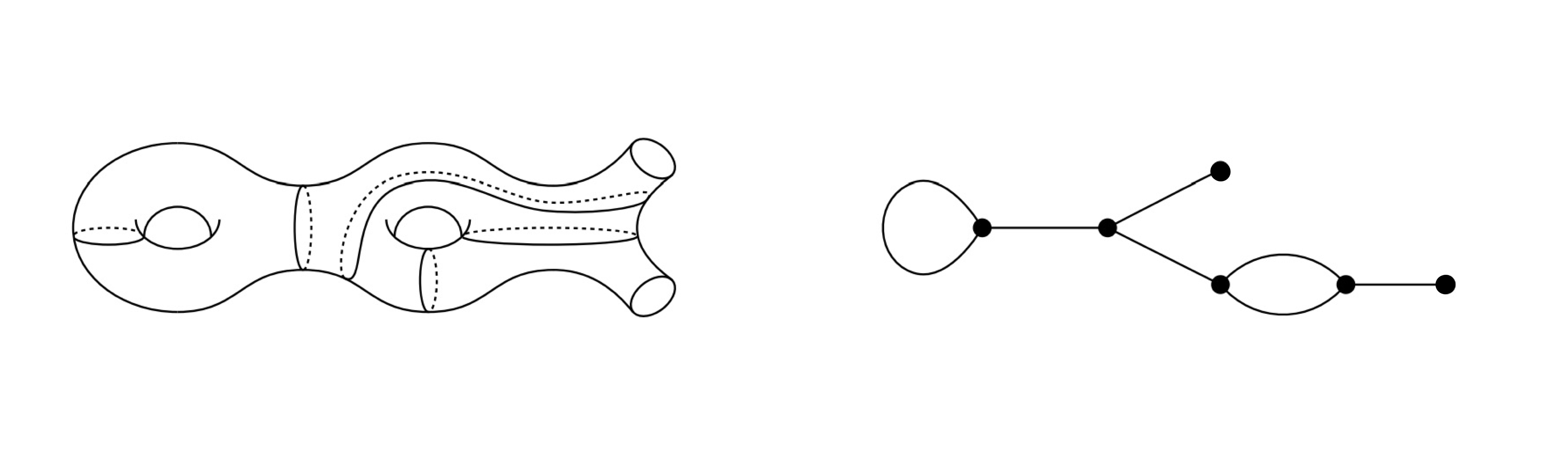
Figure 1: The graph of a pants decomposition of $C_{2,2}$. Figure adapted from Wol (09).

Two pants decompositions $\mf{p}$, $\mf{p}^{\prime}$ are in the same $\mr{MCG}(C_{g,n})$-orbit if and only if the corresponding graphs $G(\mf{p})$, $G(\mf{p}^{\prime})$ are isomorphic Wol (09).

We can now describe the cohomological conditions for the theory defined by the pants decomposition $\mf{p}$ in terms of the graph $G(\mf{p})$ as follows: we begin by labeling the vertices and edges in $G(\mf{p})$ as

$$V\big{(}G(\mf{p})\big{)}:=\{t_{1},\ldots,t_{2g-2+n},u_{1},\ldots,u_{n}\}~{},$$ (214)

$$E\big{(}G(\mf{p})\big{)}:=\{e_{1},\ldots,e_{3g-3+n},\widetilde{e}_{1},\ldots,\widetilde{e}_{n}\}~{},$$ (215)

where $t$ and $u$ indicate trivalent and univalent vertices respectively, whereas the edge $e_{\alpha}$ connects two trivalent vertices and $\widetilde{e}_{i}$ connects a univalent vertex with a trivalent vertex.

In section 9.1, we encountered maps $c_{i}\mapsto c_{1}(c_{i})\in H^{2}({\mathbb{X}},{\mathbb{Z}})$ and $c_{\alpha}\mapsto\mu(b)_{c_{\alpha}}\in H^{2}({\mathbb{X}},{\mathbb{Z}}_{2})$. By design, the set of external cutting curves $\{c_{i}\}_{i=1}^{n}$ is bijectively mapped to the subset $\{\widetilde{e}_{i}\}_{i=1}^{n}$ of edges of $G(\mf{p})$. Likewise, the set of internal cutting curves $\{c_{\alpha}\}_{\alpha=1}^{3g-3+n}$ also gets bijectively mapped to the subset $\{e_{\alpha}\}_{\alpha=1}^{3g-3+n}$. Note, however, that in each case, there might be several bijections due to different choices of indexing. We simply pick one, so that we have one-to-one map between elements of the sets $\{c_{i}\}_{i=1}^{n}$ and $\{\widetilde{e}_{j}\}_{j=1}^{n}$, and between elements of the sets $\{c_{\alpha}\}_{\alpha=1}^{3g-3+n}$ and $\{e_{\beta}\}_{\beta=1}^{3g-3+n}$.

Then, with this choice of map, we can associate fluxes to the edges in $G(\mf{p})$:

$$\widetilde{e}_{i} \longmapsto c_{1}(\widetilde{e}_{i})\in H^{2}({\mathbb{X}},{\mathbb{Z}})\quad\,\,\,\,\text{ for }i=1,\ldots,n~{},$$ (216)

$$e_{\alpha} \longmapsto\mu(b)_{e_{\alpha}}\in H^{2}({\mathbb{X}},{\mathbb{Z}}_{2})\quad\text{ for }\alpha=1,\ldots,3g-3+n~{},$$ (217)

with the proviso that $\mu(b)_{e_{\alpha}}=0$ if $e_{\alpha}$ is a loop (i.e., an edge connecting one vertex to itself). Then, the cohomological conditions described in the preceding section can be recast into equations at each trivalent vertex. If a trivalent vertex is connected by three edges $e_{\alpha}$, $e_{\beta}$, $e_{\gamma}$ to three other trivalent vertices, then we impose the condition

$$\mu(b)_{e_{\alpha}}+\mu(b)_{e_{\beta}}+\mu(b)_{e_{\gamma}}+w_{2}({\mathbb{X}})=0~{}.$$ (218)

If a trivalent vertex is connected by edges $e_{\alpha},e_{\beta},\widetilde{e}_{i}$ to two trivalent and one univalent vertex, then we have the cohomological condition

$$c_{1}(\widetilde{e}_{i})+\mu(b)_{e_{\alpha}}+\mu(b)_{e_{\beta}}+w_{2}({\mathbb{X}})=0\mathsf{\,mod\,}2~{}.$$ (219)

Finally, if a trivalent vertex is connected by edges $e_{\alpha}$, $\widetilde{e}_{i}$, $\widetilde{e}_{j}$ to a trivalent and two univalent vertices, then

$$c_{1}(\widetilde{e}_{i})+\mu(b)_{e_{\alpha}}+w_{2}({\mathbb{X}})=0\mathsf{\,mod\,}2~{},$$ (220)

$$c_{1}(\widetilde{e}_{j})+\mu(b)_{e_{\alpha}}+w_{2}({\mathbb{X}})=0\mathsf{\,mod\,}2~{}.$$ (221)

Now consider two pants decompositions $\mf{p}$, $\mf{p}^{\prime}$ with graphs $G(\mf{p})$, $G(\mf{p}^{\prime})$ in the same $\mr{MCG}(\Sigma_{g,n})$-orbit. Let the vertices and edges of $G(\mf{p}^{\prime})$ be labeled as

$$V\big{(}G(\mf{p}^{\prime})\big{)}:=\{t^{\prime}_{1},\ldots,t^{\prime}_{2g-2+n},u^{\prime}_{1},\ldots,u^{\prime}_{n}\}~{},$$ (222)

$$E\big{(}G(\mf{p}^{\prime})\big{)}:=\{e^{\prime}_{1},\ldots,e^{\prime}_{3g-3+n},\widetilde{e}^{\prime}_{1},\ldots,\widetilde{e}^{\prime}_{n}\}~{}.$$ (223)

We associate fluxes to the edges as in (216) and (217).

Recall that for an undirected graph $G(\mf{p})$, its line graph $L(G(\mf{p}))$ is constructed in the following way: to each edge in $G(\mf{p})$, we assign a vertex in $L(G(\mf{p}))$ and for every two edges in $G(\mf{p})$ emanating from a common vertex, we assign an edge between their corresponding vertices in $L(G(\mf{p}))$. Since $G(\mf{p})\cong G(\mf{p}^{\prime})$, by the Whitney graph isomorphism theorem (Har, 69, Theorem 8.3), their line graphs are also isomorphic:

$$L(G(\mf{p}))\cong L(G(\mf{p}^{\prime}))~{}.$$ (224)

Moreover, there is a one-to-one correspondence between graph isomorphisms $G(\mf{p})\cong G(\mf{p}^{\prime})$ and the corresponding line graph isomorphisms $L(G(\mf{p}))\cong L(G(\mf{p}^{\prime}))$. The vertices of the graphs $L(G(\mf{p}))$ and $L(G(\mf{p}^{\prime}))$ are respectively, $E\big{(}G(\mf{p})\big{)}$ and $E\big{(}G(\mf{p}^{\prime})\big{)}$. Choose an isomorphism $\bm{F}:E\big{(}G(\mf{p})\big{)}\to E\big{(}G(\mf{p}^{\prime})\big{)}$ and let $f:G(\mf{p})\to G(\mf{p}^{\prime})$ denote the graph isomorphism corresponding to $\bm{F}$.

Let us denote an edge in $G(\mf{p})$ connecting two vertices $u$ and $v$ by $uv$. By arguments outlined in (Har, 69, Theorem 8.3), we have

$$\bm{F}(uv)=f(u)f(v)~{}.$$ (225)

In particular, if $e_{\alpha}$, $e_{\beta}$, and $e_{\gamma}$ are edges in $G(\mf{p})$ connecting a vertex $u$ to three other trivalent vertices, then $\bm{F}(e_{\alpha})$, $\bm{F}(e_{\beta})$, $\bm{F}(e_{\gamma})$ are three edges in $G(\mf{p}^{\prime})$ connecting $f(u)$ to three other trivalent vertices in $G(\mf{p}^{\prime})$. Thus by (218), the cohomological condition at the trivalent vertex $f(u)$ in $G(\mf{p}^{\prime})$ is

$$\mu(b^{\prime})_{\bm{F}(e_{\alpha})}+\mu(b^{\prime})_{\bm{F}(e_{\beta})}+\mu(b^{\prime})_{\bm{F}(e_{\gamma})}+w_{2}({\mathbb{X}})=0~{},$$ (226)

where $b^{\prime}$ is the gerbe for the theory defined by the pants decomposition $\mf{p}^{\prime}$. Arguing along the same lines, we conclude that the cohomological conditions for the theory defined by $\mf{p}^{\prime}$ are given by applying the map

$$\widetilde{e}_{i}\longmapsto\bm{F}(\widetilde{e}_{i})~{},\quad e_{\alpha}\longmapsto\bm{F}(e_{\alpha})~{},$$ (227)

to (218), (219), (220) and (221). Thus, we see that at least in this class of examples, $S$-dual theories with different Lagrangians require precisely the same cohomological conditions as needed for the existence of $P^{\mr{phys}}$.

We emphasize that in general the cohomological conditions for two Lagrangian theories which are not in the same S-duality orbit are different and not related by a nice transformation. Consider, for example, the $\mr{a}_{1}$ class ${\cal S}$ theory on a 3 punctured torus $C_{1,3}$. Consider the two pants decompositions of $C_{1,3}$ shown in Figure 2 below.

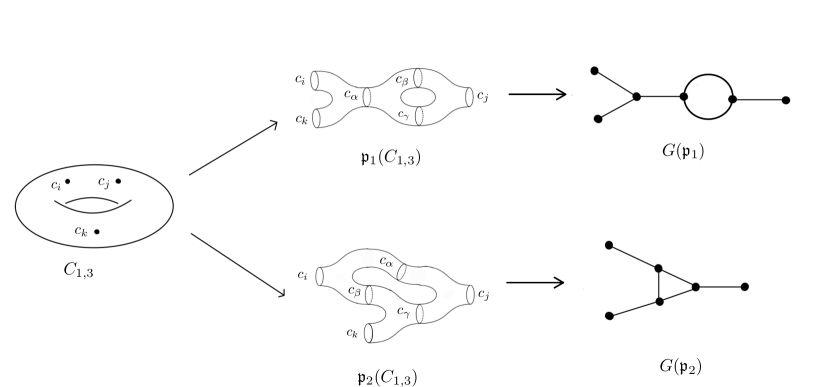
Figure 2: Two $\mr{MCG}(C_{1,3})$-inequivalent pants decompositions of $C_{1,3}$ and their associated pants graphs.

The pants graphs are non-isomorphic as can be easily checked using their adjacency matrix and hence their corresponding Lagrangian theories are not related by $S$-duality. Let us now look at the cohomological conditions we get for the two theories using the general prescription described above. There are three pairs of pants in both pants decompositions. With the labeling of cutting curves in Figure 2, we obtain the following cohomological conditions for the two theories:

1. For the pants decomposition $\mf{p}_{1}(C_{1,3})$ we get

   $$c_{1}(c_{i})+\mu(b)_{c_{\alpha}}+w_{2}({\mathbb{X}}) =0\mathsf{\,mod\,}2~{},$$ (228)

   $$c_{1}(c_{k})+\mu(b)_{c_{\alpha}}+w_{2}({\mathbb{X}}) =0\mathsf{\,mod\,}2~{},$$

   $$\mu(b)_{c_{\alpha}}+\mu(b)_{c_{\beta}}+\mu(b)_{c_{\gamma}}+w_{2}({\mathbb{X}}) =0\mathsf{\,mod\,}2~{},$$

   $$c_{1}(c_{j})+\mu(b)_{c_{\beta}}+\mu(b)_{c_{\gamma}}+w_{2}({\mathbb{X}}) =0\mathsf{\,mod\,}2~{}.$$

2. For the pants decomposition $\mf{p}_{2}(C_{1,3})$ we get

   $$c_{1}(c_{i})+\mu(b)_{c_{\alpha}}+\mu(b)_{c_{\beta}}+w_{2}({\mathbb{X}})=0\mathsf{\,mod\,}2~{},$$ (229)

   $$c_{1}(c_{k})+\mu(b)_{c_{\beta}}+\mu(b)_{c_{\gamma}}+w_{2}({\mathbb{X}})=0\mathsf{\,mod\,}2~{},$$

   $$c_{1}(c_{j})+\mu(b)_{c_{\alpha}}+\mu(b)_{c_{\gamma}}+w_{2}({\mathbb{X}})=0\mathsf{\,mod\,}2~{}.$$

We see that in the second case, we have no restriction on background gerbes since we can always choose a suitable $c_{1}(c_{i,j,k})$ while in the first case, the background gerbes are restricted. Thus the cohomological conditions for the two theories are different.

To twist these theories, we need to provide $C^{\mr{tw}}$ and a homomorphism $\varphi^{\mr{tw}}:G^{\mr{tw}}\to G^{\mr{phys}}$ satisfying (18). Since these theories are Lagrangian, we simply choose $C^{\mr{tw}}$ as in (97) above, and define

$$\varphi^{\mr{tw}}:G^{\mr{tw}} \longrightarrow G^{\mr{phys}}$$ (230)

$${\left[\left(\left(u_{1},u_{2}\right),\mu,g\right)\right]} \longmapsto\left[\left(\left(u_{1},u_{2}\right),u_{2},\mu,g\right)\right].$$

The theories in different $S$-duality orbits correspond to different topological field theories.

Appendix A Symbol Lists

$\mu,\nu,\rho,\ldots$	coordinate indices for a local chart of ${\mathbb{X}}$ (a.k.a. curved spacetime indices) range: $\{1,2,3,4\}$
$\underline{a},\underline{b},\ldots$	indices for a local frame of ${\mathbb{X}}$ (a.k.a. flat indices or frame indices) range: $\{1,2,3,4\}$
$p,q,r,\ldots$	indices labeling a good Čech cover of ${\mathbb{X}}$
$a,b,\ldots$	adjoint-valued indices for $\mr{Lie}(G^{\mr{gauge}})$
$\alpha,\beta,\ldots$	doublet indices of $\mathfrak{su(2)}_{+}$ (a.k.a. undotted spinor indices) range: $\{1,2\}$ Exceptions: Secs. 9.1, 9.2, App. G where they label internal cutting curves.
$\accentset{\mbox{\large.}}{\alpha},\accentset{\mbox{\large.}}{\beta},\ldots$	doublet indices of $\mathfrak{su(2)}_{-}$ (a.k.a. dotted spinor indices) range: $\{1,2\}$
$A,B,\ldots$	doublet indices of $\mf{su(2)}_{\mr{R}}$ (a.k.a. $\mathsf{R}$-symmetry indices) range: $\{1,2\}$
$i,j,\ldots$	multipurpose integer-valued indices Exceptions: Secs. 9.1, 9.2, App. G where they label external cutting curves.
$u,v,\ldots$	flavor indices for hypermultiplets
$m,n,\ldots$	matrix indices for representations of Lie algebra elements

Table A.1: Conventions for indices.

Symbol	Description	Reference
$\alpha$	an element of $C^{\mr{phys}}$	Sec. 4
$\bm{a}$	an element of ${\mathbb{T}}(\mr{SU(N)})$	Sec. 8
$a_{i}$	the $i^{th}$ element of $\bm{a}$	Sec. 8
$\mathsf{adj}$	adjoint representation of a Lie group or algebra	Sec. 7
$A_{\mu}$	connection on $\mathsf{ad\,}P$ in a local chart	Sec. 2
${\cal A}_{\mu}^{u}$	connection on $\mathsf{ad\,}P^{\mr{f},u}$ in a local chart a $\mr{U(1)}/p_{3,u}(C^{\mr{phys}})$ connection	Sec. 7
$A_{\mu}^{\mr{R}}$	a background $\mr{SU(2)_{R}}$ $\mr{R}$-symmetry connection	Sec. 8
$A_{\mu}^{\mr{SU(N)}}$	a background $\mr{SU(N)}$ (flavor) connection	App. F
$A_{\mu}^{\mr{U(1)}}$	a background $\mr{U(1)}$ (flavor) connection	App. F
$\{a_{i}\}$	fugacities for global symmetries	App. E
$A_{1},A_{2}$ $\bar{A}_{1},\bar{A}_{2}$	short multiplets of the $d=4$ ${\cal N}=2$ superconformal algebra	App. D Tables D.1, D.2
${\cal A}^{\Delta}_{R,r(j_{1},j_{2})}$	a two-sided multiplet of the $d=4$ ${\cal N}=2$ superconformal algebra	App. D Eqn. (320)
$\beta$	inverse temperature (for a supersymmetric index)	App. E
$B_{1},\overline{B}_{1}$	short multiplets of the $d=4$ ${\cal N}=2$ superconformal algebra	App. D Table D.1
${\cal B}_{R,r(0,j_{2})}$	a two-sided multiplet of the $d=4$ ${\cal N}=2$ superconformal algebra	App. D Eqn. (320)
$\widehat{{\cal B}}_{R}$	a two-sided multiplet of the $d=4$ ${\cal N}=2$ superconformal algebra	App. D Eqn. (320)
$B_{\mu}^{u}$	a $\mr{U(1)}_{u}$ connection	Sec. 7 Eqn. (115)
$b$	a flat $C^{\mr{grb}}$-gerbe connection (background field)	Sec. 3
$\bm{b}$	an element of ${\mathbb{T}}(\mr{SU(N)})$	Sec. 8
$b_{i}$	the $i^{th}$ element of $\bm{b}$	Sec. 8
$\mr{Bord}_{\leq 4}^{\mathfrak{F}}$	bordism category of manifolds of dimension $\leq 4$ equipped with background fields $\mathfrak{F}$	Sec. 2
$\bm{c}$	an element of ${\mathbb{T}}(\mr{SU(N)})$	Sec. 8
$c_{1}(\mr{f})$	first Chern class of a $\mr{U(1)}$ bundle obtained from $P^{\mr{f}}$	Sec. 4
$c_{1}(u)$	first Chern class of a $\mr{U(1)}$ bundle obtained from $P^{\mr{f},u}$	Secs. 4, 7 Eqn. (129)
$c_{1}(\widetilde{e}_{i})$	first Chern class of a $\mr{U(1)}$ bundle associated to an edge $\widetilde{e}_{i}\in E\big{(}G(\mf{p})\big{)}$	Sec. 9.2 Eqn. (216)
$c_{1}(c_{i}^{\mr{s}})$	first Chern class of a $\mr{U(1)}$ bundle obtained from $P^{f,c_{i}^{\mr{s}}}$	App. 9.2
$c$	element of the group $C$	Sec. 2
$c_{i}$	external cutting curve for a pants decomposition	Sec. 8, App. G
$c_{\alpha}$	internal cutting curve for a pants decomposition	Sec. 8, App. G
$c_{i}^{\mr{f}}$	external cutting curve bounding a full puncture	App. G
$c_{i}^{\mr{s}}$	external cutting curve bounding a simple puncture	App. G
$c_{T,i}$	external cutting curve bounding a trinion $T$	App. G
$c_{T,\alpha}$	internal cutting curve bounding a trinion $T$	App. G
${\cal C}$	conformal manifold	Sec. 1
$C^{(1)},C^{(2)}$	stable Riemann surfaces	Sec. 8
$C$	subgroup of $Z(\widetilde{G})$	Sec. 2
$C^{\mr{bck}}$	subgroup of $Z(\mr{Spin(4)}\times\mr{SU(2)_{R}}\times G^{\mr{f}})$	Sec. 5 Eqn. (81)
$C^{\mr{grb}}$	subroup of $Z(\widetilde{G}^{\mr{gauge}})$ defined to be $p_{4}(C^{\mr{phys}})$	Sec. 3 Eqn. (32)
$C^{\mr{phys}}$	a subgroup of $Z(\widetilde{G}^{\mr{phys}})$	Sec. 3
$C^{\mr{phys}}_{\mr{max}}$	the maximal choice of $C^{\mr{phys}}$	Sec. 3 Eqn. (31)
$C^{\mr{tw}}$	subgroup of $Z(\mr{Spin(4)}\times{\mathbb{T}}^{\mr{f}}\times\widetilde{G}^{\mr{gauge}})$	Sec. 5 Eqn. (82)
$C_{1}^{\mr{tw}}$	a subgroup of $Z(\widetilde{G}_{1}^{\mr{tw}})$	Sec. 6 Eqn. (101)
$C_{2}^{\mr{tw}}$	a subgroup of $Z(\widetilde{G}_{2}^{\mr{tw}})$	Sec. 6 Eqn. (104)
$C_{3}^{\mr{tw}}$	a subgroup of $Z(\widetilde{G}_{3}^{\mr{tw}})$	Sec. 6 Eqn. (107)
$C_{g,n}$	ultraviolet curve	Sec. 8
$C_{T}$	subgroup of $Z(\widetilde{G}_{T})$	Sec. 8
$C_{T}^{\mr{max}}$	the maximal choice of $C_{T}$	Sec. 8
$C_{{\cal T}}$	subgroup of $Z(\widetilde{G}_{{\cal T}})$	Sec. 8
$C_{{\cal T}}^{\mr{max}}$	maximal choice of $C_{{\cal T}}$	Sec. 8 Eqn. (193)
$C_{{\cal T}}^{\prime}$	specific subgroup of $Z(\widetilde{G}_{{\cal T}})$	Sec. 8 Eqn. (196)
$C_{{\cal T}}^{\prime\prime}$	preimage of $C_{{\cal T}}^{\prime}$ under the product over $\alpha$ of the map $\Delta:\mr{SU(N)}\to\Delta(\mr{SU(N)})$	Sec. 8
$C_{\mr{S}}^{\mr{tw}}$	$C^{\mr{tw}}$ for a twisted class ${\cal S}$ theory $\mr{S}$	Sec. 8
${\cal C}_{R,r(j_{1},j_{2})}$	a two-sided multiplet of the $d=4$ ${\cal N}=2$ superconformal algebra	App. D Eqn. (320)
$\widehat{{\cal C}}_{R(j_{1},j_{2})}$	a two-sided multiplet of the $d=4$ ${\cal N}=2$ superconformal algebra	App. D Eqn. (320)
$C_{c_{i}^{\mr{f}}}$	the group $p_{3,c_{i}^{\mr{f}}}(C^{\prime\prime}_{{\cal T}})$	App. G Eqn. (363)
$C_{c_{\alpha}}$	the group $p_{4,c_{\alpha}}(C^{\prime\prime}_{{\cal T}})$	App. G Eqn. (363)
$\chi_{\mu\nu}$	SD 2-form gaugino	Sec. 7
$\chi^{\alpha,\overline{n}m}$	complex conjugate of $\psi_{\alpha,m\overline{n}}$	App. F Eqn. (332)
$\widetilde{\chi}_{\accentset{\mbox{\large.}}{\alpha},m\overline{n}}$	Weyl spinor in $\widetilde{Q}^{\prime m\overline{n}}$	App. F Eqn. (329)
$\chi_{\lambda}$	character of the representation $\lambda$	Sec. 8
$D_{p_{i}}$	data at the $i^{th}$ puncture of a trinion theory ($i=1,2,3$)	Sec. 8
$\not{D}_{E}^{\pm}$	chiral Dirac operator coupled to a vector bundle $E$	Sec. 2, App. F Eqn. (339)
$D_{\mu}$	covariant derivative	Sec. 7
$D_{{\cal V}\otimes\overline{{\cal V}}}$	spinor covariant derivatives	App. F Eqns. (337), (338)
$\not{D}^{\pm}_{{\cal V}\otimes\overline{{\cal V}}}$	chiral Dirac operators coupled to ${\cal V}\otimes\overline{{\cal V}}$	App. F Eqn. (341)
$\Delta$	dilatation generator or conformal dimension	Sec. 8
$\Delta(G)$	diagonal subgroup of $G\times G$	Sec. 8
$D_{\mu\nu}$	SD 2-form auxiliary field of the twisted VM	Sec. 7
$D_{\accentset{\mbox{\large.}}{\alpha}\accentset{\mbox{\large.}}{\beta}}$	SD auxiliary field $D_{\mu\nu}$ in spinor notation	Sec. 7
$D_{AB}$	auxiliary field in the untwisted $d=4$ ${\cal N}=2$ VM	App. F
$\mathscr{D}$	auxiliary field in the background ${\cal N}=2$ conformal supergravity multiplet	App. F
$\mathsf{DET}$	determinant line bundle of a chiral Dirac operator	App. F
$\mathsf{Det}$	a section of $\mathsf{DET}$	App. F
$[{\cal D}\mr{HM}]$	path integral measure for a $d=4$ ${\cal N}=2$ hypermultiplet	Sec. 8
${\cal D}_{R(0,j_{2})}$	a two-sided multiplet of the $d=4$ ${\cal N}=2$ superconformal algebra	App. D Eqn. (320)
$e_{\mu}{}^{\underline{a}}$	vielbein in a local chart	Sec. 7
$\{e_{i}\}_{i=1}^{3g-3+n}$	edge in $G(\mf{p})$ connecting two trivalent vertices	Sec. 9.2
$\{\widetilde{e}_{i}\}_{i=1}^{n}$	edge in $G(\mf{p})$ connecting a univalent vertex with a trivalent vertex	Sec. 9.2
$E$	a complex vector bundle	App. F
$E_{\rho}$	vector bundle associated to $P^{\mr{phys}}$	Sec. 3
$E^{\mr{tw}}$	vector bundle associated to $P^{\mr{tw}}$	Sec. 5
$E^{\mr{mon}}$	vector bundle associated to $G^{\mr{tw}}$-bundle	Sec. 7
$E\big{(}G(\mf{p})\big{)}$	list of edges in $G(\mf{p})$	Sec. 9.2 Eqn. (215)
$\eta^{\mr{f}}_{pqr}$	Čech 2-cocycle representative of $c_{1}({\mr{f}})$	Sec. 4 Eqn. (59)
$\eta$	0-form gaugino	Sec. 7
${\cal E}_{r(0,j_{2})}$	a two-sided multiplet of the $d=4$ ${\cal N}=2$ superconformal algebra	App. D Eqn. (320)
$\varepsilon_{pq}r$	coboundary from $U_{pq}$ to some finite cyclic group	App. C
$\varepsilon_{pq}$	cochain that trivializes $\varepsilon_{pqr}$	App. C
$\{f_{i}\}$	conserved flavor charges	App. E
$\mr{F}$	fermion number operator	Sec. 8, App. E
$F$	curvature of $A_{\mu}$	Sec. 7
$F^{u}$	curvature of $B_{\mu}^{u}$	Sec. 7
$F_{\accentset{\mbox{\large.}}{\alpha}\accentset{\mbox{\large.}}{\beta}}$	self-dual part of $F_{\mu\nu}^{+}$ in spinor notation	Sec. 7
${\cal F}^{\mr{bck}}$	background fields for a quantum theory	Sec. 5 Eqns. (77), (79)
${\cal F}^{\mr{phys}}$	background fields for a bordism category	Sec. 3 Eqn. (35)
${\cal F}^{{\cal Q}}$	${\cal Q}$-invariant background parameters	Sec. 1
${\cal F}^{\mr{tw}}$	fields of the twisted theory	Sec. 5 Eqn. (83)
${\cal F}^{\mr{tw},\mr{bck}}$	background fields of the twisted theory	Sec. 5 Eqn. (87)
$\mathfrak{F}$	a set (or more precisely, sheaf) of background fields	Sec. 2
$\widetilde{\mathcal{F}}$	background fields for a $d=4$ ${\cal N}=2$ field theory	Sec. 2
$\mathsf{Fr}({\mathbb{X}})$	Frame bundle of ${\mathbb{X}}$ derived from $P^{\mr{phys}}$	Sec. 3 Eqn. (28)
$F^{u}$	curvature of background $\mr{U(1)}_{u}$ connection	Sec. 7
$\bm{F}$	an isomorphism $E\big{(}G(\mf{p})\big{)}\to E\big{(}G(\mf{p}^{\prime})\big{)}$	Sec. 9.2
$f$	a graph isomorphism $G(\mf{p})\to G(\mf{p}^{\prime})$	Sec. 9.2
$\varphi$	a homomorphism $\widetilde{G}^{\mr{phys}}\to\widetilde{G}^{\mr{phys}}$	Sec. 5 Eqn. (94)
$\overline{\varphi}$	a homomorphism $G^{\mr{tw}}\to G^{\mr{phys}}$	Sec. 5 Eqn. (98)
$\varphi^{\mr{W}}$	the Witten homomorphism	Sec. 2 Eqns. (12), (14)
$\varphi^{\mr{tw}}$	a twisting homomorphism $G^{\mr{tw}}\to G^{\mr{phys}}$	Sec. 5
$\varphi^{\mr{tw,bck}}$	a homomorphism for twisted background field data	Sec. 2 Eqn. (15)
$\widetilde{\varphi}^{\mr{tw,bck}}$	a homomorphism for twisted background field data	Sec. 2 Eqn. (16)
$\varphi_{\rho}^{G}$	a homomorphism $H\to{\mathbb{T}}^{\mr{f}}$	Sec. 6 Eqn. (88)
$\varphi_{1}^{\mr{GL}}$	twisting homomorphism for the GL Twist of ${\cal N}=4$ SYM	Sec. 6 Eqn. (102)
$\overline{\varphi}_{1}^{\mr{GL}}$	twisting homomorphism for the GL Twist of ${\cal N}=4$ SYM	Sec. 6 Eqn. (103)
$\varphi_{2}^{\mr{DW}}$	twisting homomorphism for the DW Twist of ${\cal N}=4$ SYM	Sec. 6 Eqn. (105)
$\overline{\varphi}_{2}^{\mr{DW}}$	twisting homomorphism for the DW Twist of ${\cal N}=4$ SYM	Sec. 6 Eqn. (106)
$\varphi_{3}^{\mr{VW}}$	twisting homomorphism for the VW Twist of ${\cal N}=4$ SYM	Sec. 6 Eqn. (109)
$\overline{\varphi}_{3}^{\mr{VW}}$	twisting homomorphism for the VW Twist of ${\cal N}=4$ SYM	Sec. 6 Eqn. (110)
$\widetilde{\varphi}^{\mr{tw}}$	twisting homomorphism for a class ${\cal S}$ theory	Sec. 6 Eqn. (204)
$\phi$	${\cal N}=2$ vectormultiplet scalar	Sec. 7
$\widetilde{\phi}$	${\cal N}=2$ vectormultiplet scalar	Sec. 7
$\phi_{u}$	a scalar in the ${\mathbb{T}}^{\mr{f}}$ vectormultiplet	Sec. 7 Eqn. (116)
$\widetilde{\phi}_{u}$	a scalar in the ${\mathbb{T}}^{\mr{f}}$ vectormultiplet	Sec. 7 Eqn. (116)
$\Phi^{\mr{grav}}$	gravitational background fields	Sec. 3
$\Phi^{\mr{phys}}$	physical fields	Sec. 3
$\Phi^{\mr{tw}}$	a section of $E^{\mr{tw}}$	Sec. 5 Eqn. (83)
$\Phi_{c_{1},c_{2},c_{3}}$	half-hypermultiplet trinion in the $\mf{a}_{1}$ class ${\cal S}$ theory	Sec. 9
$\psi^{\mr{tw}}$	homomorphism $H\to Z(\widetilde{G}^{\mr{tw}})$	Sec. 5 Eqn. (95)
$\psi_{\mu}$	1-form gaugino	Sec. 7
$\psi_{\mr{glue}}$	gluing homomomorphisms for gauging the diagonal flavor symmetry	Sec. 8 Eqns. (194), (195)
$\psi_{\alpha}^{m\overline{n}}$	Weyl spinor in $Q^{m\overline{n}}$	App. F Eqn. (329)
$\widetilde{\psi}^{\accentset{\mbox{\large.}}{\alpha},\overline{n}m}$	complex conjugate of $\psi_{\alpha,m\overline{n}}$	App. F Eqn. (332)
$\bm{g}$	element of flavor group or flavor fugacity	Sec. 8
$g$	genus of a Riemann surface (UV curve)	Sec. 8
$g_{\mu\nu}$	Riemannian metric on ${\mathbb{X}}$ in local coordinates	Sec. 2
$\mathfrak{g}$	Lie algebra of a Lie group	Sec. 8
$\mathfrak{g}_{p}^{\mr{fl}}$	flavor Lie algebra associated to puncture $p$	Sec. 8
$\widetilde{G}$	global symmetry group	Sec. 2 Eqn. (4)
$G^{\mr{bck}}$	structure group of background bundle $P^{\mr{bck}}$	Sec. 5 Eqn. (81)
$G^{\mr{f}}$	flavor group	Sec. 2
$G_{f}^{\pm}$	the group $\mr{SU(N)}\times\mr{SU(N)}\times\mr{U(1)}$	App. F.2 Eqn. (352)
$G^{\mr{gauge}}$	compact, connected, semisimple Lie group (“gauge group”) given by the quotient group $\widetilde{G}^{\mr{gauge}}/C^{\mr{grb}}$	Sec. 3
$\widetilde{G}^{\mr{gauge}}$	simply-connected cover of $G^{\mr{gauge}}$	Sec. 3
$G^{\mr{phys}}$	structure group of a Lagrangian $d=4$ ${\cal N}=2$ theory given as the quotient group $\widetilde{G}^{\mr{phys}}/C^{\mr{phys}}$	Sec. 3
$\widetilde{G}^{\mr{tw}}$	the group $\mr{Spin(4)}\times{\mathbb{T}}^{\mr{f}}\times\widetilde{G}^{\mr{gauge}}$ the simply-connected cover of $G^{\mr{tw}}$	Secs. 5, 6 Eqn. (93)
$G^{\mr{tw}}$	the group $\widetilde{G}^{\mr{tw}}/C^{\mr{tw}}$ the structure group of a topologically-twisted theory	Secs. 5, 6 Eqn. (82)
$G^{\mr{tw},\mr{bck}}$	structure group of $P^{\mr{tw},\mr{bck}}$	Sec. 5 Eqn. (86)
$\widetilde{G}_{1}^{\mr{tw}}$	the group $\mr{Spin(4)}\times\mr{U(1)_{R}}\times\widetilde{G}^{\mr{gauge}}$	Sec. 6 Eqn. (101)
$G_{1}^{\mr{tw}}$	structure group for the GL twist of ${\cal N}=4$ SYM given as a quotient group $\widetilde{G}_{1}^{\mr{tw}}/C_{1}^{\mr{tw}}$	Sec. 6 Eqn. (101)
$\widetilde{G}_{2}^{\mr{tw}}$	the group $\mr{Spin(4)}\times\mr{U(2)_{R}}\times\widetilde{G}^{\mr{gauge}}$	Sec. 6 Eqn. (104)
$G_{2}^{\mr{tw}}$	structure group for the DW twist of ${\cal N}=4$ SYM given as a quotient group $\widetilde{G}_{2}^{\mr{tw}}/C_{2}^{\mr{tw}}$	Sec. 6 Eqn. (104)
$\widetilde{G}_{3}^{\mr{tw}}$	the group $\mr{Spin(4)}\times\mr{SU(2)_{R}}\times\widetilde{G}^{\mr{gauge}}$	Sec. 6 Eqn. (107)
$G_{3}^{\mr{tw}}$	structure group for the VW twist of ${\cal N}=4$ SYM given as a quotient group $\widetilde{G}_{3}^{\mr{tw}}/C_{3}^{\mr{tw}}$	Sec. 6 Eqn. (107)
$\widetilde{G}_{p}$	simply-connected cover of the flavor symmetry at puncture $p$	Sec. 8
$G_{T}$	global symmetry group of the trinion theory $T$	Sec. 8 Eqn. (155)
$\widetilde{G}_{T}$	simply-connected cover of $G_{T}$	Sec. 8 Eqn. (152)
$\widetilde{G}_{{\cal T}}$	simply-connected cover of the global symmetry of a product of trinions	Sec. 8 Eqn. (191)
$\widetilde{G}_{\mr{S}}$	$\widetilde{G}^{\mr{phys}}$ for a class ${\cal S}$ theory	Sec. 8 Eqn. (198)
$G_{\mr{S}}$	$G^{\mr{phys}}$ for an $A_{N-1}$ class ${\cal S}$ theory	App. G Eqn. (359)
$G(\mf{p})$	graph of a pants decomposition $\mf{p}$	Sec. 9.2
$G_{T}^{\mr{extended}}$	the group $\mr{Spin(4)}\times\mr{SU(2)_{R}}\times G_{f}^{+}\times G_{f}^{-}$	App. F.2 Eqn. (353)
$\widetilde{G}_{\mu\accentset{\mbox{\large.}}{\alpha}}^{A}$	component of supercurrent in a local $d=4$ ${\cal N}=2$ theory	Sec. 2, App. D
$G_{\mu{\alpha}}^{A}$	component of supercurrent in a local $d=4$ ${\cal N}=2$ theory	Sec. 2, App. D
$\widetilde{G}_{c_{i}}$	simply connected cover of the flavor group at an external cutting curve $c_{i}$	App. G
$H$	the group $p_{4}(C^{\mr{phys}})\times{\mathbb{Z}}_{2}$	Sec. 6
${\cal H}$	the Hilbert space of a supersymmetric theory	App. E
$h_{\alpha}$	auxiliary Weyl fermion in the twisted ${\cal N}=2$ hypermultiplet	Sec. 7 Table 4
$\widetilde{h}_{\alpha}$	auxiliary Weyl fermion in the twisted ${\cal N}=2$ hypermultiplet	Sec. 7 Table 4
$h_{\alpha}^{u}$	auxiliary Weyl fermion for the $u^{th}$ multiplet	Sec. 7
$\widetilde{h}_{\alpha}^{u}$	auxiliary Weyl fermion for the $u^{th}$ multiplet	Sec. 7
${{\cal I}}(p,q,t;\{a_{i}\})$	the ${\cal N}=2$ superconformal index	Sec. E Eqn. (E)
${{\cal I}}_{\mr{Schur}}(q,\bm{g})$	the Schur index of a $d=4$ ${\cal N}=2$ SCFT	Sec. 8, App. E Eqns. (158), (328)
${{\cal I}}_{\mr{Schur}}(q,\bm{a},\bm{b},\alpha)$	the Schur index of the $\mr{ffs}$ trinion theory	Sec. 8 Eqn. (163)
${{\cal I}}_{\mr{Schur}}(q,\bm{a},\bm{b},\bm{c})$	the Schur index of the $T_{N}$ ($\mr{fff}$) trinion theory	Sec. 8 Eqn. (172)
$j_{1},j_{2}$	Cartan generators of $\mr{SU(2)}_{1}\times\mr{SU(2)}_{2}$ ${\mathbb{Z}}$-valued eigenvalues of the Cartan generators	Sec. 8 App. E
$J^{a}_{\mu}$	conserved flavor current	Sec. 2, App. D
$k_{1},k_{2},k_{3}$	integers in $\{0,\ldots,N-1\}$	Sec. 8
$k_{1}^{\pm},k_{2}^{\pm}$	integers in $\{0,\ldots,N-1\}$	App. F.2
$K(\bm{a})$	a $(q,\bm{a})$-dependent function entering the Schur index	Sec. 8 Eqn. (175)
$K_{0}$	a $(q,N)$-dependent function entering the Schur index	Sec. 8 Eqn. (176)
$K$	kernel of $\pi\circ\psi_{\mr{glue}}$	Sec. 8
$L,\bar{L}$	short multiplets of the $d=4$ ${\cal N}=2$ superconformal algebra	App. D Tables D.1, D.2
$\mr{\Lambda}^{\mr{max}}$	top exterior power	App. F
${\cal L}$	extra data needed to make a relative theory absolute	Sec. 8
$L\big{(}G(\mf{p})\big{)}$	line graph of a graph $G(\mf{p})$	Sec. 9.2
$\Lambda$	dynamical scale (a background field)	Sec. 5
$\Lambda_{\mu\nu}$	twisted supercurrent of a topological $d=4$ ${\cal N}=2$ theory	Sec. 2
$\lambda_{\alpha}$	Weyl fermion in the twisted ${\cal N}=2$ hypermultiplet	Sec. 7 Table 4
$\lambda^{\alpha u}$	$\lambda^{\alpha}$ field for the $u^{th}$ multiplet	Sec. 7
$\widetilde{\lambda}_{\accentset{\mbox{\large.}}{\alpha}}$	Weyl fermion in the twisted ${\cal N}=2$ hypermultiplet	Sec. 7 Table 4
$\widetilde{\lambda}^{\accentset{\mbox{\large.}}{\alpha}u}$	$\widetilde{\lambda}^{\accentset{\mbox{\large.}}{\alpha}}$ field for the $u^{th}$ multiplet	Sec. 7
$m$	mass parameters of the theory	Sec. 1
$\mu(b)$	characteristic class of a background flat $C^{\mr{grb}}$-gerbe $b$	Sec. 4 Eqn. (45)
$\mu(b)_{e_{\alpha}}$	characteristic class of a background flat $C^{\mr{grb}}$-gerbe $b$ associated to an edge $\widetilde{e}_{\alpha}\in E\big{(}G(\mf{p})\big{)}$	Secs. 9.2 Eqn. (217)
$\mu(b)_{c_{i}^{\mr{f}}}$	characteristic class of a background flat $C_{c_{i}^{\mr{f}}}$-gerbe $b_{c_{i}^{\mr{f}}}$	Secs. 9.2 Eqn. (364)
$\mu(b)_{c_{\alpha}}$	characteristic class of a background flat $C_{c_{\alpha}}$-gerbe $b_{c_{\alpha}}$	Secs. 9.2 Eqn. (364)
$\mu_{\alpha}$	Weyl fermion in the twisted ${\cal N}=2$ hypermultiplet	Sec. 7 Table 4
$\widetilde{\mu}_{\accentset{\mbox{\large.}}{\alpha}}$	Weyl fermion in the twisted ${\cal N}=2$ hypermultiplet	Sec. 7 Table 4
$\mu^{\alpha u}$	$\mu^{\alpha}$ field for the $u^{th}$ multiplet	Sec. 7
$\widetilde{\mu}^{\accentset{\mbox{\large.}}{\alpha}u}$	$\mu^{\accentset{\mbox{\large.}}{\alpha}}$ field for the $u^{th}$ multiplet	Sec. 7
$\mu$	an element of $Z(\widetilde{G_{p_{1}}}\times\widetilde{G_{p_{2}}}\times\widetilde{G_{p_{3}}})$	Sec. 8
$\mu^{(\!(AB)\!)a}$	bottom component of the flavor multiplet	App. D
$m$	mass parameter	Sec. 7
$M_{\accentset{\mbox{\large.}}{\alpha}}$	monopole field	Sec. 7, App. F Table 4
$\widetilde{M}_{\accentset{\mbox{\large.}}{\alpha}}$	conjugate monopole field	Sec. 7, App. F Table 4
$M^{\accentset{\mbox{\large.}}{\alpha}}_{u}$	monopole field in the $u^{th}$ multiplet	Sec. 7
$\widetilde{M}^{\accentset{\mbox{\large.}}{\alpha}u}$	conjugate monopole field in the $u^{th}$ multiplet	Sec. 7
$\mr{MCG}(C_{g,n})$	mapping class group of $C_{g,n}$	Sec. 9.2
$n$	a context-dependent integer number of punctures or boundary components of $C_{g,n}$	Sec. 8
$n_{u}$	the order of the group $p_{3,u}(C^{\mr{phys}})\cong{\mathbb{Z}}/n_{u}{\mathbb{Z}}$	Sec. 7
$n_{c_{i}^{\mr{s}}}$	the order of the group $p_{3,c_{i}^{\mr{s}}}(C_{{\cal T}}^{\prime\prime})\cong{\mathbb{Z}}/n_{c_{i}^{\mr{s}}}{\mathbb{Z}}$	App. G Eqn. (362)
${\cal N}$	number of independent real supercharges divided by the dimension of the minimal spinor representation	Sec. 1
$\bm{\nabla}$	connection on $P$	Sec. 2
$\widetilde{\bm{\nabla}}$	connection on $\widetilde{P}$	Sec. 2
$\bm{\nabla}^{\mr{phys}}$	connection on $P^{\mr{phys}}$	Sec. 3
$\bm{\nabla}^{\mr{LC}}$	torsion-free connection associated to a Riemannian metric on ${\mathbb{X}}$	Sec. 3
$\bm{\nabla}^{\mr{bck}}$	connection on $P^{\mr{bck}}$	Sec. 5 Eqn. (80)
$\bm{\nabla}^{\mr{tw}}$	connection on $P^{\mr{tw}}$	Sec. 5 Eqn. (83)
$\bm{\nabla}^{\mr{tw},\mr{bck}}$	connection on $P^{\mr{tw},\mr{bck}}$	Sec. 5 Eqn. (87)
$\bm{\nabla}_{T}$	$\widetilde{G}_{T}$-connection on $\widetilde{P}_{T}$	App. F
$\bm{\nabla}_{\mu}^{\mr{f}}$ and $\bm{\nabla}^{\mu}_{\mr{f}}$	(metric + flavor + $\mr{SU(2)_{R}}$)-covariant derivatives	App. F Eqns. (335), (336)
${\cal O}$	the ${\cal Q}$-cohomology of the space of (extended) observables	Sec. 1
$O_{i}$	a basis of the vector space ${\cal O}$	Sec. 1
${\cal O}^{\vee}$	dual space of ${\cal O}$	Sec. 1
$\mr{OFr}({\mathbb{X}})$	bundle of oriented frames over ${\mathbb{X}}$ (a.k.a. frame bundle)	Sec. 2
$\omega_{\mu}{}^{\underline{a}\,\underline{b}}$	spin connection in local coordinates	Sec. 6
$(\omega_{+})_{\mu}$	SD part of spin connection	Sec. 7
$\omega$	primitive $N^{th}$ root of unity equal to $e^{2\pi\mathsf{i}/N}$	Sec. 8
$\varpi$	a map $H^{2}({\mathbb{X}},C^{\mr{grb}})\to H^{2}({\mathbb{X}},{\mathbb{Z}}_{2}^{3g-3+n})$	Sec. 9
$P$	a principal $G$-bundle on ${\mathbb{X}}$	Sec. 2
$\widetilde{P}$	principal $\widetilde{G}$-bundle on ${\mathbb{X}}$	Sec. 2
$P^{\mr{bck}}$	background bundle with connection	Sec. 5 Eqn. (80)
$P^{\mr{f}}$	flavor bundle of $d=4$ ${\cal N}=2$ theory	Sec. 3 Eqn. (28)
$P^{\mr{f},c_{i}}$	a $\mr{U(1)}/p_{3,c_{i}}(C^{\mr{phys}})$-bundle	Sec. 9 Eqn. (210)
$P^{\mr{gauge}}$	gauge bundle of a $d=4$ ${\cal N}=2$ theory	Sec. 3 Eqn. (28)
$P^{\mr{gauge},c_{\alpha}}$	gauge bundle of an $A_{N-1}$ Class ${\cal S}$ theory associated with internal curve $c_{\alpha}$	App. G Eqn. (361)
$P^{\mr{phys}}$	principal $G^{\mr{phys}}$-bundle over ${\mathbb{X}}$	Sec. 3
$P^{\mr{R}}$	$\mr{R}$-symmetry bundle of $d=4$ ${\cal N}=2$ theory	Sec. 3 Eqn. (28)
$P^{\mr{tw}}$	bundle with connection for a twisted theory	Sec. 5 Eqn. (83)
$P_{\mr{S}}$	a principal $G_{\mr{S}}$ bundle on ${\mathbb{X}}$	App. G
$P^{\mr{tw},\mr{bck}}$	background field bundle with connection for a twisted theory	Sec. 5 Eqn. (87)
$P_{T}$	a principal $\widetilde{G}_{T}$-bundle on ${\mathbb{X}}$	Sec. 8, App. F
$p_{i}$	projection onto the $i^{th}$ factor	Sec. 2 Eqn. (5)
$p_{3,c_{i}}$	projection onto $c_{i}^{th}$ gauge factor	App. G Eqn. (360)
$p_{4,c_{\alpha}}$	projection onto $c_{\alpha}^{th}$ flavor factor	App. G Eqn. (360)
$\mf{p}$	list of cutting curves defining a pants decompositon	Sec. 8 Eqn. (151)
$\pi_{{\mathbb{X}}}$	$p_{1}$ precomposed with the homomorphism $\mr{Spin(4)}\to\mr{SO(4)}$	Sec. 2
$\pi$	natural quotient homomorphism $\widetilde{G}\to G$ defines a functor $\pi_{*}:\mr{Bord}_{\leq 4}^{\widetilde{{\cal F}}}\to\mr{Bord}_{\leq 4}^{{\cal F}}$	Sec. 2
$\pi_{\Lambda}$	Fibration ${\cal F}^{\mr{phys}}\to{\cal F}^{\mr{bck}}$ or ${\cal F}^{\mr{tw}}\to{\cal F}^{\mr{tw},\mr{bck}}$	Sec. 5 Eqn. (78), (85)
$\widetilde{\psi}_{\accentset{\mbox{\large.}}{\alpha}}^{Aa}$	${\cal Q}$-superpartner of $J_{\mu}^{a}$	Sec. 2, App. D
$\psi_{\alpha}^{Aa}$	$\widetilde{{\cal Q}}$-superpartner of $J_{\mu}^{a}$	Sec. 2, App. D
$\psi_{\alpha}^{m\overline{n}}$	a Weyl spinor in $Q^{m\overline{n}}$	App. F Eqn. (329)
${\cal Q}$	scalar supercharge	Sec. 1
${\cal Q}_{\alpha A}$	supercharge in a $d=4$ ${\cal N}=2$ theory	Sec. 2
$Q^{m\overline{n}}$	a chiral multiplet in $V\otimes\overline{V}$	App. F Eqn. (329)
$\widetilde{Q}^{\prime m\overline{n}}$	an anti-chiral multiplet in $V\otimes\overline{V}$	App. F Eqn. (329)
$(q^{2})^{m\overline{n}}$	a complex scalar in $Q^{m\overline{n}}$	App. F Eqn. (329)
$(q^{1})^{m\overline{n}}$	a complex scalar in $\widetilde{Q}^{\prime m\overline{n}}$	App. F Eqn. (329)
$(\widetilde{q}^{A})^{\overline{n}m}$	complex conjugate of $q_{A,m\overline{n}}$	App. F Eqn. (330)
$q^{\rho}$	a $(q,N)$-dependent vector in the $\underline{\bm{N}}$ of $\mr{SU(N)}$	Sec. 8 Eqn. (174)
$\rho$	a quaternionic representation on a real vector space ${\cal R}$ a map $\widetilde{G}^{\mr{gauge}}\to\mr{End}_{{\mathbb{R}}}({\cal R})$	Sec. 3
$\varrho$	complex summand of quaternionic representation $\rho$	Sec. 7 Eqn. (111)
$\overline{\varrho}$	complex conjugate representation of $\varrho$	Sec. 7 Eqn. (111)
$r$	Cartan generator of $\mr{U(1)_{R}}$ ${\mathbb{R}}$-valued eigenvalue of the Cartan generator of $\mr{U(1)_{R}}$	Sec. 8, App. E
$R$	Cartan generator of $\mr{SU(2)_{R}}$ ${\mathbb{Z}}$-valued eigenvalue of the Cartan generator of $\mr{SU(2)_{R}}$	Sec. 8, App. E
${\cal R}$	a real vector space ${\cal R}$ equipped with a $G^{\mr{gauge}}$-invt. positive inner product	Sec. 3
$(\rho,{\cal R})$	representation of a hypermultiplet under $\widetilde{G}^{\mr{gauge}}$	Sec. 3
$\mathscr{R}$	Ricci scalar of the 4-manifold ${\mathbb{X}}$	App. F
$\rho_{s}$	a map ${\mathbb{Z}}/2{\mathbb{Z}}\to{\cal Z}_{u}$	Sec. 4
$\rho_{u}$	irreducible components of $\rho$	Sec. 4
$q_{u}$	integer valued charge of hypermultiplet under $\mr{U(1)}_{u}$	Sec. 7
$q,p,t$	superconformal fugacities	Sec. 8 App. E
$r_{n}$	reduction modulo $n$	Sec. 4
$R_{T}(z)$	a particular $(z,T)$-dependent $N^{th}$ root of unity	Sec. 8
$s$	local section $U\to P^{\mr{tw}}$	Sec. 7
$S$	the action of a quantum field theory	Sec. 2
$\s{S}^{\mr{twisted}}_{{\cal N}=2+\mr{bck}}$	action of a twisted $d=4$ ${\cal N}=2$ theory coupled to background fields	Sec. 7 Eqn. (118)
$\s{S}^{\mr{twisted}}_{\mr{vec}}$	action of a twisted $d=4$ ${\cal N}=2$ vectormultiplet	Sec. 7 Eqn. (119)
$\s{S}^{\mr{twisted}}_{\mr{hyp}}$	action of a twisted $d=4$ ${\cal N}=2$ hypermultiplet	Sec. 7 Eqn. (120)
$\s{S}^{\mr{twisted}}_{\mr{top}}$	topological action of a twisted $d=4$ ${\cal N}=2$ theory	Sec. 7 Eqn. (121)
$\s{S}^{\mr{Bosonic}}_{\mr{Hyper}}$	bosonic part of the action	App. F Eqn. (F)
$S^{+}$	positive chirality spin bundle on ${\mathbb{X}}$	App. F
$S^{-}$	negative chirality spin bundle on ${\mathbb{X}}$	App. F
$\mr{SU(N)}_{c_{\alpha}}$	simply connected cover of the gauge group	App. G
$\sigma_{\mu}$	4-vector of Pauli matrices, with index structure $(\sigma_{\mu})^{\alpha\accentset{\mbox{\large.}}{\alpha}}$	Secs. 2, 7 App. F
$\widetilde{\sigma}_{\mu}$	4-vector of Pauli matrices, with index structure $(\widetilde{\sigma}_{\mu})^{\accentset{\mbox{\large.}}{\alpha}\alpha}$	Secs. 2, 7 App. F
$t_{pq}^{g}$	transition functions for a $G^{\mr{gauge}}$ bundle	Sec. 4 Eqn. (44)
$t_{pq}^{\mr{phys}}$	transition functions for a $G^{\mr{phys}}$ bundle	Sec. 4
$\widetilde{t}_{pq}^{\mr{phys}}$	transition functions for a $\widetilde{G}^{\mr{phys}}$ bundle	Sec. 4
$(\widetilde{t}_{pq}^{+},\widetilde{t}_{pq}^{-})$	transition functions for a $\mr{Spin(4)}$ bundle	Sec. 4 Eqns. (38), (56)
$(t_{pq}^{+},t_{pq}^{-})$	transition functions for an $\mr{SO(4)}$ bundle	Sec. 4 Eqn. (55)
$\widetilde{t}_{pq}^{\mr{f}}$	transition functions for a ${\mathbb{T}}^{\mr{f}}$ bundle	Sec. 4 Eqns. (38), (56)
$t_{pq}^{\mr{f}}$	transition functions for a $\mr{U(1)}/p_{3}(C^{\mr{phys}})$ bundle	Sec. 4 Eqns. (55)
$\widetilde{t}_{pq}^{g}$	transition functions for a $\widetilde{G}^{\mr{gauge}}$ bundle	Sec. 4 Eqns. (38), (56)
$t_{pq}^{g}$	transition functions for a $G^{\mr{gauge}}$ bundle	Sec. 4 Eqn. (55)
$\widetilde{t}_{pq}^{\mr{R}}$	transition functions for an $\mr{SU(2)_{R}}$ bundle	Sec. 4 Eqns. (38), (56)
$t_{pq}^{\mr{R}}$	transition functions for an $\mr{SO(3)_{R}}$ bundle	Sec. 4 Eqn. (55)
$t_{pq}^{\mr{tw}}$	transition functions for $P^{\mr{tw}}$	Sec. 6 Eqn. (100)
$t_{pq}^{\mr{S}}$	transition functions for $P_{\mr{S}}$	App. G Eqn. (365)
$\tau$	$\mathsf{Ad\,}(G^{\mr{gauge}}\times G^{\mr{f}})$-invt. bilinear form on $\mathsf{Lie}(G^{\mr{gauge}}\times G^{\mr{f}})$	Sec. 3
$\tau_{\mr{uv}}$	superconformal couplings	Sec. 1
$T$	a trinion theory, element of ${\cal T}$	Sec. 8
${\cal T}$	a set of trinion theories from a pants decomposition of $C_{g,n}$	Sec. 8
$T_{\rho}^{a}$	generators of $\mathsf{Lie}(G^{\mr{gauge}})$	Sec. 7 Eqn. (117)
$T_{\varrho}^{a}$	generators of $\mathsf{Lie}(G^{\mr{gauge}})$ under $\rho=\varrho+\overline{\varrho}$	Sec. 7 Eqn. (117)
$T_{\overline{\varrho}}^{a}$	complex conjugate of $T_{\varrho}^{a}$	Sec. 7 Eqn. (117)
$T[\mathfrak{g},D_{p_{1}},D_{p_{2}}D_{p_{3}};{\cal L}]$	the trinion theory with flavor Lie algebra $\mathfrak{g}$, puncture data $\{D_{p_{i}}\}_{i=1}^{3}$, and extra data ${\cal L}$	Sec. 8
$\mathfrak{t}^{\mr{f}}$	Lie algebra of the flavor symmetries of the theory	Sec. 1
${\mathbb{T}}$	a torus	Sec. 1
${\mathbb{T}}^{\mr{f}}$	a maximal torus of the flavor group	Sec. 2
$T_{\mu\nu}$	energy-momentum tensor in a local $d=4$ ${\cal N}=2$ theory	Sec. 2
$\{t_{i}\}_{i=1}^{2g-2+n}$	trivalent vertices in $G(\mf{p})$	Sec. 9.2
$\{U_{p}\}_{p\in{\cal P}}$	a good cover of ${\mathbb{X}}$ for Čech cohomology	Sec. 4
$(U,x^{\mu})$	local chart on ${\mathbb{X}}$	Sec. 7
$u$	an index valued in $\{1,\ldots,\mathsf{rank}({\mathbb{T}}^{f})\}$	Sec. 7
$\{u_{i}\}_{i=1}^{n}$	univalent vertices in $G(\mf{p})$	Sec. 9.2
$V$	a complex vector space	Sec. 8, App. F
$\mr{V}$	fermionic primitive for the twisted $d=4$ ${\cal N}=2$ action	Sec. 7 Eqn. (131)
$\mr{V}_{\mr{hyp}}$	fermionic primitive for the twisted $d=4$ ${\cal N}=2$ HM action	Sec. 7 Eqn. (133)
$\mr{V}_{\mr{vec}}$	fermionic primitive for the twisted $d=4$ ${\cal N}=2$ VM action	Sec. 7 Eqn. (132)
${\cal V}\otimes\overline{{\cal V}}$	vector bundle associated to $\widetilde{P}_{T}$	Sec. 8, App. F
$\mr{VECT}$	a category of vector spaces over $\mathbb{C}$	Sec. 2
$\mr{VM}_{p}$	a background ${\cal N}=2$ VM associated with $\widetilde{G}_{p}$ flavor symmetry	Sec. 7
$V\big{(}G(\mf{p})\big{)}$	list of vertices in $G(\mf{p})$	Sec. 9.2 Eqn. (214)
$w_{2}({\mathbb{X}})$	the second Stiefel-Whitney class of $T{\mathbb{X}}$	Sec. 4 Eqn. 46
$w_{2}(P^{\mr{R}})$	the second Stiefel-Whitney class of the $\mr{R}$-symmetry bundle	Sec. 4 Eqn. 47
$x^{i}$	dual basis of ${\cal O}^{\vee}$	Sec. 1
${\mathbb{X}}$	smooth, closed, oriented Riemannian 4-manifold	Sec. 1
$\xi$	an element of $\mr{U(1)}$	Sec. 8
$\xi^{\pm}$	an element of $\mr{U(1)}$	App. F.2 Eqn. (358)
$\zeta^{\pm}_{pqr}$	Čech 2-cocycle for a $\mr{Spin(4)}$ bundle	Sec. 4 Eqn. (41)
$\zeta^{\mr{f}}_{pqr}$	Čech 2-cocycle for a ${\mathbb{T}}^{\mr{f}}$ bundle Čech 2-cocycle for $\mathsf{\,mod\,}n$ reduction of $c_{1}(\mr{f})$	Sec. 4 Eqns. (41), (60)
$\zeta^{g}_{pqr}$	Čech 2-cocycle for a $\widetilde{G}^{\mr{gauge}}$ bundle	Sec. 4 Eqn. (41)
$\zeta^{\mr{R}}_{pqr}$	Čech 2-cocycle for an $\mr{SU(2)_{R}}$ bundle	Sec. 4 Eqn. (41)
$z_{1},z_{2}$	coordinates for plumbing fixure	Sec. 8
$Z(G)$	the center of a group $G$	Sec. 2
$\mathsf{Z}^{\mr{tw}}$	partition function of twisted theory	Sec. 1
$\mr{Z}$	a monoidal functor (partition function)	Sec. 2 Eqn. (3)
$\widetilde{\mr{Z}}$	a monoidal functor (partition function)	Sec. 2 Eqns. (6), (8)
$\widetilde{\mr{Z}}_{T}$	a monoidal functor for the trinion theory	Sec. 2 Eqn. (153)
$\mr{Z}_{T}$	a monoidal functor for the trinion theory	Sec. 2 Eqn. (156)
$\mr{Z}_{\mr{S}}$	partition function of a class ${\cal S}$ theory on a 4-manifold	Sec. 8 Eqn. (200)
$Z_{T}^{\mr{twisted}}$	partition function for the twisted $\mr{ffs}$ trinion theory	App. F.1 Eqn. (351)
${\cal Z}_{u}$	cyclic subgroup of $\mr{U(1)}$	Sec. 4
$Z$	generator of central charge in the ${\cal N}=2$ algebra	Sec. 7
$\zeta$	an element of $Z(\mr{SU(2)})\cong{\mathbb{Z}}_{2}$	Sec. 8

Table A.2: (Continued) List of symbols used in the paper.

Appendix B Transfer Of Structure Group

In this appendix, we recall the notion of transfer of structure group. For simplicity, we will work in the category of smooth manifolds (where the objects are smooth manifolds and morphisms are smooth maps). Let $G$ be a Lie group and ${\mathbb{X}}$ a smooth manifold. Let ${\cal C}(G,{\mathbb{X}})$ be the groupoid of principal $G$-bundles over ${\mathbb{X}}$. Let $G_{1},G_{2}$ be two Lie groups. Given a homomorphism $\phi:G_{1}\longrightarrow G_{2}$, we have a functor $\phi_{*}:{\cal C}\left(G_{1},{\mathbb{X}}\right)\longrightarrow{\cal C}\left(G_{2},{\mathbb{X}}\right)$ that maps a principal $G_{1}$-bundle $P_{1}\stackrel{{\scriptstyle\pi_{1}}}{{\longrightarrow}}{\mathbb{X}}$ to $P_{1}\times_{\phi}G_{2}\stackrel{{\scriptstyle\pi^{\prime}_{1}}}{{\longrightarrow}}{\mathbb{X}}$ where

$$P_{1}\times_{\phi}G_{2}:=\left(P_{1}\times G_{2}\right)/\sim_{\phi}~{},$$ (231)

with equivalence relation is defined by

$$(p_{1}\cdot h,g)\sim_{\phi}\left(p_{1},\phi(h)g\right),\quad(p_{1},g)\in P_{1}\times G_{2},h\in G_{1}~{}.$$ (232)

The projection $\pi^{\prime}_{1}:P_{1}\times_{\phi}G_{2}\longrightarrow{\mathbb{X}}$ is defined as $\pi^{\prime}_{1}([(p_{1},g)])=\pi_{1}(p_{1})$ and the right $G_{2}$ action is given by

$$[(p_{1},g_{1})]\cdot g_{2}=\left[\left(p_{1},g_{1}\cdot g_{2}\right)\right]~{}.$$ (233)

Let $P_{1}\stackrel{{\scriptstyle\pi_{1}}}{{\longrightarrow}}{\mathbb{X}}$ be a principal $G_{1}$-bundle. The transfer of structure group of $P_{1}\stackrel{{\scriptstyle\pi_{1}}}{{\longrightarrow}}{\mathbb{X}}$ from $G_{1}$ to $G_{2}$ using the homomorphism $\phi:G_{1}\longrightarrow G_{2}$ is, by definition, the image $\phi_{*}(P_{1}\stackrel{{\scriptstyle\pi_{1}}}{{\longrightarrow}}{\mathbb{X}})$ under the above functor. One can show that in terms of patches and transition functions, this means that if the local trivialization of $P_{1}\xrightarrow{\pi_{1}}{\mathbb{X}}$ is given by $\{U_{p},t_{pq}\}$, then the local trivialization of $\phi_{*}(P_{1}\stackrel{{\scriptstyle\pi_{1}}}{{\longrightarrow}}{\mathbb{X}})$ is given by $\{U_{p},\widetilde{t}_{pq}\}$ with $\widetilde{t}_{pq}=\phi\circ t_{pq}$.

A related notion is a reduction of structure group defined as follows: let $P_{2}\stackrel{{\scriptstyle\pi_{2}}}{{\longrightarrow}}{\mathbb{X}}$ be a principal $G_{2}$-bundle. A reduction of structure group of $P_{2}\stackrel{{\scriptstyle\pi_{2}}}{{\longrightarrow}}{\mathbb{X}}$ from $G_{2}$ to $G_{1}$ using the homomorphism $\phi:G_{1}\longrightarrow G_{2}$ is a principal $G_{1}$-bundle $P_{1}\xrightarrow{\pi_{1}}{\mathbb{X}}$ together with an isomorphism of $\phi_{*}(P_{1}\xrightarrow{\pi_{1}}{\mathbb{X}})$ with $P_{2}\xrightarrow{\pi_{2}}{\mathbb{X}}$. One can show that in terms of patches and transition functions, this means that there is an atlas and local trivialization of $P_{2}\xrightarrow{\pi_{2}}{\mathbb{X}}$ given by $\{U_{p},\widetilde{t}_{pq}\}$ such that there exists a $G_{1}$ bundle $P_{1}\to{\mathbb{X}}$ with local trivializations $\{U_{p},t_{pq}\}$ such that $\widetilde{t}_{pq}=\phi\circ t_{pq}$.

It is worth noting that there is never an obstruction to transferring the structure group of a principal bundle, but there are, in general, nontrivial obstructions to the existence of a reduction of structure group. Here are some examples of reductions of structure groups:

Fix a positive integer $n\in{\mathbb{Z}}_{>0}$. Given an $n$-manifold ${\mathbb{X}}$ and a structure group $G$, a $G$-structure Che (66) on ${\mathbb{X}}$ is a principal $G$-subbundle of the frame bundle $F{\mathbb{X}}$. Cases where the $G$-structure corresponds to standard tensor fields are familiar. For example, an $\mr{O(n)}$ structure defines a Riemannian metric on ${\mathbb{X}}$ and can be viewed as a principal $\mr{O(n)}$ subbundle of the $\mr{GL(n,{\mathbb{R}})}$ frame bundle, or equivalently, a reduction of structure group from $\mr{GL(n,{\mathbb{R}})}$ to $\mr{O(n)}$ via the natural inclusion. A further reduction to $\mr{SO(n)}$ structure defines an orientation on ${\mathbb{X}}$, and a reduction to $\mr{Spin(n)}$ via the standard homomorphism $\mr{Spin(n)}\to\mr{O(n)}$ defines a spin structure. Indeed, some of these reductions might not exist – obstructions are quantified by certain characteristic classes. The aforementioned examples are of tangential structures, i.e., structure group reductions for the frame bundle. However, the idea of the reduction of structure group applies more generally to principal bundles.

The notion of transfer of structure group can be extended to include the data of a connection. Let ${\cal C}^{\mr{conn}}(G,{\mathbb{X}})$ be the groupoid of principal $G$-bundles with connection. If we view a connection as a rule for the coherent lifting of paths then a connection $\bm{\nabla}_{1}$ on $P_{1}\stackrel{{\scriptstyle\pi_{1}}}{{\longrightarrow}}{\mathbb{X}}$ lifts a path $\gamma:[0,1]\to{\mathbb{X}}$ to a path $\widetilde{\gamma}:[0,1]\to P_{1}$, uniquely specified once we are given the initial point $\widetilde{\gamma}(0)$ in the fiber above $\gamma(0)$. The image connection $\phi_{*}(\bm{\nabla}_{1})$ is simply the connection on $P_{1}\times_{\phi}G_{2}\stackrel{{\scriptstyle\pi^{\prime}_{1}}}{{\longrightarrow}}{\mathbb{X}}$ given by the rule to lift the path $\gamma(t)$ to $[(\widetilde{\gamma}(t),1)]$ given the initial point $[(\widetilde{\gamma}(0),1)]$.

In terms of local patches and transition functions $\{U_{p},t_{pq}\}$ for $P_{1}$ we have locally-defined $\mr{Lie}(G_{1})$-valued one-forms $A_{p}$, then $\phi_{*}(P_{1}\xrightarrow{\pi_{1}}{\mathbb{X}})$ has local trivializations $\left\{U_{p},\phi\circ t_{pq}\right\}$ and the pushed-forward connection $\phi_{*}(\bm{\nabla}_{1})$ is represented by the locally-defined $\mr{Lie}(G_{2})$-valued one-forms $\phi_{*}(A_{p})$ where $\phi_{*}:\mr{Lie}(G_{1})\to\mr{Lie}(G_{2})$ is the induced morphism of Lie algebras.

Appendix C Generalized Spin${}^{\mr}{c}$ Structure

In this section, we elaborate on the notion of generalized spin${}^{\mr}{c}$ structures on smooth, oriented 4-manifolds and give some examples. Our conventions and notation for Čech cohomology are from Section 4. Define the generalized spin${}^{\mr}{c}$ group

$$\mr{Spin}^{d}_{\mr{C}}(4)=\frac{\mr{Spin(4)}\times\mr{U(1)}^{d}}{\mr{C}}~{},$$ (234)

where $\mr{C}$ is a finite subgroup of the center:

$$\mr{C}\subset Z(\mr{Spin(4)}\times\mr{U(1)}^{d})\cong(\mathbb{Z}_{2}\times\mathbb{Z}_{2})\times\mr{U(1)}^{d}~{},$$ (235)

such that

$$p_{1}(\mr{C}) =\langle(-1,-1)\rangle\subset Z(\mr{SU(2)\times SU(2)})=Z(\mr{Spin}(4))~{}.$$ (236)

This ensures that

$$p_{1}(\mr{Spin}^{d}_{\mr{C}}(4)) \cong\mr{Spin(4)}/p_{1}(\mr{C})\cong\mr{SO(4)}~{}.$$ (237)

We define a principal $\mr{Spin}_{\mr{C}}^{d}(4)$-bundle $P\to{\mathbb{X}}$ to be a generalized spin${}^{\mr}{c}$ structure if

$$p_{1,*}(P)\cong\mr{OFr}(T{\mathbb{X}})~{}.$$ (238)

A connection $\bm{\nabla}$ on a principal $\mr{Spin}_{\mr{C}}^{d}(4)$-bundle $P$ is called a generalized spin${}^{\mr}{c}$ connection if $p_{1,*}(P)(\bm{\nabla})\cong\bm{\nabla}^{\mr{LC}}$. A generalized spin${}^{\mr}{c}$ structure is thus a particular case of a $G$- structure on a 4-manifold with $G=\mr{Spin}^{d}_{\mr{C}}(4)$. Below, we present some examples to illustrate that a generalized spin${}^{\mr}{c}$ structure is in general different from the standard spin${}^{\mr}{c}$ structure. The latter exists on all oriented four-manifolds. Consider the subgroup

$$\mr{C}=\langle(-1,-1,-1,\ldots,-1)\rangle=\mr{diag}({\mathbb{Z}}_{2}^{d+2})\subset{\mathbb{Z}}_{2}\times{\mathbb{Z}}_{2}\times\mr{U(1)}^{d}~{}.$$ (239)

We first show that for this choice of $\mr{C}$, a $\mr{Spin}_{\mr{C}}^{d}(4)$-structure exists on any orientable 4-manifold, and is equivalent to a choice of $d$ independent spin${}^{\mr}{c}$ structures.

We start with transition functions

$$t_{pq}^{\mr{SO(4)}}:U_{pq}\longrightarrow\mr{SO(4)}~{},$$ (240)

for $\mr{OFr}({\mathbb{X}})$, and choose local lifts

$$\left(\widetilde{t}_{pq}^{+},\widetilde{t}_{pq}^{-}\right):U_{pq}\longrightarrow\mr{SU(2)\times\mr{SU(2)}}\cong\mr{Spin(4)}~{},$$ (241)

such that the diagram

(242)

commutes, where $\pi:\mr{Spin(4)}\to\mr{SO(4)}$ is the projection map. The ${\mathbb{Z}}_{2}$-valued cochain

$$\zeta_{pqr}^{\pm} :=\widetilde{t}_{pq}^{\pm}\widetilde{t}_{qr}^{\pm}\widetilde{t}_{rp}^{\pm}~{},$$ (243)

is a Čech representative of the Stiefel-Whitney class of $T{\mathbb{X}}$:

$$\left[\zeta_{pqr}^{\pm}\right]:=w_{2}(T{\mathbb{X}})\in H^{2}({\mathbb{X}},\mathbb{Z}_{2})~{}.$$ (244)

Choose $d$ integral lifts of $w_{2}(T{\mathbb{X}})$, i.e., $d$ integer classes $\{c_{1}(u)\in H^{2}({\mathbb{X}},{\mathbb{Z}})\}_{u=1}^{d}$ such that

$$c_{1}(u)\equiv w_{2}(T{\mathbb{X}})\mathsf{\,mod\,}2~{}.$$ (245)

(Such integral lifts always exist – see footnote 55.) There exist complex line bundles $\{{\cal L}_{u}\}_{u=1}^{d}$ with first Chern classes $\{c_{1}(u)\}_{u=1}^{d}$. Endowing each ${\cal L}_{u}$ with a Hermitian metric on its fibers, we can regard ${\cal L}_{u}$ as a $\mr{U(1)}$-bundle. Let us choose transition functions functions $(h_{u})_{pq}:U_{pq}\to\mr{U(1)}$ on ${\cal L}_{u}$. We further choose local lifts $(\widetilde{h}_{u})_{pq}:U_{pq}\to\mr{U(1)}$ such that the diagram

(246)

commutes, where $P_{2}:\mr{U(1)}\to\mr{U(1)}$ is the squaring map, that acts as $z\mapsto z^{2}$ for $z\in\mr{U(1)}$. Therefore,

$$(\eta_{u})_{pqr}:=(\widetilde{h}_{u})_{pq}(\widetilde{h}_{u})_{qr}(\widetilde{h}_{u})_{rp}:U_{pqr}\longrightarrow\mr{{\mathbb{Z}}}/2{\mathbb{Z}}\subset\mr{U(1)}~{},\quad u=1,\ldots,d~{},$$ (247)

represents the $\mathsf{\,mod\,}~{}2$ reduction of $c_{1}(u)$:

$$\left[(\eta_{u})_{pqr}\right]=r_{2}(c_{1}(u))\in H^{2}({\mathbb{X}},{\mathbb{Z}}/2{\mathbb{Z}})~{},\quad u=1,\ldots,d~{},$$ (248)

or equivalently, the obstruction to finding a line bundle ${\cal W}_{u}$ such that ${\cal W}_{u}^{\otimes 2}\cong{\cal L}_{u}$. Note that by definition, this $\mathsf{\,mod\,}~{}2$ reduction is simply the second Stiefel-Whitney class $w_{2}(T{\mathbb{X}})$ due to (245). So the representatives $\zeta^{\pm}_{pqr}$ and $(\eta_{u})_{pqr}$ are cohomologous in ${\mathbb{Z}}/2{\mathbb{Z}}$. Therefore, there exist coboundaries $(\varepsilon_{u})_{pqr}:U_{pqr}\to{\mathbb{Z}}_{2}$ such that

$$\zeta^{\pm}_{pqr}=(\varepsilon_{u})_{pqr}(\eta_{u})_{pqr}~{}.$$ (249)

Let $(\varepsilon_{u})_{pq}:U_{pq}\to\mr{U(1)}$ denote the trivializing maps of these coboundaries, that is,

$$(\varepsilon_{u})_{pqr}=(\varepsilon_{u})_{pq}(\varepsilon_{u})_{qr}(\varepsilon_{u})_{rp}~{}.$$ (250)

We define transition functions

$$\widetilde{t}_{pq}:U_{pq}\longrightarrow\mr{Spin(4)\times U(1)}^{d}~{},$$ (251)

via

$$\widetilde{t}_{pq}:=\left(\widetilde{t}_{pq}^{+},\widetilde{t}_{pq}^{-},(\varepsilon_{1})_{pq}(\widetilde{h}_{1})_{pq},\cdots,(\varepsilon_{d})_{pq}(\widetilde{h}_{d})_{pq}\right)~{}.$$ (252)

Then (249) implies that

$$\widetilde{t}_{pq}\widetilde{t}_{qr}\widetilde{t}_{rp}=\left(\zeta_{pqr}^{+},\zeta_{pqr}^{-},(\varepsilon_{1})_{pqr}\left(\eta_{1}\right)_{pqr},\cdots,(\varepsilon_{d})_{pqr}\left(\eta_{d}\right)_{pqr}\right)\in\mr{C}~{}.$$ (253)

Thus the transition functions

$$t_{pq}:=[\widetilde{t}_{pq}]:U_{pq}\longrightarrow\mr{Spin}^{d}_{\mr{C}}(4)~{},$$ (254)

(where $[\cdot]$ indicates an equivalence class due to the quotient by $\mr{C}$), satisfy the cocycle condition

$$t_{pq}(x)t_{qr}(x)t_{rp}(x)=\mathds{1}_{\mr{Spin}^{d}_{\mr{C}}(4)}~{}.$$ (255)

Therefore, using these transition functions, we can construct a $\mr{Spin}^{d}_{\mr{C}}(4)$-bundle $P\to{\mathbb{X}}$. Finally, because of (237), the bundle $P$ satisfies

$$(p_{1})_{*}(P)\cong\mr{OFr}({\mathbb{X}})~{}.$$ (256)

The defining data of a $\mr{Spin}^{d}_{\mr{C}}(4)$ structure is a choice of $d$ integral lifts of $w_{2}(T{\mathbb{X}})$. This is the same data needed to choose $d$ spin${}^{\mr{c}}$-structures. The groups $\mr{Spin}^{d}_{\mr{C}}(4)$ and $(\mr{Spin}^{\mr{c}}(4))^{d}$ are not isomorphic: they have distinct third homotopy groups:

$$\begin{split}\pi_{3}\big{(}(\mr{Spin}^{\mr{c}}(4))^{d}\big{)}&\cong({\mathbb{Z}}\oplus{\mathbb{Z}})^{\otimes d}~{},\\ \pi_{3}\big{(}\mr{Spin}^{d}_{\mr{C}}(4))&\cong{\mathbb{Z}}\oplus{\mathbb{Z}}~{}.\end{split}$$ (257)

The groupoids of principal bundles based on these two structure groups are not isomorphic. However, once the latter bundles are subject to constraint (238), with a similar constraint for each of the factors in $(\mr{Spin}^{\mr{c}}(4))^{d}$ there will be a 1-1 correspondence. Let us elaborate on this.

An element of the set of $d$ spin${}^{\mr{c}}$-structures is a collection of equivalence classes of pairs of maps $\{[\widetilde{t}^{\,i}_{pq},h^{i}_{pq}]\}_{i=1}^{d}$ where $\widetilde{t}^{\,i}_{pq}:U_{pq}\to\mr{Spin(4)}$ and $h^{i}_{pq}:U_{pq}\to\mr{U(1)}$. For a fixed $i$, both elements of this pair fail by a common ${\mathbb{Z}}_{2}$-valued cochain. However, since the Čech 2-cocycle constructed out of any choice of $\widetilde{t}^{\,i}_{pq}$ is a representative of the second Stiefel-Whitney class of $T{\mathbb{X}}$, the only choice one has is in picking the transition functions $h^{i}_{pq}$. With this Čech data, we can define a map

$$\begin{split}\text{Set of $d$ spin${}^{\mr{c}}$ structures}&\longrightarrow\text{Set of $\mr{Spin}^{d}_{\mr{C}}(4)$ structures)}\\ \big{\{}[\widetilde{t}^{\,i}_{pq},h^{i}_{pq}]\big{\}}_{i=1}^{d}&\longmapsto[\widetilde{t}^{\,i}_{pq},h^{1}_{pq},\ldots,h^{d}_{pq}]~{},\end{split}$$ (258)

where we have picked – without loss of generality – one of the transition functions to $\mr{Spin(4)}$, namely the $i^{th}$ one. We can also define another map

$$\begin{split}\text{Set of $\mr{Spin}^{d}_{\mr{C}}(4)$ structures}&\longrightarrow\text{Set of $d$ spin${}^{\mr{c}}$ structures}\\ [\widetilde{t}^{\,i}_{pq},h^{1}_{pq},\ldots,h^{d}_{pq}]&\longmapsto\big{\{}[\widetilde{t}^{\,i}_{pq},h^{j}_{pq}]\big{\}}_{j=1}^{d}~{},\end{split}$$ (259)

The composition of the maps (258) and (259) clearly defines a one-to-one correspondence of the set of $d$ spin${}^{\mr{c}}$ structures to itself. This example illustrates that it is not sufficient to say that the groups are not isomorphic to claim that this structure is different from a choice of $d$ spin${}^{\mr{c}}$ structures.

Consider a finite subgroup $\mr{C}$ of the following subgroup of the center of $\mr{Spin(4)}\times\mr{U(1)}^{d}$:

$$\mr{C}\subset\bigg{\{}\left(\zeta,\zeta,\mu_{1},\cdots,\mu_{d}\right)\in\mathbb{Z}_{2}\times\mathbb{Z}_{2}\times\mr{U(1)}^{d}~{}|~{}\zeta\prod_{k=1}^{d}\mu_{k}=1\bigg{\}}~{}.$$ (260)

Let us begin with transition functions

$$t_{pq}^{\mr{SO(4)}}:U_{pq}\longrightarrow\mr{SO(4)}~{},$$ (261)

for $\mr{OFr}({\mathbb{X}})$, and choose local lifts

$$\left(\widetilde{t}_{pq}^{+},\widetilde{t}_{pq}^{-}\right):U_{pq}\longrightarrow\mr{SU(2)\times\mr{SU(2)}}\cong\mr{Spin(4)}~{},$$ (262)

such that the diagram

(263)

commutes, where $\pi:\mr{Spin(4)}\to\mr{SO(4)}$ is the projection map. The ${\mathbb{Z}}_{2}$-valued cochain

$$\zeta_{pqr}^{\pm} :=\widetilde{t}_{pq}^{\pm}\widetilde{t}_{qr}^{\pm}\widetilde{t}_{rp}^{\pm}~{},$$ (264)

is a Čech representative of the Stiefel-Whitney class of $T{\mathbb{X}}$:

$$\left[\zeta_{pqr}^{\pm}\right]:=w_{2}(T{\mathbb{X}})\in H^{2}({\mathbb{X}},\mathbb{Z}_{2})~{}.$$ (265)

Note that $p_{u+1}(\mr{C})$ (for any $u=1,\ldots,d$) is a cyclic group, since all finite subgroups of $\mr{U(1)}$ are cyclic. Therefore, we define $d$ integers $\{n_{u}\}_{u=1}^{d}$ by

$$p_{u+1}(\mr{C})\cong\mathbb{Z}/n_{u}\mathbb{Z}\subset\mr{U(1)}~{},\quad u=1,\ldots,d~{},$$ (266)

where $p_{u+1}(\mr{C})$ denotes the projection onto the $(u+1)^{th}$ factor of $\mr{C}$.

For each $\mr{U(1)}$ factor in $\mr{Spin(4)}\times\mr{U(1)}^{d}$, we introduce a complex line bundle ${\cal L}_{u}$ with first Chern class $c_{1}(u)\in H^{2}({\mathbb{X}},{\mathbb{Z}})$. At this point, this is a completely arbitrary choice, but we will momentarily present a cohomological constraint for the existence of a $\mr{Spin}_{\mr{C}}^{d}(4)$-structure which will involve these Chern classes as well as the second Stiefel-Whitney class of $T{\mathbb{X}}$.

Let us endow all complex line bundles with Hermitian inner products on their fibers so that they become $\mr{U(1)}$ bundles. Let $(h_{u})_{pq}:U_{pq}\to\mr{U(1)}$ be transition functions on the bundle ${\cal L}_{u}$. Also choose local lifts $(\widetilde{h}_{u})_{pq}:U_{pq}\to\mr{U(1)}$ such that the diagram

(267)

commutes, where $P_{n_{u}}:\mr{U(1)}\to\mr{U(1)}$ is the $n_{u}^{th}$ power map, that acts as $z\mapsto z^{n_{u}}$ for $z\in\mr{U(1)}$. Then the cochain defined by

$$(\eta_{u})_{pqr}:=(\widetilde{h}_{u})_{pq}(\widetilde{h}_{u})_{qr}(\widetilde{h}_{u})_{rp}:U_{pqr}\longrightarrow\mr{{\mathbb{Z}}}/n_{u}{\mathbb{Z}}\subset\mr{U(1)}~{},\quad u=1,\ldots,d~{}.$$ (268)

represents the $\mathsf{\,mod\,}~{}n_{u}$ reduction of $c_{1}(u)$:

$$\left[(\eta_{u})_{pqr}\right]=r_{n_{u}}(c_{1}(u))\in H^{2}({\mathbb{X}},{\mathbb{Z}}/n_{u}{\mathbb{Z}})~{},\quad u=1,\ldots,d~{}.$$ (269)

For any fixed $u$, the class $\left[(\eta_{u})_{pqr}\right]$ (or equivalently, the ${\mathbb{Z}}_{n_{u}}$-valued cochain $(\eta_{u})_{pqr}$) measures the obstruction to the existence of a globally-defined line bundle ${\cal W}_{u}$ such that ${\cal W}_{u}^{\otimes n_{u}}\cong{\cal L}_{u}$.

At this point, we have ${\mathbb{Z}}_{2}$-valued cochains $\zeta^{\pm}_{pqr}$, and the $d$ cochains of the form $(\eta_{u})_{pqr}$ for $u=1,\ldots,d$, where, for a fixed $u$, $(\eta_{u})_{pqr}$ is ${\mathbb{Z}}_{n_{u}}$-valued.

Let us define

$$N :=\mr{lcm}(2,n_{1},\ldots,n_{d})~{}.$$ (270)

Therefore, $N=2p$ for some $p\in{\mathbb{Z}}_{\geq 1}$. Hence, the maps

$$\rho_{s}:\mathbb{Z}/2\mathbb{Z} \longrightarrow\mathbb{Z}/N\mathbb{Z}~{},$$ (271)

$$\iota_{u}:\mathbb{Z}/n_{u}\mathbb{Z} \longrightarrow\mathbb{Z}/N\mathbb{Z}~{},\quad u=1,\ldots,d~{},$$ (272)

are well-defined. They induce the following maps in cohomology

$$\rho_{s}:H^{\bullet}(X,{\mathbb{Z}}/2{\mathbb{Z}}) \longrightarrow H^{\bullet}({\mathbb{X}},{\mathbb{Z}}/N{\mathbb{Z}})~{},$$ (273)

$$\iota_{u}:H^{\bullet}(X,{\mathbb{Z}}/n_{u}{\mathbb{Z}}) \longrightarrow H^{\bullet}({\mathbb{X}},{\mathbb{Z}}/N{\mathbb{Z}})~{},\quad u=1,\ldots,d~{}.$$ (274)

which, in general, are neither injective nor surjective.

We define transition functions

$$\widetilde{t}_{pq}:U_{pq}\longrightarrow\mr{Spin(4)\times U(1)}^{d}~{},$$ (275)

by

$$\widetilde{t}_{pq}:=\left(\widetilde{t}_{pq}^{+},\widetilde{t}_{pq}^{-},(\widetilde{h}_{1})_{pq},\cdots,(\widetilde{h}_{d})_{pq}\right)~{}.$$ (276)

With this definition,

$$\widetilde{t}_{pq}\widetilde{t}_{qr}\widetilde{t}_{rp}=\left(\zeta_{pqr}^{+},\zeta_{pqr}^{-},\left(\eta_{1}\right)_{pqr},\cdots,\left(\eta_{d}\right)_{pqr}\right)~{}.$$ (277)

It follows from the definition (260) that if

$$\zeta_{pqr}^{\pm}\cdot\prod_{u=1}^{d}\left(\eta_{u}\right)_{pqr}=1~{},$$ (278)

the transition functions $\widetilde{t}_{pq}$ satisfy

$$\widetilde{t}_{pq}\widetilde{t}_{qr}\widetilde{t}_{rp}\in\mr{C}~{},$$ (279)

as desired. In particular, the transition functions

$$t_{pq}:=[\widetilde{t}_{pq}]:U_{pq}\longrightarrow\mr{Spin}^{d}_{\mr{C}}(4)~{},$$ (280)

(where $[\cdot]$ indicates an equivalence class due to the quotient by $\mr{C}$), satisfy the cocycle condition

$$t_{pq}(x)t_{qr}(x)t_{rp}(x)=\mathds{1}_{\mr{Spin}^{d}_{\mr{C}}(4)}~{}.$$ (281)

Then, following the same line of reasoning as in Section 4, (278) implies the following cohomological condition:

$$\boxed{\rho_{s}\left(w_{2}({\mathbb{X}})\right)+\sum_{u=1}^{d}\iota_{u}\circ r_{n_{u}}(c_{1}(u))=0\in H^{2}({\mathbb{X}},{\mathbb{Z}}/N{\mathbb{Z}})~{}.}$$ (282)

We now argue that this cohomological condition enables us to construct explicitly a $\mr{Spin}_{\mr{C}}^{d}(4)$ cocycle. For this, we assume that a collection of line bundles ${\cal L}_{u}$ exists with its first Chern classes chosen to satisfy (282).

The cohomological condition (282) implies that the product of the Čech cochains corresponding to the individual terms represents a coboundary:

$$\rho_{s}\big{(}\zeta^{\pm}_{pqr}\big{)}\cdot\left[\prod_{u=1}^{d}\iota_{u}\big{(}(\eta_{u})_{pqr}\big{)}\right] =\varepsilon_{pqr}:U_{pqr}\to{\mathbb{Z}}/N{\mathbb{Z}}\subset\mr{U(1)}~{}.$$ (283)

Since $\varepsilon_{pqr}$ is a coboundary, there exist trivializing maps

$$\varepsilon_{pq}:U_{pq}\to{\mathbb{Z}}/N{\mathbb{Z}}\subset\mr{U(1)}~{},$$ (284)

such that

$$\varepsilon_{pqr}=\varepsilon_{pq}\varepsilon_{qr}\varepsilon_{rq}~{}.$$ (285)

Therefore,

$$\rho_{s}\big{(}\zeta^{\pm}_{pqr}\big{)}\cdot\left[\prod_{u=1}^{d}\iota_{u}\big{(}(\eta_{u})_{pqr}\big{)}\right]=\varepsilon_{pq}\varepsilon_{qr}\varepsilon_{rp}~{}.$$ (286)

Now, we can define the modified transition functions

$$(\widetilde{h}_{u})^{\prime}_{pq}:=(\widetilde{h}_{u})_{pq}\big{(}\varepsilon_{pq}\big{)}^{-1/d}~{},$$ (287)

as well as maps $\widetilde{s}_{pq}:U_{pq}\to\mr{Spin(4)}\times\mr{U(1)}^{d}$ via

$$\widetilde{s}_{pq} :=\left(\widetilde{t}_{pq}^{+},\widetilde{t}_{pq}^{-},(\widetilde{h}_{1})^{\prime}_{pq},\cdots,(\widetilde{h}_{d})^{\prime}_{pq}\right)$$

$$=\left(\widetilde{t}_{pq}^{+},\widetilde{t}_{pq}^{-},(\widetilde{h}_{1})_{pq}\varepsilon_{pq}^{-1/d},\cdots,(\widetilde{h}_{d})_{pq}\varepsilon_{pq}^{-1/d}\right)~{}.$$ (288)

Note that

$$\widetilde{s}_{pq}\widetilde{s}_{qr}\widetilde{s}_{rp} =\big{(}\zeta^{+}_{pqr},\zeta^{-}_{pqr},(\eta_{1})_{pqr}\varepsilon_{pqr}^{-1/d},\cdots,(\eta_{d})_{pqr}\varepsilon_{pqr}^{-1/d}\big{)}~{}.$$ (289)

It follows directly from (286) that

$$\widetilde{s}_{pq}\widetilde{s}_{qr}\widetilde{s}_{rp} \in\mr{C}~{}.$$ (290)

Therefore, the transition functions,

$$s_{pq}:=[\widetilde{s}_{pq}]:U_{pq}\longrightarrow\big{(}\mr{Spin(4)}\times\mr{U(1)}^{d}\big{)}/\mr{C}~{},$$ (291)

satisfy the cocycle condition

$$s_{pq}s_{qr}s_{rp} =\mathds{1}_{\mr{Spin}_{\mr{C}}^{d}(4)}~{}.$$ (292)

Moreover, because of (263) the $\mr{Spin}^{d}_{\mr{C}}(4)$-bundle $P\to{\mathbb{X}}$ with transition functions $t_{pq}$ satisfies

$$\left(p_{1}\right)_{*}(P)\cong\mr{OFr}(T{\mathbb{X}})~{}.$$ (293)

Thus we have constructed a $\mr{Spin}^{d}_{\mr{C}}(4)$-structure on ${\mathbb{X}}$. For $d=1$, this is precisely the standard $\mr{Spin}^{c}(4)$-structure.

It follows from the above argument that the set of $\mr{Spin}^{d}_{\mr{C}}(4)$-structures on ${\mathbb{X}}$ is a torsor for the subgroup of elements

$$(c(1),\dots,c(d))\in H^{2}({\mathbb{X}},{\mathbb{Z}})^{d}~{}.$$ (294)

that satisfy:

$$\sum_{u=1}^{d}\iota_{u}\circ r_{n_{u}}(c(u))=0\in H^{2}({\mathbb{X}},{\mathbb{Z}}/N{\mathbb{Z}})~{}.$$ (295)

Fix a positive even integer $n\in\mathbb{Z}_{>0}$ and consider the finite group

$$\mr{C}_{n}=\left\{(\zeta,\zeta,\mu)\in\mathbb{Z}_{2}\times\mathbb{Z}_{2}\times\mr{U(1)}~{}|~{}\mu^{n/2}\zeta=1\right\}~{}.$$ (296)

Then $\mr{C}_{n}$ is generated by

$$(-1,-1,g)\in\mathbb{Z}_{2}\times\mathbb{Z}_{2}\times\mr{U(1)}~{},$$ (297)

where $g\in\mr{U(1)}$ is any element of order $n$. Moreover, since $n$ is even,

$$\mr{C}_{n}\cong\mathbb{Z}/n\mathbb{Z}~{}.$$ (298)

We denote the corresonding generalized spin${}^{\mr}{c}$ group by

$$\mr{Spin}^{1}_{\mr{C}_{n}}(4)=\big{(}\mr{Spin(4)}\times\mr{U(1)}\big{)}/\mr{C}_{n}~{}.$$ (299)

As in Example C, we introduce transition functions $t_{pq}^{\mr{SO(4)}}$ for $\mr{OFr}({\mathbb{X}})$ and choose local lifts $(\widetilde{t}_{pq}^{+},\widetilde{t}_{pq}^{-}):U_{pq}\to\mr{Spin(4)}$ which satisfy a commutative diagram of the form (263). Therefore, as before, the ${\mathbb{Z}}_{2}$-valued cochain

$$\zeta_{pqr}^{\pm} :=\widetilde{t}^{\pm}_{pqr}\widetilde{t}^{\pm}_{pqr}\widetilde{t}^{\pm}_{pqr}~{},$$ (300)

is a Čech representative of the second Stiefel-Whitney class of $T{\mathbb{X}}$:

$$[\zeta^{\pm}_{pqr}]:=w_{2}(T{\mathbb{X}})\in H^{2}({\mathbb{X}},{\mathbb{Z}}_{2})~{}.$$ (301)

Let us introduce a complex line bundle ${\cal L}$ with a first Chern class $c_{1}({\cal L})$ which is at the moment an arbitrary integral class, but will be further constrained by a cohomological condition later. Endowing ${\cal L}$ with a Hermitian metric on its fibers, we can regard ${\cal L}$ as $\mr{U}(1)$-bundle. Let $\{h_{pq}\}$ denote transition functions on this bundle. As in (267), we choose local lifts $\widetilde{h}_{pq}:U_{pq}\to\mr{U(1)}$ such that the diagram

(302)

commutes, where $P_{n}$ is the $n^{th}$ power map, which acts as $z\mapsto z^{n}$ for $z\in\mr{U(1)}$. Note that the global existence of the lifts $\widetilde{h}_{pq}$ is equivalent to the existence of a complex line bundle ${\cal W}$ such that ${\cal W}^{\otimes n}={\cal L}$. Existence of ${\cal W}$ is equivalent to $c_{1}({\cal L})$ being $n$ times an integral class $y\in H^{2}({\mathbb{X}},{\mathbb{Z}})$ (which is then the first Chern class of ${\cal W}$, i.e., $y=c_{1}({\cal W})$).

The cochain

$$\eta_{pqr}:=\widetilde{h}_{pq}\widetilde{h}_{qr}\widetilde{h}_{rp}~{},$$ (303)

represents the $\mathsf{\,mod\,}~{}n$ reduction of $c_{1}({\cal L})$:

$$[\eta_{pqr}]:=r_{n}\big{(}c_{1}({\cal L})\big{)}~{},$$ (304)

where $r_{n}$ is reduction modulo $n$, and measures the obstruction to the existence of a line bundle ${\cal W}$.

We define transition functions

$$\widetilde{t}_{pq}:=\left(\widetilde{t}_{pq}^{+},\widetilde{t}_{pq}^{-},(\widetilde{h})_{pq}\right)~{}.$$ (305)

With this definition,

$$\widetilde{t}_{pq}\widetilde{t}_{qr}\widetilde{t}_{rp}=\left(\zeta_{pqr}^{+},\zeta_{pqr}^{-},\eta_{pqr}\right)~{}.$$ (306)

It follows from the definition (296) that if

$$\zeta_{pqr}^{\pm}\cdot\big{(}\eta_{pqr}\big{)}^{n/2}=1~{},$$ (307)

the transition functions $\widetilde{t}_{pq}$ satisfy

$$\widetilde{t}_{pq}\widetilde{t}_{qr}\widetilde{t}_{rp}\in\mr{C}_{n}~{},$$ (308)

as desired. If there exist functions

$$\varepsilon_{pq}:U_{pq}\to{\mathbb{Z}}/n{\mathbb{Z}}~{},$$ (309)

such that

$$\iota(\zeta^{\pm}_{pqr})\cdot\big{(}\eta_{pqr}\big{)}^{n/2} =\varepsilon_{pq}\varepsilon_{qr}\varepsilon_{rp}\equiv\varepsilon_{pqr}~{},$$ (310)

this is equivalent to the following cohomological condition

$$\boxed{\iota\big{(}w_{2}({\mathbb{X}})\big{)}+\frac{n}{2}r_{n}\big{(}c_{1}({\cal L})\big{)}=0\in H^{2}({\mathbb{X}},{\mathbb{Z}}/n{\mathbb{Z}})~{},}$$ (311)

which should be viewed as a constraint on $c_{1}({\cal L})$.

We now show that the condition (310) (or equivalently (311)) enables us to satisfy the cocycle condition for $\mr{Spin}_{\mr{C}_{n}}^{1}(4)$. We simply define the modified transition functions

$$\widetilde{h}^{\prime}_{pq}:=\widetilde{h}_{pq}(\varepsilon_{pq})^{-2/n}~{},$$ (312)

and maps $\widetilde{s}_{pq}:U_{pq}\to\mr{Spin(4)}\times\mr{U(1)}$ via

$$\widetilde{s}_{pq} :=\left(\widetilde{t}_{pq}^{+},\widetilde{t}_{pq}^{-},\widetilde{h}^{\prime}_{pq}\right)=\left(\widetilde{t}_{pq}^{+},\widetilde{t}_{pq}^{-},\widetilde{h}_{pq}\varepsilon_{pq}^{-2/n}\right)~{}.$$ (313)

Note that

$$\widetilde{s}_{pq}\widetilde{s}_{qr}\widetilde{s}_{rp} =\big{(}\zeta^{+}_{pqr},\zeta^{-}_{pqr},\eta_{pqr}\varepsilon_{pqr}^{-2/n}\big{)}~{}.$$ (314)

It follows directly from (310) that

$$\widetilde{s}_{pq}\widetilde{s}_{qr}\widetilde{s}_{rp} \in\mr{C}_{n}~{}.$$ (315)

Therefore, the transition functions,

$$s_{pq}:=[\widetilde{s}_{pq}]:U_{pq}\longrightarrow\big{(}\mr{Spin(4)}\times\mr{U(1)}\big{)}/\mr{C}_{n}~{},$$ (316)

satisfy the cocycle condition

$$s_{pq}s_{qr}s_{rp} =\mathds{1}_{\mr{Spin}_{\mr{C}_{n}}^{d}(4)}~{}.$$ (317)

A few remarks are in order. First of all, if $n=2$, the map $\iota$ reduces to the identity map, and the condition (311) reduces to the condition for a standard spin${}^{\mr{c}}$ structure, namely $w_{2}({\mathbb{X}})=c_{1}({\cal L})\mathsf{\,mod\,}~{}2$. In this case, one recovers the familiar fact that the evenness of $c_{1}({\cal L})$ is equivalent to the manifold being a spin manifold.

For $n>2$, if $c_{1}({\cal L})$ is $n$ times an integral class, i.e., if there exists an integral class $y\in H^{2}({\mathbb{X}},{\mathbb{Z}})$ such that $c_{1}({\cal L})=n\cdot y$, then the cohomological condition (311) is equivalent to $\iota(w_{2}({\mathbb{X}}))=0$. In this case, one possibility is that ${\mathbb{X}}$ be spin, i.e., $w_{2}({\mathbb{X}})=0$. The other possibility is that $w_{2}({\mathbb{X}})$ be in the kernel of the map $\iota:H^{2}({\mathbb{X}},{\mathbb{Z}}_{2})\to H^{2}({\mathbb{X}},{\mathbb{Z}}/n{\mathbb{Z}})$. This possibility merits further study.

Appendix D Superconformal Multiplets

In this section, we will briefly review superconformal multiplets for the $d=4$ ${\cal N}=2$ superconformal algebra $\mf{su}(2,2|2)$. The reader is referred to CDI16b ; RR (14); DO (02); Ebe (20) for more details. The superconformal algebra admits a bosonic subalgebra,

$$\mf{su}(2,2)\oplus\mf{su}(2)_{\mr{R}}\oplus\mf{u(1)}_{\mr{R}}\subset\mf{su}(2,2|2)~{}.$$ (318)

Note that $\mf{su}(2,2)\cong\mf{so}(4,2)$, and there is an $\mf{su}(2)_{\mr{R}}\oplus\mf{u}(1)_{\mr{R}}$ symmetry, we will denote the charge under the $\mr{R}$-symmetry by $(R;r)$ where $R\in{\mathbb{Z}}_{\geq 0}$ is the Dynkin label for the $\mf{su}(2)_{\mr{R}}$ and $r\in{\mathbb{R}}$ is the charge under $\mf{u}(1)_{\mr{R}}$. The scaling dimension will be denoted by $\Delta$ and the Dynkin labels for the representation under the (spin lift of) the 4d rotation group $\mr{Spin(4)}\cong\mr{SU(2)}\times\mr{SU(2)}$ will be denoted by $(j_{1};j_{2})\in{\mathbb{Z}}_{\geq 0}\times{\mathbb{Z}}_{\geq 0}$. An operator with these eigenvalues under the generators of the superconformal algebra will then be denoted by $[j_{1};j_{2}]_{\Delta}^{(R;r)}$. In particular, the supercharges transform in the following representations:

$${\cal Q}\in[1;0]_{\frac{1}{2}}^{(1;-1)},\quad\overline{{\cal Q}}\in[0;1]_{\frac{1}{2}}^{(1;1)}~{}.$$ (319)

The basic generating multiplets are the long multiplets and short multiplets satisfying certain unitarity bounds Min (97). Short multiplets are obtained from the long multiplet by imposing certain shortening conditions. These multiplets are listed in Tables D.1 and D.2.

Name	Primary	Unitarity Bound
$L$	$[j_{1};j_{2}]_{\Delta}^{(R;r)}$	$\Delta>2+j_{1}+R-\frac{1}{2}r$
$A_{1}$	$[j_{1};j_{2}]_{\Delta}^{(R;r)},\quad j_{1}\geq 1$	$\Delta=2+j_{1}+R-\frac{1}{2}r$
$A_{2}$	$[0;j_{2}]_{\Delta}^{(R;r)}$	$\Delta=2+R-\frac{1}{2}r$
$B_{1}$	$[0;j_{2}]_{\Delta}^{(R;r)}$	$\Delta=R-\frac{1}{2}r$

Table D.1: Multiplets with ${\cal Q}$-shortening conditions, adapted from (CDI16b, , Table 13).

Name	Primary	Unitarity Bound
$\bar{L}$	$[j_{1};j_{2}]_{\Delta}^{(R;r)}$	$\Delta>2+j_{2}+R+\frac{1}{2}r$
$\bar{A}_{1}$	$[j_{1};j_{2}]_{\Delta}^{(R;r)},\quad j_{2}\geq 1$	$\Delta=2+j_{2}+R+\frac{1}{2}r$
$\bar{A}_{2}$	$[j_{1};0]_{\Delta}^{(R;r)}$	$\Delta=2+R+\frac{1}{2}r$
$\bar{B}_{1}$	$[j_{1};0]_{\Delta}^{(R;r)}$	$\Delta=R+\frac{1}{2}r$

Table D.2: Multiplets with $\overline{{\cal Q}}$-shortening conditions, adapted from (CDI16b, , Table 14).

Full multiplets are two-sided, i.e., they satisfy both ${\cal Q}$ and $\overline{{\cal Q}}$-shortening conditions which leads to restriction on some of the quantum numbers. The consistent two-sided multiplets are listed below. We refer the reader to (CDI16b, , Table 15) for details on the restrictions on the quantum numbers.

$$\mathcal{A}_{R,r(j_{1},j_{2})}^{\Delta} =L\overline{L}[j_{1};j_{2}]_{\Delta}^{(R;r)}~{},$$ (320)

$$\mathcal{C}_{R,r(j_{1},j_{2})} =A_{\ell}\overline{L}[j_{1};j_{2}]^{(R;r)}~{},\quad \mathcal{B}_{R,r(0,j_{2})} =B_{1}\overline{L}[0;j_{2}]^{(R>0;r)}~{},$$

$$\mathcal{E}_{r(0,j_{2})} =B_{1}\overline{L}[0;j_{2}]^{(0;r)}~{},\quad \widehat{\mathcal{C}}_{R(j_{1},j_{2})} =A_{\ell}\overline{A}_{\overline{\ell}}[j_{1};j_{2}]^{(R;j_{1}-j_{2})}~{},$$

$$\mathcal{D}_{R(0,j_{2})} =B_{1}\overline{A}_{\overline{\ell}}[0;j_{2}]^{(R;-j_{2}-2)}~{},\quad \widehat{\mathcal{B}}_{R} =B_{1}\overline{B}_{1}[0;0]^{(R;0)}~{}.$$

where $\ell,\overline{\ell}=1,2$. The conjugate multiplets $\overline{\mathcal{C}}_{R,r(j_{1},j_{1})},\overline{\mathcal{B}}_{R,r(j_{1},0)},\overline{\mathcal{E}}_{r(j_{1},0)}$, and $\overline{\mathcal{D}}_{R(j_{1},0)}$ can be obtained by complex conjugation. The full operator content of each of these multiplets is tabulated in CDI16b .

Vectormultiplets realize the short multiplet $A_{2}\overline{B}_{1}[0;0]^{(0;1)}$ and hypermultiplets realize the short multiplet $B_{1}\overline{B}_{1}[0;0]^{(1;0)}$. Superconformal multiplets containing currents for symmetries are called conserved current multiplets. Here we are only interested in the flavor current multiplet and the stress tensor multiplet (also called the energy-momentum multiplet). See CDI16b for other conserved current multiplets.

Flavor current multiplet.

The $R=2$ multiplet $B_{1}\overline{B}_{1}[0;0]^{(2;0)}_{2}$ is a flavor current multiplet containing eight bosonic and eight fermionic operators. The full flavor multiplet CDI16b has the structure shown in Fig. D.1.

Figure D.1: The structure of the flavor multiplet, adapted from (Ebe, 20, Fig. 5).

Let us denote the bottom component by $\mu^{(\!(AB)\!)a}$, where $A=1,2$ is the index for the fundamental representation of $\mr{SU(2)_{R}}$ and $a$ is the index for the adjoint representation of the flavor group. Then the full multiplet can be constructed by acting on the bottom component by the supercharges:

$$\left[{\cal Q}_{A\alpha},\mu^{(\!(BC)\!)a}\right] =\delta_{A}{}^{(\!(B}\psi_{\alpha}^{C)\!)a}\in[1;0]_{\frac{5}{2}}^{(1;-1)}~{},$$ (321)

$$\left[\widetilde{{\cal Q}}_{A\accentset{\mbox{\large.}}{\alpha}},\mu^{(\!(BC)\!)a}\right] =\delta_{A}{}^{(\!(B}\widetilde{\psi}_{\accentset{\mbox{\large.}}{\alpha}}^{C)\!)a}\in[0;1]_{\frac{5}{2}}^{(1;1)}~{},$$ (322)

$$\left\{\widetilde{{\cal Q}}_{A\accentset{\mbox{\large.}}{\alpha}},\psi_{\alpha}^{Ba}\right\} =\delta_{A}{}^{B}\widetilde{\sigma}^{\mu}_{\accentset{\mbox{\large.}}{\alpha}\beta}J^{a}_{\mu}\in[1;1]_{3}^{(0;0)}~{},$$ (323)

$$\left\{{\cal Q}_{A\alpha},\widetilde{\psi}_{\accentset{\mbox{\large.}}{\beta}}^{Ba}\right\} =\delta_{A}{}^{B}\sigma^{\mu}_{{\alpha}\accentset{\mbox{\large.}}{\beta}}J^{a}_{\mu}\in[1;1]_{3}^{(0;0)}~{}.$$ (324)

The current $J^{a}_{\mu}$ is the conserved current for the flavor symmetry of the theory.

Stress tensor multiplet.

The multiplet $A_{2}\overline{A}_{2}[0;0]_{2}^{(0;0)}$ is the stress tensor multiplet whose top component is the stress tensor of the theory. The generators of the $d=4$ ${\cal N}=2$ superconformal algebra must be integrals of local currents over a spatial slice. The bosonic generators are integrals of the stress tensor $T_{\mu\nu}$ and the $\mf{su}(2)_{\mr{R}}\oplus\mf{u}(1)_{\mr{R}}$ $\mr{R}$-symmetry currents $(j_{\mu}^{(\mr{R})})^{A}$, $j_{\mu}^{(\mr{R})}$. The fermionic generators are integrals of conserved fermionic supercurrents $G_{\mu\alpha}^{A}$ and $\widetilde{G}_{\mu\accentset{\mbox{\large.}}{\alpha}}^{A}$. The superconformal algebra dictates that the stress tensor, $\mr{R}$-symmetry current and supercurrent sit in the same multiplet, called the stress tensor multiplet. In particular,

$$\{{\cal Q}_{\alpha A},\widetilde{G}^{B}_{\mu\accentset{\mbox{\large.}}{\beta}}\}=\sigma^{\nu}_{\alpha\accentset{\mbox{\large.}}{\beta}}\delta_{A}{}^{B}T_{\mu\nu}~{},\quad\{\widetilde{{\cal Q}}_{\accentset{\mbox{\large.}}{\alpha}A},G^{B}_{\mu\beta}\}=\widetilde{\sigma}^{\nu}_{\accentset{\mbox{\large.}}{\alpha}\beta}\delta_{A}{}^{B}T_{\mu\nu}~{}.$$ (325)

The full stress tensor multiplet has the form CDI16b ; Ebe (20) shown in Fig. D.2.

Figure D.2: The structure of the stress tensor multiplet, adapted from (Ebe, 20, Fig. 6).

The top component of the supermultiplet is the stress tensor (which is, in fact, at the bottom of the diagram), and the middle components (with $\Delta=3$) are the $\mr{R}$-symmetry currents. The operators with $\Delta=\frac{7}{2}$ are the supercurrents.

Appendix E The Superconformal Index

In this appendix, we review the superconformal index. For recent reviews, see RR (14, 16); Gad (20). First, let us review the supersymmetric index as a trace over the Hilbert space in the Hamiltonian quantization of a generic supersymmetric theory in $d$ spacetime dimensions, coupled to conserved currents of some global symmetries (i.e., to background flavor bundles). To compute it, we pick a supercharge ${\cal Q}$ with an adjoint ${\cal Q}^{+}$ where $\{{\cal Q},{\cal Q}^{+}\}=2\mr{H}$, and ${\cal Q}^{2}=0$. In a unitary theory, this implies that the spectrum of $\mr{H}$ is positive semidefinite. The index is simply a weighted supertrace of states in ${\mr{Ker}}\,\mr{H}$, i.e., states in the cohomology of ${\cal Q}$ and ${\cal Q}^{+}$, or equivalently, the Hilbert space of a radially quantized theory on ${\mathbb{S}}^{d-1}\times{\mathbb{R}}$. Concretely, the index has a trace formula of the form

$${{\cal I}}(\{\mu_{i}\}) =\mr{Tr}_{{\mr{Ker}}\,\mr{H}}(-1)^{\mr{F}}e^{-\sum_{i}\mu_{i}T_{i}}e^{-2\beta\{{\cal Q},{\cal Q}^{+}\}}~{},$$ (326)

where $\{T_{i}\}$ is a complete set of generators that commute with ${\cal Q}$ and with each other, $\{\mu_{i}\}$ is a set of “fugacities,” or “chemical potentials” for the associated global symmetries and $\mr{F}$ is the fermion number. As is the case for the original Witten index Wit (82), only the states with $\mr{H}=0$ contribute to the index, and consequently the index does not depend on $\beta$. The index so defined is a function of the fugacities that couple to the conserved charges of the corresponding global symmetries. There are various refinements of the index, and specializations that are useful in different contexts, especially for probing enhanced supersymmetry GRRY11b .

Expressed as a trace over the full Hilbert space ${\cal H}$ of states on ${\mathbb{S}}^{3}$ the $d=4$ ${\cal N}=2$ superconformal index has the generic form

$${{\cal I}}(p,q,t;\{a_{i}\})$$

$$:=\mathsf{Tr}_{{\cal H}}(-1)^{\mr{F}}p^{\frac{1}{3}(\Delta+\frac{1}{2}j_{1}-R-r)+\frac{1}{2}j_{2}}q^{\frac{1}{3}(\Delta+\frac{1}{2}j_{1}-R-r)-\frac{1}{2}j_{2}}t^{\frac{1}{2}(R+r)}e^{-\beta(\Delta-j_{1}-R+\frac{1}{2}r)}\prod_{i=1}^{\mr{rk\,}G^{\mr{f}}}a_{i}^{f_{i}}~{}.$$ (327)

Recall that the index is written with respect to a choice of supercharge ${\cal Q}$, which determines an ${\cal N}=1$ subalgebra of an ${\cal N}=2$ algebra. The commutant of ${\cal Q}$ in the superconformal algebra $\mathfrak{su}(2,2|2)$ is $\mathfrak{su}(2,1|1)$, which has rank $3$. Here $(p,q,t)$ are the three superconformal fugacities, and $\{a_{i}\}$ is a set of fugacities associated with global symmetries $G^{\mr{f}}$ that commute with each other and with the superconformal algebra (and $\{f_{i}\}$ are the conserved flavor charges), $\Delta$ is the dilatation generator (a.k.a. the conformal Hamiltonian in radial quantization), $j_{1}$ and $j_{2}$ are the Cartan generators of the $\mr{SU(2)}_{1}\times\mr{SU(2)}_{2}$ isometry group of the spatial ${\mathbb{S}}^{3}$, and $R$ and $r$ are the Cartan generators of $\mr{SU(2)_{R}}$ and $\mr{U(1)_{R}}$ respectively. As previously stated, the trace formula makes a choice of supercharge. The formula (E) is written for a supercharge with quantum numbers $\Delta=\frac{1}{2}R=-r=\frac{1}{2}$, $(j_{1},j_{2})=(0,-1)$.

The superconformal index counts short multiplets modulo an equivalence relation that sets to zero the contributions of short multiplets that can recombine to long ones KMMR (05). Superconformal multiplets and their shortening conditions are briefly reviewed in Appendix D. (See (BLL⁺, 13, App. B) for further details).

The background ${\mathbb{S}}^{3}\times{\mathbb{S}}^{1}$ has been studied extensively in the context of supersymmetric localization (see P⁺ (16) for a review). ${\mathbb{S}}^{3}\times{\mathbb{S}}^{1}$ is a non-Kähler complex manifold that admits a Hermitian metric, and admits nontrivial holomorphic line bundles classified by a rank one Dolbeault cohomology group ${\cal H}^{0,1}({\mathbb{S}}^{3}\times{\mathbb{S}}^{1})$ (although complex line bundles on it are trivial since $H^{2}({\mathbb{S}}^{3}\times{\mathbb{S}}^{1},{\mathbb{Z}})=0$). The parameter dependence of the partition function on background fields is discussed in CDFK (13, 14), where it is argued that the path integral of a supersymmetric theory on a Hermitian manifold depends only on the complex structure deformations of the manifold.

While it is often remarked that the supersymmetric index is the partition function on ${\mathbb{S}}^{3}\times{\mathbb{S}}^{1}$, a more precise statement is that it is proportional to the partition function up to a scheme-independent (and hence physical) multiplicative factor involving the supersymmetric Casimir energy ACM (14); LM (14); ACDP⁺ (15). This multiplicative factor is dependent on the central charges $a_{4d}$ and $c_{4d}$ and reduces to $1$ for a conformal theory.

In general, the three-parameter superconformal index (E) is not known in closed analytic form as a function of $(p,q,t)$. There is at least one technique for determining it in terms of a series expansion in these variables by exploiting generalized S-duality and recasting the problem to one of diagonalizing a set of commuting difference operators known as the elliptic Ruijsenaars-Schneider Hamiltonians GRR (12); Raz (13). The eigenfunctions of these operators are functions of $(p,q,t)$ and one can reconstruct the index as a sum of products of these “wavefunctions,” weighted with coefficient functions that encode data at the punctures in Class ${\cal S}$ theory. In principle, this algorithm can be used to determine a series expansion of ${{\cal I}}(p,q,t,\{a_{i}\})$ in all fugacities.

In practice, however, it is preferable to have a specialization that is computable with less effort and nevertheless contains useful information. One such specialization is the so-called Schur limit of the superconformal index, with the resulting index known as the Schur index. It can be obtained from (E) by setting $q=t$ and noting that the $p$-dependence is ${\cal Q}$-exact and drops out leading to

$${{\cal I}}_{\mr{Schur}}(q,\{a_{i}\}) =\mathsf{Tr\,}_{{\cal H}({\mathbb{S}}^{3})}(-1)^{\mr{F}}q^{\Delta-\frac{R}{2}}\prod_{i=1}^{\mr{rk}\,G^{\mr{f}}}a_{i}^{f_{i}}~{}.$$ (328)

The states counted by this index – known as Schur operators (or equivalently, Schur states) – are harmonic representatives of cohomology classes of a nilpotent supercharge defined by the sum of a Poincaré supercharge ${\cal Q}$ and a conformal supercharge $S$. The Schur index is, in fact, related to $q$-deformed 2d topological Yang-Mills theory GPRR (09); GRRY11a . It is now known that Schur operators form the structure of a two-dimensional chiral algebra BLL⁺ (13); BPRvR (14); LP (14), and the Schur index is the supercharacter of the vacuum module of this chiral algebra. The Schur index also has interesting modularity properties related to conformal anomalies Raz (12). Finally, the Schur index is also conjecturally related to a wall-crossing invariant CS (15) defined in terms of the protected spin character of GMN (10). So, despite its apparent simplicity relative to the “full” superconformal index, it encodes a lot of useful information about the protected operator spectrum of the theory. For a superconformal ${\cal N}=2$ theory, the index is the partition function on ${\mathbb{S}}^{3}\times{\mathbb{S}}^{1}$ as stated above. A natural question is whether there is a supergravity background on which the partition function computes the superconformal index, with couplings to background ${\cal N}=2$ conformal supergravity fields. Such superconformal backgrounds have been discussed in HH (12); Pes (14), with a detailed discussion in PP (19), where explicit expressions may be found for the metric, the generalized Killing spinors, and profiles of background fields of ${\cal N}=2$ conformal supergravity (in suitable parametrizations, bases of fields, and spinors). (For a recent quick introduction to ${\cal N}=2$ conformal supergravity, see CMRS (23).) The background is an ${\mathbb{S}}^{3}$ fibration over ${\mathbb{S}}^{1}$, where the fiber ${\mathbb{S}}^{3}$ itself is a ${\mathbb{T}}^{2}$ fibration over an interval. In this formalism, one can turn on flat connections for background ${\cal N}=2$ vectormultiplets for a maximal torus of the flavor symmetry group. These correspond to the flavor fugacities appearing in the index.

To our knowledge, a mass deformation of the Schur index is not known. On the one hand, it is quite natural – from the standpoint of ${\cal N}=2$ supergravity – to consider couplings to background ${\cal N}=2$ vectormultiplets with their scalars tuned to mass deformations (e.g., as we did in (116)). However, for non-conformal theories, one cannot perform a Weyl rescaling from ${\mathbb{S}}^{3}\times{\mathbb{R}}$ to ${\mathbb{R}}^{4}$, and there is no state-operator correspondence. The interpretation of the resulting mass-deformed index is therefore less clear.

Appendix F Lagrangian Analysis Of The $\mr{ffs}$ Trinion Theory

In this appendix, we describe the $\mr{ffs}$ trinion theory as a Lagrangian theory of a free hypermultiplet and present the action. Let $V$ be the $N$-dimensional defining representation of $\mr{SU(N)}$. The field content of the theory is a hypermultiplet valued in the quaternionic space $E\oplus\overline{E}$ where $E$ is the representation $V\otimes\overline{V}$ of $\mr{SU(N)}\times\mr{SU(N)}\times\mr{U(1)}$ with $\mr{U(1)}$ acting as scalars.

To write the Lagrangian, we write the hypermultiplet in terms of a pair of $\mathcal{N}=1$ chiral multiplets. The field content is same as a chiral multiplet $Q^{m\overline{n}}$ and an anti-chiral multiplet $\widetilde{Q}^{\prime m\overline{n}}$ both in $V\otimes\overline{V}$. Let us write their component fields as

$$Q^{m\overline{n}}=\left((q^{2})^{m\overline{n}},(\psi_{\alpha})^{m\overline{n}}\right)~{},\quad\widetilde{Q}^{\prime m\overline{n}}=\left((q^{1})^{m\overline{n}},(\widetilde{\chi}_{\accentset{\mbox{\large.}}{\alpha}})^{m\overline{n}}\right)~{}.$$ (329)

Define complex scalars $\widetilde{q}^{A,\overline{n}m}$ valued in $\overline{V}\otimes V$ via

$$\widetilde{q}^{A,\overline{n}m}=(q_{A,m\overline{n}})^{\dagger}=\Omega^{m\overline{n},\overline{n}^{\prime}m^{\prime}}\varepsilon^{AB}q_{B,m^{\prime}\overline{n}^{\prime}}~{},$$ (330)

where $\Omega$ is a symplectic form on $V\otimes\overline{V}\oplus\overline{V}\otimes V$, and $\varepsilon^{AB}$ is the completely antisymmetric invariant tensor of $\mathfrak{su}(2)_{\mr{R}}$, with $\varepsilon^{12}=1$. The matrix

$$\left(\begin{array}[]{cc}q^{1}&q^{2}\\ -\widetilde{q}_{1}&\widetilde{q}_{2}\end{array}\right)~{},$$ (331)

(with $V\otimes\overline{V}$ indices suppressed) is then a quaternion in the standard quaternionic structure on $V\otimes\overline{V}\oplus\overline{V}\otimes V$ and $\mr{SU(2)_{R}}$ acts on the scalars by right multiplication by unit quaternions.

For later use, we also define conjugate spinors

$$\begin{split}\chi^{\alpha,\overline{n}m}&:=\big{(}\psi_{\alpha,m\overline{n}}\big{)}^{\dagger}=\varepsilon^{\alpha\beta}\Omega^{m\overline{n},\overline{n}^{\prime}m^{\prime}}\psi_{\beta,m^{\prime}\overline{n}^{\prime}}~{},\\ \widetilde{\psi}^{\accentset{\mbox{\large.}}{\alpha},\overline{n}m}&:=\big{(}\widetilde{\chi}_{\accentset{\mbox{\large.}}{\alpha},m\overline{n}}\big{)}^{\dagger}=\varepsilon^{\accentset{\mbox{\large.}}{\alpha}\accentset{\mbox{\large.}}{\beta}}\Omega^{m\overline{n},\overline{n}^{\prime}m^{\prime}}\widetilde{\chi}_{\accentset{\mbox{\large.}}{\beta},m^{\prime}\overline{n}^{\prime}}~{}.\end{split}$$ (332)

Let $\widetilde{P}_{T}$ denote a principal $\widetilde{G}_{T}$ bundle over ${\mathbb{X}}$, where

$$\widetilde{G}_{T}:=\mr{Spin(4)}\times\mr{SU(2)_{R}}\times\mr{SU(N)}\times\mr{SU(N)}\times\mr{U(1)}~{}.$$ (333)

For this bundle to exist, ${\mathbb{X}}$ must be a spin manifold. We assume this is so for the moment. In the main text, we have discussed how this can be relaxed by defining the theory in terms of a $\widetilde{G}_{T}/C_{T}$ bundle, for a suitable choice of subgroup $C_{T}$ of the center of $\widetilde{G}_{T}$.

To write the action in curved space, we follow the procedure outlined in section 7 or KR (88); CMRS (23), coupling the hypermultiplet theory to a bosonic background of off-shell ${\cal N}=2$ conformal supergravity that preserves ${\cal N}=2$ supersymmetry. Such a background can be defined by consistently setting the gravitinos and auxiliary spinor fields in the ${\cal N}=2$ conformal supergravity multiplet to zero, as well as their supersymmetry variations to zero. The supergravity background contains a connection for $\mr{SU(2)_{R}}\times\mr{U(1)_{R}}$ symmetry, but we treat the $\mr{U(1)_{R}}$ symmetry as rigid and gauge its connection to zero (see CMRS (23) for details). The $\mr{SU(2)_{R}}$ connection plays an important role in the specialization of twisting, discussed later. We also couple to background vectormultiplets for the aforementioned $\mr{SU(N)}\times\mr{SU(N)}\times\mr{U(1)}$ flavor symmetry: to this end, we introduce connections $A_{\mu}^{\mr{SU(N)}^{(1)}}$, $A_{\mu}^{\mr{SU(N)}^{(2)}}$, $A_{\mu}^{\mr{U(1)}}$. Although we write separate connections to clarify how they contribute to the covariant derivatives, it is useful to think of a composite background vectormultiplet for the $\mr{SU(N)}\times\mr{SU(N)}\times\mr{U(1)}$ flavor symmetry. We denote the composite curvature for this background vectormultiplet by $F_{\mu\nu}^{a}$ where $a,b=1,\ldots,2(\mr{N}^{2}-1)+1$ run over the generators of the Lie algebra of the gauge group as usual. The background vectormultiplet also contains an adjoint-valued auxiliary field $D_{AB}^{a}$ which transforms as a triplet of $\mathsf{SU(2)_{R}}$.

The action of the free hypermultiplet coupled to background fields is

$${\cal S}_{\mr{Hyper}} =\int_{{\mathbb{X}}}\mr{vol}(g)\bigg{[}\bm{\nabla}^{\mr{f}}_{\mu}(\widetilde{q}_{A})^{\overline{n}m}\bm{\nabla}_{\mr{f}}^{\mu}(q^{A})_{m\overline{n}}-\frac{1}{24}\big{(}\mathscr{R}+3\mathscr{D}\big{)}(\widetilde{q}_{A})^{\overline{n}m}(q^{A})_{m\overline{n}}$$

$$\qquad\qquad\quad\quad+(\widetilde{q}_{A})^{\overline{n}m}D^{AB}(q_{B})_{m\overline{n}}+\mathsf{i}\widetilde{\psi}^{\overline{n}m}\not{D}_{{\cal V}\otimes\overline{{\cal V}}}^{+}\psi_{m\overline{n}}-\mathsf{i}\chi^{\overline{n}m}\not{D}^{-}_{{\cal V}\otimes\overline{{\cal V}}}\widetilde{\chi}_{m\overline{n}}\bigg{]}$$

$$\,\,\,\,+\frac{1}{4\pi}\int_{{\mathbb{X}}}\mr{vol}(g)\left[\mr{Im\,}\tau_{ab}\left(\frac{1}{4}F_{\mu\nu}^{a}F^{\mu\nu,b}-\frac{1}{2}D_{AB}^{a}D^{AB,b}\right)+\frac{\mathsf{i}}{32\pi}\tau_{ab}(F^{a}\wedge F^{b})\right]~{}.$$ (334)

Here, $\mathscr{D}$ is the auxiliary scalar in the ${\cal N}=2$ conformal supergravity multiplet, $\mathscr{R}$ is the Ricci scalar curvature of ${\mathbb{X}}$, $\bm{\nabla}_{\mu}^{\mr{f}}$ (or $\bm{\nabla}^{\mu}_{\mr{f}}$) are (metric + background gauge (flavor $\mr{f}$) + $\mr{SU(2)_{R}}$)-covariant derivatives, and $\not{D}^{+}$ denotes the chiral Dirac operator coupled to background gauge (flavor) and $\mr{SU(2)_{R}}$ connections – we will momentarily write their explicit expressions.

We have made the following important specialization of the background vectormultiplet: we have set its scalars to zero (to preserve the full flavor symmetry) and we have set its fermions to zero as doing so eliminates coupling terms between spinors in the hypermultiplet and the spinors in the background vectormultiplet. However, this imposes an algebraic constraint on $D_{AB}^{a}$ in terms of the supersymmetry parameter defining the ${\cal N}=2$ supergravity background and the curvature $F_{\mu\nu}^{a}$.

The covariant derivatives appearing above are connections on associated bundles induced from the $\widetilde{G}_{T}$-connection $\bm{\nabla}_{T}$ on $\widetilde{P}_{T}$, and $\not{D}_{{\cal V}\otimes\overline{{\cal V}}}^{+}$ denotes the Dirac operator coupled to the vector bundle ${\cal V}\otimes\overline{{\cal V}}$ associated to $\widetilde{P}_{T}$ by the representation $V\otimes\overline{V}$ of $\mr{SU(N)}\times\mr{SU(N)}\times\mr{U(1)}$.

Let $\omega_{\mu}$, $A_{\mu}^{\mr{R}}$, $A_{\mu}^{\mr{SU}(N)^{(1)}}$, $A_{\mu}^{\mr{SU}(N)^{(2)}}$ and $A_{\mu}^{\mr{U(1)}}$ denote local coordinate representatives of the connections on vector bundles associated to $\left(p_{1}\right)_{*}\left(\bm{\nabla}_{T}\right),\left(p_{2}\right)_{*}\left(\bm{\nabla}_{T}\right),\left(p_{3}\right)_{*}\left(\bm{\nabla}_{T}\right)$, $\left(p_{4}\right)_{*}\left(\bm{\nabla}_{T}\right)$, and $\left(p_{5}\right)_{*}\left(\bm{\nabla}_{T}\right)$ respectively. Here $\omega_{\mu}$ is the spin connection. The covariant derivatives are

$$\bm{\nabla}_{\mu}^{\mr{f}}q^{A}{}_{m\overline{n}} =\partial_{\mu}q^{A}{}_{m\overline{n}}+\big{(}A_{\mu}^{\mr{R}}\big{)}^{A}{}_{B}~{}q^{B}{}_{m\overline{n}}+\big{(}A_{\mu}^{\mr{SU}(N)^{(1)}}\big{)}^{m^{\prime}}{}_{m}~{}q^{2}{}_{m^{\prime}\overline{n}}\delta^{A}_{2}+\big{(}A_{\mu}^{\mr{SU}(N)^{(2)}}\big{)}^{\overline{n}^{\prime}}{}_{\overline{n}}~{}q^{1}{}_{m\overline{n}^{\prime}}\delta^{A}_{1}$$

$$\quad+A_{\mu}^{\mr{U(1)}}q^{A}{}_{m\overline{n}}~{},$$ (335)

$$\bm{\nabla}_{\mu}^{\mr{f}}\widetilde{q}_{A}{}^{\overline{m}\,n} =\partial_{\mu}\widetilde{q}_{A}{}^{\overline{m}\,n}+\big{(}A_{\mu}^{\mr{R}}\big{)}^{B}{}_{A}~{}\widetilde{q}_{B}{}^{\overline{m}\,n}+\big{(}A_{\mu}^{\mr{SU}(N)^{(1)}}\big{)}^{\overline{m}}{}_{\overline{m}^{\prime}}~{}\widetilde{q}_{2}{}^{\overline{m}^{\prime}\,n}\delta_{A}^{2}+\big{(}A_{\mu}^{\mr{SU}(N)^{(2)}}\big{)}^{n}{}_{n^{\prime}}~{}\widetilde{q}_{1}{}^{\overline{m}\,n^{\prime}}\delta_{A}^{1}$$

$$\quad+A_{\mu}^{\mr{U(1)}}\widetilde{q}_{A}{}^{\overline{m}\,n}~{},$$ (336)

$$(D_{{\cal V}\otimes\overline{{\cal V}}})_{\mu}\psi_{\alpha m\overline{n}} =\partial_{\mu}\psi_{\alpha m\overline{n}}-\frac{1}{2}\omega_{\mu}{}^{\underline{a}\,\underline{b}}(\sigma_{\underline{a}\,\underline{b}})^{\beta}{}_{\alpha}\psi_{\beta m\overline{n}}+\big{(}A_{\mu}^{\mr{SU(N)}^{(1)}}\big{)}^{m^{\prime}}{}_{m}\psi_{\alpha m^{\prime}\overline{n}}+\big{(}A_{\mu}^{\mr{SU}(N)^{(2)}}\big{)}^{\overline{n}^{\prime}}{}_{\overline{n}}\psi_{\alpha m\overline{n}^{\prime}}$$

$$\quad+A_{\mu}^{\mr{U(1)}}\psi_{\alpha m\overline{n}}~{},$$ (337)

$$(D_{{\cal V}\otimes\overline{{\cal V}}})_{\mu}\widetilde{\chi}_{\accentset{\mbox{\large.}}{\alpha}}{}^{m\,\overline{n}} =\partial_{\mu}\widetilde{\chi}_{\accentset{\mbox{\large.}}{\alpha}}{}^{m\,\overline{n}}-\frac{1}{2}\omega_{\mu}{}^{\underline{a}\,\underline{b}}(\widetilde{\sigma}_{\underline{a}\,\underline{b}})^{\accentset{\mbox{\large.}}{\beta}}{}_{\accentset{\mbox{\large.}}{\alpha}}\widetilde{\chi}_{\accentset{\mbox{\large.}}{\beta}}{}^{m\,\overline{n}}+\big{(}A_{\mu}^{\mr{SU(N)}^{(1)}}\big{)}^{m}{}_{m^{\prime}}\widetilde{\chi}_{\accentset{\mbox{\large.}}{\alpha}}{}^{m^{\prime}\,\overline{n}}+\big{(}A_{\mu}^{\mr{SU}(N)^{(2)}}\big{)}^{\overline{n}}{}_{\overline{n}^{\prime}}\widetilde{\chi}_{\accentset{\mbox{\large.}}{\alpha}}{}^{m\,\overline{n}^{\prime}}$$

$$\quad+A_{\mu}^{\mr{U(1)}}\widetilde{\chi}_{\accentset{\mbox{\large.}}{\alpha}}{}^{m\,\overline{n}}~{},$$ (338)

Recall that for chiral spinors valued in a vector bundle $E\to{\mathbb{X}}$ with connection, the chiral Dirac operators are maps

$$\begin{split}\not{D}^{+}_{E}:\Gamma(S^{+}\otimes E)&\to\Gamma(S^{-}\otimes E)~{},\\ \not{D}^{-}_{E}:\Gamma(S^{-}\otimes E)&\to\Gamma(S^{+}\otimes E)~{},\end{split}$$ (339)

where $S^{\pm}$ are chiral spinor bundles on ${\mathbb{X}}$. The corresponding Dirac operator is

$$\not{D}_{E} =\begin{pmatrix}0&-\mathsf{i}\not{D}^{-}_{E}\\ \mathsf{i}\not{D}^{+}_{E}&0\end{pmatrix}~{},$$ (340)

in a basis determined by the chiral splitting. For us,

$$\not{D}^{+}_{{\cal V}\otimes\overline{{\cal V}}}:=\widetilde{\sigma}^{\mu}\big{(}D_{{\cal V}\otimes\overline{{\cal V}}}\big{)}_{\mu}~{},\quad\not{D}^{-}_{{\cal V}\otimes\overline{{\cal V}}}:=\sigma^{\mu}\big{(}D_{{\cal V}\otimes\overline{{\cal V}}}\big{)}_{\mu}~{}.$$ (341)

The partition function of the theory is

$$\widetilde{\mr{Z}}_{T} =\int[{\cal D}\widetilde{q}{\cal D}q{\cal D}\widetilde{\psi}{\cal D}\psi{\cal D}\widetilde{\chi}{\cal D}\chi]e^{-{\cal S}_{\mr{Hyper}}}$$

$$=\mr{Det}\big{(}\mathsf{i}\not{D}_{{\cal V}\otimes\overline{{\cal V}}}^{+}\big{)}\mr{Det}\big{(}-\mathsf{i}\not{D}_{{\cal V}\otimes\overline{{\cal V}}}^{-}\big{)}\int[{\cal D}\widetilde{q}{\cal D}q]e^{-S_{\mr{Hyper}}^{\mr{Bosonic}}}~{},$$ (342)

where $S_{\mr{Hyper}}^{\mr{Bosonic}}$ is the bosonic part of the action (F), and $\mr{Det}\big{(}\mathsf{i}\not{D}_{{\cal V}\otimes\overline{{\cal V}}}^{+}\big{)}\mr{Det}\big{(}-\mathsf{i}\not{D}_{{\cal V}\otimes\overline{{\cal V}}}^{-}\big{)}$ is a section of the determinant line bundle

$$\mr{DET}\big{(}\mathsf{i}\not{D}_{{\cal V}\otimes\overline{{\cal V}}}^{+}\big{)}\mr{DET}\big{(}-\mathsf{i}\not{D}_{{\cal V}\otimes\overline{{\cal V}}}^{-}\big{)}~{}.$$ (343)

Recall that the determinant line bundle of a chiral Dirac operator coupled to a bundle $E$ with connection has fiber

$$\left(\mr{\Lambda}^{\mr{max}}{\mr{Ker}}(\not{D}^{\pm}_{E})\right)^{\vee}\otimes\mr{\Lambda}^{\mr{max}}{\mr{Cok}}(\not{D}^{\pm}_{E})\cong\left(\mr{\Lambda}^{\mr{max}}{\mr{Ker}}(\not{D}^{\pm}_{E})\right)^{\vee}\otimes\mr{\Lambda}^{\mr{max}}{\mr{Ker}}(\not{D}^{\pm}_{E})^{\dagger}~{},$$ (344)

over the space of connections on $\widetilde{P}_{T}$. Note that $\mr{DET}\big{(}-\mathsf{i}\not{D}_{{\cal V}\otimes\overline{{\cal V}}}^{+}\big{)}$ is dual to $\mr{DET}\big{(}\mathsf{i}\not{D}_{{\cal V}\otimes\overline{{\cal V}}}^{-}\big{)}$, therefore (343) is isomorphic to the trivial line bundle, and therefore, the partition function of a free hypermultiplet is just a $c$-number, as expected.

F.1 Topological Twisting Of The $\mr{ffs}$ Theory

Upon twisting, $q_{A}$ becomes $M_{\accentset{\mbox{\large.}}{\alpha}}$ and $\widetilde{q}_{A}$ becomes $\widetilde{M}_{\accentset{\mbox{\large.}}{\alpha}}$. Note that $M_{\accentset{\mbox{\large.}}{\alpha}}\in\Gamma(S^{-}\otimes{\cal V}\otimes\overline{{\cal V}})$ and $\widetilde{M}_{\accentset{\mbox{\large.}}{\alpha}}\in\Gamma(S^{-}\otimes\overline{{\cal V}}\otimes{\cal V})$. After topological twisting, for ${\cal Q}$-symmetry, and in particular, for ${\cal S}_{\mr{Hyper}}$ to define a ${\cal Q}$-exact energy-momentum tensor – as we have already noted in section 7 – the fermions in the background vectormultiplet must be set to zero, and therefore, their ${\cal Q}$-variations must be required to vanish for consistency. In particular, the vanishing of the ${\cal Q}$-variation of $\chi_{\mu\nu}$ yields the condition

$$D_{\mu\nu} =F_{\mu\nu}^{+}~{},\text{ or equivalently }D_{\accentset{\mbox{\large.}}{\alpha}\accentset{\mbox{\large.}}{\beta}}=F_{\accentset{\mbox{\large.}}{\alpha}\accentset{\mbox{\large.}}{\beta}}~{},$$ (345)

where $F_{\mu\nu}$ is the composite curvature for the background $\mr{SU(N)}\times\mr{SU(N)}\times\mr{U(1)}$ connection (which, for purposes of writing the covariant derivatives above, was split into three connections for the three individual factors) and $D_{\mu\nu}$ is the self-dual 2-form auxiliary field of the background vectormultiplet. We also set

$$\mathscr{D} =\frac{1}{6}\mathscr{R}~{},$$ (346)

to specialize to the twisted background.

To obtain the twisted action $S^{\mr{twisted}}_{\mr{hyp}}$ from the untwisted action (F) we use the constraints (345) and (346) and the Lichnerowicz identity Lic (63)

$$\not{D}_{{\cal V}\otimes\overline{{\cal V}}}^{+}\not{D}_{{\cal V}\otimes\overline{{\cal V}}}^{-}M^{\accentset{\mbox{\large.}}{\alpha}} =\bm{\nabla}_{\mu}^{\mr{f}}\bm{\nabla}_{\mr{f}}^{\mu}M^{\accentset{\mbox{\large.}}{\alpha}}-\frac{1}{16}\mathscr{R}M^{\accentset{\mbox{\large.}}{\alpha}}+F^{\accentset{\mbox{\large.}}{\alpha}\accentset{\mbox{\large.}}{\beta}}M_{\accentset{\mbox{\large.}}{\beta}}~{}.$$ (347)

to combine terms in the twisted action containing $M_{\accentset{\mbox{\large.}}{\alpha}}$ and $\widetilde{M}_{\accentset{\mbox{\large.}}{\alpha}}$ as follows:

$$\int_{{\mathbb{X}}}\mr{vol}(g)\left(\bm{\nabla}^{\mr{f}}_{\mu}\widetilde{M}_{\accentset{\mbox{\large.}}{\alpha}}\bm{\nabla}_{\mr{f}}^{\mu}M^{\accentset{\mbox{\large.}}{\alpha}}-\frac{1}{16}\mathscr{R}\widetilde{M}_{\accentset{\mbox{\large.}}{\alpha}}M^{\accentset{\mbox{\large.}}{\alpha}}+\widetilde{M}_{\accentset{\mbox{\large.}}{\alpha}}F^{\accentset{\mbox{\large.}}{\alpha}\accentset{\mbox{\large.}}{\beta}}M_{\accentset{\mbox{\large.}}{\beta}}\right)$$

$$\underset{\text{by parts}}{\overset{\text{integrate}}{=\joinrel=\joinrel=\joinrel=}}\int_{{\mathbb{X}}}\mr{vol}(g)\left(\widetilde{M}_{\accentset{\mbox{\large.}}{\alpha}}\bm{\nabla}^{\mr{f}}_{\mu}\bm{\nabla}_{\mr{f}}^{\mu}M^{\accentset{\mbox{\large.}}{\alpha}}-\frac{1}{16}\mathscr{R}\widetilde{M}_{\accentset{\mbox{\large.}}{\alpha}}M^{\accentset{\mbox{\large.}}{\alpha}}+\widetilde{M}_{\accentset{\mbox{\large.}}{\alpha}}F^{\accentset{\mbox{\large.}}{\alpha}\accentset{\mbox{\large.}}{\beta}}M_{\accentset{\mbox{\large.}}{\beta}}\right)$$

$$\underset{\text{\eqref{eq:lichnerowicz}}}{\overset{\text{Lichnerowicz}}{=\joinrel=\joinrel=\joinrel=\joinrel=}}\int_{{\mathbb{X}}}\mr{vol}(g)\widetilde{M}\not{D}_{{\cal V}\otimes\overline{{\cal V}}}^{+}\not{D}_{{\cal V}\otimes\overline{{\cal V}}}^{-}M~{}.$$ (348)

The path integral of the twisted theory is expressed as

$$\mr{Z}_{T}^{\mr{twisted}}=\exp\left(-\frac{\mr{i}}{16\pi}\int_{{\mathbb{X}}}\tau_{ab}~{}(F^{a}\wedge F^{b})\right)\int[{\cal D}\mr{HM}]e^{-S^{\mr{twisted}}_{\mr{hyp}}}~{},$$ (349)

where $S^{\mr{twisted}}_{\mr{hyp}}$ is the twisted version of the hypermulitplet part of the action of equation (120). Thus the Gaussian path integral in (349) yields

$$\begin{split}\int[{\cal D}\mr{HM}]e^{-S^{\mr{twisted}}_{\mr{hyp}}}=\left(\mr{Det}\left(\not{D}_{{\cal V}\otimes\overline{{\cal V}}}^{+}\not{D}_{{\cal V}\otimes\overline{{\cal V}}}^{-}\right)\right)^{-1}\mr{Det}\big{(}\mathsf{i}\not{D}_{{\cal V}\otimes\overline{{\cal V}}}^{+}\big{)}\mr{Det}\big{(}-\mathsf{i}\not{D}_{{\cal V}\otimes\overline{{\cal V}}}^{-}\big{)}=1~{}.\end{split}$$ (350)

Because of ${\cal Q}$-symmetry, the determinants cancel. The prefactor in (349) is a topological invariant, and in fact,

$$\mr{Z}_{T}^{\mr{twisted}}=\exp\left(-\frac{\mr{i}}{16\pi}\int_{{\mathbb{X}}}\tau_{ab}~{}(F^{a}\wedge F^{b})\right)~{}.$$ (351)

F.2 Central Action And Extension Of Domain

Since the two determinant line bundles in (343) are dual, the action of the global symmetry associated to the center of $\widetilde{G}_{T}$ acts trivially on the product. Therefore we cannot use that expression to derive $C_{T}^{\mr{max}}$. However, a further extension of the domain allows us to derive this group. Note that equation (F) just involves massless free bosons and fermions coupled to external fields. For trivial background fields, the flavor symmetry of the action is in fact larger than the product of flavor symmetries associated to the separate punctures (as often happens in theories of class ${\cal S}$). Let

$$G_{f}:=\mr{SU(N)}\times\mr{SU(N)}\times\mr{U(1)}~{}.$$ (352)

There is (classically) a $G_{f}^{+}\times G_{f}^{-}$ symmetry where $G_{f}^{+}$ acts trivially on $\widetilde{\chi}$, $\chi$ and acts on $\widetilde{\psi}$, $\psi$ in the standard way. Similarly, $G_{f}^{-}$ acts trivially on $\widetilde{\psi}$, $\psi$. We introduce a background bundle with connection for $G_{f}^{+}\times G_{f}^{-}$. The coupling to the bosonic fields breaks $\mr{SU(2)_{R}}$ symmetry by choosing a complex structure for the quaternionic target space: We couple $G_{f}^{+}$ to the chiral multiplets $Q^{m\overline{n}}$ and $(\widetilde{Q}^{\prime m\overline{n}})^{\dagger}$, and $G_{f}^{-}$ to the anti-chiral multiplets $(\widetilde{Q}^{m\overline{n}})^{\dagger}$ and $\widetilde{Q}^{\prime m\overline{n}}$. Then our full symmetry group is extended to:

$$\widetilde{G}_{T}^{\mr{extended}}=\mr{Spin(4)}\times\mr{SU(2)_{R}}\times G_{f}^{+}\times G_{f}^{-}~{},$$ (353)

Now we can consider the chiral actions of subgroups of the center. Elements of $C_{T}^{+}$ are of the form

$$(\zeta,1,\zeta,\omega^{k_{1}^{+}}\mathbf{1}_{N},\omega^{k_{2}^{+}}\mathbf{1}_{N},\xi^{+},1_{G_{f}^{-}})~{},$$ (354)

while elements of $C_{T}^{-}$ are of the form

$$(1,\zeta,\zeta,1_{G_{f}^{+}},\omega^{k_{1}^{-}}\mathbf{1}_{N},\omega^{k_{2}^{-}}\mathbf{1}_{N},\xi^{-})~{},$$ (355)

The action on the partition function is:

$$(\zeta,1,\zeta,\omega^{k_{1}^{+}}\mathbf{1}_{N},\omega^{k_{2}^{+}}\mathbf{1}_{N},\xi^{+},1_{G_{f}^{-}})\cdot\widetilde{\mr{Z}}_{T}(\widetilde{P}_{T},\widetilde{\bm{\nabla}}_{T})=(\zeta\omega^{k_{1}^{+}}\overline{\omega}^{k_{2}^{+}}\xi^{+})^{\mr{Ind}(\not{D}_{{\cal V}\otimes\overline{{\cal V}}}^{+})}\widetilde{\mr{Z}}_{T}(\widetilde{P}_{T},\widetilde{\bm{\nabla}}_{T})~{}.$$ (356)

$$(1,\zeta,\zeta,1_{G_{f}^{+}},\omega^{k_{1}^{-}}\mathbf{1}_{N},\omega^{k_{2}^{-}}\mathbf{1}_{N},\xi^{-},)\cdot\widetilde{\mr{Z}}_{T}(\widetilde{P}_{T},\widetilde{\bm{\nabla}}_{T})=(\zeta\omega^{k_{1}^{-}}\overline{\omega}^{k_{2}^{-}}\xi^{-})^{\mr{Ind}(\not{D}_{{\cal V}\otimes\overline{{\cal V}}}^{-})}\widetilde{\mr{Z}}_{T}(\widetilde{P}_{T},\widetilde{\bm{\nabla}}_{T})~{}.$$ (357)

Demanding that these actions are trivial implies:

$$\xi^{\pm}=\zeta\omega^{-k_{1}^{\pm}+k_{2}^{\pm}}~{},$$ (358)

and we thus produce invariance groups $C_{T}^{\pm,\mr{max}}$ isomorphic to $C_{T}^{\mr{max}}$ in (167). We can, of course, restrict to the vectorlike couplings used above. In general, we expect it is important to use the maximal symmetry group to find the most stringent conditions for defining $C_{T}^{\mr{max}}$.

Appendix G Examples Of Cohomological Conditions For $A_{N-1}$ Class ${\cal S}$ Theories With Full And Simple Punctures

In this section, we will derive cohomological conditions for the existence of weakly coupled descriptions of $A_{N-1}$ class ${\cal S}$ theories on general non-spin manifolds following the discussion in section 8. These cohomological conditions depend on the chosen pants decomposition for the weakly coupled description of the theory. For simplicity, we will restrict to the theories constructed from trinions with $\mr{ffs}$ and $\mr{fff}$ punctures and only full punctures being gauged.

Let us briefly recall the notation from section 8. Choose a pants decomposition of $C_{g,n}$ into a set ${\cal T}$ of trinions. The external cutting curves are denoted by $c_{i}$ and internal cutting curves are denoted by $c_{\alpha}$. We will denote the external cutting curve bounding a full (resp. simple) puncture by $c_{i}^{\mr{f}}$ (resp. $c_{i}^{\mr{s}}$).

For the cutting curves bounding a trinion $T$, we will write $c_{T,i}$, $c_{T,\alpha}$. The simply connected cover of the flavor group at an external cutting curve $c_{i}$ is denoted by $\widetilde{G}_{c_{i}}$ and the simply connected cover of the gauge group at an internal cutting curve $c_{\alpha}$ is denoted by $\mr{SU(N)}_{c_{\alpha}}$. Define the group

$$G_{\mathsf{S}}=\bigg{(}\mr{Spin(4)}\times\mr{SU(2)_{R}}\times\prod_{i}\widetilde{G}_{i}\times\prod_{\alpha}\mr{SU(N)}_{\alpha}\bigg{)}\bigg{/}C^{\prime\prime}_{{\cal T}}~{},$$ (359)

where $C^{\prime\prime}_{{\cal T}}$ is defined below (198).

The cohomological conditions for the theory are obtained from the existence of the principal $G_{\mr{S}}$ bundle $P_{\mr{S}}\to{\mathbb{X}}$. To determine these cohomological conditions, we will follow the same strategy as in section 4. Let $p_{1},p_{2},p_{3,c_{i}},p_{4,c_{\alpha}}$ be projection maps to various factors:

(360)

Let us also denote the transfer of structure groups of $P_{\mr{S}}$ along various projections by

$$\begin{split}\mr{Fr}({\mathbb{X}})&:=(p_{1})_{*}(P_{\mr{S}})~{},\\ P^{\mr{R}}&:=(p_{2})_{*}(P_{\mr{S}})~{},\\ P^{\mr{f},c_{i}}&:=(p_{3,c_{i}})_{*}(P_{\mr{S}})~{},\\ P^{\mr{gauge},c_{\alpha}}&:=(p_{4,c_{\alpha}})_{*}(P_{\mr{S}})~{}.\end{split}$$ (361)

Define a set of positive integers $n_{c_{i}^{\mr{s}}}$ by

$$p_{3,c_{i}^{\mr{s}}}(C^{\prime\prime}_{{\cal T}})\cong{\mathbb{Z}}/n_{c_{i}^{\mr{s}}}{\mathbb{Z}}~{}.$$ (362)

Let us write

$$C_{c_{i}^{\mr{f}}}:=p_{3,c_{i}^{\mr{f}}}(C^{\prime\prime}_{{\cal T}})\subseteq{\mathbb{Z}}_{N}~{},\quad C_{c_{\alpha}}:=p_{4,c_{\alpha}}(C^{\prime\prime}_{{\cal T}})\subseteq{\mathbb{Z}}_{N}~{}.$$ (363)

We can then introduce flat $C_{c_{i}^{\mr{f}}}$, $C_{c_{\alpha}}$-gerbes $b_{c_{i}^{\mr{f}}}$, $b_{c_{\alpha}}$ respectively. Their characteristic classes

$$\mu(b_{c_{i}^{\mr{f}}})\in H^{2}({\mathbb{X}},C_{c_{i}^{\mr{f}}})~{},\quad\mu(b_{c_{\alpha}})\in H^{2}({\mathbb{X}},C_{c_{\alpha}})~{},$$ (364)

can be identified with the obstruction to lifting the structure groups of $P^{\mr{f},c_{i}^{\mr{f}}}$ and $P^{\mr{gauge},c_{\alpha}}$ respectively from $\mr{SU(N)}/C^{\mr{flavor}}_{i,\mr{f}}$ and $\mr{SU(N)}/C^{\mr{grb}}_{\alpha}$, to $\mr{SU(N)}$. In particular, $\mu(b_{c_{\alpha}})$ can be identified with the ’t Hooft flux of $\mr{SU(N)}_{c_{\alpha}}$ factor of the gauge group. Now choose transition functions

$$t_{pq}^{\mr{S}}:=\left[\left(\widetilde{t}^{+}_{pq},\widetilde{t}^{-}_{pq},\widetilde{t}^{\mr{R}}_{pq},\widetilde{t}^{\mr{f}}_{pq},\widetilde{t}^{g}_{pq}\right)\right]:U_{pq}\longrightarrow G_{\mr{S}}~{},$$ (365)

for the $G_{\mr{S}}$-bundle $P_{\mr{S}}\to{\mathbb{X}}$. The cocycle on triple overlaps is given by

$$t_{pq}^{\mr{S}}t_{qr}^{\mr{S}}t_{rp}^{\mr{S}}=\left[\left(\zeta^{+}_{pqr},\zeta^{-}_{pqr},\zeta^{\mr{R}}_{pqr},\zeta^{\mr{f}}_{pqr},\zeta^{g}_{pqr}\right)\right]~{}.$$ (366)

Thus the cocycle condition is given by

$$\left(\zeta^{+}_{pqr},\zeta^{-}_{pqr},\zeta^{\mr{R}}_{pqr},\zeta^{\mr{f}}_{pqr},\zeta^{g}_{pqr}\right)\in C_{{\cal T}}^{\prime\prime}~{}.$$ (367)

As before, the cocycles $\zeta^{\pm}_{pqr}$ and $\zeta^{\mr{R}}_{pqr}$ can be identified with the second Stiefel-Whitney class of ${\mathbb{X}}$ and $P^{\mr{R}}$ respectively:

$$\begin{split}w_{2}({\mathbb{X}})&=\left[\zeta_{pqr}^{\pm}\right]\in H^{2}\left({\mathbb{X}},\mathbb{Z}_{2}\right)~{},\\ w_{2}\big{(}P^{\mr{R}}\big{)}:&=\big{[}\zeta_{pqr}^{\mr{R}}\big{]}\in H^{2}\left({\mathbb{X}},\mathbb{Z}_{2}\right)~{}.\end{split}$$ (368)

The projections of the cocycles $\zeta^{\mr{f}}_{pqr}$ and $\zeta^{g}_{pqr}$ can be identified with representatives of the characteristic classes $\mu(b_{i,\mr{f}})$ and $\mu(b_{\alpha})$ by

$$\begin{split}\mu(b_{c_{i}^{\mr{f}}})&=\big{[}p_{3,c_{i}^{\mr{f}}}\left(\zeta_{pqr}^{\mr{f}}\right)\big{]}\in H^{2}({\mathbb{X}},C_{c_{i}^{\mr{f}}})~{},\\ \mu(b_{c_{\alpha}})&=\left[p_{4,c_{\alpha}}\left(\zeta_{pqr}^{g}\right)\right]\in H^{2}({\mathbb{X}},C_{c_{\alpha}})~{}.\end{split}$$ (369)

Finally, let $c_{1}(c_{i}^{\mr{s}})\in H^{2}({\mathbb{X}},{\mathbb{Z}})$ be the first Chern class of the $\mr{U(1)}$-bundle obtained by transfer of structure group of $P^{\mr{f},c_{i}^{\mr{s}}}$ along the isomorphism (see footnote 23)

$$\mr{U(1)}/{\mathbb{Z}}_{n_{c_{i}^{\mr{s}}}}\stackrel{{\scriptstyle\cong}}{{\longrightarrow}}\mr{U(1)}~{}.$$ (370)

The cocycle $p_{3,c_{i}^{\mr{s}}}\left(\zeta_{pqr}^{\mr{R}}\right)$ represents the $\mathsf{\,mod\,}n_{i,\mr{s}}$ reduction of $c_{1}(c_{i}^{\mr{s}})$:

$$\left[p_{3,c_{i}^{\mr{s}}}\left(\zeta_{pqr}^{\mr{R}}\right)\right]=r_{n_{c_{i}^{\mr{s}}}}(c_{1}(c_{i}^{\mr{s}}))~{}.$$ (371)

We are now equipped to write the cohomological conditions. Due to the definition of $C_{{\cal T}}^{\prime\prime}$, we must have

$$\zeta^{-}_{pqr}=\zeta^{+}_{pqr}=\zeta^{\mr{R}}_{pqr}~{},$$ (372)

which implies

$$w_{2}({\mathbb{X}})=w_{2}(P^{\mr{R}})~{}.$$ (373)

Next, if two trinions $T,T^{\prime}\in{\cal T}$ are bounded by a common internal cutting curve $c_{T,\alpha}=c_{T^{\prime},\alpha}$, then we must have

$$p_{4,c_{T,\alpha}}\left(\zeta_{pqr}^{g}\right)=p_{4,c_{T^{\prime},\alpha}}\left(\zeta_{pqr}^{g}\right)~{},$$ (374)

which implies the cohomological condition

$$\mu(b_{c_{T,\alpha}})=\mu(b_{c_{T^{\prime},\alpha}})~{}.$$ (375)

Next, we derive cohomological conditions for the two types of trinions.

$\mr{fff}$ Trinion.

For every trinion $T\in{\cal T}$ of type $\mr{fff}$ with two external cutting curves $c^{\mr{f}}_{T,i}$, $c^{\mr{f}}_{T,j}$ and one internal cutting curve $c^{\mr{f}}_{T,\alpha}$, equations (193),(196) and the explicit form (182) implies that

$$\left(\zeta^{\pm}_{pqr}\right)p_{3,c_{T,i}^{\mr{f}}}\left(\zeta_{pqr}^{\mr{f}}\right)p_{3,c_{T,j}^{\mr{f}}}\left(\zeta_{pqr}^{\mr{f}}\right)p_{4,c_{T,\alpha}^{g}}\left(\zeta_{pqr}^{\mr{f}}\right) =1~{},\quad N~{}~{}\text{even}~{},$$ (376)

$$p_{3,c_{T,i}^{\mr{f}}}\left(\zeta_{pqr}^{\mr{f}}\right)p_{3,c_{T,j}^{\mr{f}}}\left(\zeta_{pqr}^{\mr{f}}\right)p_{4,c_{T,\alpha}^{g}}\left(\zeta_{pqr}^{\mr{f}}\right) =1~{},\quad N~{}~{}\text{odd}~{}.$$ (377)

This gives the cohomological condition

$$\rho_{s}(w_{2}({\mathbb{X}}))+\iota(\mu(b_{c_{T,i}^{\mr{f}}}))+\iota(\mu(b_{c_{T,j}^{\mr{f}}}))+\iota(\mu(b_{c^{\mr{f}}_{T,\alpha}})) =0\in H^{2}({\mathbb{X}},{\mathbb{Z}}_{[2,N]})~{},\quad N~{}~{}\text{even}~{},$$ (378)

$$\iota(\mu(b_{c_{T,i}^{\mr{f}}}))+\iota(\mu(b_{c_{T,j}^{\mr{f}}}))+\iota(\mu(b_{c^{\mr{f}}_{T,\alpha}})) =0\in H^{2}({\mathbb{X}},{\mathbb{Z}}_{N})~{},\quad N~{}~{}\text{odd}~{},$$ (379)

where $[2,N]=\mr{lcm}(2,N)$, $\rho_{s}$ is the map in cohomology induced from the inclusion map $\rho_{s}:{\mathbb{Z}}_{2}\to{\mathbb{Z}}_{[2,N]}$, and $\iota$ is the map in cohomology obtained from inclusions in (363). If the trinion is bounded by two internal cutting curves $c_{T,\alpha}^{\mr{f}},c_{T,\beta}^{\mr{f}}$ and one external cutting curve $c_{T,i}^{\mr{f}}$, the cohomological condition we get is

$$\rho_{s}(w_{2}({\mathbb{X}}))+\iota(\mu(b_{c_{T,i}^{\mr{f}}}))+\iota(\mu(b_{c_{T,\alpha}^{\mr{f}}}))+\iota(\mu(b_{c^{\mr{f}}_{T,\beta}})) =0\in H^{2}({\mathbb{X}},{\mathbb{Z}}_{[2,N]})~{},\quad N~{}~{}\text{even}~{},$$ (380)

$$\iota(\mu(b_{c_{T,i}^{\mr{f}}}))+\iota(\mu(b_{c_{T,\alpha}^{\mr{f}}}))+\iota(\mu(b_{c^{\mr{f}}_{T,\beta}})) =0\in H^{2}({\mathbb{X}},{\mathbb{Z}}_{N})~{},\quad N~{}~{}\text{odd}~{}.$$ (381)

If the trinion is bounded by three internal cutting curves $c_{T,\alpha}^{\mr{f}},c_{T,\beta}^{\mr{f}}$ and $c_{T,\gamma}^{\mr{f}}$, the cohomological condition we get is

$$\rho_{s}(w_{2}({\mathbb{X}}))+\iota(\mu(b_{c_{T,\alpha}^{\mr{f}}}))+\iota(\mu(b_{c^{\mr{f}}_{T,\beta}}))+\iota(\mu(b_{c_{T,\gamma}^{\mr{f}}})) =0\in H^{2}({\mathbb{X}},{\mathbb{Z}}_{[2,N]})~{},\quad N~{}~{}\text{even}~{},$$ (382)

$$\iota(\mu(b_{c_{T,\alpha}^{\mr{f}}}))+\iota(\mu(b_{c^{\mr{f}}_{T,\beta}}))+\iota(\mu(b_{c_{T,\gamma}^{\mr{f}}})) =0\in H^{2}({\mathbb{X}},{\mathbb{Z}}_{N})~{},\quad N~{}~{}\text{odd}~{}.$$ (383)

$\mr{ffs}$ Trinion.

For every trinion $T\in{\cal T}$ of type $\mr{ffs}$ with two external cutting curves $c^{\mr{f}}_{T,i},c^{\mr{s}}_{T,j}$ and one internal cutting curve $c^{\mr{f}}_{T,\alpha}$, equations (193), (196) and the explicit form (167) implies that

$$\left(\zeta^{\pm}_{pqr}\right)\left(p_{3,c_{T,i}^{\mr{f}}}\left(\zeta_{pqr}^{\mr{f}}\right)\right)^{-1}p_{4,c_{T,\alpha}^{\mr{f}}}\left(\zeta_{pqr}^{g}\right)p_{3,c_{T,j}^{\mr{s}}}\left(\zeta_{pqr}^{\mr{f}}\right)=1~{}.$$ (384)

This gives the cohomological condition

$$\rho_{s}(w_{2}({\mathbb{X}}))-\iota(\mu(b_{c_{T,i}^{\mr{f}}}))+\iota(\mu(b_{c^{\mr{f}}_{T,\alpha}}))+\iota\circ r_{n_{c_{T,j}^{\mr{s}}}}(c_{1}(c_{j}^{\mr{s}})) =0\in H^{2}({\mathbb{X}},{\mathbb{Z}}_{[2,N]})~{},$$ (385)

where $r_{n}$ denotes reduction $\mathsf{\,mod\,}~{}n$. If the trinion is bounded by two internal cutting curves $c_{T,\alpha}^{\mr{f}},c_{T,\beta}^{\mr{f}}$ and one external cutting curve $c_{T,i}^{\mr{s}}$, the cohomological condition we get is

$$\rho_{s}(w_{2}({\mathbb{X}}))+\iota(\mu(b_{c_{T,\alpha}^{\mr{f}}}))-\iota(\mu(b_{c^{\mr{f}}_{T,\beta}}))+\iota\circ r_{n_{c_{T,i}^{\mr{s}}}}(c_{1}(c_{T,i}^{\mr{s}})) =0\in H^{2}({\mathbb{X}},{\mathbb{Z}}_{[2,N]})~{}.$$ (386)

Note that in this case, we cannot have all three internal cutting curves.