Persistent Homology for Structural Characterization in Disordered Systems

Abstract

We propose a unified framework based on persistent homology (PH) to characterize both local and global structures in disordered systems. It can simultaneously generate local and global descriptors using the same algorithm and data structure, and has shown to be highly effective and interpretable in predicting particle rearrangements and classifying global phases. Based on this framework, we define a non-parametric metric, the Separation Index (SI), which not only outperforms traditional bond-orientational order parameters in phase classification tasks but also establishes a connection between particle environments and the global phase structure. Our methods provide an effective framework for understanding and analyzing the properties of disordered materials, with broad potential applications in materials science and even wider studies of complex systems.

I Introduction

Local and global structural characterizations emphasize different aspects of materials, with the former focusing on microscopic features like coordination environment [1, 2], short-range order (SRO) [3, 4, 5], bond angles and lengths [6, 7, 8, 9], and the latter on macroscopic features like long-range order (LRO) [3, 10, 11, 12], phase structure [13, 14, 15, 16], lattice constants [17, 18, 19], and overall symmetry [20, 21, 22, 23, 24]. In conclusion, local characterization focuses on the environment and structure of individual particles or regions, while global characterization refers to the overall topology or geometry of the material.

In most cases, local characterization is straightforward because the geometric and interaction environment of particles has clear physical significance. However, most global characterization methods at present rely on simple operations, such as averaging, concatenation, or transformations of local features, to derive global representations from local characterizations. As a result, local and global characterizations often originate from different mathematical frameworks, algorithms, or data structures.

For instance, the radial distribution function (RDF) characterizes the global structure of a system by analyzing its average density distribution, which is obtained by averaging the local density of individual particles across the system [25]. Besides, in the context of feature engineering for machine learning (ML), Atom-centered symmetry functions (ACSF) [26, 27] and smooth overlap of atomic positions (SOAP) [28] characterize the local environment of individual particles using coordinate-independent functions and Gaussian smoothing combined with spherical harmonics expansion. For global characterization, the ACSF and SOAP vectors of individual particles are typically concatenated into a single vector or subjected to straightforward transformations, such as compression into vectors of uniform length. Moreover, order parameters [29, 30] are commonly used to quantify the degree of order and symmetry. For local characterization, the Steinhardt’s bond-orientational order parameter measures local structural symmetry using spherical harmonics [31], while the ten Wolde’s approach extends this by defining bonding criteria between particles and constructing bonding networks to better distinguish ordered and disordered environments [32]. For global characterization, the bond-orientational order parameters for all particles are typically averaged to quantify the global degree of order, providing an estimate of LRO formation [31, 32]. Additionally, the static structure factor (SSF) investigates multiscale order by mapping the average density distribution of particles into the frequency domain using Fourier transformations, with the ability to capture SRO and LRO by adjusting the wave vector [33]. Medium-range order (MRO) also plays a significant role in understanding the relationship between macroscopic and macroscopic properties of materials, particularly in phase behaviors [34, 35]. However, the extraction of MRO, such as local connectivity [36] or motifs [25, 37, 38], indeed still relies on averaging or statistical processing of local information of particles.

The above methods are already well-established with few shortcomings in effectiveness and performance, but their primary limitation lies in interpretability. Aggregating local features into a global representation by simple averaging, concatenation, or transformations often fails to capture or explain the complex mechanisms through which microscopic structures interact and transition into macroscopic properties. Complexity science emphasizes that macroscopic phenomena, such as self-organized criticality [39, 40] or phase transitions [41], emerge from nonlinear, cross-scale interactions rather than simple additive contributions [42, 39, 41]. Existing approaches lack a unified mathematical framework to explain these interactions, making it difficult to bridge the microscopic and macroscopic scales. Therefore, an ideal global characterization method should not only accurately describe the overall structure of the system but also provide a mechanistic model that explains how microscopic structures influence macroscopic properties.

In recent years, deep learning has found broad use in physics [43, 44, 45, 46]. For instance, Graph Neural Networks (GNNs) [47] aim to combine local and global features in graphs by iteratively aggregating and updating node representations through message passing, but they lack interpretability and rely on predefined graph structures and initial mappings at the node, edge, and graph levels, which limits their flexibility. Physics-Informed Neural Networks (PINNs) [48] integrate physical laws into models but rely on explicit equations, such as PDEs, making them less suitable for problems that cannot be precisely described by analytical expressions. Both of them are task-driven, making them better suited for ML tasks rather than as tools for traditional physics based on mathematical derivation.

Our goal is not to compare with or surpass the existing descriptors in terms of performance, nor to replace the automated feature engineering of deep learning, which is already highly effective [49]. Instead, we aim to develop a unified mathematical framework that seamlessly transitions between local and global representations. In our framework, local characterizations describe the structure of a neighborhood centered around a particle, and as the neighborhood radius increases, it gradually incorporates structural information over a larger area, eventually encompassing the entire system. This approach naturally enables a transition from local to global characterization, as both the neighborhood around a particle and the global system can fundamentally be represented as point clouds that differ only in scope.

Topological Data Analysis (TDA) provides a robust and effective tool for representing and analyzing point cloud data, and through persistent homology (PH), a method from algebraic topology [50], we can encode the topological information of point clouds into a vectorizable representation [51, 52, 53]. Based on this approach, we have developed a framework that enables both local and global characterization of disordered systems. This framework can serve as a supplement to traditional physical methods, providing a unified representation that seamlessly interprets how microscopic structures influence macroscopic properties. Besides, it can also generate the high-performance descriptors, enriching the feature engineering or initial structural mapping in downstream tasks of interpretable machine learning.

In our applications, we explore two main pathways within the PH-based framework we developed: a ML approach and a traditional physics (non-ML) approach. In the first pathway, we applied ML to two key tasks: classifying particle rearrangements by labeling particles as “soft” or “hard” and identifying the global phase structure, distinguishing between liquid, amorphous, and crystalline phases. The two tasks above are closely related. Based on physical intuition, solids mostly contain hard particles, while liquids are primarily soft. Additionally, highly ordered and symmetric structures are also largely composed of hard particles. Interestingly, we find that high classification accuracy across the three phases in multi-particle systems can be achieved using just a single variable. By leveraging the optimal hyperplane from a linear SVM model, we define a scalar field called “Global Softness”, which represents the average distance of all samples to the hyperplane and effectively captures the overall fluidity trend in the system.

The second pathway uses a traditional physics approach without ML. We analyzed the topology of both local particle environments and the global system using our proposed new metric, the Separation Index (SI). The SI surpasses the bond-orientation order parameter in classifying the three phases of multi-particle systems, consistent with the finding that high classification accuracy can be achieved with a single variable. By adjusting the neighborhood radius, SI also functions as a mechanistic model, illustrating how long-range order and global symmetry in crystalline materials emerge from the local environment of hard particles. The calculated results of SI align with those of Global Softness, offering a unified interpretation of fluidity and structural order through both ML and traditional physics perspectives.

We further explored how SI and Global Softness detect phase transitions. The results show that SI can capture the onset point of structural transitions between any two phases, especially a shift from a high-energy phase to a low-energy phase. Besides, Global Softness effectively identifies changes in system fluidity trends. Ultimately, these two pathways, i.e, the ML approach and the traditional physics (non-ML) approach have achieved a harmonious integration.

This article is organized as follows:

1. Sec. II introduces methods for performing persistent homology analysis on point cloud data (illustrated in Fig. 1 and Fig. 2) and constructing local and global descriptors.

2. Sec. III covers machine learning (ML) tasks, including predicting particle rearrangements and phase classification. It details task design, data generation, sample labeling, dataset construction, ML results and feature importance analysis (FIA).

3. Sec. IV introduces the Separation Index (SI), a non-parametric metric, designed for classifying both particle types and global phases, and compares it with Global Softness, a metric derived from ML, for prediction of fluidity trends.

4. Sec. V presents results and analysis by comparing four metrics, exploring the relationship between local and global structures (Fig. 4 and Fig. 5), and specifically demonstrating that our SI outperforms traditional order parameters in phase classification (Fig. 5b)) and capturing phase transitions (Fig. 8).

5. Sec. VI concludes the article and discusses the directions of future research.

II Methods

II.1 Vietoris-Rips (VR) Complex

A multi-particle system can be represented as a point cloud $P=\{p_{1},p_{2},\ldots,p_{N}\}$, where each point $p_{i}=(x_{i},y_{i},z_{i})$ lies in a subspace of $\mathbb{R}^{3}$. The distance matrix $D$ is defined by $D_{ij}=|p_{i}-p_{j}|_{2}$, representing the Euclidean distance between points $p_{i}$ and $p_{j}$.

Given a distance threshold $\epsilon$, the Vietoris-Rips (VR) complex, a type of abstract simplicial complex (simply as “simplicial complex” or “complex”), $\mathrm{VR}(P,\epsilon)$ can be constructed. Some points forms a simplex if the pairwise distances between them are less than or equal to $\epsilon$. Formally, a simplex $\sigma=[p_{i_{0}},p_{i_{1}},\ldots,p_{i_{k}}]\subseteq P$ belongs to $\mathrm{VR}(P,\epsilon)$ if $D_{i_{j}i_{l}}\leq\epsilon$ for all $j,l\in\{0,1,\ldots,k\}$.

The process of building $\mathrm{VR}(P,\epsilon)$ begins at treating each point in $P$ as a 0-simplex (vertex). If two points $p_{i}$ and $p_{j}$ satisfy $D_{ij}\leq\epsilon$, they will be connected by a 1-simplex (edge). The 1-dimensional part of $\mathrm{VR}(P,\epsilon)$ is thus a graph composed of vertices and edges. Similarity, if the pairwise distance between three points $p_{i},p_{j},p_{k}$ satisfies $D_{ij},D_{ik},D_{jk}\leq\epsilon$, they form a 2-simplex (triangle), representing the 2-dimensional part of the complex.

The simplices in a complex are not isolated but rather interconnected by sharing vertices and edges, forming a higher-dimensional structure. For instance, If two triangles $[p_{i},p_{j},p_{k}]$ and $[p_{j},p_{k},p_{l}]$ share an edge $[p_{j},p_{k}]$, they are connected to each other by this shared boundary, forming part of the complex. This process generalizes to higher dimensions, yielding a simplicial complex that includes points, edges, triangles, and higher-order simplices. The construction is controlled by $\epsilon$, and different $\epsilon$ corresponds to different geometric realizations of the point cloud, enabling the extraction of its geometric and topological information at varying scales.

II.2 Homology Groups

The VR complex reveals topological features such as connected components, loops, and voids, which describe the topological relationships between points. These features are characterized by homology groups [54, 55], denoted as $H_{k}$, where $k$ is the dimension of the homology group. Specifically, $H_{0}$ represents connected components, $H_{1}$ represents cycles (1-dimensional loops), and $H_{2}$ represents cavities (2-dimensional voids).

The homology group is a fundamental tool from algebraic topology [50] used to classify topological spaces [56, 57, 58] by analyzing the structure of simplicial complexes. The boundary of a simplex is the most significant to understand the homology. Specifically, a $k$-simplex is a $k$-dimensional analogy of a triangle. For instance, a point is a 0-simplex, an edge is a 1-simplex, a triangle is a 2-simplex, a tetrahedron is a 3-simplex, etc. The boundary of a $k$-simplex is composed of its $(k-1)$-dimensional faces. Each $(k-1)$-dimensional face is defined by a subset of the vertices of the $k$-simplex. For example, the boundary of a solid triangle is all three edges of this triangle, and the face of this solid triangle means the hollow triangle with its interior removed.

The boundary operator $\partial_{k}$ maps each $k$-simplex to its boundary, consisting of $(k-1)$-simplices: $\partial_{k}:C_{k}\to C_{k-1}$. Here, $C_{k}$ represents the $k$-chain group of a chain complex, composed of formal linear combinations of $k$-simplices over a chosen coefficient group, i.e., the cyclic group $\mathbb{Z}_{\mathfrak{p}}$. Specifically, an element $\sigma\in C_{k}$ can be written as a finite sum: $\sigma=c_{1}\sigma_{1}+c_{2}\sigma_{2}+\dots+c_{n}\sigma_{n}$, where $\sigma_{i}$ are $k$-simplices, and $c_{i}\in\mathbb{Z}_{\mathfrak{p}}$ are coefficients subject to modular arithmetic, meaning all addition and scalar multiplication are performed modulo $\mathfrak{p}$. A key property of the boundary operator is that the boundary of a boundary is always zero, i.e., $\partial_{k-1}(\partial_{k}(\sigma))=0$ for any $k$-simplex $\sigma$. This ensures that the boundary of a closed structure, such as a cycle, has no further boundary, which is essential for identifying topological features like cycles.

The kernel of $\partial_{k}$, $\ker(\partial_{k})=\{\sigma\in C_{k}\mid\partial_{k}(\sigma)=0\}$, consists of $k$-chains whose boundaries are zero—these are the cycles (closed loops) in the space. All operations in $C_{k}$ are performed modulo $p$, meaning the coefficients of $k$-chains belong to the cyclic group $\mathbb{Z}_{\mathfrak{p}}$. When $\mathfrak{p}=2$, the coefficients are reduced to binary values (0 or 1), so $k$-chains and their boundaries are reduced to binary relationships, simplifying analysis by focusing on the presence (1) or absence (0) of topological features.

The image of $\partial_{k+1}$, $\operatorname{im}(\partial_{k+1})=\{\partial_{k+1}(\sigma)\mid\sigma\in C_{k+1}\}$, contains the boundaries of $(k+1)$-chains, which are the boundaries of higher-dimensional simplices. The homology group $H_{k}=\ker(\partial_{k})/\operatorname{im}(\partial_{k+1})$ identifies $k$-dimensional cycles (or loops) that are not boundaries of higher-dimensional objects.

The Betti number $\beta_{k}$, which is the rank of $H_{k}$, indicates the number of independent $k$-dimensional features. Specifically, $\beta_{0}=\text{rank}(H_{0})$ describes the number of connected components, with $\beta_{0}=\dim(\ker(\partial_{0}))-\dim(\operatorname{im}(\partial_{1}))$; $\beta_{1}=\text{rank}(H_{1})$ counts independent cycles, with $\beta_{1}=\dim(\ker(\partial_{1}))-\dim(\operatorname{im}(\partial_{2}))$; and $\beta_{2}=\text{rank}(H_{2})$ measures independent cavities, with $\beta_{2}=\dim(\ker(\partial_{2}))-\dim(\operatorname{im}(\partial_{3}))$.

II.3 Persistent Homology

Fig. 1 and Fig. 2 illustrate how persistent homology (PH) is applied to point cloud data, leading to equivalent representations like barcodes [53], persistence diagrams (PD) [51, 52], and the smoothed representation as persistence images (PI) [59].

Persistent Homology (PH) analyzes topological features by constructing a sequence of VR complexes $\mathrm{VR}(P,\epsilon)$ as the distance threshold $\epsilon$ varies. Tracking changes in homology groups reveals features such as connected components ($H_{0}$), loops ($H_{1}$), and cavities ($H_{2}$). The filtration variable [51] $\epsilon$ determines the scale at which the topological structure is built. As $\epsilon$ increases, the VR complexes evolve, capturing different features at various scales. Betti numbers [60, 61] ($\beta_{k}$) count the number of $k$-dimensional features, where $\beta_{0}$ counts connected components, $\beta_{1}$ counts cycles, and $\beta_{2}$ counts cavities.

Topological features are “born” when they firstly appear in the complex. For example, a new connected component ($H_{0}$) is born when points first merge as $\epsilon$ increases. Similarly, a cycle ($H_{1}$) is born when a closed cycle (or loop) forms, and a cavity ($H_{2}$) is born when an enclosed space emerges.

Topological features are “died” when they vanish. For connected components ($H_{0}$), death occurs when two components merge. For cycles ($H_{1}$), death happens when the cycle is filled, meaning the cycle becomes the boundary of a 2-simplex (such as a triangle), effectively eliminating the open space enclosed by the cycle. For cavities ($H_{2}$), death occurs when the cavity is fully enclosed by higher-dimensional simplices, becoming the boundary of a 3-dimensional structure. In general, the death of a topological feature in homology group $H_{k}$ happens when the feature becomes the boundary of a higher-dimensional simplex in $H_{k+1}$. Filling the feature with lower-dimensional simplices (such as adding a line segment inside a triangle) will not cause the $H_{k}$ feature to die.

A filtration chain [51] is a sequence of nested complexes $\emptyset=K_{0}\subseteq K_{1}\subseteq\ldots\subseteq K_{n}=\mathrm{VR}(P,\epsilon_{n})$, with $\epsilon_{0}<\epsilon_{1}<\ldots<\epsilon_{n}$, and the homology groups satisfy $H_{k}(K_{0})\rightarrow H_{k}(K_{1})\rightarrow\ldots\rightarrow H_{k}(K_{n})$. Each $k$-dimensional homology class [61] $H_{k}$ is born at some $K_{i}$ and dies at some $K_{j}$, forming birth-death pairs $(\epsilon_{i},\epsilon_{j})$ or equivalent birth-persistence pairs $(\epsilon_{i},\epsilon_{j}-\epsilon_{i})$.

A barcode [53] is a set of intervals $\{[\epsilon_{i},\epsilon_{j})\}$, where each interval represents the lifespan of a homology class, with $\epsilon_{i}$ as the birth time and $\epsilon_{j}$ as the death time. As shown in Fig. 1, the barcodes of the point cloud $P$ are a faithful representation of the results of the persistent homology analysis of $P$.

Figure 1: This figure is adapted from Ref. [53]. It demonstrates barcodes, a faithful representation of the persistent homology (PH) results, showing how topological features emerge and persist as the parameter $\epsilon$ increases. The lines in the barcodes are categorized by their homology group ($H_{0}$, $H_{1}$, $H_{2}$), with each line representing a homology class. The left endpoint marks the feature’s birth at $\epsilon_{i}$, while the right endpoint indicates its death at $\epsilon_{j}$, with the length representing its persistence. Each line corresponds to either a birth-death pair $(\epsilon_{i},\epsilon_{j})$ or a birth-persistence pair $(\epsilon_{i},\epsilon_{j}-\epsilon_{i})$, where the persistence is the lifespan of the feature. The number of lines intersecting a vertical line at any $\epsilon$ represents the number of $H_{k}$ topological features at that scale, corresponding to the Betti number $\beta_{k}$. This paper focuses on $k=0,1,2$.

A Persistence Diagram (PD) [51, 52] is the set of birth-lifespan pairs $PD_{k}=\{(\epsilon_{i},\epsilon_{j}-\epsilon_{i})\}$, where each element indicates the birth time and the lifespan of a homology class. It is obtained by mapping each interval from the barcode onto a 2D Cartesian coordinate system, where each interval is represented as a point, as shown in Fig. 2a) and 2b). The PDs for $H_{0}$, $H_{1}$, and $H_{2}$ are often combined as $PD=\cup_{k}PD_{k},\forall k=0,1,2$.

Figure 2: This figure shows the relationship between barcodes, persistence diagrams (PD), and persistence images (PI): a) shows barcodes, b) is the PD, and c) is the PI. PD maps barcode points to a 2D Cartesian system, and PI smooths these points using kernel-density estimation (KDE, see Eq. 1), compressing varying PDs into fixed-size images for machine learning (ML) tasks.

A Persistence Image (PI) [59] uses kernel density estimation (KDE) [62, 63] to convert points from a PD into a smooth distribution, producing a fixed-size image, as demonstrated in Fig. 2c). Each point $(\epsilon_{i},\epsilon_{j}-\epsilon_{i})$ in the PD is denoted as $(b,d)$, where $b=\epsilon_{i}$ is the birth time and $d=\epsilon_{j}-\epsilon_{i}$ is the persistence. Assuming the PI has a resolution of $\mathfrak{M}\times\mathfrak{N}$, the pixel value at position $(\mathfrak{m},\mathfrak{n})$, where $\mathfrak{m}\in[1,\mathfrak{M}]$ and $\mathfrak{n}\in[1,\mathfrak{N}]$, is computed by:

$$PI(\mathfrak{m},\mathfrak{n})=\sum_{k\in PD}\left[\Phi\left(\frac{x_{\mathfrak{m}}-b_{k}}{\sigma}\right)\Phi\left(\frac{y_{\mathfrak{n}}-d_{k}}{\sigma}\right)w(b_{k},d_{k})\right]$$ (1)

where $\sigma$ is the standard deviation of the Gaussian kernel, and $\Phi(z)$ is the cumulative distribution function (CDF) of the standard normal distribution [64]. Finally, the PI is flattened into a vector for use in ML tasks.

In this article, we used the Ripser [65] package to compute persistent homology (PH), and its time complexity for obtaining barcodes from a point cloud with $N$ points, including the computation of $H_{0}$, $H_{1}$, and $H_{2}$ homology classes, is $O(N^{4})$ in the worst case [65].

II.4 PH Descriptors

Local Characterization. The local environment of a particle is characterized by its neighborhood (surrounding region). For particle $p_{i}$, its neighborhood is denoted as $\mathbb{L}^{(P)}_{i}(r)=\{a\in\mathbb{R}^{3}\mid\|p_{i}-a\|_{2}\leq r\}$, where $r>0$.

To analyze the local environment of a particle $p\in P$, we compute the PH for a sequence of increasing radii $r_{1}<r_{2}<\cdots<r_{\mathcal{N}}$, generating point clouds $\mathfrak{P}^{(P)}_{p,q}$ for each corresponding neighborhood. Each point cloud $\mathfrak{P}^{(P)}_{p,q}$ has a corresponding PI vector $\mathbb{V}^{(P)}_{p,q}$. Intuitively, a smaller-radius neighborhood has a stronger impact on local characteristics, while a larger-radius neighborhood contributes less. Therefore, the multi-scale PI feature vector $\mathbb{I}^{(P)}_{p}$ for particle $p$ is then obtained by adding the PI vectors with exponential decay as follows:

$$\mathbb{I}^{(P)}_{p}=\sum_{q=1}^{\mathcal{N}}\mathbb{V}^{(P)}_{p,q}\cdot e^{-\tau(r_{q}-r_{1})}$$ (2)

Global Characterization. For the entire system, PH is applied directly to $P$, resulting in the global PI vector:

$$\mathbb{I}^{(P)}_{\text{entire}}=\mathbb{Vec}(P)$$ (3)

The global PI vector captures the overall structure of the system, while local PI vectors provide multi-scale information by expanding neighborhood radii with an exponential decay in influence for more distant regions. Together, these vectors establish a unified mathematical framework that links the global structures with the local environments of individual particles.

II.5 Traditional Metrics

Here, we present the methods for labeling or classifying the three phases (liquid, amorphous solids, and crystalline) of a multi-particle system constrained by the Lennard-Jones interactions within traditional physics.

II.5.1 Mean Square Displacement (MSD)

The mean square displacement (MSD) [66] describes the translation diffusion of the particles. In an $\mathcal{N}$-body system, for each particle $i$, its position at time $t$ (initial time is denoted as $t_{0}$) can be represented by $\overrightarrow{r_{i}}$. The MSD is defined as:

$$\text{MSD}(t)=\langle|\overrightarrow{r_{i}}(t)-\overrightarrow{r_{i}}(t_{0})|^{2}\rangle=\frac{1}{\mathcal{N}}\sum_{i=1}^{\mathcal{N}}|\overrightarrow{r_{i}}(t)-\overrightarrow{r_{i}}(t_{0})|^{2}$$

In crystals, particles are arranged in an orderly structure with minimal mobility. The MSD shows slight fluctuations initially but stabilizes over longer timescales, reflecting local vibrations. In liquids, particles exhibit high mobility, and the MSD increases approximately linearly with time, indicating free diffusion. Specifically, amorphous solids lie between these states, with the MSD showing nonlinear growth as particles start confined locally and gradually stabilize or increase slowly, indicating moderate mobility.

Generally, MSD can effectively distinguish between solids and liquids and capture the crystallization of amorphous solid, but it cannot differentiate low-mobility amorphous solids from crystals.

II.5.2 bond-orientational Order Parameters

The Steinhardt’s local bond order parameter [31] $q_{l}(i)$ quantifies the order of local atomic structure. Each $q_{l}(i)$ is a vector with components $q_{lm}(i)$ defined by spherical harmonics $Y_{lm}$:

$$q_{lm}(i)=\frac{1}{N_{b}(i)}\sum_{j=1}^{N_{b}(i)}Y_{lm}(\theta_{ij},\phi_{ij}),$$

where $N_{b}(i)$ is the number of neighbors of particle $i$, and $\theta_{ij}$, $\phi_{ij}$ are the angles of neighbor $j$ relative to $i$.

The ten Wolde’s order parameter [32, 67] refines this by defining connectivity $S_{ij}$ between neighbors $i$ and $j$:

$$S_{ij}=\sum_{m=-l}^{l}q_{lm}(i)\cdot q_{lm}(j).$$

Particles $i$ and $j$ are connected if $S_{ij}>c_{q}=0.5$. A particle is classified as crystal-like if it has at least $N_{c}=8$ connections. Based on this, the number of crystal particles in the system can be counted as:

$$N_{\text{solid}}=\sum_{i=1}^{N}\Theta\left(\sum_{j=1}^{N_{b}(i)}\Theta(S_{ij}-c_{q})-(N_{c}-1)\right)$$

where $\Theta$ is the Heaviside step function [68]:

$$\Theta(x)=\begin{cases}1,&\text{if }x\geq 0\\ 0,&\text{if }x<0\end{cases}$$

The global bond order parameter $Q_{l}$ averages $|q_{l}(i)|$ over all solid-like particles $N_{\text{solid}}$:

$$Q_{l}=\frac{1}{N_{\text{solid}}}\sum_{i\in\text{solid}}|q_{l}(i)|,$$

where $|q_{l}(i)|=\left(\sum_{m=-l}^{l}|q_{lm}(i)|^{2}\right)^{1/2}$. The value of $Q_{l}$ reflects the degree of order in the solid regions.

In a uniform system with $N$ particles where $Q_{l}$ can sufficiently represent the overall degree of order, the following relationship can be established:

$$N_{\text{solid}}\approx N\times Q_{l}$$

It is evident because, from a statistical perspective, $Q_{l}$ can be viewed as an average measure of the probability of being ordered. Thus, $Q_{l}$ effectively serves as an estimate of the fraction of ordered particles in the system.

Typically, we set $l=6$ and use $Q_{6}$ to represent the average degree of order in the system, distinguishing between ordered phases (crystals) and disordered phases (liquids and amorphous solids). This choice of $l=6$ is particularly effective because it captures the sixfold symmetry typical of many crystalline structures and provides strong discriminative power between ordered and disordered phases [31].

Combining the structural information presented in $Q_{6}$ and the mobility shown in MSD allow us to distinguish between liquids, amorphous solids, and crystals.

III Machine Learning (ML)

III.1 Task Description

This article aims to establish a relationship between local structure and global properties within a unified mathematical framework. As a case study, we examine the relationship between particle mobility trends and the global phase structure of the system to evaluate the effectiveness of two types of descriptors.

The motivation is clear: in liquids, most particles tend to exhibit high mobility, whereas in solids, the opposite is true. Our goal is to establish this connection through the lens of structure-function relationships in a unified mathematical framework. As a case study, we examine the relationship between particle mobility trends and the global phase structure of the system to evaluate the effectiveness of two types of descriptors.

Therefore, we conducted two classification tasks. Task 1 tests the local descriptor $\mathbb{I}^{(P)}_{p}$ (Eq. 2) for identifying particles that are prone to rearrangement under specific conditions, while Task 2 evaluates the global descriptor $\mathbb{I}^{(P)}_{\text{entire}}$ (Eq. 3) for classifying phases (liquid, crystal, and amorphous) across the entire system.

III.2 Data Generation

We utilize molecular dynamics (MD) simulations [69, 70] to generate our experimental data. Each simulation records 1000 steps, where one step equals to $100\times(0.2*(m*\sigma^{2}/\epsilon)^{1/2})$ in Lennard-Jones reduced units [71]. The particle count for each system is consistently $\mathscr{N}=864$.

To investigate the potential structural transitions in a isothermal supercooled liquid at different temperatures, we selected a monotonically increasing sequence of 20 temperatures, i.e., $T_{1}$, $T_{2}$, $\cdots$, $T_{20}$. We generate 20 isothermal trajectories of a Lennard-Jones (LJ) system [72] at these temperatures in NPT ensembles. These trajectories are divided into two groups: $\text{Traj}(T^{(1)}_{i})=\text{Traj}(T_{2i-1})$ (Group 1) and $\text{Traj}(T^{(2)}_{i})=\text{Traj}(T_{2i})$ (Group 2), with $i\in[1,10]\cap\mathbb{N}$.

To study the vitrification process, we performed 1000-step linear quenches on two extra Kob-Andersen binary mixtures (KA System) [73, 74], resulting in two extra trajectories $\text{Traj}_{\text{KA}}^{(1)}$ (showing a complete vitrification) and $\text{Traj}_{\text{KA}}^{(2)}$ (remaining liquid).

III.3 Sample Labelling

Identifying Rearrangements. To characterize the tendency of particle rearrangement, we define the positional change $p_{\text{hop},p}(t)$ of a given particle $p$ within a time window $[t-t_{R/2},t+t_{R/2}]$ [75, 76]. If $p_{\text{hop},p}(t)$ exceeds a threshold $p_{c}$ during this interval, the particle is labeled as “soft”; otherwise, it is labeled as “hard” [77]. Specifically, $p_{\text{hop},p}(t)$ is defined by:

$$p_{\text{hop},p}(t)=\sqrt{\langle(\mathbb{r}_{p}-\langle\mathbb{r}_{p}\rangle_{B})^{2}\rangle_{A}\cdot\langle(\mathbb{r}_{p}-\langle\mathbb{r}_{p}\rangle_{A})^{2}\rangle_{B}},$$ (4)

where $\mathbb{r}_{p}$ is the position vector of particle $p$, and $\langle.\rangle_{A}$ and $\langle.\rangle_{B}$ represent averages over the intervals $A=[t-t_{R/2},t]$ and $B=[t,t+t_{R/2}]$, respectively. We set $t_{R/2}=20$ and $p_{c}=0.1$ based on the assumption that most particles in a liquid state are expected to exhibit “soft” behavior. The labels for Task 1 are then derived from these $p_{\text{hop},p}(t)$ values, with the label for particle $p$ in the system at time step $t$ and temperature trajectory $\text{Traj}(T)$ denoted as $y^{(T)}_{p,t}\in\{\text{soft},\text{hard}\}$.

Identifying Phases. The ten Wolde’s order parameter $Q_{6}$ [32] and mean square displacement (MSD) [78] are jointly employed to distinguish phases in disordered systems. In liquids, the MSD shows a linear increase with a significant slope, indicating high particle mobility, whereas in crystals, the MSD remains steady over time, reflecting particle stability. For amorphous materials, the MSD exhibits more complex, intermediate patterns but generally trends closer to the behavior of crystals. Typically, both liquids and amorphous materials exhibit a $Q_{6}$ value near 0 due to their disordered structures, while crystals display higher and more stable $Q_{6}$ values. In Task 2, we use MSD and $Q_{6}$ for phase labeling, denoting the label for trajectory $\text{Traj}(T)$ at time step $t$ as $y^{(T)}_{\text{entire},t}\in\{\text{liquid},\text{crystal},\text{amorphous}\}$. All data are listed in Table 4 of Appendix E for verification.

III.4 Construction of Datasets

For convenience, we denote the point cloud corresponding to the frame in $\text{Traj}(T)$ at time step $t$ as $P(T,t)$. We randomly select 15,000 balanced positive and negative samples from $\{(\mathbb{I}^{(P(T_{i}^{(1)},t))}_{p},y^{(T_{i}^{(1)})}_{p,t})\}$ to create Set 1, and 30,000 balanced samples from $\{(\mathbb{I}^{(P(T_{i}^{(2)},t))}_{p},y^{(T_{i}^{(2)})}_{p,t})\}$ to create Set 2, where $t=100+100\times(k-1),k\in[1,9]\cap\mathbb{N},i\in[1,10]\cap\mathbb{N}$, $p\in[1,N]\cap\mathbb{N}$, and $N=864$ is the particle number of each system. Besides, we set $\{(\mathbb{I}^{(P(T^{(1)}_{i},t))}_{\text{entire}},y_{\text{entire},t}^{(T^{(1)}_{i})})\}$ as Set 3 and $\{(\mathbb{I}^{(P(T^{(2)}_{i},t))}_{\text{entire}},y_{\text{entire},t}^{(T^{(2)}_{i})})\}$ as Set 4, where $t=100+25\times(k-1),k\in[1,33]\cap\mathbb{N}$, and $i\in[1,10]\cap\mathbb{N}$.

That is to say, Set 1 and Set 2 are particle-level sample sets with 15,000 and 30,000 balanced positive and negative samples, respectively. Set 3 and Set 4 are based on global system descriptors for classifying phases and structures. Set 1 and Set 3 are drawn from Group 1, while Set 2 and Set 4 are from Group 2.

For Task 1, we train on Set 1 and test on Set 2. For Task 2, we train on Set 3 and test on Set 4.

III.5 PCA on Feature Matrix

In all ML tasks in this article, we apply Principal Component Analysis (PCA) [79] on the feature matrix $\mathbb{X}$, retaining a variance proportion $z$. Firstly, we standardize $\mathbb{X}$ to $\mathbb{X}_{\text{std}}$, ensuring each feature has a mean of 0 and variance of 1 using the formula $\mathbb{X}_{\text{std}}=(\mathbb{X}-\mu)/\sigma$, where $\mu$ is the mean and $\sigma$ the standard deviation.

Next, we need to compute the covariance matrix $\mathbb{C}=(\mathbb{X}_{\text{std}}^{T}\mathbb{X}_{\text{std}})/(n-1)$, where $n$ is the number of samples, to capture linear relationships between features. We then perform eigen decomposition on $\mathbb{C}$, solving $\text{det}(\mathbb{C}-\lambda\mathbb{I})=0$ to find eigenvalues $\lambda_{1},\lambda_{2},\dots,\lambda_{m}$ and their corresponding eigenvectors, sorting the eigenvalues in descending order and retaining the first $k$ components such that the cumulative explained variance ratio $\sum_{i=1}^{k}\lambda_{i}/\sum_{i=1}^{m}\lambda_{i}\geq z$.

Finally, we construct the projection matrix $\mathbb{P}$ using the top $k$ eigenvectors and project the standardized data as $\mathbb{X}_{\text{PCA}}=\mathbb{X}_{\text{std}}\cdot\mathbb{P}$, reducing dimensionality while preserving essential information, which aids in data compression, feature extraction, and noise reduction.

Note that, in the testing stage, it is essential to apply the same PCA transformation used during model selection and training. Specifically, Set 2 must use the PCA projection derived from Set 1, and Set 4 must use that derived from Set 3. This approach is necessary for two essential reasons. Firstly, it maintains a consistent feature space between training and testing, as the model was trained using the PCA-defined space from the training sets. Secondly, it prevents data leakage because recalculating PCA on the test sets could unintentionally incorporate test data characteristics into the model. Consistent PCA transformations are therefore essential for an unbiased evaluation of model performance.

III.6 ML Results and Analysis

The feature matrix $\mathbb{X}$ extracted from Sets 1 to 4 contains 1,600 columns ($\mathfrak{M}=\mathfrak{N}=40$), which is excessive for ML tasks, increasing computational complexity and the risk of overfitting. To address this, we applied Principal Component Analysis (PCA) [79] to reduce dimensionality by retaining a certain percentages of the explained variance, denoted as $z$.

We trained our model using Support Vector Machines (SVM) [80], of which the desicion function is denoted as $\mathbb{y}=f(\mathbb{X})=\mathbb{X}\cdot\mathbb{w}+u$, testing both linear [80] and RBF kernels [81]. The implementation of SVM is detailed in Appendix B. The ML results are presented in Table 1. The linear kernel slightly outperformed the RBF kernel in both tasks, but regardless of which kernel was used, the accuracy remained consistently high.

Table 1: The Performance of Models with Persistent Homology in Two ML Tasks.

		Task 1 (Local)		Task 2 (Global)
Models	Metrics	Variance		Variance
		98%	50%	98%	45%
SVM (Linear)	Accuracy	86.1%	84.2%	96.1%	94.2%
	MCC	0.723	0.686	0.763	0.763
SVM (RBF)	Accuracy	86.1%	82.4%	95.5%	91.5%
	MCC	0.723	0.649	0.760	0.715
Number of Predictors		188	7	122	1

The PCA significantly reduces the number of predictors with minimal performance loss, which suggests that particle rearrangement (Task 1) and phase (Task 2) are determined by a small number of features. With $p=98\%$, the number of features was reduced to 188 in Task 1 and 122 in Task 2, while maintaining high accuracy—85% for Task 1 and 95% for Task 2.

III.7 Feature Importance Analysis (FIA)

III.7.1 The importance of homology classes

To determine which of the homology classes, $H_{0}$ (connected components), $H_{1}$ (cycles), or $H_{2}$ (cavities), plays the dominant role in the classification, we employed Shapley Values [82, 83] to quantify the contribution of each homology class.

In detail, we used 7 combinations of $H_{0}$, $H_{1}$, and $H_{2}$ (i.e., $H_{0}$, $H_{1}$, $H_{2}$, $H_{0}H_{1}$, $H_{0}H_{2}$, $H_{1}H_{2}$, $H_{0}H_{1}H_{2}$) to generate persistence images, flattened them into vectors, and trained models to obtain accuracies. For comparison, we applied PCA to retain 98% of the variance and used an SVM with an RBF kernel. Then, we calculate the marginal contribution of each homology class in various combinations as follow:

$$\phi_{i}=\sum_{S\subseteq C\setminus\{i\}}\frac{|S|!(|C|-|S|-1)!}{|C|!}(v(S\cup\{i\})-v(S))$$

where $C$ represents all homology classes (${H_{0},H_{1},H_{2}}$), $S$ is a subset of $C$ excluding $i$, $v(S)$ is the classification accuracy of subset $S$, and $\phi_{i}$ is the Shapley value for homology class $i$. The Shapley values are normalized to sum to $1$ for easy comparison.

The results listed in Table 2 indicate that the significance of $H_{0}$ is slightly lower than that of $H_{1}$ and $H_{2}$, with $H_{1}$ and $H_{2}$ together contributing over 70% of the total importance in both tasks.

Table 2: The Contribution of Each Homology Class to the Classification in Task 1 and 2.

	$\phi_{0}$ ($H_{0}$)	$\phi_{1}$ ($H_{1}$)	$\phi_{2}$ ($H_{2}$)
Task 1 (Local)	$28.08\%$	$35.29\%$	$36.63\%$
Task 2 (Global)	$30.02\%$	$35.05\%$	$34.93\%$

III.7.2 The key feature in phase classification (Task 2)

Our further experiments indicated that in Task 1, at least 7 predictors were needed to maintain classification accuracy, while in Task 2, only a single predictor was sufficient to achieve an accuracy of 94.2%. This suggests that three-phase classification of multi-particle system is primarily driven by this one critical predictor.

This predictor, corresponding to the largest eigenvalue from the PCA, is the 1389th element of $\mathbb{I}_{\text{entire}}^{(P)}$, located at pixel (28, 34) in the PI. Given the PI dimensions of $40\times 40$ and birth and persistence ranges of $[-0.1,1.5]$, each pixel has a resolution of $0.04$. We can get that the pixel $(28,34)$ is with birth range of $[1.02,1.06]$ and persistence ranges of and $[0.1,0.14]$ in the PD, respectively. The feature importance, based on the eigenvalues of the principal components, revealed that this key predictor corresponds to the 1389th column of the original feature matrix, which is the 1389th element of the vector $\mathbb{I}_{\text{entire}}^{(P)}$.

IV New Metrics

In Sec. III.7.2, we identified a single variable that enables highly accurate phase classification, showing that this variable alone can act as a key factor in distinguishing phases. This finding challenges the traditional reliance on ten Wolde’s order parameter $Q_{6}$, which, although effective at distinguishing between ordered and disordered phases, struggles to differentiate between liquid phases and amorphous phases due to its insensitivity to subtle changes in SRO.

Building on this discovery, we proposed an explicit mapping called the Separation Index (SI, detailed in Eq. 5). In contrast to $Q_{6}$, SI captures the symmetry and order of the system across multiple scales, enabling effective distinction between liquid phases, crystalline phases, and amorphous phases. Importantly, it is derived from physical intuition rather than relying on ML.

Separation Index. For a temporal point cloud $P$ with $N$ points evolving over time step $t$, we obtain its PD at time step $t$, i.e., $\{(b_{H_{i}}^{j}(t),d_{H_{i}}^{j}(t))\}$, where $i\in{0,1,2}$, $j\in[1,\beta^{\text{max}}_{i}]\cap\mathbb{N}$, and $\beta^{\text{max}}_{i}$ is the maximum Betti number for the homology class $H_{i}$ over the range of $\epsilon$. The PD is generated by plotting the birth-persistence pairs $(b_{H_{i}}^{j}(t),d_{H_{i}}^{j}(t))$ corresponding to each homology class in a 2D Cartesian coordinate system. We define a new non-parametric metric, the Separation Index (SI), based on descriptive statistics to quantify the clarity of the boundary between clusters of $H_{1}$ and $H_{2}$ on the PD:

$$\text{SI}(t)=\frac{\left|\text{mean}\left(\{d_{j_{1}}^{H_{1}}(t)\}_{j_{1}=1}^{\beta_{1}^{\max}}\right)-\text{mean}\left(\{d_{j_{2}}^{H_{2}}(t)\}_{j_{2}=1}^{\beta_{2}^{\max}}\right)\right|}{\text{std}\left(\{d_{j_{1}}^{H_{1}}(t)\}_{j_{1}=1}^{\beta_{1}^{\max}}\right)+\text{std}\left(\{d_{j_{2}}^{H_{2}}(t)\}_{j_{2}=1}^{\beta_{2}^{\max}}\right)}$$ (5)

SI is applicable to both local and global characterizations. As shown in Fig. 3, the PD of a homogeneous LJ system typically displays a characteristic pattern: $H_{0}$ persistence points align along a vertical line on the left, while $H_{1}$ and $H_{2}$ persistence points form two distinct but adjacent clusters in the lower-right corner. The value of SI quantifies the clarity of the boundary between these $H_{1}$ and $H_{2}$ clusters, providing a measure of particle ordering within the analyzed region. The figure illustrates the distribution of these clusters and their boundary, with the SI calculated from the mean difference and combined standard deviation of the clusters.

Figure 3: a) is the persistence diagram (PD) for a crystal ($\text{Traj}(T^{(1)}_{5})$ at time step $t=900$), of which the homology classes of $H_{0}$ are distributed along a line near the y-axis, while the $H_{1}$ and $H_{2}$ classes are located within the yellow circle and magnified in b). The yellow solid line in b) divides the point sets of $H_{1}$ and $H_{2}$ into two disjoint parts. Inspired by this, the Separation Index (SI) is defined to measure the clarity of the boundary of the point sets for $H_{1}$ and $H_{2}$.

Notably, SI is a purely mathematical and non-ML metric derived from the descriptive statistics of persistent homology, providing a complementary perspective to traditional physical methods. For comparison, we also defined a scalar field, Global Softness (detailed in Eq. 6), derived from the ML results, to quantify the overall trend of fluidity in the system over time.

Global Softness. We use a linear SVM to obtain the optimal hyperplane $\mathbb{X}\cdot\mathbb{w}+u-\mathbb{y}=\mathbb{0}$ in the input space. For Task 1, the directed distance from the $p$-th sample to the hyperplane, calculated as $f(\mathbb{X}_{(p)}(t))/||\mathbb{w}||_{2}$, is defined as its softness [77], following the method by Cubuk et al. [84, 77]. This directed distance can be interpreted as a measure of the confidence that the sample belongs to a particular class, i.e., hard or soft. In essence, this approach abstracts the evolution of the local environment of a particle into a temporal scalar field [77]. By summing the softness of each particle and taking the average, we obtain the overall fluidity trend of the system. We use the global softness of the entire system to measure the overall fluidity trend at time step $t$:

$$\mathcal{S}(t)=\frac{1}{\mathscr{N}}\sum_{p=1}^{\mathscr{N}}\frac{\mathbb{X}_{(p)}(t)\cdot\mathbb{w}+u}{||\mathbb{w}||_{2}}$$ (6)

Note that Global Softness is not our original method but an application of the SVM classification hyperplane. It is obtained by averaging the softness of individual particles and is not derived from the unified framework. In contrast, Separation Index (SI) is fully integrated into the framework, serving as a consistent topological metric for both local and global characterizations.

V Results and Discussion

V.1 Bridging the Particle Environments and Entire Systems

We analyzed the SI (Fig.4) and Betti numbers (Fig.5) of neighborhoods around two types of particles and systems in different phases across various times and trajectories in Groups 1 and 2.

Figure 4: Box plots of the Seperation Index (SI) of a) all neighborhoods with multiple radii of particle samples at time step $t=100+100\times(k-1),k\in[1,10]\cap\mathbb{N}$, and b) all systems sampled at time step $t=100+25\times(k-1),k\in[1,33]\cap\mathbb{N}$, from each trajectory in Group 1 and 2.

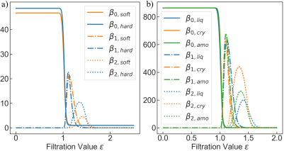
Figure 5: The variation of average Betti numbers with $\epsilon$ for a) all neighborhoods with a radius $r=2.5$ of particle samples at time step $t=100+100\times(k-1),k\in[1,10]\cap\mathbb{N}$, and b) all systems sampled at time step $t=100+25\times(k-1),k\in[1,33]\cap\mathbb{N}$, from each trajectory in Group 1 and 2.

Firstly, for the entire systems, as depicted in Fig. 4b), crystals exhibit the highest SI values, followed by amorphous solids, with liquids having the lowest. The distinct and non-overlapping interquartile ranges (IQRs) of SI for these three phases allow for effective differentiation in most cases. Notably, the highest SI for liquids is below the lowest SI for crystals, ensuring perfect classification between the two. As shown in Fig. 5b), the mean $\beta_{2}$ peak is distinct for each phase: crystals ($\beta_{2,\text{cry}}$) show the highest peak, amorphous phases ($\beta_{2,\text{amo}}$) slightly lower, and liquids ($\beta_{2,\text{liq}}$) the lowest. This is expected because crystals, with their highly symmetric and periodic structures, exhibit long-range order (LRO), resulting in concentrated and distinct topological features, especially in $H_{1}$ (cycles) and $H_{2}$ (cavities). These factors contribute to the highest SI values. In contrast, amorphous solids, while lacking long-range order (LRO), exhibit some short-range order (SRO), resulting in SI and mean $\beta_{2}$ values lower than those of crystals but higher than those of liquids.

Specifically, the mean $\beta_{2}$ primarily reflects the number of two-dimensional cavities in the system. In crystals, the highly ordered particle arrangement forms well-defined, stable cavities, resulting in a concentrated peak in the mean $\beta_{2}$. In amorphous solids, although long-range periodicity is absent, localized short-range order (SRO) creates a more scattered cavity distribution, resulting in a broader $\beta_{2}$ peak. In the case of liquids, with even less structural coherence, the distribution of cavities is highly random, resulting in the lowest and most diffuse $\beta_{2}$ peak. These differences in topological features directly reflect the degree of structural organization in each phase: crystals exhibit the most ordered and interconnected structures, followed by amorphous solids, and then liquids.

Fig. 6 illustrates the concept of SI by showing the clarity of boundaries in the clusters of $H_{1}$ and $H_{2}$ points across different phases. Clearer cluster boundaries correspond to higher SI values, indicating a more ordered structure. Note that the degree of order here is relative. In the liquids (Fig. 6a)), the clusters of $H_{1}$ and $H_{2}$ points are diffuse with indistinct boundaries, resulting in the lowest SI value. The amorphous solids (Fig. 6c)) shows the boundaries of moderate clarity, yielding SI values between those of the liquids and crystals. In contrast, the crystals (Fig. 6b)) has the most clearly defined boundaries, corresponding to the highest SI value.

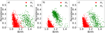
Figure 6: The $H_{1}$ and $H_{2}$ points for the entire systems from selected trajectories as follow: a) for liquid ($\text{Traj}(T^{(2)}_{9})$ at time step $t=900$); b) for crystal ($\text{Traj}(T^{(1)}_{5})$ at time step $t=900$); c) for amorphous ($\text{Traj}(T^{(2)}_{1})$ at time step $t=200$).

Secondly, for particle environments, as illustrated in Fig. 4a), hard particles exhibit higher SI values than soft particles in their neighborhoods. As the neighborhood radius $r$ increases, the IQRs of the neighborhoods of hard and soft particles diverge, and the number of outliers decreases. This suggests that small-scale structures progressively merge as $r$ increases, leading to a more coherent understanding of the global structure. The neighborhoods of hard particles tend to exhibit SI distributions typical of solids, whereas those of soft particles show more liquid-like characteristics, as seen in Fig. 4b). Furthermore, as shown in Fig. 5a), the mean $\beta_{2}$ of hard-particle neighborhoods peaks higher than that of soft-particle neighborhoods. When $\epsilon\in[0,1]$, the mean $\beta_{0}$ for hard-particle neighborhoods is greater, indicating that these neighborhoods contain more particles. This is expected because hard particles generally reside in environments with strong symmetry and SRO, where particles are densely packed. This symmetry and dense packing enhance resistance to rearrangement, giving hard particles solid-like properties. In contrast, soft particles are found in less symmetric or ordered environments, exhibiting more liquid-like behavior.

Physically, these topological differences can be understood by considering the role of cavities (mean $\beta_{2}$) and connected components (mean $\beta_{0}$). The higher mean $\beta_{2}$ peaks in hard-particle neighborhoods reflect well-defined cavities resulting from tight, symmetric packing, indicative of solid-like stability. Besides, higher mean $\beta_{0}$ values in hard-particle neighborhoods also indicate greater local connectivity, reflecting a higher number of neighboring particles. In contrast, soft-particle neighborhoods, with more dispersed and irregular cavity structures, indicate environments where particles are less tightly bound, making these neighborhoods more liquid-like. The lower connectivity in these environments, indicated by mean $\beta_{0}$, further emphasizes their liquid-like mobility.

Fig. 7 shows the $H_{1}$ and $H_{2}$ points in the neighborhoods of soft and hard particles. For soft particles (Fig. 7a)), the $H_{1}$ and $H_{2}$ clusters nearly merge, yielding lower SI values, which indicate low symmetry and disorder. In contrast, hard particles (Fig. 7b)) exhibit relatively clear cluster boundaries, resulting in higher SI values that reflect a more symmetric and ordered environment. In comparison with Fig. 6, the neighborhoods of soft particles resemble liquid characteristics, while those of hard particles are more solid-like.

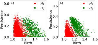
Figure 7: The $H_{1}$ and $H_{2}$ points of neighborhoods with a radius $r=2.5$, after randomly sampling 100 soft particles and 100 hard particles from from each trajectory in Group 1 and 2 at time step $t=100+100\times(k-1),k\in[1,10]\cap\mathbb{N}$ for a) soft particles, and b) hard particles.

In crystalline environments, the local symmetry and SRO around hard particles lead to higher $\beta_{2}$, as stable cavities form in their surroundings. With a small radius $r$, the neighborhood around a hard particle may exhibit properties similar to those in amorphous materials, with evident SRO and local symmetry. However, as the neighborhood radius increases, periodicity, global symmetry, and LRO begin to emerge, transitioning the topological features from local to global. This shift results in increased $\beta_{2}$ and SI values as more extensive, higher-dimensional structures develop, reflecting the mechanism through which LRO and global symmetry are established. In contrast, soft particles, especially those in liquids, due to their higher fluidity and lack of such ordered structures, exhibit lower $\beta_{2}$ and SI values, indicative of the randomness and instability of the topological features in liquid-like environments.

V.2 Phase Transitions

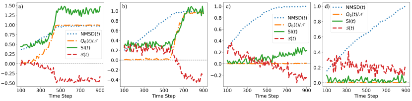
Figure 8: The Normalized MSD (abbreviated as $\text{NMSD}(t)$, normalizing the MSD into $[0,1]$), $Q_{6}(t)/\mathscr{N}$, $\text{SI}(t)$, and $\mathcal{S}(t)$ where $t=100+10\times(i-1)$, $i\in[1,81]\cap\mathbb{N}$ on the selected trajectories a) $\text{Traj}(T_{3}^{(2)})$ containing a whole transition from amorphous to crystal; b) $\text{Traj}(T_{6}^{(2)})$ containing a whole transition from liquid to crystal; c) $\text{Traj}_{\text{KA}}^{(1)}$ containing a process of vitrification from a supercooled liquid; d) $\text{Traj}_{\text{KA}}^{(2)}$ remaining liquid phase during quenching.

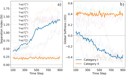
Figure 9: The a) Separation Index $\text{SI}(t)$ and b) Global Softness $\mathcal{S}(t)$, where $t=100+10\times(i-1)$, $i\in[1,81]\cap\mathbb{N}$, for trajectories in Group 2, denoted as $\text{Traj}(T^{(2)}_{k}),k\in[1,10]\cap\mathbb{N}$. These 10 trajectories are divided into two categories: those with $k\leq 6$ (Category I) crystallized, while those with $k\geq 7$ (Category II) remained liquid. The metrics over time for each trajectory are shown as faded dashed lines, with bold lines indicating the average in each category—blue for Category I and orange for Category II.

We tracked the evolution in four metrics including normalized MSD, $Q_{6}(t)/\mathscr{N}$, $\text{SI}(t)$ and $\mathcal{S}(t)$ over time on ten trajectories in test group (Group 2), i.e., $\text{Traj}(T^{(2)}_{k}),k\in[1,10]\cap\mathbb{N}$, as well as two trajectories in Group 3, i.e., $\text{Traj}_{\text{KA}}^{(1)}$ and $\text{Traj}_{\text{KA}}^{(2)}$. The data for all metrics are provided in Fig. 17 of Appendix E for reference.

The trajectories in the test set (Group 2) are divided into two categories: Category I, with $k\leq 6$, undergoes complete crystallization from an amorphous or liquid state, while Category II, with $k\geq 7$, remains in the liquid phase. In Fig. 9, the blue solid line shows the average of SI (Fig. 9a)) and Global Softness (Fig. 9b)) for each trajectory in Category I, while the orange solid line shows the same for Category II. In Category I, SI rises sharply as Global Softness decreases, whereas in Category II, SI stays low and stable, with Global Softness remaining at a high positive level. This distinction clearly differentiates crystallized states from non-crystallized ones. Notably, the Global Softness was calculated using a linear SVM explaining 98% of the explained variance, trained in Task 1. In contrast, other three metrics are non-ML based.

In Fig. 8, without loss of generality, we report the evolution of four metrics over time for four representative trajectories: (i) $\text{Traj}(T_{3}^{(2)})$, which undergoes a complete transition from amorphous to crystalline (Fig. 8a); (ii) $\text{Traj}(T_{6}^{(2)})$, which undergoes a complete crystallization from liquid (Fig. 8b); (iii) $\text{Traj}_{\text{KA}}^{(1)}$, depicting a glass transition from a liquid (Fig. 8c); and (iv) $\text{Traj}_{\text{KA}}^{(2)}$, which remains in the liquid phase during quenching (Fig. 8d).

The order parameter $Q_{6}$ captures the global ordering in the system, particularly six-fold symmetry, and is effective for detecting crystallization, especially from a higher-energy phase (liquid or amorphous) to a more ordered crystalline phase. In liquid or amorphous states, $Q_{6}$ values are typically lower, indicating minimal structural symmetry. However, as the system crystallizes, $Q_{6}$ rises sharply, signaling the emergence of LRO. As local particle order increases and aligns with the global structure, $Q_{6}$ gradually rises. A sharp increase or spike in $Q_{6}$ during this transition (Fig. 8a) and Fig. 8b)) clearly indicates the formation of LRO in crystals.

However, $Q_{6}$ lacks sufficient sensitivity to subtle variations in SRO and thus cannot effectively distinguish between liquid and amorphous solids (see Fig. 8c)). Therefore, $Q_{6}$ needs to be combined with MSD to effectively differentiate these three phases (liquids, amorphous solids, and crystals). Particle mobility in the system is quantified by MSD, which measures the average displacement of particles over a specified time interval. In the liquids, particles move freely, and MSD increases rapidly in a linear manner, indicating high mobility. After crystallization, the MSD stabilizes, indicating that particles are restricted to fixed positions (see Fig. 8b)). Notably, in the amorphous solids that are undergoing crystallization, the MSD also increases, but more gradually than in the liquids. This slower increase reflects the gradual ordering of local structures, as opposed to random diffusion (see Fig. 8a)).

We propose that $\text{SI}(t)$ is highly effective for distinguishing among liquids, amorphous solids, and crystals. In Fig. 8a), $\text{SI}(t)$ increases steadily during the crystallization of the amorphous phase, indicating a transition from a disordered to an ordered structure. Similarly, Fig. 8b) shows a sharp rise in $\text{SI}(t)$ during liquid crystallization, indicating a shift of the system to a solid state. In Fig. 8c), $\text{SI}(t)$ captures the increase in SRO as the system quenches from liquid to amorphous, indicated by the upward turn in the curve. In contrast, $Q_{6}$ fails to capture these subtle changes and remains close to zero. Finally, Fig. 8d) shows that $\text{SI}(t)$ remains stable during quenching in the liquids, with minimal changes in SRO. Notably, $\text{SI}(t)$ demonstrates exceptional sensitivity in capturing transitions between two disordered phases (e.g., liquid and amorphous), as consistent with the results observed in Fig. 4b). This sensitivity significantly surpasses that of traditional order parameters such as $Q_{6}$, which exhibit minimal or no ability to distinguish between disordered phases.

In addition, $\mathcal{S}(t)$ captures the fluidity trend of the system, offering insights into both its current state and potential future behavior. Note that, $\mathcal{S}(t)$ was trained on the training set (Group 1, LJ system) and applied into the test set (Group 2, LJ system) and Group 3 (KA system). When applied to Group 2, a positive $\mathcal{S}(t)$ indicates a trend towards solidification, while a negative value suggests the system is likely to remain fluid. By correlating with potential energy in the system, $\mathcal{S}(t)$ captures both current structural changes and the potential evolution of fluidity over time. As the system transitions from an amorphous phase (see Fig. 8a)) or a liquid phase (see Fig. 8b)) to a crystalline phase, a sharp drop in $\mathcal{S}(t)$ indicates a substantial reduction in fluidity and the stabilization of the crystalline phase. When applied to Group 3 (KA mixture, see Fig. 8c) and Fig. 8d)), $\mathcal{S}(t)$ required a correction to accurately reflect the positive and negative relationships (see Fig. 16 of Appendix D), as the differences in atomic configurations caused systematic shifts in the absolute scale of fluidity. However, it only serves as a reference, and its shift does not impact the presentation of the underlying principles. Therefore, we ignore exploring the correction mechanism as it is not the key factor. If the purpose is solely to track the fluidity on a single trajectory, this correction to align the zero point is not necessary. On the contrary, as mentioned at the beginning of this paragraph, when applied to Group 2 (LJ system), $\mathcal{S}(t)$ required no such adjustment (see Fig. 8b)), indicating that its positive and negative relationships can be directly used without any corrections.

Overall, our proposed SI and Global Softness not only effectively detect phase transitions but also reflect the harmonious integration of ML and non-ML approaches within our PH-based framework.

VI Conclusion and Perspective

We employed persistent homology (PH) to develop a unified mathematical framework for both local and global characterization in disordered systems. This approach produces high-performance descriptors for interpretable machine learning (ML) and offers deep insights into the structure-function relationships in these systems. It reveals crucial links between local particle environments and global structures, predicting particle rearrangement and classifying phases in a universal framework. Our proposed Separation Index (SI) effectively captures the differences in order among liquid, amorphous, and crystalline phases in multi-particle systems, providing an explanation for the mechanism of long-range order formation. Besides, SI, in conjunction with Global Softness, achieves precise detection of phase transitions through non-ML and ML pathways, respectively. Furthermore, complexity science suggests that global behavior in a system arises from nonlinear interactions among local components, rather than from simple linear addition. Our unified framework fundamentally avoids the issue of nonlinear adding, while treating local and global characteristics as homogeneous representations. This offers a novel perspective for research in complexity science.

We acknowledge that there are certain limitations to our approach as it currently stands. Firstly, computational complexity limits its scalability and cost-effectiveness when applied to large datasets. Secondly, while the method effectively captures topological features, its applicability may be limited in QSAR tasks that depend on geometric properties like metrics and curvature. Thirdly, although the framework performs well in specific multi-particle systems constrained by Lennard-Jones potentials, its generalizability to other disordered systems and diverse dynamical processes remains unverified. Finally, regarding the Separation Index (SI) and its relationship to order and symmetry, current validation is computational, lacking rigorous proof of how SI quantitatively reflects these physical characteristics.

Our future work will naturally focus on addressing these limitations. Firstly, improving computational efficiency to handle systems with over $10^{5}$ particles will be a key objective in scaling our approach. Secondly, we will consider combining our PH-based approach with computational conformal geometry [85, 86, 87] to better accommodate targets requiring precise geometric detail, such as defects and polycrystals, and tasks like atomic-scale defect reconstruction or complex surface structuring. Thirdly, we plan to explore dynamical processes beyond phase transitions, including defect migration and reconstruction, particle diffusion and aggregation, and phase separation with multicomponent interactions. Lastly, we aim to rigorously establish how SI captures order and symmetry in the system, and develop its mathematical foundation in relation to underlying physics.

The code related to this article is available at https://github.com/anwanguow/PH_structural.

Appendix A The Protocols of MD Simulations

For LJ systems, the parameters of the Lennard-Jones potentials are: $\epsilon=1$, $\sigma=1$, cutoff radius $r_{c}=3.5\sigma$ and mass $m=1M$. We have adopted a tail correction as the truncation scheme. The computational protocol we have followed begins with a linearly quench of the liquid from $T_{\text{init}}=1.25$ to a given temperature $T_{\text{final}}$ in 20 steps. Then, we perform a $1000$ steps equilibration at temperature $T_{\text{final}}$. These simulations have been conducted within the NPT ensemble with an isotropic pressure $P=5.68(\epsilon/{\sigma^{3}})$, enforced via a chain of five thermostats coupled to a Nosé–Hoover barostat [88] (which accounts for the Martyna-Tobias-Klein correction [89]). The damping parameter of the barostat is $0.5t^{*}$, where $t^{*}=0.002(m*\sigma^{2}/\epsilon)^{1/2}$. For convenience, we denote the trajectory corresponding to its temperature $T$ as $\text{Traj}(T)$. All these trajectories were generated using the same initial positions and velocities for each particle. These settings are the same as those adopted in Ref. [90].

For KA mixtures [73, 74], we use the parameter setting: $\epsilon_{AA}=\sigma_{AA}=1$, $\epsilon_{AB}=1.5$, $\sigma_{AB}=0.8$, $\epsilon_{BB}=0.5$, $\sigma_{BB}=0.88$. We started from $T_{\text{init}}=1.25$ and quenched the system to the final temperature $T_{\text{final}}$, which is low enough to guarantee the solidification of the system, either in the crystalline or amorphous phase. The details of these MD simulations are identical to those utilised for the homogeneous LJ system including the system size - 864 particles in total, with the proportion of B particles as $\chi_{B}=0.2$. We generated two trajectories within the time step of $1000$, where one time step equals to $100\times(0.2*(m*\sigma^{2}/\epsilon)^{1/2})$ in LJ reduced units. We denote these two trajectories as $\text{Traj}_{\text{KA}}^{(1)}$ and $\text{Traj}_{\text{KA}}^{(2)}$ (Group 3). The $T_{\text{final}}$ settings are: (1) for $\text{Traj}_{\text{KA}}^{(1)}$, $T_{\text{final}}=0.5$.; (2) for $\text{Traj}_{\text{KA}}^{(2)}$, $T_{\text{final}}=1.0$.

Appendix B Implementation of SVM

This article uses two kinds of SVMs as $f$:

SVM with Linear Kernel

• Decision function:

  $$f(\mathbb{X})=\mathbb{X}\cdot\mathbb{w}+u$$

  where $\mathbb{w}$ is the weight vector, $u$ is the bias term.

• Objective function:

  $$\mathop{\min}_{\mathbb{w},b}\frac{1}{2}||\mathbb{w}||_{2}^{2}+C\sum_{i=1}^{N}\mathop{\max}(0,1-y_{i}(\mathbb{X}_{(i)}\cdot\mathbb{w}+u))$$

  where $C$ is the regularization parameter that controls the trade-off between the regularization term and the loss term.

• Hyperparameters: $C\in[0.001,1000]$, log-scaled.

SVM with RBF Kernel

• RBF kernel:

  $$K(\mathbb{X}_{(i)},\mathbb{X}_{(j)})=\mathop{\exp}(-\gamma||\mathbb{X}_{(i)}-\mathbb{X}_{(j)}||^{2})$$

  where $\gamma$ is a parameter that controls the extent of the influence of each data point on the similarity measure.

• Decision function:

  $$f(\mathbb{X})=\sum_{i=1}^{N}\alpha_{i}y_{i}K(\mathbb{X},\mathbb{X}_{(i)})+u$$

  where $\alpha_{i}$ are Lagrange multipliers quantifying the importance of $X_{(i)}$ within the decision function and $u$ is the bias term.

• Objective function:

  $$\mathop{\max}_{\alpha}\left[\sum_{i=1}^{N}\alpha_{i}-\frac{1}{2}\sum_{i=1}^{N}\sum_{j=1}^{N}\alpha_{i}\alpha_{j}y_{i}y_{j}K(\mathbb{X}_{(i)},\mathbb{X}_{(j)})\right]$$

  subject to the constraints:

  $$\sum_{i=1}^{N}\alpha_{i}y_{i}=0\text{ and }0\leq\alpha_{i}\leq C,\forall i.$$

  Here, $C$ is a regularization parameter, and $\alpha_{i}$ are Lagrange multipliers relative to each sample.

• Hyperparameters: (1) $C\in[0.001,1000]$, log-scaled; (2) $\gamma\in[0.001,1000]$, log-scaled.

For consistency, we set the hyperparameter optimization as follows: 10-fold cross-validation for validation, Matthews Correlation Coefficient (MCC)) [91] and accuracy as evaluation metrics, and a Bayesian optimizer [92] with 200 steps using Expected Improvement per second plus (EIps) as the acquisition function. For the multi-class strategy (only for Task 2), we try the methods of One-vs-One and One-vs-All at the same time, and select the best-performing one.

Appendix C Parameter Selection

C.1 The parameter selection for the PI

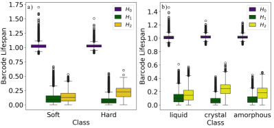
Figure 10: Box plots of the barcode lifespan (persistence) of a) all neighborhoods with a radius $r=2.5$ of particle samples at time step $t=100+100\times(k-1),k\in[1,10]\cap\mathbb{N}$, and b) all systems sampled at time step $t=100+25\times(k-1),k\in[1,33]\cap\mathbb{N}$, from each trajectory in Group 1 and 2.

Here, the parameters we need to set are minBD, maxBD, $\tau$, $\mathfrak{M}$, $\mathfrak{N}$, and $\sigma$.

The parameters minBD and maxBD are used to filter out features with very short or excessively long persistence. Based on the analysis in Fig. 10, all $H_{1}$ and $H_{2}$ features have lifetimes below 0.75, and most $H_{0}$ features are below 1.5. Therefore, setting maxBD to 1.5 is sufficient to capture all relevant features. To avoid numerical errors, minBD is set to -0.1.

In the formula $\mathbb{I}^{(P)}_{p}=\sum_{q=1}^{\mathcal{N}}\mathbb{V}^{(P)}_{p,q}\cdot e^{-\tau(r_{q}-r_{1})}$, the decay factor $\tau$ is chosen to balance the rate of decay, ensuring $\mathbb{V}_{p,q}^{(P)}$ decays from 100% to 10% as $r_{q}$ increases from 1 to 5. Based on the decay curves in Fig. 11, we set $\tau=0.57$ as the most appropriate value.

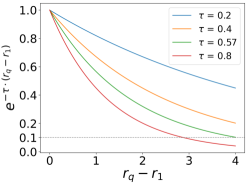
Figure 11: The four curves in different color respectively represent the change in $e^{-\tau(r_{q}-r_{1})}$ as $r_{q}-r_{1}$ increases from 0 to 4 (or, $r_{q}$ increases from 1 to 5) under the premise of taking different values of $\tau$. The gray horizontal dashed line is $y=0.1$.

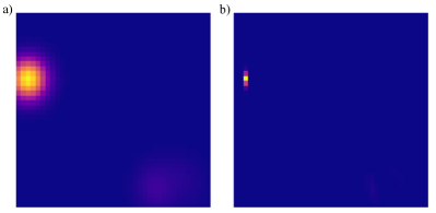
Figure 12: The examples for a) an unclear PI, with $\tau$ = 0.1, and b) a clear PI, with $\tau=0.002$, which are both generated from the frame corresponding to $\text{Traj}(T_{4}^{(2)})$ at time step $t=100$.

To balance computational efficiency and model performance, we set $\mathfrak{M}=\mathfrak{N}=40$ initially and treat $\sigma$ as a hyperparameter. The selection of $\sigma$ follows a two-stage process: (1) coarse screening; (2) fine-tuning.

Coarse Screening: In this stage, we visually inspected the clarity of the PI generated with different values of $\sigma$. A smaller $\sigma$ preserves more details of topological features, while a larger $\sigma$ smooths the image, reducing the impact of individual points, as shown in Fig. 12. By observing the degree of blurring in the PI, we quickly identified a suitable range of $\sigma$ between 0.001 and 0.01.

Table 3: Performance comparison of different values of $\tau\in[0.001,0.01]$ in Task 2.

SVM (98% Var)	Linear		RBF Kernel
$\sigma$	ACC	MCC	ACC	MCC
0.001	95.5%	0.760	94.8%	0.750
0.002	94.5%	0.730	95.5%	0.760
0.003	95.5%	0.764	95.5%	0.764
0.004	95.5%	0.764	95.5%	0.764
0.005	95.8%	0.757	95.2%	0.757
0.006	95.2%	0.743	95.5%	0.760
0.007	96.1%	0.763	95.2%	0.753
0.008	95.5%	0.764	95.2%	0.753
0.009	95.8%	0.767	95.5%	0.760
0.010	96.1%	0.763	95.5%	0.760

Fine-Tuning: In this stage, we treated $\sigma$ as a hyperparameter and refined it through iterative training and validation. Using both two kinds of SVMs, we found that while $\sigma$ had minimal impact on overall performance, as listed in Table 3. The model achieved the optimal performance with $\sigma=0.01$.

C.2 The Parameter Selection for Rearrangement Tendency (Task 1)

Here, the parameters we need to set are $t_{R/2}$ and $p_{c}$, aligned with Ref. [90]. Fig. 13, 14, and 15 are all adapted from Ref. [90]. The settings is based on the statistics on Group 1 (Set 1), and we cannot use the data in the Group 2 (Set 2) at this stage to avoid the data leakage.

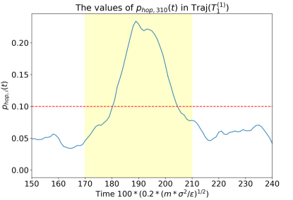
Figure 13: The evolution of $p_{\text{hop}}$ for a selected particle (No.310) over a period of time under the lowest temperature (i.e., $T^{(1)}_{1}$). The yellow region represents the interval with the time length of $2t_{R/2}$, encompassing a complete rearrangement, which means $p_{hop}$ rises above $p_{c}$ and then falls back below $p_{c}$. The red-dotted line is the selected $p_{c}=0.1$.

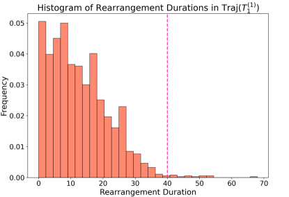
Figure 14: The histogram of rearrangement duration in $\text{Traj}(T^{(1)}_{1})$, corresponding to the lowest temperature and the system with the lowest mobility. The red-dotted line is the selected $t_{R}=40$, which equals to $2t_{R/2}$.

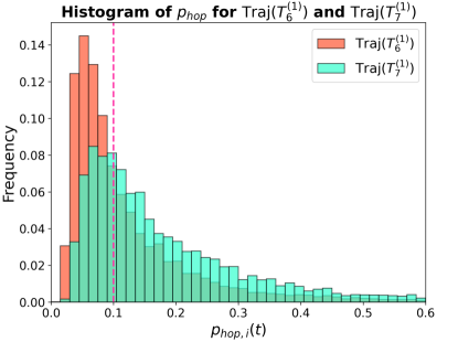
Figure 15: The histogram of the value of $p_{\text{hop}}$ in $\text{Traj}(T^{(1)}_{6})$ and $\text{Traj}(T^{(1)}_{7})$. The onset temperature $T^{(1)}_{c}$ of crystallization separates $T^{(1)}_{6}$ and $T^{(1)}_{7}$, i.e., $T^{(1)}_{6}<T^{(1)}_{c}<T^{(1)}_{7}$. The red-dotted line is the selected $p_{c}=0.1$. The reason for setting $p_{c}=0.1$ is when $p_{\text{hop}}<p_{c}$, the frequency of $p_{\text{hop}}$ in $\text{Traj}(T^{(1)}_{6})$ is larger than that in $\text{Traj}(T^{(1)}_{7})$; when $p_{\text{hop}}\geq p_{c}$, the frequency of $p_{\text{hop}}$ in $\text{Traj}(T^{(1)}_{6})$ is smaller than that in $\text{Traj}(T^{(1)}_{7})$. $p_{c}=0.1$ is the value at which the relative size of two frequency of $\text{Traj}(T^{(1)}_{6})$ and $\text{Traj}(T^{(1)}_{7})$ reverse.

To select $t_{R/2}$, we use the lowest temperature $T^{(1)}_{1}$ as a reference because it corresponds to the system’s lowest mobility. The interval $[t-t_{R/2},t+t_{R/2}]$ should encompass as many complete rearrangements as possible at this low mobility, as shown in Fig. 13. The yellow region marks a full rearrangement, where $p_{\text{hop}}$ rises above and then falls below $p_{c}$. As seen in Fig. 14, most rearrangements at this reference temperature occur within $t_{R}=40$, so we set $t_{R/2}=20$.

As shown in Fig. 15, we chose $p_{c}=0.1$ because it effectively separates the majority of particles in two trajectories above and below the crystallization onset temperature, i.e., $T^{(1)}_{6}$ and $T^{(1)}_{7}$. The $p_{\text{hop},i}(t)$ values are mostly significantly greater or less than $p_{c}=0.1$, respectively. Specifically, $T^{(1)}_{6}$ is the highest temperature at which crystallization occurs, while $T^{(1)}_{7}$ is the lowest temperature where the liquid phase is maintained, both of which are critical for this analysis. By plotting the histograms of $p_{\text{hop}}$ in $\text{Traj}(T^{(1)}_{6})$ and $\text{Traj}(T^{(1)}_{7})$, we determined that $p_{c}=0.1$ is the value at which the relative sizes of the two distributions reverse.

Appendix D Correctness of Global Softness

Fig. 16 demonstrate the correction by a downward shift of 0.15 when applying the model to the KA systems. After correction, the positive or negative sign of Global Softness can indicate the class of fluidity trend.

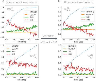
Figure 16: The global softness $\mathcal{S}(t)$ (red lines) shown in a) is before the correction, while the softness shown in b) is after the correction by a downward shift of $0.15$.

Appendix E Extra Data

The datasets for Task 2 are listed in Table 4, and the evolution of all four metrics over time for each trajectory in Group 2 (testing group) are listed in Fig. 17.

Table 4: The labels, i.e., $y_{\text{entire},t}^{(T^{(1)}_{i})}$ for Set 3 (sampled from Group 1) and $y_{\text{entire},t}^{(T^{(2)}_{i})}$ for Set 4 (sampled from Group 2). In this table, 0 represents liquid, 1 represents crystal, and 2 represents amorphous. The $i$-th row represents trajectory $\text{Traj}(T_{i}^{(1\text{ or }2)})$, and the $j$-th column represents the sample point at $t=100+25\times(j-1)$.

Set 3 (sampled from Group 1)
2	2	2	2	2	2	2	2	2	2	2	2	2	2	2	2	2	2	2	2	2	2	2	2	2	2	2	2	2	2	2	2	2
2	2	2	2	2	2	2	2	2	2	1	1	1	1	1	1	1	1	1	1	1	1	1	1	1	1	1	1	1	1	1	1	1
2	2	2	2	2	2	1	1	1	1	1	1	1	1	1	1	1	1	1	1	1	1	1	1	1	1	1	1	1	1	1	1	1
2	2	2	2	1	1	1	1	1	1	1	1	1	1	1	1	1	1	1	1	1	1	1	1	1	1	1	1	1	1	1	1	1
0	0	0	0	0	0	0	0	0	0	0	0	0	0	0	0	0	0	0	0	0	0	1	1	1	1	1	1	1	1	1	1	1
0	0	0	0	0	0	0	0	0	0	0	0	0	0	0	0	0	0	0	0	0	0	0	0	0	0	0	0	0	0	0	0	0
0	0	0	0	0	0	0	0	0	0	0	0	0	0	0	0	0	0	0	0	0	0	0	0	0	0	0	0	0	0	0	0	0
0	0	0	0	0	0	0	0	0	0	0	0	0	0	0	0	0	0	0	0	0	0	0	0	0	0	0	0	0	0	0	0	0
0	0	0	0	0	0	0	0	0	0	0	0	0	0	0	0	0	0	0	0	0	0	0	0	0	0	0	0	0	0	0	0	0
0	0	0	0	0	0	0	0	0	0	0	0	0	0	0	0	0	0	0	0	0	0	0	0	0	0	0	0	0	0	0	0	0
Set 4 (sampled from Group 2)
2	2	2	2	2	2	2	2	2	2	2	2	2	2	2	2	2	2	2	2	2	2	2	1	1	1	1	1	1	1	1	1	1
2	2	2	2	2	2	2	2	2	2	2	2	2	1	1	1	1	1	1	1	1	1	1	1	1	1	1	1	1	1	1	1	1
2	2	2	2	2	2	2	2	2	2	2	2	1	1	1	1	1	1	1	1	1	1	1	1	1	1	1	1	1	1	1	1	1
2	2	2	1	1	1	1	1	1	1	1	1	1	1	1	1	1	1	1	1	1	1	1	1	1	1	1	1	1	1	1	1	1
0	0	0	0	0	0	0	0	0	0	0	1	1	1	1	1	1	1	1	1	1	1	1	1	1	1	1	1	1	1	1	1	1
0	0	0	0	0	0	0	0	0	0	0	0	0	0	0	0	0	0	0	0	0	1	1	1	1	1	1	1	1	1	1	1	1
0	0	0	0	0	0	0	0	0	0	0	0	0	0	0	0	0	0	0	0	0	0	0	0	0	0	0	0	0	0	0	0	0
0	0	0	0	0	0	0	0	0	0	0	0	0	0	0	0	0	0	0	0	0	0	0	0	0	0	0	0	0	0	0	0	0
0	0	0	0	0	0	0	0	0	0	0	0	0	0	0	0	0	0	0	0	0	0	0	0	0	0	0	0	0	0	0	0	0
0	0	0	0	0	0	0	0	0	0	0	0	0	0	0	0	0	0	0	0	0	0	0	0	0	0	0	0	0	0	0	0	0

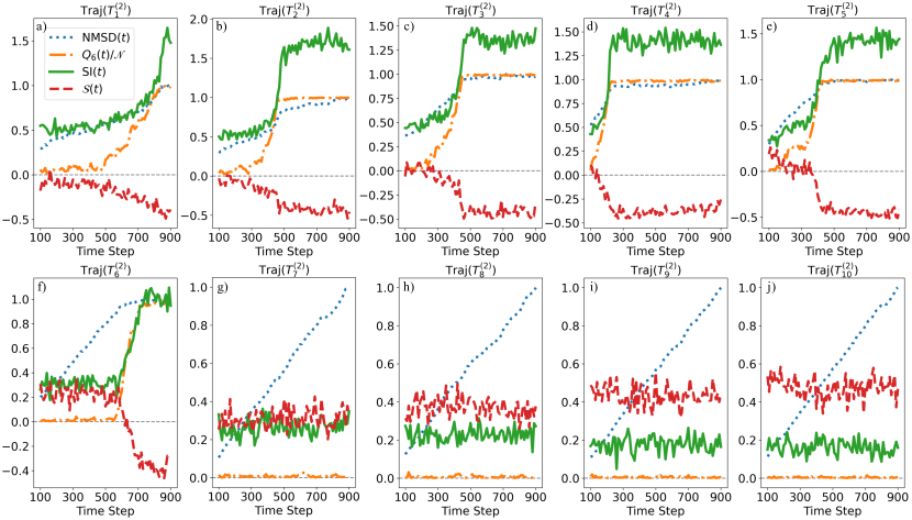
Figure 17: The Normalized MSD (abbreviated as $\text{NMSD}(t)$, normalizing the MSD into $[0,1]$), $Q_{6}(t)/\mathscr{N}$, $\text{SI}(t)$, and $\mathcal{S}(t)$ where $t=100+10\times(i-1)$, $i\in[1,81]\cap\mathbb{N}$ on all trajectories on Group 2 (Testing Group), containing a) $\text{Traj}(T_{1}^{(2)})$, b) $\text{Traj}(T_{2}^{(2)})$, c) $\text{Traj}(T_{3}^{(2)})$, d) $\text{Traj}(T_{4}^{(2)})$, e) $\text{Traj}(T_{5}^{(2)})$, f) $\text{Traj}(T_{6}^{(2)})$, g) $\text{Traj}(T_{7}^{(2)})$, h) $\text{Traj}(T_{8}^{(2)})$, i) $\text{Traj}(T_{9}^{(2)})$, and j) $\text{Traj}(T_{10}^{(2)})$.

References

- Zhang et al. [2019] J. Zhang, Y. Zhao, C. Chen, Y.-C. Huang, C.-L. Dong, C.-J. Chen, R.-S. Liu, C. Wang, K. Yan, Y. Li, et al., Tuning the coordination environment in single-atom catalysts to achieve highly efficient oxygen reduction reactions, Journal of the American Chemical Society 141, 20118 (2019).
- Li et al. [2020] X. Li, H. Rong, J. Zhang, D. Wang, and Y. Li, Modulating the local coordination environment of single-atom catalysts for enhanced catalytic performance, Nano Research 13, 1842 (2020).
- Cowley [1965] J. Cowley, Short-range order and long-range order parameters, Physical Review 138, A1384 (1965).
- Capella and Krzywicki [1978] A. Capella and A. Krzywicki, Unitarity corrections to short-range order: Long-range rapidity correlations, Physical Review D 18, 4120 (1978).
- Ferrari et al. [2023] A. Ferrari, F. Körmann, M. Asta, and J. Neugebauer, Simulating short-range order in compositionally complex materials, Nature Computational Science 3, 221 (2023).
- Fuller [1959] W. Fuller, Hydrogen bond lengths and angles observed in crystals, The Journal of Physical Chemistry 63, 1705 (1959).
- Geisinger et al. [1985] K. Geisinger, G. Gibbs, and A. Navrotsky, A molecular orbital study of bond length and angle variations in framework structures, Physics and Chemistry of Minerals 11, 266 (1985).
- Laskowski et al. [1993] R. A. Laskowski, D. S. Moss, and J. M. Thornton, Main-chain bond lengths and bond angles in protein structures, Journal of molecular biology 231, 1049 (1993).
- Shirley et al. [1995] W. A. Shirley, R. Hoffmann, and V. S. Mastryukov, An approach to understanding bond length/bond angle relationships, The Journal of Physical Chemistry 99, 4025 (1995).
- Hohenberg [1967] P. C. Hohenberg, Existence of long-range order in one and two dimensions, Physical Review 158, 383 (1967).
- White and Geballe [2013] R. M. White and T. H. Geballe, Long Range Order in Solids: Solid State Physics (Elsevier, 2013).
- Yang [1962] C. N. Yang, Concept of off-diagonal long-range order and the quantum phases of liquid he and of superconductors, Reviews of Modern Physics 34, 694 (1962).
- Pershan [1988] P. S. Pershan, Structure of liquid crystal phases, Vol. 23 (World Scientific, 1988).
- Izyumov and Syromyatnikov [2012] Y. A. Izyumov and V. N. Syromyatnikov, Phase transitions and crystal symmetry, Vol. 38 (Springer Science & Business Media, 2012).
- Hirschfelder et al. [1937] J. Hirschfelder, D. Stevenson, and H. Eyring, A theory of liquid structure, The Journal of Chemical Physics 5, 896 (1937).
- Takayama [1976] S. Takayama, Amorphous structures and their formation and stability, Journal of Materials Science 11, 164 (1976).
- Jette and Foote [1935] E. R. Jette and F. Foote, Precision determination of lattice constants, The Journal of Chemical Physics 3, 605 (1935).
- Alexander [1998] S. Alexander, Amorphous solids: their structure, lattice dynamics and elasticity, Physics reports 296, 65 (1998).
- Drabold [2009] D. Drabold, Topics in the theory of amorphous materials, The European Physical Journal B 68, 1 (2009).
- Glazer et al. [2012] M. Glazer, G. Burns, and A. N. Glazer, Space groups for solid state scientists (Elsevier, 2012).
- Aroyo and Wondratschek [2013] M. I. Aroyo and H. Wondratschek, International tables for crystallography (Wiley Online Library, 2013).
- De Wolff [1974] P. De Wolff, The pseudo-symmetry of modulated crystal structures, Acta Crystallographica Section A: Crystal Physics, Diffraction, Theoretical and General Crystallography 30, 777 (1974).
- Dressel et al. [2014] C. Dressel, T. Reppe, M. Prehm, M. Brautzsch, and C. Tschierske, Chiral self-sorting and amplification in isotropic liquids of achiral molecules, Nature chemistry 6, 971 (2014).
- Agarwala et al. [2020] A. Agarwala, V. Juričić, and B. Roy, Higher-order topological insulators in amorphous solids, Physical Review Research 2, 012067 (2020).
- Bernal [1964] J. D. Bernal, The bakerian lecture, 1962. the structure of liquids, Proceedings of the Royal Society of London. Series A, Mathematical and Physical Sciences 280, 299 (1964).
- Behler and Parrinello [2007] J. Behler and M. Parrinello, Generalized neural-network representation of high-dimensional potential-energy surfaces, Physical review letters 98, 146401 (2007).
- Behler [2011] J. Behler, Atom-centered symmetry functions for constructing high-dimensional neural network potentials, The Journal of chemical physics 134 (2011).
- Bartók et al. [2013] A. P. Bartók, R. Kondor, and G. Csányi, On representing chemical environments, Physical Review B—Condensed Matter and Materials Physics 87, 184115 (2013).
- Landau [1936] L. Landau, The theory of phase transitions, Nature 138, 840 (1936).
- Landau et al. [1937] L. D. Landau et al., On the theory of phase transitions, Zh. eksp. teor. Fiz 7, 926 (1937).
- Steinhardt et al. [1983] P. J. Steinhardt, D. R. Nelson, and M. Ronchetti, Bond-orientational order in liquids and glasses, Physical Review B 28, 784 (1983).
- Ten Wolde et al. [1995] P. R. Ten Wolde, M. J. Ruiz-Montero, and D. Frenkel, Numerical evidence for bcc ordering at the surface of a critical fcc nucleus, Physical review letters 75, 2714 (1995).
- Patterson [1934] A. L. Patterson, A fourier series method for the determination of the components of interatomic distances in crystals, Physical Review 46, 372 (1934).
- Sheng et al. [2006] H. Sheng, W. Luo, F. Alamgir, J. Bai, and E. Ma, Atomic packing and short-to-medium-range order in metallic glasses, Nature 439, 419 (2006).
- Bates and Fredrickson [1999] F. S. Bates and G. H. Fredrickson, Block copolymers—designer soft materials, Physics today 52, 32 (1999).
- Thorpe [1983] M. F. Thorpe, Continuous deformations in random networks, Journal of Non-Crystalline Solids 57, 355 (1983).
- Frank [1952] F. C. Frank, Supercooling of liquids, Proceedings of the Royal Society of London. Series A. Mathematical and Physical Sciences 215, 43 (1952).
- Finney [1970] J. Finney, Random packings and the structure of simple liquids. i. the geometry of random close packing, Proceedings of the Royal Society of London. A. Mathematical and Physical Sciences 319, 479 (1970).
- Bak et al. [1987] P. Bak, C. Tang, and K. Wiesenfeld, Self-organized criticality: An explanation of the 1/f noise, Physical review letters 59, 381 (1987).
- Olami et al. [1992] Z. Olami, H. J. S. Feder, and K. Christensen, Self-organized criticality in a continuous, nonconservative cellular automaton modeling earthquakes, Physical review letters 68, 1244 (1992).
- Christensen and Moloney [2005] K. Christensen and N. R. Moloney, Complexity and criticality, Vol. 1 (World Scientific Publishing Company, 2005).
- Anderson [1972] P. W. Anderson, More is different: Broken symmetry and the nature of the hierarchical structure of science., Science 177, 393 (1972).
- Carleo et al. [2019] G. Carleo, I. Cirac, K. Cranmer, L. Daudet, M. Schuld, N. Tishby, L. Vogt-Maranto, and L. Zdeborová, Machine learning and the physical sciences, Reviews of Modern Physics 91, 045002 (2019).
- Mehta et al. [2019] P. Mehta, M. Bukov, C.-H. Wang, A. G. Day, C. Richardson, C. K. Fisher, and D. J. Schwab, A high-bias, low-variance introduction to machine learning for physicists, Physics reports 810, 1 (2019).
- Radovic et al. [2018] A. Radovic, M. Williams, D. Rousseau, M. Kagan, D. Bonacorsi, A. Himmel, A. Aurisano, K. Terao, and T. Wongjirad, Machine learning at the energy and intensity frontiers of particle physics, Nature 560, 41 (2018).
- Carleo and Troyer [2017] G. Carleo and M. Troyer, Solving the quantum many-body problem with artificial neural networks, Science 355, 602 (2017).
- Scarselli et al. [2008] F. Scarselli, M. Gori, A. C. Tsoi, M. Hagenbuchner, and G. Monfardini, The graph neural network model, IEEE transactions on neural networks 20, 61 (2008).
- Raissi et al. [2019] M. Raissi, P. Perdikaris, and G. E. Karniadakis, Physics-informed neural networks: A deep learning framework for solving forward and inverse problems involving nonlinear partial differential equations, Journal of Computational physics 378, 686 (2019).
- Bapst et al. [2020] V. Bapst, T. Keck, A. Grabska-Barwińska, C. Donner, E. D. Cubuk, S. S. Schoenholz, A. Obika, A. W. Nelson, T. Back, D. Hassabis, et al., Unveiling the predictive power of static structure in glassy systems, Nature physics 16, 448 (2020).
- Munkres [2018] J. R. Munkres, Elements of algebraic topology (CRC press, 2018).
- Edelsbrunner et al. [2002] Edelsbrunner, Letscher, and Zomorodian, Topological persistence and simplification, Discrete & computational geometry 28, 511 (2002).
- Zomorodian and Carlsson [2004] A. Zomorodian and G. Carlsson, Computing persistent homology, in Proceedings of the twentieth annual symposium on Computational geometry (2004) pp. 347–356.
- Ghrist [2008] R. Ghrist, Barcodes: the persistent topology of data, Bulletin of the American Mathematical Society 45, 61 (2008).
- Poincaré [1899] H. Poincaré, Complémenta l’analysis situs, Rendiconti del Circolo matematico di Palermo 13, 10 (1899).
- Veblen [1912] O. Veblen, An application of modular equations in analysis situs, Annals of Mathematics 14, 86 (1912).
- Hausdorff [1914] F. Hausdorff, Grundzüge der mengenlehre, Vol. 7 (von Veit, 1914).
- Kuratowski [1920] K. Kuratowski, Sur la notion d’ensemble fini, Fundamenta Mathematicae 1, 129 (1920).
- Alexandroff [1929] P. S. Alexandroff, Mémoire sur les espaces topologiques compacts, Verh. Kon. Akad. van Weten. Te Amsterdam 14, 1 (1929).
- Adams et al. [2017] H. Adams, T. Emerson, M. Kirby, R. Neville, C. Peterson, P. Shipman, S. Chepushtanova, E. Hanson, F. Motta, and L. Ziegelmeier, Persistence images: A stable vector representation of persistent homology, Journal of Machine Learning Research 18, 1 (2017).
- Betti [1870] E. Betti, Sopra gli spazi di un numero qualunque di dimensioni, Annali di Matematica Pura ed Applicata (1867-1897) 4, 140 (1870).
- Poincaré [1895] H. Poincaré, Analysis situs (Gauthier-Villars Paris, France, 1895).
- Parzen [1962] E. Parzen, On estimation of a probability density function and mode, The annals of mathematical statistics 33, 1065 (1962).
- Davis et al. [2011] R. A. Davis, K.-S. Lii, and D. N. Politis, Remarks on some nonparametric estimates of a density function, Selected Works of Murray Rosenblatt , 95 (2011).
- Gauss [1877] C. F. Gauss, Theoria motus corporum coelestium in sectionibus conicis solem ambientium, Vol. 7 (FA Perthes, 1877).
- Bauer [2021] U. Bauer, Ripser: efficient computation of vietoris–rips persistence barcodes, Journal of Applied and Computational Topology 5, 391 (2021).
- Einstein [1905] A. Einstein, Über die von der molekularkinetischen theorie der wärme geforderte bewegung von in ruhenden flüssigkeiten suspendierten teilchen, Annalen der physik 4 (1905).
- Jungblut and Dellago [2016] S. Jungblut and C. Dellago, Pathways to self-organization: Crystallization via nucleation and growth, The European Physical Journal E 39, 1 (2016).
- Heaviside [2003] O. Heaviside, Electromagnetic theory, Vol. 237 (American Mathematical Soc., 2003).
- Alder and Wainwright [1957] B. J. Alder and T. E. Wainwright, Phase transition for a hard sphere system, The Journal of chemical physics 27, 1208 (1957).
- Rahman [1964] A. Rahman, Correlations in the motion of atoms in liquid argon, Physical review 136, A405 (1964).
- Hirschfelder et al. [1964] J. O. Hirschfelder, C. F. Curtiss, and R. B. Bird, The molecular theory of gases and liquids (John Wiley & Sons, 1964).
- Jones [1924] J. E. Jones, On the determination of molecular fields.—ii. from the equation of state of a gas, Proceedings of the Royal Society of London. Series A, Containing Papers of a Mathematical and Physical Character 106, 463 (1924).
- Kob and Andersen [1995] W. Kob and H. C. Andersen, Testing mode-coupling theory for a supercooled binary lennard-jones mixture i: The van hove correlation function, Physical Review E 51, 4626 (1995).
- Pedersen et al. [2018] U. R. Pedersen, T. B. Schrøder, and J. C. Dyre, Phase diagram of kob-andersen-type binary lennard-jones mixtures, Physical review letters 120, 165501 (2018).
- Candelier et al. [2010] R. Candelier, A. Widmer-Cooper, J. K. Kummerfeld, O. Dauchot, G. Biroli, P. Harrowell, and D. R. Reichman, Spatiotemporal hierarchy of relaxation events, dynamical heterogeneities, and structural reorganization in a supercooled liquid, Physical review letters 105, 135702 (2010).
- Smessaert and Rottler [2013] A. Smessaert and J. Rottler, Distribution of local relaxation events in an aging three-dimensional glass: Spatiotemporal correlation and dynamical heterogeneity, Physical Review E 88, 022314 (2013).
- Schoenholz et al. [2016] S. S. Schoenholz, E. D. Cubuk, D. M. Sussman, E. Kaxiras, and A. J. Liu, A structural approach to relaxation in glassy liquids, Nature Physics 12, 469 (2016).
- Einstein [1956] A. Einstein, Investigations on the Theory of the Brownian Movement (Courier Corporation, 1956).
- Pearson [1901] K. Pearson, Liii. on lines and planes of closest fit to systems of points in space, The London, Edinburgh, and Dublin philosophical magazine and journal of science 2, 559 (1901).
- Cortes and Vapnik [1995] C. Cortes and V. Vapnik, Support-vector networks, Machine learning 20, 273 (1995).
- Boser et al. [1992] B. E. Boser, I. M. Guyon, and V. N. Vapnik, A training algorithm for optimal margin classifiers, in Proceedings of the fifth annual workshop on Computational learning theory (1992) pp. 144–152.
- Shapley et al. [1953] L. S. Shapley et al., A value for n-person games, Contributions to the Theory of Games 2, 307 (1953).
- Winter [2002] E. Winter, The shapley value, Handbook of game theory with economic applications 3, 2025 (2002).
- Cubuk et al. [2015] E. D. Cubuk, S. S. Schoenholz, J. M. Rieser, B. D. Malone, J. Rottler, D. J. Durian, E. Kaxiras, and A. J. Liu, Identifying structural flow defects in disordered solids using machine-learning methods, Physical review letters 114, 108001 (2015).
- Gu and Yau [2002] X. Gu and S.-T. Yau, Computing conformal structure of surfaces, arXiv preprint cs/0212043 (2002).
- Gu and Yau [2003] X. Gu and S.-T. Yau, Global conformal surface parameterization, in Proceedings of the 2003 Eurographics/ACM SIGGRAPH symposium on Geometry processing (2003) pp. 127–137.
- Gu et al. [2010] D. X. Gu, F. Luo, and S.-T. Yau, Fundamentals of computational conformal geometry, Mathematics in Computer Science 4, 389 (2010).
- Hoover and Holian [1996] W. G. Hoover and B. L. Holian, Kinetic moments method for the canonical ensemble distribution, Physics Letters A 211, 253 (1996).
- Martyna et al. [1994] G. J. Martyna, D. J. Tobias, and M. L. Klein, Constant pressure molecular dynamics algorithms, The Journal of chemical physics 101, 4177 (1994).
- Wang and Sosso [2024] A. Wang and G. C. Sosso, Graph-based descriptors for condensed matter, arXiv preprint arXiv:2408.06156 (2024).
- Matthews [1975] B. W. Matthews, Comparison of the predicted and observed secondary structure of t4 phage lysozyme, Biochimica et Biophysica Acta (BBA)-Protein Structure 405, 442 (1975).
- Snoek et al. [2012] J. Snoek, H. Larochelle, and R. P. Adams, Practical bayesian optimization of machine learning algorithms, Advances in neural information processing systems 25 (2012).