Towards a Physics Engine to Simulate Robotic Laser Surgery: Finite Element Modeling of Thermal Laser-Tissue Interactions

Abstract

This paper presents a computational model, based on the Finite Element Method (FEM), that simulates the thermal response of laser-irradiated tissue. This model addresses a gap in the current ecosystem of surgical robot simulators, which generally lack support for lasers and other energy-based end effectors. In the proposed model, the thermal dynamics of the tissue are calculated as the solution to a heat conduction problem with appropriate boundary conditions. The FEM formulation allows the model to capture complex phenomena, such as convection, which is crucial for creating realistic simulations. The accuracy of the model was verified via benchtop laser-tissue interaction experiments using agar tissue phantoms and ex-vivo chicken muscle. The results revealed an average root-mean-square error (RMSE) of less than 2 across most experimental conditions.

I INTRODUCTION

Computer simulations play a crucial role in surgical robotics research, providing a safe and controlled environment where new robots and control algorithms can be tested before they are used in actual surgeries. With the growing interest in surgical robot automation [1, 2], simulators have become even more vital, offering a virtual space for artificial intelligence agents to learn and practice surgical tasks. Numerous open-source simulation frameworks for surgical robotics have been proposed in recent years [3, 4, 5, 6, 7, 8, 9, 10, 11]. These frameworks rely on third-party physics engines like SOFA [12], Bullet [13], and PhysX® [14] to render surgical tools and their interactions with human tissue.

While these frameworks can simulate many common surgical instruments (e.g., scalpels, grippers, and needles), they generally lack support for surgical lasers. In surgery, lasers serve two main purposes, i.e., as cutting tools and for tissue coagulation [15, 16, 17]. Unlike scalpels and grippers, which use mechanical force to cut or manipulate tissue, surgical lasers work contactlessly and achieve their effect through heating [15]. Unfortunately, the physics engines commonly used for robotic simulations do not support the thermal dynamics required to simulate laser-tissue interactions. In this manuscript, we address this gap by proposing a new computational model based on the Finite Element Method (FEM) that accurately captures the thermal response of laser-irradiated tissue.

Thermal laser-tissue interactions are generally considered hard to model because they involve multiple complex physical processes, including light propagation and heat transfer [18]. These interactions are influenced by numerous factors, including the laser’s specific wavelength, power, and exposure time as well as the specific properties of the targeted tissue. Previous work within the surgical robotics literature attempted to model laser-tissue interactions using machine learning approaches [19, 20], which can be effective but require the collection of extensive, high-quality datasets for training. In more recent work [21], our group explored the use of MCmatlab, an open-source library developed within the physics community [22]. MCmatlab provides accurate simulations of light propagation in tissue, but its support for the simulation of thermal dynamics is limited, particularly as it pertains to the handling of complex boundary conditions. As we show in this manuscript, selecting appropriate boundary conditions is key to creating realistic simulations of surgical laser-tissue interactions.

This manuscript is organized as follows: Section II describes the proposed FEM model for surgical laser-tissue interactions; Section III reports on benchtop experiments performed on two types of tissue, showing the accuracy of the proposed model; Section IV discusses the experimental results; and Section V concludes the paper.

II METHODS

From [18], the thermal dynamics of laser-irradiated tissue are governed by a partial differential equation of the form

$$c_{v}\frac{\partial T}{\partial t}=\nabla\cdot(\kappa\nabla T)+S,$$ (1)

where $T$ is the tissue temperature, $t$ denotes time, and $c_{v}$ and $\kappa$ are two tissue-specific physical parameters, i.e., the volumetric heat capacity, and the thermal conductivity, respectively. Readers familiar with heat transfer theory will recognize Eq. (1) as the well-known heat equation used to describe heat conduction in solids, with the addition of an input term $S$, which denotes the heating produced by the laser. In first approximation, this term can be calculated as [18]

$$S=\mu_{a}I,$$ (2)

where $\mu_{a}$ is the coefficient of absorption of the tissue and $I$ is the intensity of the laser beam. More accurate models for $S$ consider light scattering and other nonlinear optical phenomena and are traditionally implemented via Monte Carlo methods [18]. When light absorption dominates over other optical phenomena, however, Eq. (2) provides convenient, computationally inexpensive approximations.

In the following sections, we use the Finite Element Method (FEM) to build a model capable of producing numerical solutions to Eq. (1). Following the approach outlined in [23], we begin by establishing boundary conditions in order to obtain the strong form of the problem. We then proceed with the derivation of the weak form. Finally, we divide the problem domain into discrete elements and apply the Galerkin method to construct candidate solutions over each element. The end result of our modeling is a set of algebraic equations that can be solved numerically to approximate solutions to the original differential equation.

II-A Derivation of the Strong Form

For the sake of exposition, it is convenient to rewrite Eq. (1) into the following equivalent form:

$$c_{v}\frac{\partial u}{\partial t}=\nabla\cdot(\kappa\nabla u)+f(\mathbf{p})~{}\text{in}~{}\Omega\times[0,t_{f}],$$ (3)

where $u$ is an unknown function of space and time, $\Omega\subset\mathbb{R}^{3}$ is an arbitrarily shaped, three-dimensional spatial domain over which $u$ is defined, $\mathbf{p}=(x,y,z)$ denotes a location within the domain, $[0,t_{f}]$ denotes the temporal domain, and $f(\mathbf{p})$ is an arbitrary integrable function, equivalent to the input term $S$ in Eq. (1).

To solve Eq. (3), we prescribe the following boundary conditions:

$$u=u_{g}\text{ on }\partial\Omega_{u}$$ (4)

$$(\kappa\nabla u)\cdot\hat{\mathbf{n}}=q_{n}\text{ on }\partial\Omega_{q},$$ (5)

as well as the initial conditions

$$u(\mathbf{p},0)=u_{0}.$$ (6)

Equations (4) and (5) describe Dirichlet and Neumann boundary conditions, respectively, on the spatial domain $\Omega$. As illustrated in Fig. 1, the two boundaries $\Omega_{u}$ and $\Omega_{q}$ do not intersect, and we further assume that their union encapsulates the entire domain.

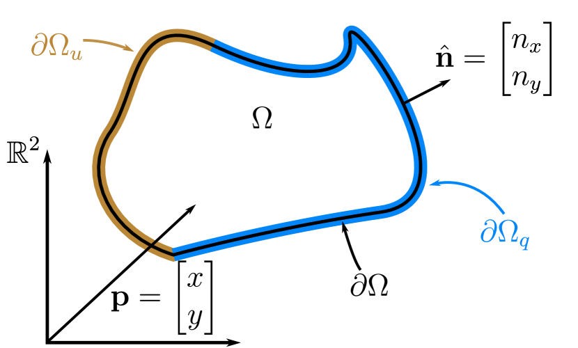
Figure 1: Graphical representation of an arbitrary two-dimensional (2D) domain $\Omega\subset\mathbb{R}^{2}$. A point within this domain is represented by $\mathbf{p}=(x,y)$. We define the boundary (a closed line, in this 2D example) as $\partial\Omega$, with local unit normal $\hat{\mathbf{n}}$. The boundary is partitioned into the Dirichlet boundary, $\partial\Omega_{u}$, and the Neumann boundary, $\partial\Omega_{q}$. The two boundaries do not intersect but span the entire boundary, i.e., $\partial\Omega_{u}\cup\partial\Omega_{q}=\partial\Omega$.

Within the context of heat transfer, Dirichlet boundaries are used to prescribe the temperature at a boundary, i.e., to create heat sinks. Neumann boundary conditions are instead suitable to prescribe the flux (i.e., the heat exchange) at a boundary. In Eq. (5), $\kappa$ is the same thermal conductivity term introduced earlier, and $\hat{\mathbf{n}}$ is a unit vector normal to the boundary (refer to Fig. 1). As we shall see later in Section II-F, our proposed FEM model uses Neumann boundary conditions to describe the heat convection that occurs on the tissue surface exposed to air and Dirichlet boundary conditions to model heat transfer where contacts occur.

II-B Derivation of the Weak Form

To derive the weak form of the problem, let us introduce an unknown, smooth function $w$ such that $w=0$ on the Dirichlet boundary $\partial\Omega_{u}$. In the FEM literature, $w$ is referred to as a weighting function. Multiplying both sides of Eq. (3) by $w$ and integrating over the domain, we obtain

$$\int_{\Omega}wc_{v}\frac{\partial u}{\partial t}dV=\int_{\Omega}w\nabla\cdot(\kappa\nabla u)dV+\int_{\Omega}wf(\mathbf{p})dV,$$ (7)

where $dV$ represents an infinitesimally small volume within $\Omega$. To ensure convergence of the integrals in Eq. (7), we require both $w$ and $u$ to have square-integrable first derivatives over $\Omega$. The equation above can be further rewritten by applying the divergence theorem and Green’s formula [23], yielding

$$\int_{\Omega}wc_{v}\frac{\partial u}{\partial t}dV+\int_{\Omega}(\nabla w)\cdot(\kappa\nabla u)dV=\\ +\int_{\Omega}wf(\mathbf{p})dV+\int_{\partial\Omega_{q}}wq_{n}dS.$$ (8)

Compared to Eq. (7), this new relation only contains first-order derivatives. Note that the last element on the right-hand side is a surface integral across $\partial\Omega_{q}$, i.e., the boundary on which we have imposed Neumann boundary conditions, with $dS$ representing an infinitesimal area on such surface. Throughout the remainder of this section, we illustrate how to numerically construct functions $w$ and $u$ that satisfy Eq. (8).

II-C Domain Discretization and Construction of the Solutions

Let us partition the spatial domain $\Omega$ into an arbitrary number of discrete subdomains (i.e., elements) $\Omega^{e}$, where $e=1,...,N_{el}$. While the shape and structure of the subdomains may be arbitrary, in this paper we shall consider cuboid elements with eight nodes per element, as illustrated in Fig. 2.

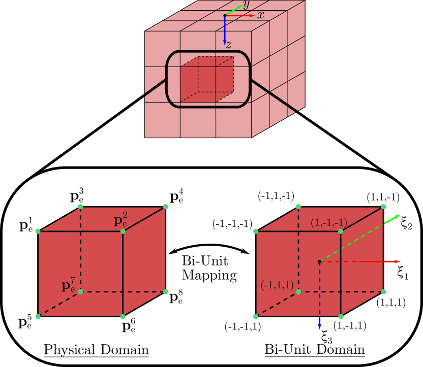
Figure 2: Domain discretization and bi-unit domain. Without loss of generality, here we assume tissue specimens to be shaped in the form of a cuboid, with a left-handed global frame on the top surface. The tissue geometry is partitioned into an arbitrary number $N_{el}$ of cuboid-shaped elements, each equipped with eight nodes. The coordinates of each node with respect to the global frame are denoted with $\mathbf{p}_{e}^{A}$, with the superscript $A$ identifying a specific node ($A=\{1,2,\ldots,8\}$). In the FEM method, candidate solutions for each element are built within a bi-unit domain, where local coordinates are bounded between $-1$ and $1$ along each axis. Eq. (10) provides a mapping between the physical domain and such bi-unit domain.

We define $u_{e}$ and $w_{e}$ as local approximations of $u$ and $w$ over $\Omega^{e}$. With these terms, Eq. (8) can be rewritten by summing the contributions from each element:

$$\sum^{N_{el}}_{e=1}\left[\int_{\Omega^{e}}w_{e}c_{v}\frac{\partial u_{e}}{\partial t}dV+\int_{\Omega^{e}}(\nabla w_{e})\cdot(\kappa\nabla u_{e})dV\right]=\\ \sum^{N_{el}}_{e=1}\left[\int_{\Omega^{e}}w_{e}f(\mathbf{p})dV+\int_{\partial\Omega_{q}^{e}}w_{e}q_{n}dS\right].$$ (9)

In FEM, $u_{e}$ and $w_{e}$ are built within a bi-unit domain (refer to Fig. 2), where a set of coordinates is represented by $\boldsymbol{\xi}=(\xi_{1},\xi_{2},\xi_{3})$ and coordinates are bounded between $-1$ and $1$ along each axis. The mapping between the bi-unit domain and the physical domain is given by

$$\mathbf{p}_{e}(\boldsymbol{\xi})=\sum_{A=1}^{N_{ne}}N^{A}(\boldsymbol{\xi})\mathbf{p}_{e}^{A},$$ (10)

where $N_{ne}=8$ is the number of nodes in the element and $N^{A}(\boldsymbol{\xi})$ are trilinear shape functions, i.e.,

$$N^{A}(\boldsymbol{\xi})=\frac{1}{8}(1+\xi_{1}^{A}\xi_{1})(1+\xi_{2}^{A}\xi_{2})(1+\xi_{3}^{A}\xi_{3}),$$ (11)

where $(\xi_{1}^{A},\xi_{2}^{A},\xi_{3}^{A})$ is the location of node $A$. With these definitions, we can finally construct candidate solutions $u_{e}$ and $w_{e}$ as

$$u_{e}=\sum_{A=1}^{N_{ne}}N^{A}(\boldsymbol{\xi})d^{A}_{e}=\mathbf{N}^{T}\mathbf{d}_{e}$$ (12)

$$w_{e}=\sum_{A=1}^{N_{ne}}N^{A}(\boldsymbol{\xi})c^{A}_{e}=\mathbf{N}^{T}\mathbf{c}_{e},$$ (13)

where $d^{A}_{e}$ and $c^{A}_{e}$ are nodal degrees of freedom. To approximate the temperature across the domain, it is necessary to calculate $\mathbf{d}_{e}$ for every element, as we show in the following section.

II-D Matrix-Vector Formulation

Using Eqs. (12) and (13), it is possible to obtain a more compact formulation for Eq. (9) which also is amenable to numerical implementation. Let us begin by considering the solutions $u_{e}$ and $w_{e}$ over a single domain element $\Omega^{e}$. Eq. (8) can be rewritten locally as

$$\int_{\Omega^{e}}w_{e}c_{v}\frac{\partial u_{e}}{\partial t}dV+\int_{\Omega^{e}}(\nabla w_{e})\cdot(\kappa\nabla u_{e})dV=\\ \int_{\Omega^{e}}w_{e}f(\mathbf{p})dV+\int_{\partial\Omega_{q}^{e}}w_{e}q_{n}dS.$$ (14)

Substituting Eqs. (12) and (13) into the relation above, we obtain

$$\int_{\Omega^{e}}\mathbf{c}_{e}^{T}\mathbf{N}c_{v}\mathbf{N}^{T}\dot{\mathbf{d}}_{e}dV+\int_{\Omega^{e}}(\nabla\mathbf{N}^{T}\mathbf{c}_{e})^{T}(\kappa\nabla\mathbf{N}^{T}\mathbf{d}_{e})dV=\\ \int_{\Omega^{e}}\mathbf{c}_{e}^{T}\mathbf{N}f(\mathbf{p})dV+\int_{\partial\Omega_{q}^{e}}\mathbf{c}_{e}^{T}\mathbf{N}q_{n}dS.$$ (15)

Note that the spatial derivatives and the integrals in Eq. (15) are expressed with respect to the global frame, whereas the shape functions used to construct $u_{e}$ and $w_{e}$ (i.e., Eq. (11)) were defined within the bi-unit domain. To correctly apply $\nabla$ to the shape functions, we need to apply the chain rule:

$$\nabla=J^{-T}\nabla_{\boldsymbol{\xi}},$$ (16)

where $\nabla_{\boldsymbol{\xi}}=\left(\frac{\partial}{\partial\xi_{1}},\frac{\partial}{\partial\xi_{2}},\frac{\partial}{\partial\xi_{3}}\right)^{T}$ and $J=\frac{\partial\mathbf{p}}{\partial\boldsymbol{\xi}}$ denotes the Jacobian matrix. Analogously, we change the bounds of integration from the element cuboid in the global reference frame to the cuboid in the bi-unit domain, where $dV=|J|dV^{\boldsymbol{\xi}}$. This allows us to rewrite Eq. (15) in a matrix-vector form:

$$\mathbf{c}^{T}_{e}\underbrace{\int_{\Omega^{e}_{\boldsymbol{\xi}}}\mathbf{N}c_{v}\mathbf{N}^{T}|J|dV^{\boldsymbol{\xi}}}_{\mathbf{M}_{e}}~{}\dot{\mathbf{d}}_{e}+\\ \mathbf{c}^{T}_{e}\underbrace{\int_{\Omega^{e}_{\boldsymbol{\xi}}}(J^{-T}\nabla_{\boldsymbol{\xi}}\mathbf{N}^{T})^{T}(\kappa J^{-T}\nabla_{\boldsymbol{\xi}}\mathbf{N}^{T})|J|dV^{\boldsymbol{\xi}}}_{\mathbf{K}_{e}}~{}\mathbf{d}_{e}=\\ \mathbf{c}^{T}_{e}\underbrace{\int_{\Omega^{e}_{\boldsymbol{\xi}}}\mathbf{N}\mathbf{N}^{T}\mathbf{f}_{e}|J|dV^{\boldsymbol{\xi}}}_{\mathbf{F}^{int}_{e}}+\mathbf{c}^{T}_{e}\underbrace{\int_{\partial\Omega^{e}_{q,\boldsymbol{\xi}}}\mathbf{N}q_{n}|J|dV^{\boldsymbol{\xi}}}_{\mathbf{F}^{q}_{e}}.$$ (17)

Note that we approximated $f(\mathbf{p})$ using the same trilinear shape functions used earlier to build $u_{e}$ and $w_{e}$, with nodal degrees of freedom $f^{1}_{e},...,f^{8}_{e}$.

We now aggregate local solutions to assemble global matrices:

$$\sum^{N_{el}}_{e=1}(\mathbf{c}^{T}_{e}\mathbf{M}_{e}\dot{\mathbf{d}}_{e}+\mathbf{c}^{T}_{e}\mathbf{K}_{e}\mathbf{d}_{e})=\sum^{N_{el}}_{e=1}(\mathbf{c}^{T}_{e}\mathbf{F}^{int}_{e}+\mathbf{c}^{T}_{e}\mathbf{F}^{q}_{e}),$$ (18)

which can be more compactly rewritten as

$$\mathbf{M}\dot{\mathbf{d}}+\mathbf{K}\mathbf{d}=\mathbf{F}.$$ (19)

In the equation above, $\mathbf{M}$ is the thermal mass matrix, $\mathbf{K}$ is the thermal conductance matrix, $\mathbf{F}$ is the heat source vector, and $\mathbf{d}$ is the tissue temperature at each node in the mesh. Note that Eq. (19) is equivalent to Eq. (9) but written as a linear ordinary differential equation. By solving Eq. (19) for $\mathbf{d}$, we can determine the temperature at any location in the mesh.

II-E Time Stepping

Equation (19) is a first-order differential equation that can be solved with discrete time stepping. Let us denote $\mathbf{d}_{n}$ and $\mathbf{v}_{n}$ to be the discrete approximations of $\mathbf{d}(t_{n})$ and $\dot{\mathbf{d}}(t_{n})$ respectively. This allows us to rewrite Eq. (19) as

$$\mathbf{M}\mathbf{v}_{n+1}+\mathbf{K}\mathbf{d_{n+1}}=\mathbf{F}_{n+1}.$$ (20)

Using the Crank-Nicolson method, we can define $\mathbf{d}_{n+1}$ as

$$\mathbf{d}_{n+1}=\mathbf{d}_{n}+\frac{\Delta t}{2}(\mathbf{v}_{n+1}+\mathbf{v}_{n}),$$ (21)

where $\Delta t$ is the duration of the time step. Substituting Eq. (21) into Eq. (20) and solving for $\mathbf{v}_{n+1}$ we get

$$\mathbf{v}_{n+1}=\left(\mathbf{M}+\frac{\Delta t}{2}\mathbf{K}\right)^{-1}\left(\mathbf{F}_{n+1}-\mathbf{K}(\mathbf{d}_{n}+\frac{\Delta t}{2}\mathbf{v}_{n})\right).$$ (22)

This expression defines $\mathbf{v}_{n+1}$ as only a function of $\mathbf{d}$ and $\mathbf{v}$ at the previous time step, $n$. We initialize $\mathbf{d}_{0}$ with the starting temperature of the mesh and $\mathbf{v}_{0}$ using Eq. (20). Then at each time step $n$, we first solve for $\mathbf{v}_{n+1}$ and then for $\mathbf{d_{n+1}}$.

II-F Boundary Conditions

In our model, we allow each element on the external surface of the domain to have one of three boundary conditions: a heat sink, constant flux, or convection boundary. In the case of a heat sink, we apply Dirichlet boundary conditions to the surface, restricting the temperature on the surface to some fixed value. For constant flux conditions, a Neumann boundary is applied to the surface and $q_{n}$ is set to the flux value. A special case of the flux boundary is a convection boundary, which models the heat transfer created by a fluid passing over a solid. We model such a flux using Newton’s Law of Cooling [24], i.e.,

$$q_{n}=h(T_{\infty}-u),$$ (23)

where $T_{\infty}$ is the temperature of the fluid and $h$ is the heat transfer coefficient.

III EXPERIMENTAL VERIFICATION

III-A Experimental Setup

To verify the accuracy of the proposed FEM model, we conducted laser-tissue interaction experiments using the setup shown in Fig. 3. A surgical carbon dioxide (CO${}_{\text{2}}$) laser, the Lumenis Acupulse (Lumenis, Yokneam, Israel) was used to irradiate soft tissue targets. The tissue surface temperature was recorded with an infrared thermal camera, the A655sc (Teledyne FLIR, Oregon, USA), and compared to the prediction generated by the FEM model.

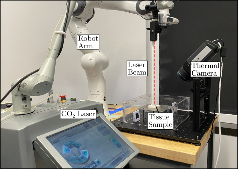
Figure 3: Experiments used a surgical CO${}_{\text{2}}$ laser whose beam is delivered through an articulated (passive) arm. The tissue surface temperature was monitored with an infrared thermal camera at a rate of 20 frames per second (fps), and spatial resolution of 70 $\frac{\text{pixel}}{\text{cm}}$. The distance between the beam’s focal point and the tissue surface ($d_{f}$) was controlled with a robotic arm.

In each experiment, the laser was applied for 15 seconds, and the tissue temperature was recorded for an additional 15 seconds in order to document cooling.

Two types of tissue targets were used in these experiments, namely ex-vivo chicken muscle, which was sourced from a local butcher shop; and agar-based gelatin, a soft tissue surrogate frequently used in thermal laser-tissue interaction studies [25]. The agar gels were fabricated in our laboratory using a mixture of 2% agar powder (Sigma-Aldrich Chemie, Germany) and 98% deionized water.

To further ascertain the generality of our model, we performed experiments with different levels of laser beam focusing. Intuitively, focusing the laser beam into a tighter spot will increase the beam intensity $I$, and it is expected to produce a stronger thermal response (refer to Eqs. (1) and (2)). In our experimental setup, the laser beam width $w$ is controlled by regulating the distance $d_{f}$ between the laser beam’s focal point and the tissue surface (see Fig. 3). The relation between $d_{f}$ and $w$ can be derived from simple laser optics [15]:

$$w(z)=w_{0}\sqrt{1+\left(\frac{\lambda(d_{f}+z)}{\pi w_{0}^{2}}\right)^{2}},$$ (24)

where $z$ is the optical axis of the beam, $\lambda$ is the laser wavelength, and $w_{0}$ is the beam waist (i.e., the radial width measured at the focal point). We conducted experiments with $d_{f}=\{25,30,35\}$ cm.

III-B FEM Simulation Setup

The FEM model described in Section II was implemented in C++ and compiled into a MEX file so that it could be run within the MATLAB environment (The MathWorks, Inc., Natick, MA, USA). The finite element mesh was initialized as a $(34\times 34\times 50)$ cuboid, representing a $(2\times 2\times 0.5)$ volume. The initial temperature of the cuboid was initialized to match the initial surface tissue temperature observed experimentally.

III-B1 Boundary Conditions

To model the heat exchange between the tissue specimen and the surrounding environment during each experiment, the FEM model was configured to use Dirichlet and Neumann boundary conditions. Specifically, a Dirichlet boundary was imposed on the bottom surface of the cuboid, to model a heat sink, representing contact between the tissue specimen and the underlying experimental bench. All remaining surfaces were treated as Neumann (i.e., convection) boundaries, given that they were fully exposed to air. We adopted a natural convection model [24], which involves using Eq. (23) and scaling the heat transfer coefficient $h$ by a value of $(T-T_{\infty})^{1/4}$. Here, $T_{\infty}$ denotes ambient temperature, which was measured with thermometers placed around the experimental setup. Observed values are reported in Table I.

III-B2 Tissue Physical Properties

In addition to the initial and boundary conditions, our FEM model requires knowledge of the tissue’s thermal and optical properties. Table I lists the parameters that were used by the simulator and their physical units.

TABLE I: FEM simulation parameters

Parameter	Agar	Chicken
$\mu_{a}$ ()	31	26
$c_{v}$ ()	4.3	3.73
$\kappa$ ()	0.0062	0.0049
$h$ ()	0.022	0.029
$T_{\infty}$ ()	24	24

The volumetric heat capacity and the thermal conductivity of the agar phantoms were calculated using the following empirical approximations from [18]:

$$c_{v} =(1.55+2.8w)\rho$$ (25)

$$k =0.0006+0.0057w,$$ (26)

where $w=0.98$ is the water content and $\rho=1.00$  is the material density. For the chicken muscle specimens, we assumed physical properties similar to that of human muscle tissue [26]. The absorption coefficient $\mu_{a}$ and heat transfer $h$ can be highly variable, thus making it impractical to use tabulated values from prior literature. Our approach for the selection of these two parameters was to manually tune them to reduce modeling error.

III-B3 Heat Source

The laser intensity $I$ was simulated based on the Lambert-Beer law [15]:

$$I=\frac{2P}{\pi w(z)}e^{\frac{-2}{w(z)}(x^{2}+y^{2})-\mu_{a}z}.$$ (27)

Here, $P$ is the laser power, $w$ is the beam’s radial width (which can be calculated based on Eq. (24)), and $x$, $y$, and $z$ are the coordinates of a Cartesian reference frame established on the tissue surface, whose $z$-axis corresponds to the optical axis of the laser beam.

III-C Results

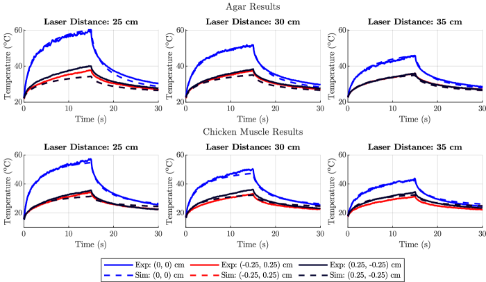
Figure 4: Simulated temperature results and experimental temperature results on agar tissue phantoms (top) and chicken muscle (bottom). The experimental results are the averages from the 5 trials for each combination of laser distance and tissue type.

Each experimental condition (two tissue types, three laser beam focusing levels) was replicated five times, for a total of 30 experimental runs. Results are shown in Fig. 4. Temperature profiles are shown for three locations on the tissue surface, i.e., the incidence point of the laser at $(0,0,0)$  and two locations located symmetrically around the incidence point at x- and y-coordinates $(-0.25,0.25)$  and $(0.25,-0.25)$ .

Average temperature tracking errors (root-mean-square error, RMSE) for each experimental condition are reported in Tables II and III. In most experimental conditions, the FEM model predicted the tissue temperature with a tracking accuracy within 2 . The largest observed RMSE was 3.31 .

TABLE II: Average Temperature RMSE (and Standard Deviation) for Experiments on Agar Specimens

Focal Distance $d_{f}$	25	30	35
Incidence Point	1.67 (0.31)	1.15 (0.19)	0.95 (0.12)
(-0.25, 0.25) cm	1.80 (0.68)	1.27 (0.59)	0.67 (0.10)
(0.25, -0.25) cm	3.31 (0.64)	1.80 (0.55)	0.63 (0.12)

TABLE III: Average Temperature RMSE (and Standard Deviation) for Experiments on Chicken Specimens

Focal Distance $d_{f}$	25	30	35
Incidence Point	1.53 (0.28)	1.62 (0.37)	1.27 (0.55)
(-0.25, 0.25) cm	2.15 (0.69)	1.59 (0.61)	2.18 (0.82)
(0.25, -0.25) cm	2.00 (0.81)	1.98 (0.30)	1.49 (0.74)

IV DISCUSSION

Experimental results show that the proposed FEM model can accurately predict the temperature of laser-irradiated tissue. This work addresses a gap in the current ecosystem of surgical robot simulators, laying the foundation for a new physics engine which will enable the integration of surgical lasers. Our model was validated through laser experiments on laboratory-made tissue phantoms and ex-vivo chicken muscle, achieving overall good tracking accuracy (see Fig. 4). While these results are promising, further work is needed to enhance the FEM model and integrate it in surgical robot simulators. While the model was verified on ex-vivo tissue, in-vivo tissue experiences additional cooling effects from perfusion (i.e., blood flow) [18]. Extending the model to account for perfusion may be necessary for accurate modeling in tissues with significant blood flow. Additionally, our model currently does not predict thermal tissue damage caused by laser heating. Incorporating the Arrhenius model [18] to calculate cellular death would enable the prediction of coagulation and other physical processes secondary to the heating. Another limitation of the present model is that it was only verified on tissue specimens having simple geometrical shapes. In the future, we plan to explore the generation of the tissue geometry for the FEM simulator based on medical imaging, analogously to the way in which Computer-Aided Design (CAD) software can generate meshes for Finite Element Analysis of complex parts. Finally, an analysis of the model’s computational complexity should be performed to evaluate its efficiency.

In general, the model produced more accurate predictions at the laser incidence point rather than surrounding areas. The most pronounced loss of accuracy was observed in the experiments with $d_{f}=25$ (observe the two leftmost plots in Fig. 4), where the laser spot was the tightest and thus produced the strongest thermal responses. This loss of accuracy may be due to the way convection cooling was implemented. Recall from section III-B1 that the simulation used a natural convection model, which scales the heat transfer coefficient $h$ by the difference between tissue and ambient temperature. While we take the temperature at a single location (i.e., the incidence point) to scale the heat transfer coefficient, the new value applies uniformly to the entire tissue surface. Therefore, cooler locations experience a stronger dissipation effect than they would if the heat transfer coefficient was scaled uniquely for each location. This effect could be mitigated by adjusting the simulation to have a unique heat transfer coefficient for every element in the mesh. Additional errors may arise from the modeling assumptions made throughout the manuscript. While we consider convective heat transfer, our model does not account for radiative heat transfer, which occurs at a rate proportional to the fourth power of temperature [24]. At higher temperatures, radiation may significantly cool the tissue. Furthermore, a tissue’s thermal and optical properties may vary during laser exposure due to temperature variations [18], but these values were held constant during the simulation. Lastly, our model neglects scattering and other nonlinear optical effects. These assumptions may be acceptable in first approximation [18] but may contribute to errors.

V CONCLUSION

This paper presented a Finite Element Method (FEM) model to simulate the thermal tissue response produced by surgical lasers. The model was validated through benchtop experiments on laboratory-made tissue phantoms and ex-vivo chicken muscle, achieving an RMSE generally smaller than 2 . These promising results lay the groundwork for the integration of surgical lasers into surgical robot simulators, which are currently not supported due to the lack of suitable physics engines.

Further work is necessary to enhance the proposed model’s applicability to real surgical scenarios. Specifically, extending the model to account for perfusion effects in in-vivo tissues is crucial for accurate thermal predictions, as blood flow can significantly influence tissue cooling. Additionally, incorporating the Arrhenius model to predict thermal tissue damage would enable the simulation of coagulation and other temperature-induced physical processes.

References

- [1] A. Attanasio, B. Scaglioni, E. De Momi, P. Fiorini, and P. Valdastri, “Autonomy in surgical robotics,” Annual Review of Control, Robotics, and Autonomous Systems, vol. 4, no. Volume 4, 2021, pp. 651–679, 2021.
- [2] G.-Z. Yang, J. Cambias, K. Cleary, E. Daimler, J. Drake, P. E. Dupont, N. Hata, P. Kazanzides, S. Martel, R. V. Patel, et al., “Medical robotics—regulatory, ethical, and legal considerations for increasing levels of autonomy,” Science Robotics, vol. 2, no. 4, p. eaam8638, 2017.
- [3] S. Schmidgall, A. Krieger, and J. Eshraghian, “Surgical gym: A high-performance gpu-based platform for reinforcement learning with surgical robots,” in 2024 IEEE International Conference on Robotics and Automation (ICRA). IEEE, 2024, pp. 13 354–13 361.
- [4] Q. Yu, M. Moghani, K. Dharmarajan, V. Schorp, W. C.-H. Panitch, J. Liu, K. Hari, H. Huang, M. Mittal, K. Goldberg, and A. Garg, “Orbit-surgical: An open-simulation framework for learning surgical augmented dexterity,” in 2024 IEEE International Conference on Robotics and Automation (ICRA), 2024, pp. 15 509–15 516.
- [5] P. M. Scheikl, B. Gyenes, R. Younis, C. Haas, G. Neumann, M. Wagner, and F. Mathis-Ullrich, “Lapgym - an open source framework for reinforcement learning in robot-assisted laparoscopic surgery,” Journal of Machine Learning Research, vol. 24, no. 368, pp. 1–42, 2023.
- [6] V. M. Varier, D. K. Rajamani, F. Tavakkolmoghaddam, A. Munawar, and G. S. Fischer, “Ambf-rl: A real-time simulation based reinforcement learning toolkit for medical robotics,” in 2022 International Symposium on Medical Robotics (ISMR), 2022, pp. 1–8.
- [7] A. Munawar, J. Y. Wu, G. S. Fischer, R. H. Taylor, and P. Kazanzides, “Open simulation environment for learning and practice of robot-assisted surgical suturing,” IEEE Robotics and Automation Letters, vol. 7, no. 2, pp. 3843–3850, 2022.
- [8] J. Xu, B. Li, B. Lu, Y.-H. Liu, Q. Dou, and P.-A. Heng, “Surrol: An open-source reinforcement learning centered and dvrk compatible platform for surgical robot learning,” in 2021 IEEE/RSJ International Conference on Intelligent Robots and Systems (IROS). IEEE, 2021, pp. 1821–1828.
- [9] E. Tagliabue, A. Pore, D. Dall’Alba, E. Magnabosco, M. Piccinelli, and P. Fiorini, “Soft tissue simulation environment to learn manipulation tasks in autonomous robotic surgery,” in 2020 IEEE/RSJ International Conference on Intelligent Robots and Systems (IROS), 2020, pp. 3261–3266.
- [10] A. Munawar and G. S. Fischer, “An asynchronous multi-body simulation framework for real-time dynamics, haptics and learning with application to surgical robots,” in 2019 IEEE/RSJ International Conference on Intelligent Robots and Systems (IROS), 2019, pp. 6268–6275.
- [11] G. A. Fontanelli, M. Selvaggio, M. Ferro, F. Ficuciello, M. Vendittelli, and B. Siciliano, “A v-rep simulator for the da vinci research kit robotic platform,” in 2018 7th IEEE International Conference on Biomedical Robotics and Biomechatronics (Biorob), 2018, pp. 1056–1061.
- [12] F. Faure, C. Duriez, H. Delingette, J. Allard, B. Gilles, S. Marchesseau, H. Talbot, H. Courtecuisse, G. Bousquet, I. Peterlik, and S. Cotin, SOFA: A Multi-Model Framework for Interactive Physical Simulation. Berlin, Heidelberg: Springer Berlin Heidelberg, 2012, pp. 283–321.
- [13] E. Coumans and Y. Bai, “Pybullet, a python module for physics simulation for games, robotics and machine learning,” http://pybullet.org, 2016–2021.
- [14] “GitHub - NVIDIAGameWorks/PhysX: NVIDIA PhysX SDK — github.com,” https://github.com/NVIDIAGameWorks/PhysX, [Accessed 29-10-2024].
- [15] H. C. Lee, N. E. Pacheco, L. Fichera, and S. Russo, “When the end effector is a laser: A review of robotics in laser surgery,” Advanced Intelligent Systems, vol. 4, no. 10, p. 2200130, 2022.
- [16] L. S. Mattos, A. Acemoglu, A. Geraldes, A. Laborai, A. Schoob, B. Tamadazte, B. Davies, B. Wacogne, C. Pieralli, C. Barbalata, et al., “ralp and beyond: Micro-technologies and systems for robot-assisted endoscopic laser microsurgery,” Frontiers in Robotics and AI, vol. 8, p. 664655, 2021.
- [17] L. Fichera, “Bringing the light inside the body to perform better surgery,” Science Robotics, vol. 6, no. 50, p. eabf1523, 2021.
- [18] M. H. Niemz, Laser-Tissue Interactions: Fundamentals and Applications. Springer International Publishing, 2019.
- [19] D. Pardo, L. Fichera, D. Caldwell, and L. Mattos, “Learning Temperature Dynamics on Agar-Based Phantom Tissue Surface During Single Point CO2 Laser Exposure,” Neural Processing Letters, vol. 42, no. 1, 2015.
- [20] D. Pardo, L. Fichera, D. G. Caldwell, and L. S. Mattos, “Thermal supervision during robotic laser microsurgery,” in 5th IEEE RAS/EMBS International Conference on Biomedical Robotics and Biomechatronics. IEEE, Aug. 2014, pp. 363–368. [Online]. Available: https://ieeexplore.ieee.org/document/6913803
- [21] A. Arnold and L. Fichera, “Identification of tissue optical properties during thermal laser-tissue interactions: An ensemble kalman filter-based approach,” International Journal for Numerical Methods in Biomedical Engineering, vol. 38, no. 4, p. e3574, 2022.
- [22] D. Marti, R. N. Aasbjerg, P. E. Andersen, and A. K. Hansen, “MCmatlab: an open-source, user-friendly, MATLAB-integrated three-dimensional Monte Carlo light transport solver with heat diffusion and tissue damage,” Journal of Biomedical Optics, vol. 23, no. 12, p. 1, Dec. 2018, publisher: SPIE-Intl Soc Optical Eng.
- [23] J. Fish and T. Belytschko, A First Course in Finite Elements. Chichester, England: John Wiley & Sons, Apr. 2007.
- [24] C. T. O’Sullivan, “Newton’s law of cooling—A critical assessment,” American Journal of Physics, vol. 58, no. 10, pp. 956–960, Oct. 1990. [Online]. Available: https://pubs.aip.org/ajp/article/58/10/956/1053575/Newton-s-law-of-cooling-A-critical-assessment
- [25] S. Rastegar, M. J. C. v. Gemert, A. J. Welch, and L. J. Hayes, “Laser ablation of discs of agar gel,” Physics in Medicine and Biology, vol. 33, no. 1, p. 133–140, Jan. 1988. [Online]. Available: http://dx.doi.org/10.1088/0031-9155/33/1/012
- [26] P. A. Hasgall, F. Di Gennaro, C. Baumgartner, E. Neufeld, B. Lloyd, M. C. Gosselin, D. Payne, A. Klingenbock, and N. Kuster. (2022, Feb) IT’IS database for thermal and electromagnetic parameters of biological tissues. [Online]. Available: itis.swiss/database