Approximate Constrained Lumping
Approximate Constrained Lumping of
Chemical Reaction Networks
Abstract
Gaining insights from realistic dynamical models of biochemical systems can be challenging given their large number of state variables. Model reduction techniques can mitigate this by decreasing complexity by mapping the model onto a lower-dimensional state space. Exact constrained lumping identifies reductions as linear combinations of the original state variables in systems of nonlinear ordinary differential equations, preserving specific user-defined output variables without error. However, exact reductions can be too stringent in practice, as model parameters are often uncertain or imprecise—a particularly relevant problem for biochemical systems.
We propose approximate constrained lumping. It allows for a relaxation of exactness within a given tolerance parameter , while still working in polynomial time. We prove that the accuracy, i.e., the difference between the output variables in the original and reduced model, is in the order of . Furthermore, we provide a heuristic algorithm to find the smallest for a given maximum allowable size of the lumped system. Our method is applied to several models from the literature, resulting in coarser aggregations than exact lumping while still capturing the dynamics of the original system accurately.
Keywords:
Approximate reduction Dynamical systems Biological models Constrained lumping1 Introduction
Biochemical models based on dynamical systems help discover mechanistic principles in living organisms and predict their behavior under unforeseen circumstances. Realistic and accurate models, however, often require considerable detail that inevitably leads to large state spaces. This hinders both human intelligibility and numerical/computational analysis. For example, even the relatively primary mechanism of protein phosphorylation may yield a state space that grows combinatorial with the number of phosphorylation sites [41].
As a general way to cope with large state spaces, model reduction aims to provide a lower-dimensional representation of the system under study that retains some dynamic properties of interest to the modeler. In applications to computational systems biology, it is beneficial that the reduced state space keeps physical interpretability, mainly when the model is used to validate mechanistic hypotheses [42, 46, 2]. There is a variety of approaches in this context, such as those exploiting time-scale separation properties [34, 58], quasi-steady-state approximation [43, 38], heuristic fitness functions [47], spatial regularity [53], sensitivity analysis [45], and conservation analysis, which detects linear combinations of variables that are constant at all times [55].
By lumping one generally refers to a reduction method that provides a self-consistent system of dynamical equations comprised of a set of macro-variables, each given as a combination of the original ones [aokiOptimizationStochasticSystems1967, kemenyFiniteMarkovChains1960, 34, 45]. In linear lumping, this reduction is expressed as a linear transformation of the original state variables. Since this can destroy physical intelligibility in general, constrained lumping allows restricting to only part of the state space by defining linear combinations of state variables that ought to be preserved in the reduction [31]. Lumping techniques of Markov chains date back to the early nineties [25]. These were later extended to stochastic process algebra [10, 59, 22, 49, 51], and have been expanded more recently to efficient algorithmic approaches for stochastic chemical reaction networks [11] and deterministic models of biological systems based on ordinary differential equations (ODEs) with polynomial right-hand sides [17, 15, 13].
In these cases, the reduction is a specific kind of linear mapping induced by a partition (i.e., an equivalence relation) of state variables; in the aggregated system, each macro-variable represents the sum of the original variables of a partition block. For polynomial ODE systems, CLUE has been presented as an algorithm that computes constrained linear lumping efficiently, i.e., in polynomial time [35], by avoiding the symbolic computation of the eigenvalues of a non-constant matrix that would have required in prior approaches [29, 31].
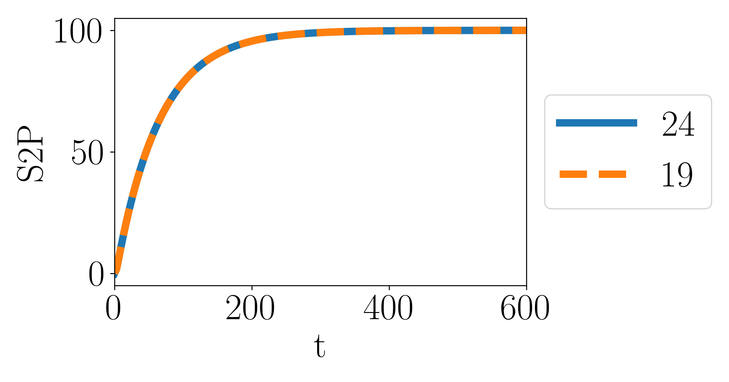
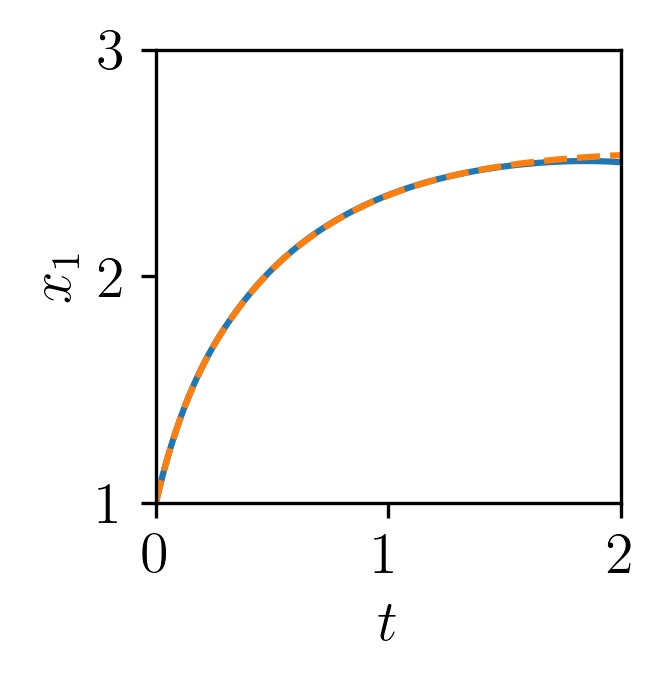
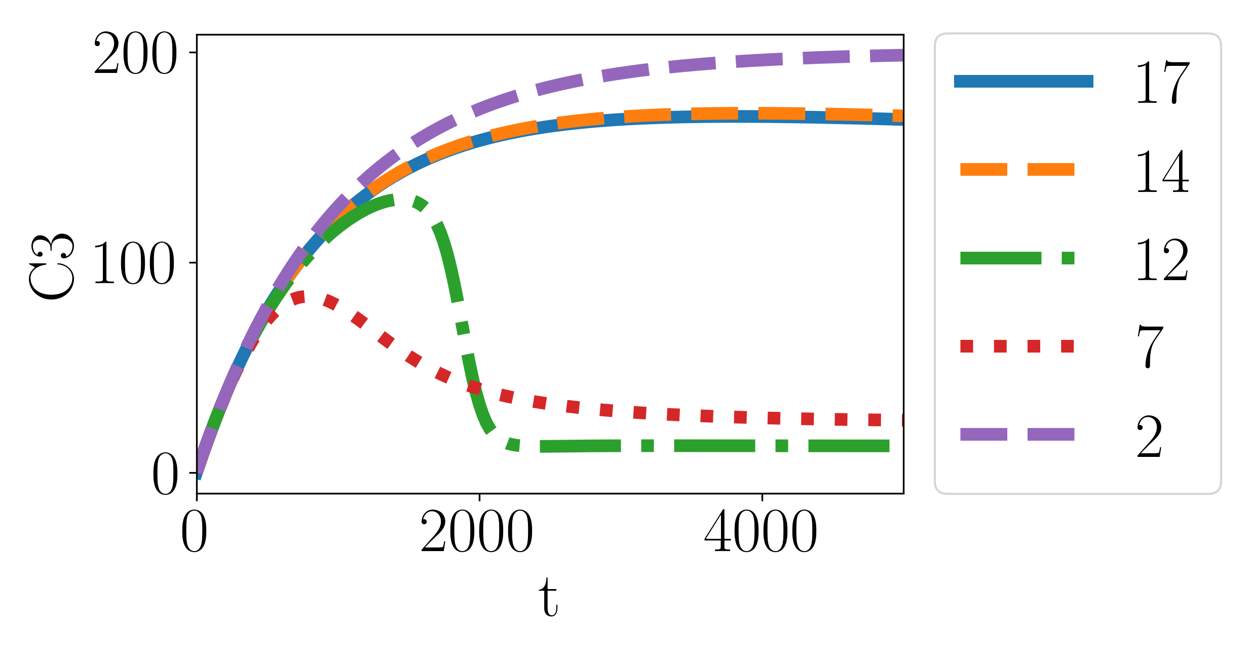
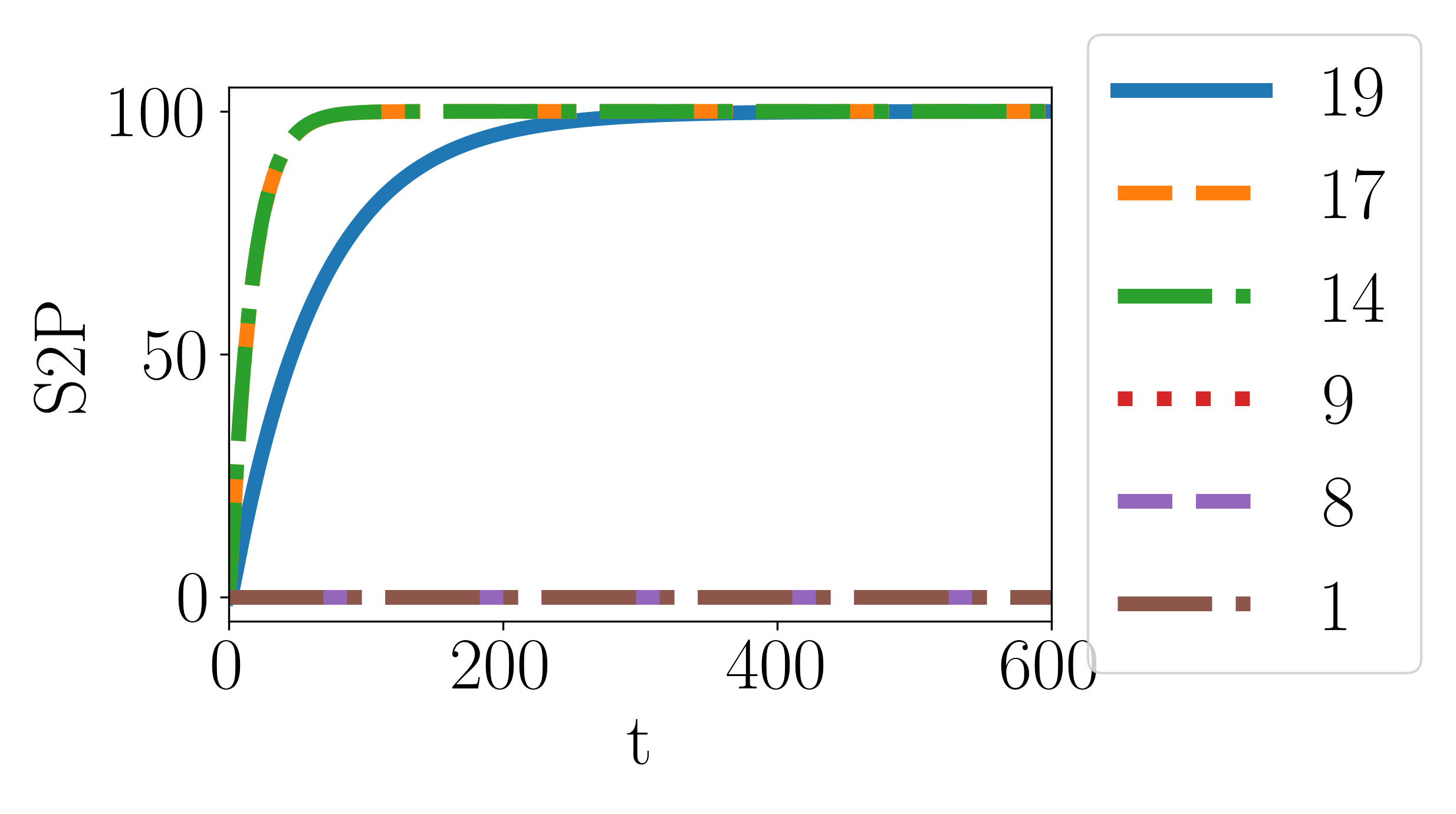
In particular, CLUE can compute the smallest linear dimensional reduction that preserves the dynamics of arbitrary linear combinations of original state variables given by the user. A complete step-by-step example of CLUE reduction on a synthetic 3-variables model is provided later (Exampe 1). To give a concrete example of the usefulness of CLUE applied to a real model, we consider a model of FceRI-like network of a cell-surface receptor [7]. The observable or quantity of interest is the amount of Phosphorylation at site Y2 (S2P), which is the sum of 10 out of the 24 variables in the model. Figure 1(a), displays the original simulation in blue and the orange line, instead, shows the solution of such observable on a model containing 19 variables obtained by reducing the former by CLUE. This plot shows that one can study the evolution of S2P using either the original model or one reduced by constrained lumping with only 19 variables without introducing any error.
All the aforementioned lumping approaches are exact, i.e., the reduced model does not incur any approximation error (but only loss of information because, in general, the aggregation map is not invertible). Approximate lumping is a natural extension that has been studied for a long time (e.g., [30]). Indeed, although exact reduction methods have been experimentally proved successful in a large variety of biological systems (e.g., [36]), approximate reductions can be more robust to parametric uncertainty—which notoriously affects systems biology models (e.g., [3, 5])—and offer a flexible trade-off between the aggressiveness of the reduction and its precision. This has been explored for partition-based lumping algorithms: In [16, cardelliFormalLumpingPolynomial2023], the authors present an algorithm for approximate aggregation parameterized by a tolerance , which, informally, relaxes an underlying criterion of equality for two variables to be exactly lumped into the same partition block. These approaches present notions of approximate reduction extending the above-mentioned exact reduction techniques for chemical reaction networks and ODEs. Similarly, in this paper, we present an extension of CLUE [35] that performs approximate constrained linear lumping of ODE systems. It relaxes the conditions for (exact) CLUE by introducing a lumping tolerance parameter that roughly relates to how close a lumping matrix is to an exact lumping. We consider ODE systems with analytical derivatives. These include rational and polynomial derivatives thus covering kinetic models for biochemical systems with Hill [57], Michaelis-Menten [57] and mass-action kinetics (e.g., [57, 50]).
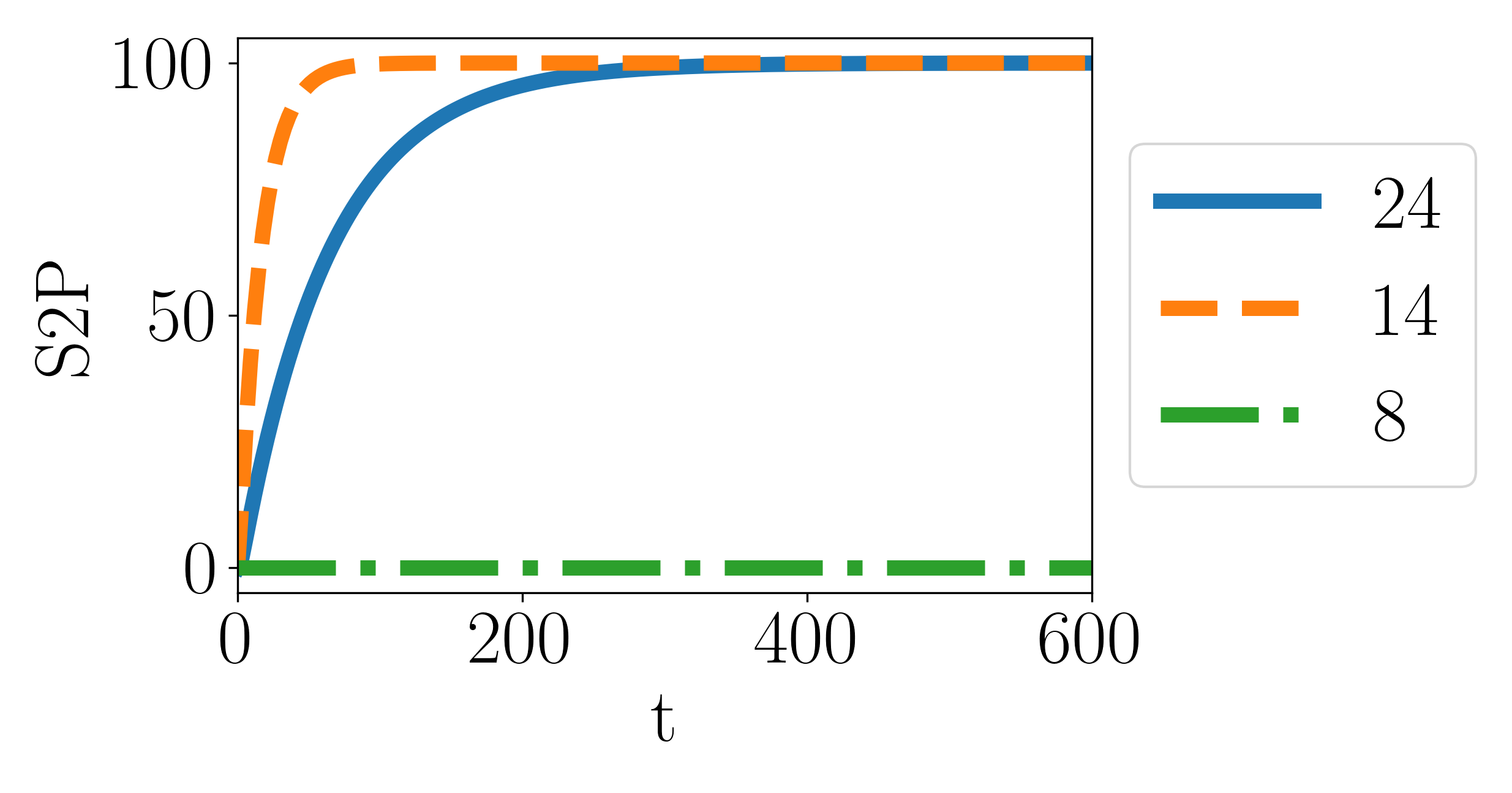
To obtain an approximate reduction for a given analytical ODE system, we start by finding a finite representation of the dynamics, either symbolically or using automatic differentiation [24]. Given a user-defined lumping tolerance, we can compute a reduced system that approximates the original one up to an error proportional to the lumping tolerance. For example, the orange line in Figure 1(b) shows that we can study the evolution of using an approximate reduction with 14 variables that yield the same steady-state value as in the original model. However, a too-permissive lumping tolerance may destroy the original dynamics, as shown by the approximate reduction with 8 variables (bottom green line).
Our proposed approach works in polynomial time. To find the lumping tolerance, we propose a heuristic approach based on the expected size of the reduced model. Using a prototype implementation, we evaluate the aggregation power of our approach on five polynomial models and three rational models representative of the literature. We also evaluate the scalability of our approach on a multisite phosphorylation model [44]. Overall, the numerical results show that our method can lead to substantially smaller reduced models while introducing limited errors in the dynamics.
This paper extends the conference paper [27] by expanding the theory to include analytical drifts; including models with rational drifts; adding a scalability analysis; and proposing a new approach to find the lumping tolerance. A short tool demonstration paper discussing implementation details of our approach has been recently presented in [cmsb2024_clue].
Further related work. We are complementary to classic works [30, 31] which do not address the efficient algorithmic computation of lumping. Moreover, we are more general than [23, 52, 16] which consider so-called “proper” lumping (i.e., [45]) where each state variable appears in exactly one aggregated variable. Likewise, we are complementary to rule-based reduction techniques [19] which are independent of kinetic parameters [12]. As less closely related abstraction techniques, we mention (bisimulation) distance approaches for the approximate reduction of Markov chains [4, 18] and proper orthogonal projection [1], which, however, apply to linear systems. Abstraction of chemical reaction networks through learning [39, 9] and simulation [21] are complementary to lumping.
Outline. Section 2 provides necessary preliminary notions. Section 3 introduces approximate constrained lumping, how to compute it, and how to choose the lumping tolerance value. Section 4 evaluates our proposal on models from the literature, while Section 5 concludes the paper.
Notation. For a function , we denote its domain by . The derivative with respect to time of a function is denoted by . We denote a dynamical system by , and denote its initial condition by . For , we denote the Jacobian of at by . Given a matrix , the rowspace of or the vector space generated by the rows of is denoted by . We denote by a pseudoinverse of (i.e. where is the identity matrix). We reserve the term rational for models with a non-trivial denominator on their right-hand side.
2 Preliminaries
In this paper, we study systems of ODEs of the form:
| (1) |
where and is an analytic function, for .
We first recall the notion of (exact) lumping [48]. Informally, it is defined as a mapping that leads to a self-consistent system of ODEs in the reduced state space.
Definition 1
Given a system of ODEs of the form given by Equation (1), and a full rank matrix with , we say that is an exact lumping of dimension (or that the system is exactly lumpable by ) if there exists a function with polynomial entries such that .
Example 1
Consider the following system
| (2) |
Then, the matrix
is an exact lumping of dimension 2, since
Definition 2
Given a system of ODEs of the form given by Equation (1), and an exact lumping , we say that are the reduced (or lumped) variables, and their evolution is given by the reduced system .
Given an initial condition and an exact lumping , there is a corresponding initial condition in the lumped variables given by . Similarly, since and , we have that
This means that we can study the evolution of the lumped variables by solving the (smaller) reduced system rather than the (larger) original one.
To answer whether it is possible to recover the evolution of some linear combination of state variables., we introduce the notion of constrained lumping.
Definition 3
Let for some matrix , for . We say that a lumping is a constrained lumping with observables if . This means that each entry of is a linear combination of the reduced variables .
Example 2
Suppose we are interested in observing the quantity where the evolution is given by the system (2). In this case with . We can see that from Example 1 is a constrained lumping as we can recover the observable from the reduced system, i.e., . Suppose now that we want to observe the quantity . In this case , thus matrix , is not a constrained lumping as it is not possible to obtain as a linear combination of and .
To understand how a constrained lumping can be computed, we first review the following known characterization of lumping.
Theorem 2.1 (Characterization of Exact Lumping [48])
Given a system of ODEs of the form given by Equation (1) and a matrix with rank , the following are equivalent.
-
1.
The system is exactly lumpable by .
-
2.
For any pseudoinverse of , .
-
3.
for all ; that is, the row space of is invariant under for all , where is the Jacobian of at .
The characterization of exact lumping in Theorem 2.1 provides us with a way to compute a constrained lumping . This is because, thanks to point 3, the problem of computing a lumping is equivalent to the problem of finding a -invariant subspace of for all . However, is a matrix whose entries are functions of . In other words, there is a different real-valued matrix for each . To circumvent this issue, we require the following result:
Theorem 2.2 ([24, Lemma 1])
A set of matrices can be found analytically when can be represented as
| (3) |
where is a set of analytic functions. When working with polynomial systems, each of the entries of is a polynomial and so each corresponds to the monomials of .
For instance, for rational systems, can be obtained symbolically by differentiating and then multiplying by the minimum common denominator (mcd) of all entries of . In practice, this approach is computationally unfeasible since this symbolic approach results in an explosion of the number of monomials in . To avoid any explicit symbolic computation, a representation can be obtained by sampling at different points and using automatic differentiation [24, Section 3.4]. The general idea of this sampling procedure is formalized by Algorithm 1. In [24], the authors argue that a uniform sampling of values finds almost surely .
Example 3
Consider the system from Example 1. Before finding a basis for using the sample-based approach, we exemplify the symbolic approach to display its complexity. It starts by symbolically differentiating to obtain :
We then find the mcd of all entries of , which is . Since is rational in all its entries, it follows that , where is a matrix with polynomial entries up to degree 5. Notice that to obtain a monomial representation of , we need to expand all its terms.
We see that Algorithm 1 outputs a set of matrices spanning . Given such a set, Theorem 2.2 provides an algorithmic way to find a constrained lumping by performing a finite number of checks over real-valued vectors. This is shown in Algorithm 2. The use of Algorithms 1 and 2 to obtain a constrained lumping is summarized in Algorithm 3.
3 Constrained Approximated Lumping
This section introduces the formal theory underlying approximate constrained lumping, as well as its computational aspects. In Section 3.1 we present the definition of approximate constrained lumping. We introduce the deviation tolerance , which relaxes the conditions for lumping granting additional aggregation power. We prove how the error bound depends on the deviation tolerance. Next, we focus on how to compute an approximate constrained lumping. In Section 3.2 we introduce a numerical lumping tolerance to compute a lumping matrix and show how it relates to the deviation tolerance. In Section 3.3, instead, we discuss how to pick an appropriate value for the lumping tolerance in a way that leads to satisfactory results for both polynomial and rational systems.
3.1 Definition and error estimation
We begin by demonstrating why the condition for exact lumping can be too restrictive for finding reductions. Consider the following system of ODEs:
| (4) |
Notice that the system given by Equation (4) is similar to that of Equation (2), as we have just added a term to the numerator of its first equation. While the initial system is lumpable by , this new system is not exactly lumpable by . However, we would like to know if it is still possible to use the matrix to obtain a useful reduced system that approximates well the original one. To do so, we first want to evaluate how close the matrix is to (i.e., how much it deviates from) an exact lumping.
By Theorem 2.1, Point 2, a full rank matrix is a lumping if and only if the equality is satisfied for all , where denotes the domain of . In our proposal of approximate lumping, we relax this requirement by asking it to be satisfied up to a certain tolerance.
Definition 4
Consider the system of ODEs in Equation (1). Let be a full rank matrix with and denote by the Moore-Penrose pseudoinverse of and by the orthogonal projection operator onto . We define the deviation of at by
| (5) |
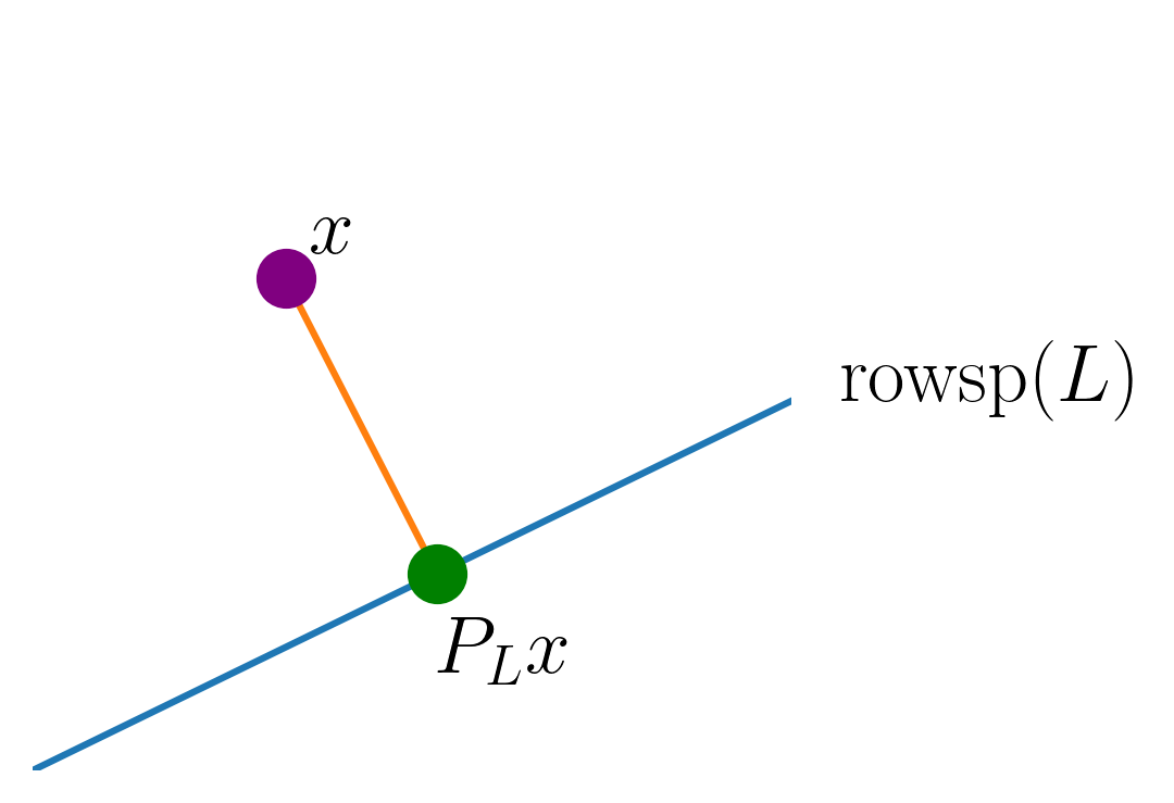
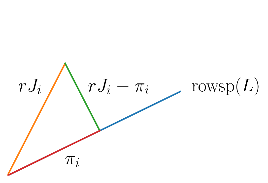
To understand the intuition behind Definition 4, consider the point in Figure 2. Then, the deviation computes the difference between the images under of (purple) and (green). The deviation is identically zero if and only if is a lumping.
Example 4
Consider the matrix given in Example 1. A pseudoinverse of is given by . Writing for the corresponding vector field, we obtain that , as is an exact lumping. Now consider the system given by Equation (4) and use to denote the corresponding vector field. Then, we get that . Therefore, the matrix is not an exact lumping of Equation (4).
From a modelling perspective, a reduced model is meaningful insofar as its predictions for a set of initial conditions of interest are close enough to those of the original model throughout a given finite time horizon. While the theory in [35, 24] guarantees that reduced models provide exact predictions, this might restrict the actual aggregation power of the technique. We aim to relax this theory by considering reductions that need not be exact or tight. Having this in mind, we introduce the following notion.
Definition 5
Consider the ODEs from Equation (1), a set of initial conditions , and a finite time horizon such that is well-defined on for all initial conditions . Given a full rank matrix and , we say that Equation (1) is approximately lumpable by with deviation tolerance if
| (6) |
for all . We say that is an approximate lumping for the set , time horizon , and with deviation tolerance (or -lumping). We will omit , or whenever they can be inferred from the context.
Remark 1
In practice, modellers often use biological models to study the evolution of a system for a fixed set of initial conditions and a time horizon . The assumption is that the behaviour of interest to the modeler occurs within time .
Example 5
After having generalized the notion of lumping to approximate lumping, we next introduce approximate constrained lumping in an obvious manner.
Definition 6
Let for some matrix with . We say that an approximate lumping of Equation (1) is an approximate constrained lumping with observables if .
Similarly to Definition 2, Definition 6 means that the observables can be recovered as a linear combination of the reduced variables .
Definition 7
The reduced system induced by an approximate lumping is given by , where .
Example 6
Definition 8
Example 7
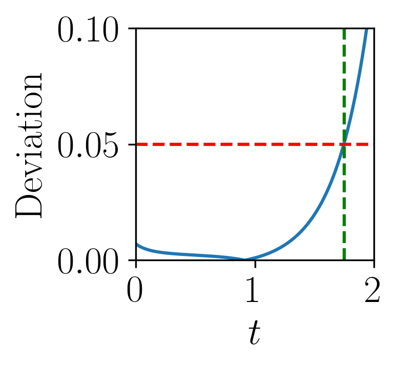
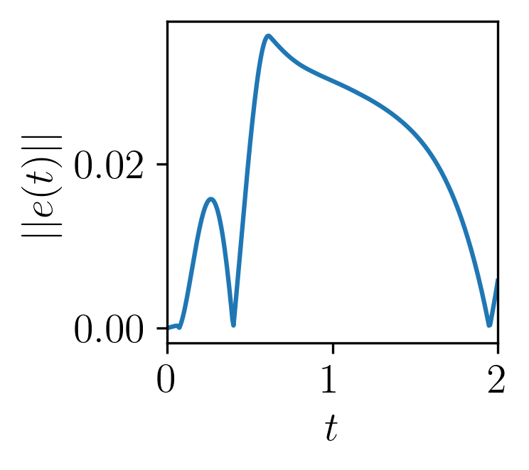
Following Example 6, we compute the trajectories of the reduced and original systems. We also compute the -error of the reduction. This is summarized in Figure 4. Note that, in this example, we obtained a reduction of a system that was not exactly lumpable. In Figure 4(a), we can appreciate that, for the given time horizon, the reduced and original values are close to each other.
We next show that it is possible to bound the error introduced by approximate constrained lumping. Even though our worst-case bound is often conservative in practice, the bound confirms the consistency of the approach: the error is of order — that is, the actual error decreases linearly with the deviation . Moreover, as we will see in Section 4, our framework can find approximate lumpings with low errors for published biological models.
Theorem 3.1 (Error Bounds)
Fix a bounded set of initial conditions , a finite time horizon and assume that the respective reachable set of the -dimensional ODE system is bounded on . If there exists a compact set such that for all and all and is analytic in , then for any for which is a lumping, it holds that , where
Here, is the Lipschitz constant of over the set of initial conditions .
3.2 Lumping Algorithm
In this section we relax the condition in Line 5 of Algorithm 2, thus allowing us to find approximate reductions. Intuitively, we add a new row to the matrix only if it is far enough from . We make this rigorous by fixing a lumping tolerance and adding a row only if , where is the orthogonal projection of onto . Thus, we propose Algorithm 4.
Remark 2
In Line 7 of Algorithm 4 we do not append , given by the orange vector in Figure 5. Rather, we append the normalized component of in the orthogonal direction to , which is , the green vector in Fig. 5. This ensures that the matrix is orthonormal. We can use the fact that the pseudoinverse of an orthonormal matrix is its transpose to obtain that .
We now provide a detailed example of Algorithm 4.
Example 8
Consider the system given by Equation (4) and let . Set i.e., we are observing the component from the original system. Using Algorithm 1 with the same points as in Example 3, we find that the dimension of is 6 with basis given by the matrices:
We begin the computation in Line 2 by setting and begin the main loop in Line 4 with . To carry out the computation of Line 5, we have that
Let . By the check of Line 6, we do not append any new row to as since . Next, we compute following Line 5. As , it follows that , which, by Line 6, means that we need to append a new row to . By Line 7, we add normalized as a row of (Line 7), thus obtaining
| (7) |
Going back to Line 5 with the updated matrix , we compute . Following Line 6, we do not add additional rows to since . We compute and , leaving unchanged. We go on with the computations for the remaining matrices to obtain . It follows that we need not add any new rows to .
So far we have only checked the first row of . Following the main loop (Line 4), we set . We compute
We continue computing , , while for . It follows that the check of Line 6 is false for all ; meaning that no more rows should be added to , thus terminating the algorithm. The output of Algorithm 4 is the matrix of Equation (7).
The following result states that approximate constrained lumpings can be efficiently computed.
Theorem 3.2 (Time Complexity of Algorithm 4)
Approximate constrained lumping can be computed in polynomial time. Specifically, the complexity of Algorithm 3 when using Algorithms 1 and 4 as subroutines can be bounded by , where is the cost of computing an entry of , is the dimension of , is the number of matrices spanning , and is the dimension of the reduced system.
When the system is not approximately lumpable, it follows that the worst-case time complexity is . The complexity bound of Theorem 3.2 can be further improved by using more efficient data structures [35].
The next result relies on Theorem 2.2 and ensures that the approximate reductions found by Algorithm 4 admit a deviation tolerance of order . In other words, the deviation tolerance is in the order of the lumping tolerance .
Theorem 3.3 (Correctness of Algorithm 4)
Using the setting of Theorem 3.1, assume can be written in the form given by Equation (3). Let be the matrix computed via Algorithm 4 with lumping tolerance over the sampled matrices for . Then, is a -lumping, where , is a constant depending on the representation of and is a constant depending on the trajectories and .
3.3 Heuristic search of lumping tolerance
To apply Algorithm 4, it is important to choose an appropriate value for . While Theorems 3.1 and 3.3 allow for an error estimation in terms of , in practice, this bound is not tight enough. For this reason, we introduce a heuristic approach to appropriately choose .
Intuitively, by increasing , it is possible to lump more variables together at the price of larger approximation errors. We would like to find the largest admissible such that the approximation error is small enough. To this aim, we begin by noting that the minimum value that can have is , corresponding to an exact reduction. A naive idea would be to set and add small increments until the reduction is satisfying. However, this requires an appropriate choice of increment which in turn depends on the model. Instead, Lemma 1 gives us an upper bound for which can be computed for each model.
Lemma 1 (Upper bound on )
Consider a matrix of observables of rank with th row denoted by and a decomposition of the Jacobian . Let be given by
| (8) |
for and each , where is the projection onto . Then is the smallest such for any the output of Algorithm 4 will be a matrix of orthonormal rows spanning the row space of .
Lemma 1 states that any will collapse the dynamics of the system onto observable . In this way, for any given model, we have a range from which to choose the right value for .
Remark 3
The value of depends not only on the chosen model and observable but also on the set of matrices used to represent . Compared to polynomial models, the values for the drift in rational models can be more sensitive to changes in , especially when the denominator of is close to . This sensitivity can be explained by vanishing denominators in the Jacobian of a rational drift . We therefore expect rational models to exhibit larger fluctuations of .
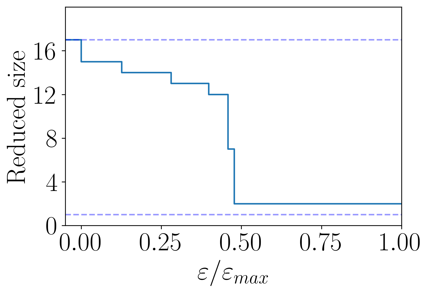
For example, the evolution of the reductions for different values of is demonstrated for a model from the literature in Figure 6. The model, named BIOMD103, has been downloaded from the online repository ODEbase [32] discussed in greater detail in Section 4 (it is model 2 from Table 1).
We note that previous work [27] used the deviation as a proxy to estimate the error without having to simulate the original system. This approach relied on a Monte Carlo approximation of the norm of over , where is the center of the initial set. While being effective in finding meaningful reductions for polynomial systems, this deviation-based approach can be problematic for rational systems. This is because rational systems are more sensitive to the choice of compactum, since a small change in the denominator can have a large effect on the overall value of , especially for values of where the denominator approaches .
We propose a novel approach which gives satisfactory results for both polynomial and rational systems (Section 4). Using the fact that the size of a reduced model decreases monotonically with , we set up a target (a cutoff size, ) for the reduced model given as a percentage of its original size. We then apply a binary search algorithm to find the largest such that the reduced model’s size satisfies . In terms of Figure 6, we want to obtain the smallest whose induced size is below the cutoff size. This intuition is formalized by Algorithm 5.
Remark 4
It is important to notice that the choice of minimal different in Algorithm 5 provides a trade-off between detecting reductions and the speed of the approach. A lower value for can lead to finding more reductions at the cost of more iterations.
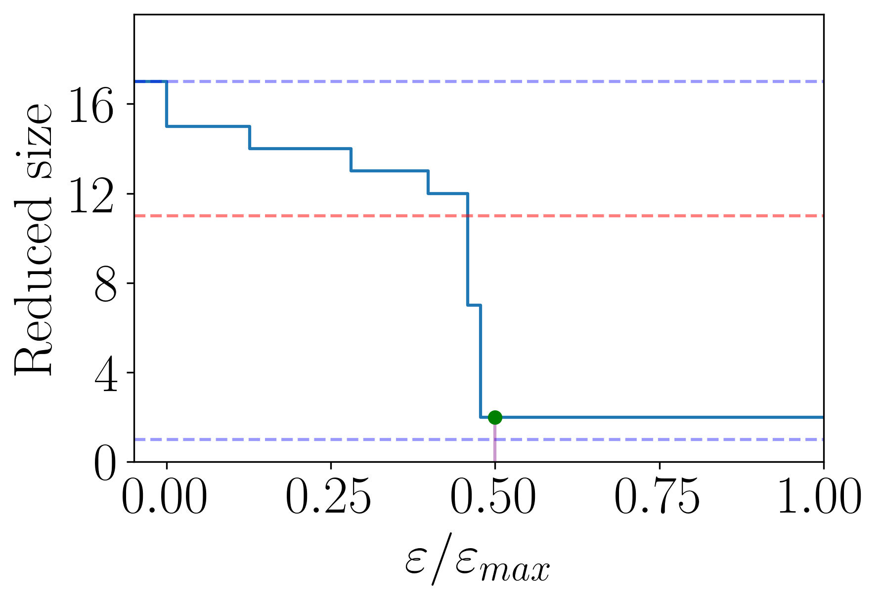
Example 9
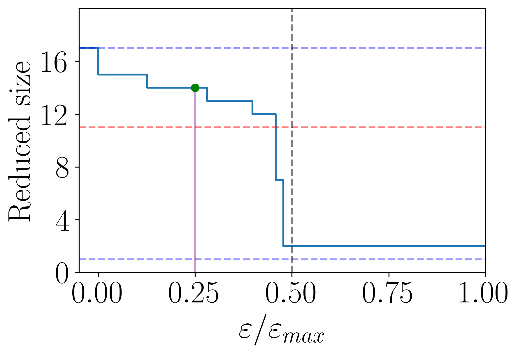
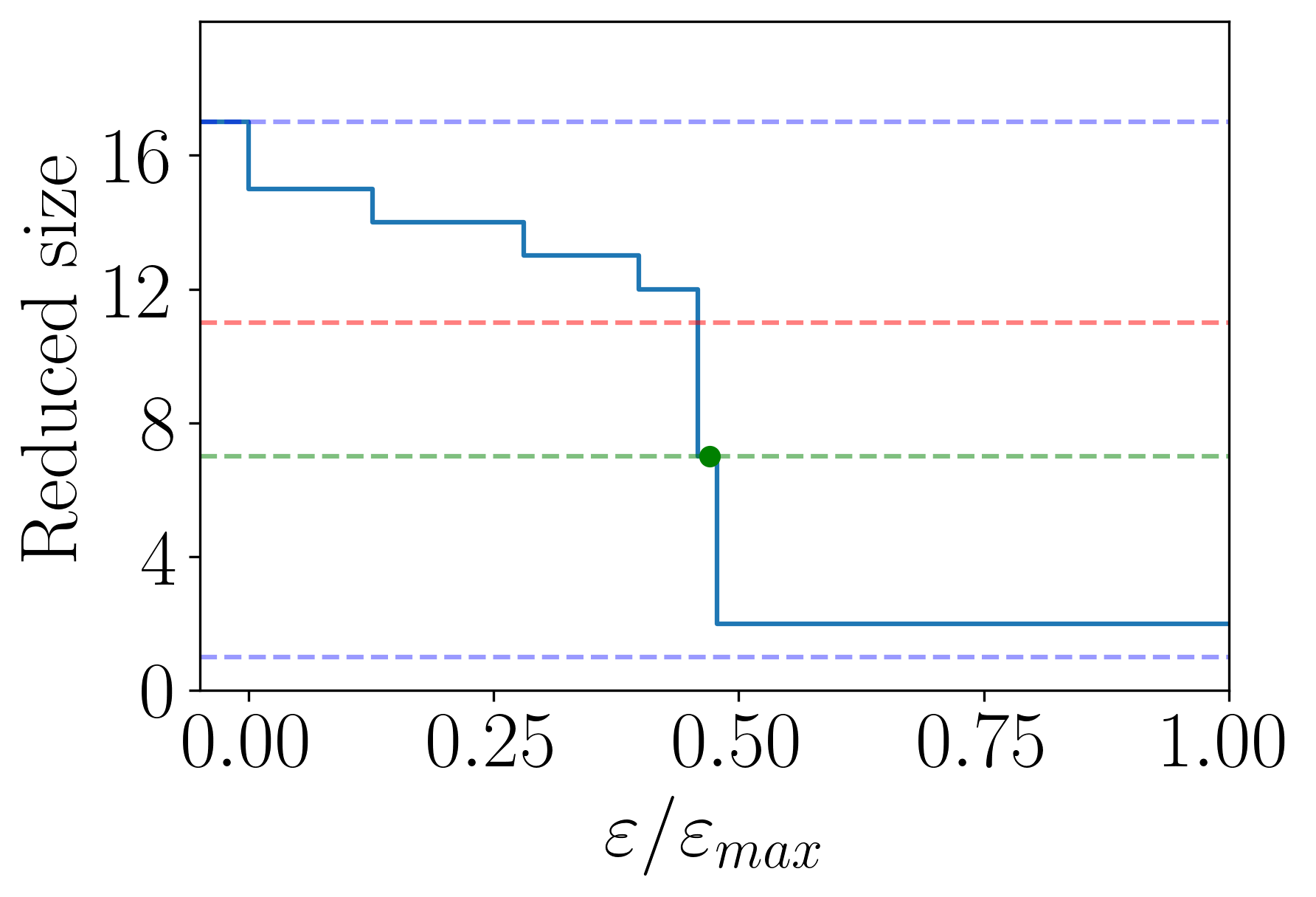
Let us use again model BIOMD103 from Figure 6. It has an observable of interest, [26], consisting of one variable representing the concentration ofActivated capsase3. We would like to find a reduction such that the reduced model size is at most of the original size (), i.e., species. To do so, we use Algorithm 5. We first verify (Line 3) that the cutoff size is larger than the minimum size and smaller than the size of the exact reduction. As the cutoff size is between and we continue to Line 8. On the first iteration (Figure 7(a)) the middle point (green) gives a reduction of size . As this size is smaller than the goal size , we set . This gives a new interval to search for a reduction (black line on Figure 7(b)). We continue following the algorithm until it converges to a reduction of size (green line Figure 7(c)). This is a correct result as we can see that the closest step below the cutoff size is the one of size in Figure 7(a).
4 Evaluation
In this section, we evaluate our method. All experiments were performed using an extension of the tool for CLUE [35, 24, cmsb2024_clue], an open-source Python library. The experiments are available in the following repository.
https://github.com/clue-developers/CLUE/releases/tag/v1.7.3
In Section 4.1, we use a selection of models from the literature to show how our approach can lead to small reductions while not incurring a large error. In Section 4.2, we use a perturbed multisite protein phosphorylation model to show the scalability of our approach.
4.1 Reduction power
To evaluate the reduction power of our approach, we selected several models from the literature. These models are chemical reaction networks with or more species. We used two sources to select models. The first is a collection of polynomial models from the literature written in the input format of the tool BioNetGen [6]. We selected two such models. The second is the so-called ODEbase project [32] which offers importing/exporting capabilities for polynomial and rational models from the BiomodelsDB repository [28]. We selected six such models. Models with prefix BIOMD were taken from ODEbase, while the remaining models were taken directly from the supplementary material of their original paper. For each model, the observable was chosen according to the observables studied in the original paper describing the model. These typically consist of one variable or linear combinations of them. For models where more than one observable was studied in the original paper, we arbitrarily selected one of them. Models written in the BioNetGen format were first imported by ERODE [14], our tool that collects many techniques for the reduction of biological systems, and then exported in ERODE’s .ode format supported by CLUE.
To import models from the ODEbase project [32], instead, we directly implemented in CLUE an importer to convert them in .ode format.
When available, the set of initial conditions necessary for simulations was taken from the original paper or the model files in BiomodelsDB [28]. The time horizon was either taken from the original reference or chosen experimentally by noticing when steady state was reached. All this additional information was manually added to the .ode files to the corresponding model.
When choosing the models, we aimed for a selection that could equally display our approach for both rational and polynomial models. The final selection of models is displayed in Table 1. The column Type reports whether the model is polynomial (P) or rational (R).
The source paper presenting the model is displayed in the Ref. column. The column Description contains a summary of the biological system studied in the model. In column Observable, we can see the species (or linear combinations of them) chosen as a constraint for the lumping. Finally, column Size displays the number of model variables added in the observable over the total number of variables in the system (e.g., in Model 5, S2P sums 10 out of the 24 variables of the model).
| Nr. | Name | Type | Ref. | Description | Observable | Size |
|---|---|---|---|---|---|---|
| 1 | BIOMD102 | P | [26] | Signaling pathways involved in the initiation of apoptosis (wild-type model) | Activated capsase3 (C3) | 1/12 |
| 2 | BIOMD103 | P | [26] | Signaling pathways involved in the initiation of apoptosis (competitive model) | Activated capsase3 (C3) | 1/17 |
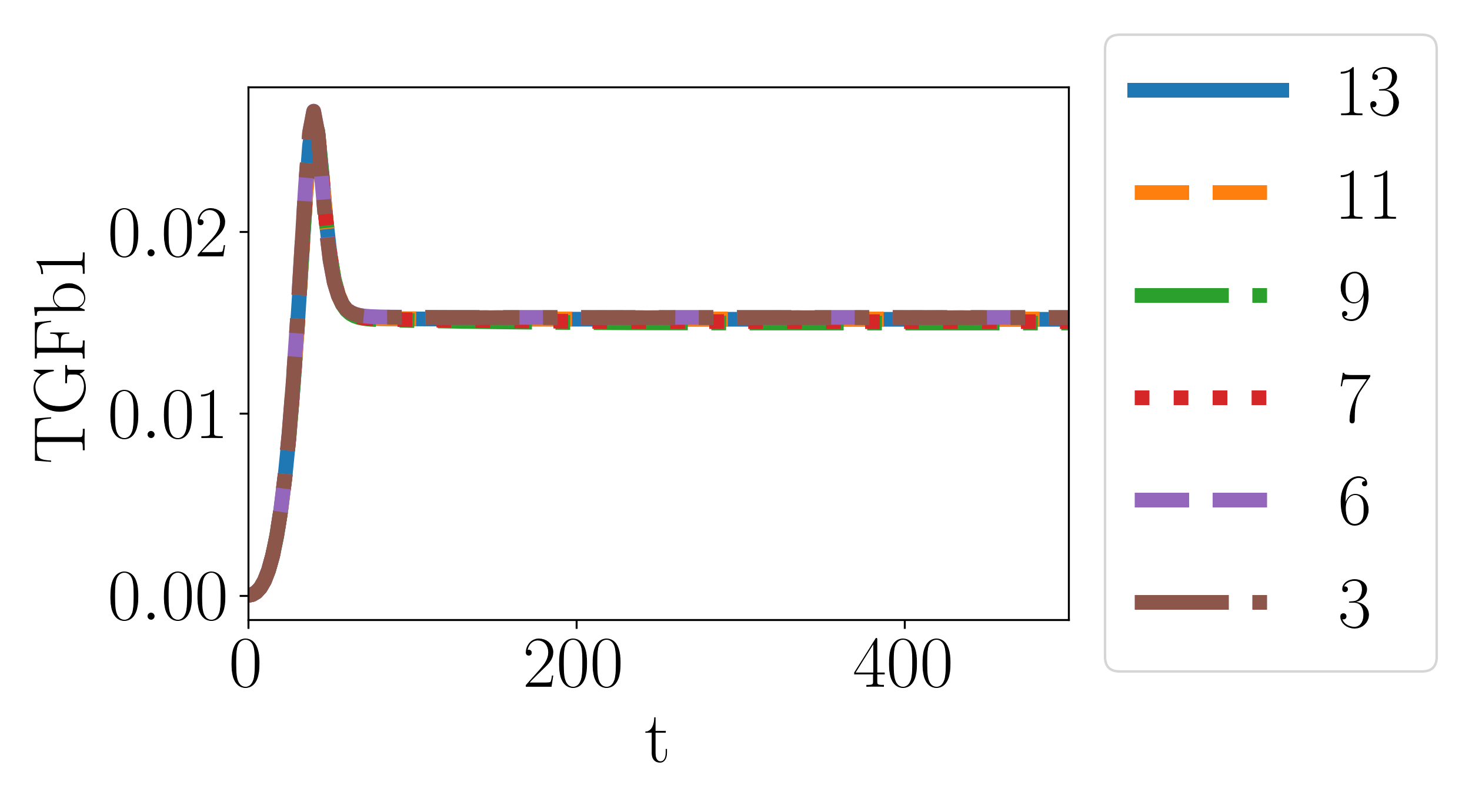
| 3 | BIOMD447 | P | [56] | Thrombospondin-Dependent Activation of TGF-1 | Transforming growth factor (TGF)-1 (TGFb1) | 1/13 |
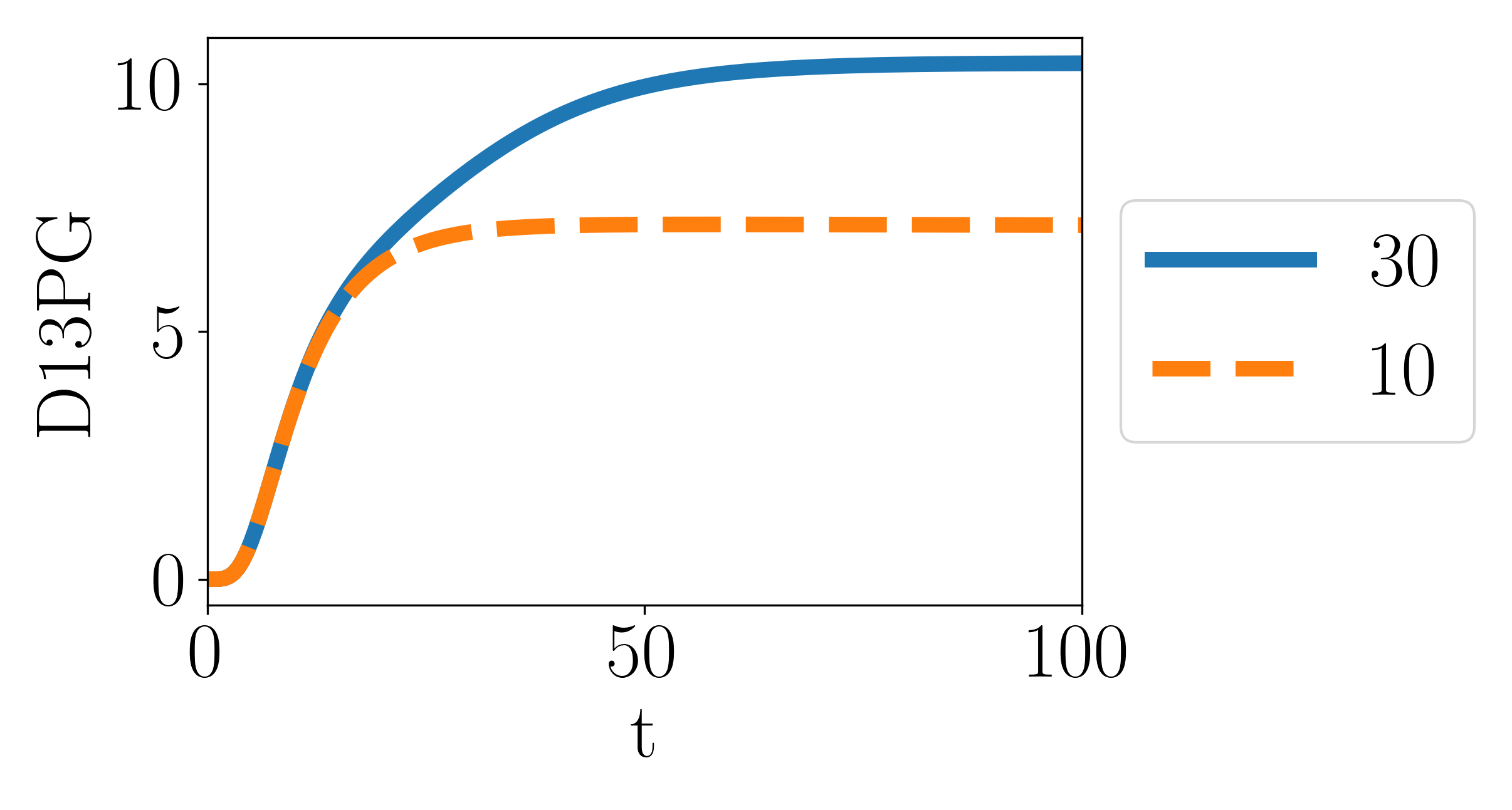
| 4 | BioNetGen_CPP | P | [33] | Central carbon pathway of E. coli | 1,3-diphosphoglycerate (D13PG) | 2/87 |
| 5 | NIHMS80246_S6 | P | [7] | FceRI-like network of a cell-surface receptor | Phosphorylation at Y2 (S2P) | 10/24 |
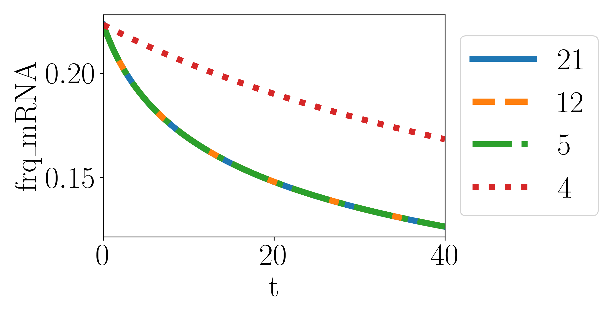
| 6 | BIOMD437 | R | [54] | Circadian clock of the fungus Neurospora crassa | Frequency of (frq_RNA) | 1/39 |
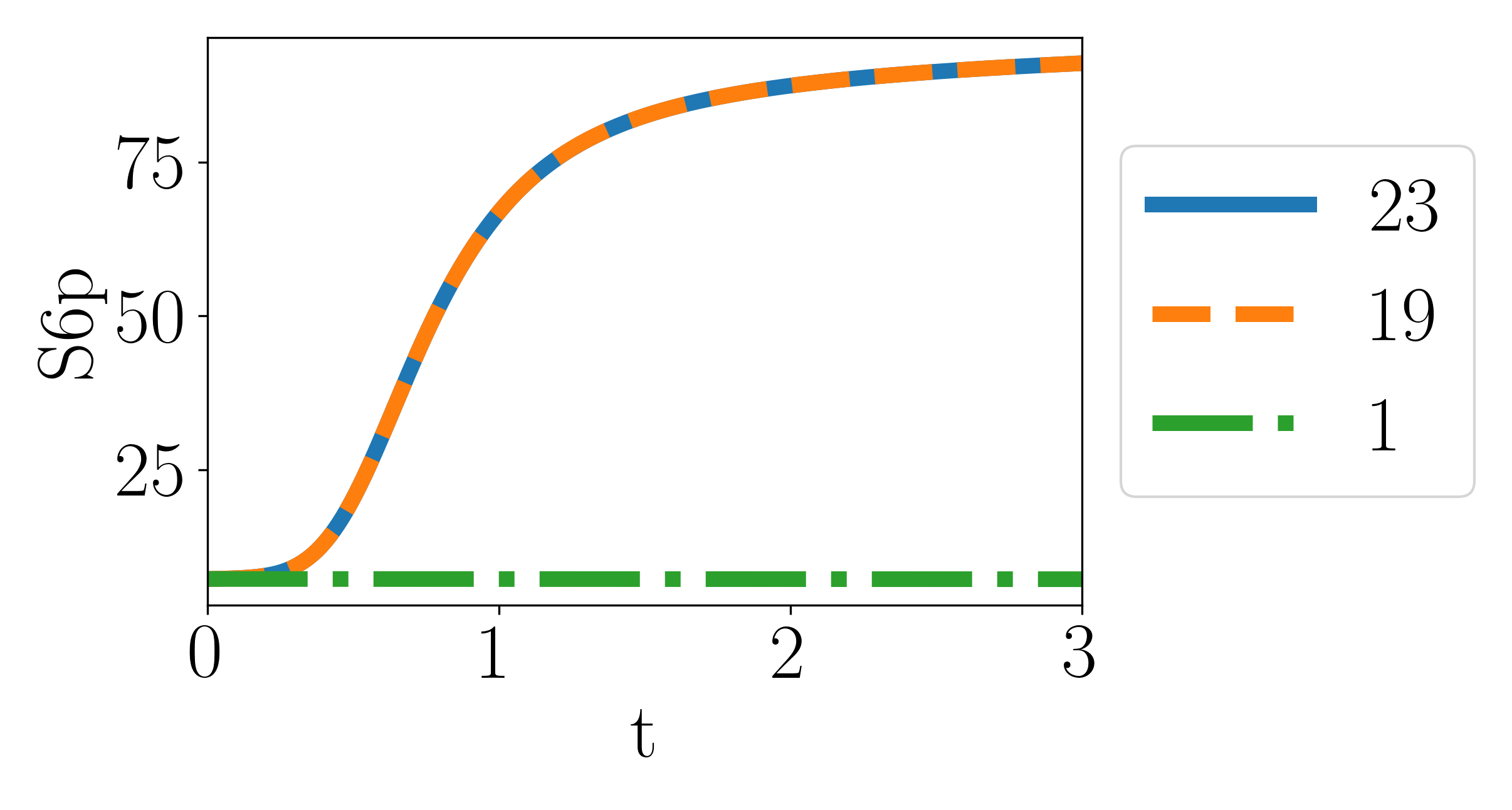
| 7 | BIOMD448 | R | [8] | Insulin Signaling in Type 2 Diabetes | Phosphorylation of site S6 (S6P) | 1/23 |
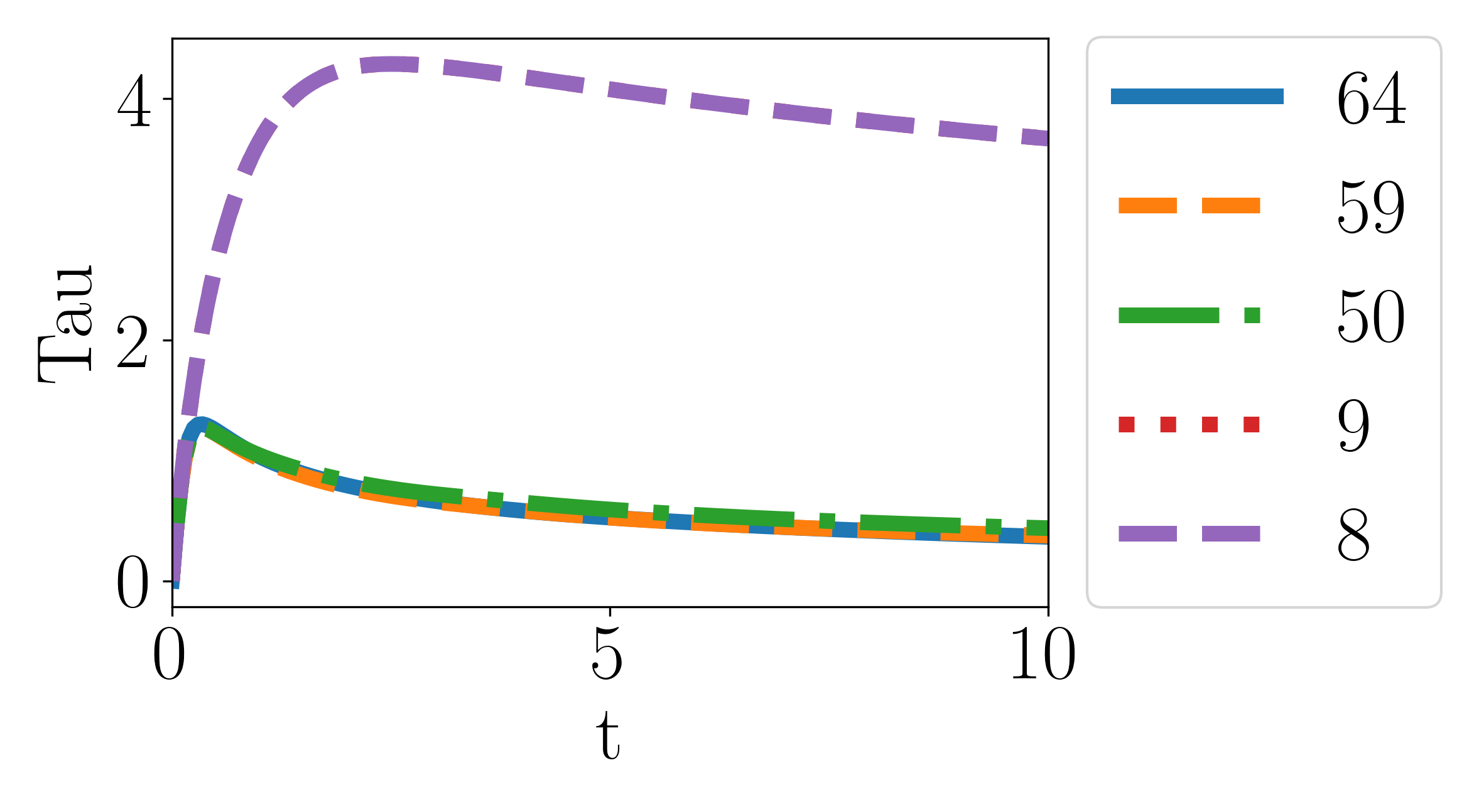
| 8 | BIOMD488 | R | [37] | Effect of A-immunization in Alzheimer’s disease | Microtubular binding protein tau (Tau) | 1/68 |
For each model, we used Algorithm 5 with to find the largest lumping tolerance such that the size of the reduced model is larger than a given bound. The bound was given as a ratio of the size of the original system. We used ratios from to using a step size of . This means that, in the case of Model 2, the initial size was 17 and so the cutoff sizes were . Notably, different ratios can lead to the same reduction. Consider Model 5. Here, the exact reduction is of the original size, so the output of Algorithm 5 is for all percentages above as they recover the exact reduction. In such cases, only one result is shown.
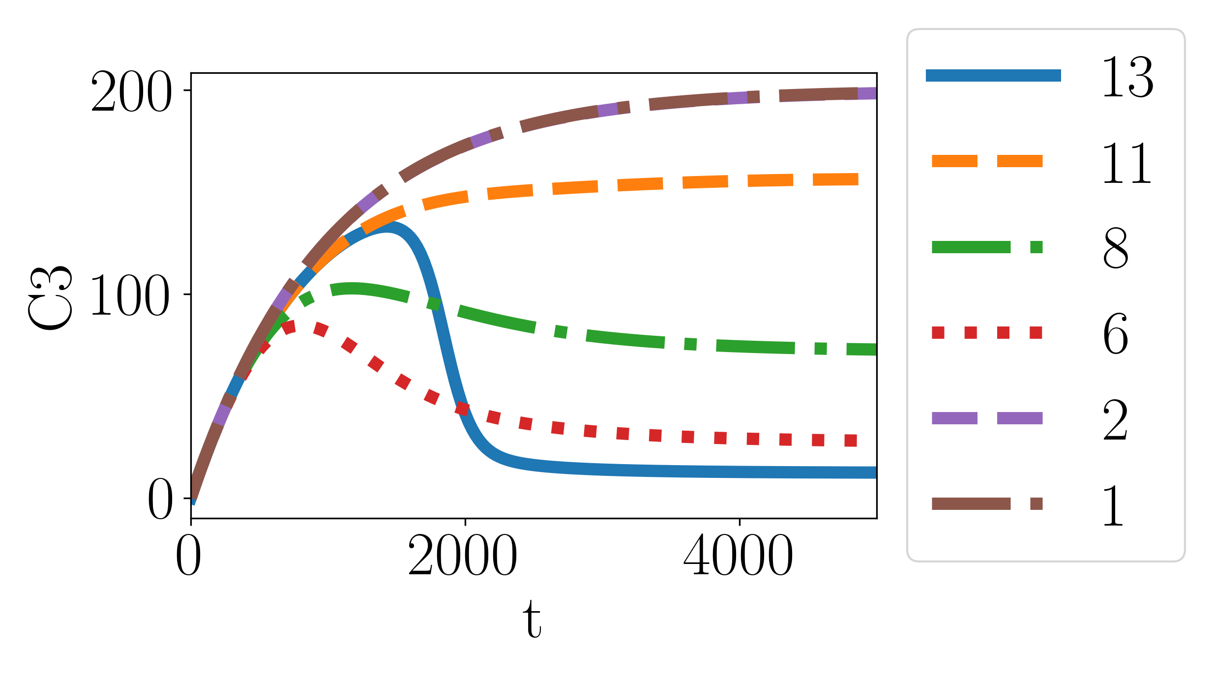
Table 2 presents the results for all models from Table 1. There is a row for each model with information constant across experiments on it, including the value for . The first column Red. shows the size of the reduced model obtained by Algorithm 4, while column Red. ratio shows the ratio between the size of the reduced model and that of the original model as a percentage. We display the absolute error and the relative error at the time horizon, respectively, in the columns and . Here, the relative error is given as the absolute error divided by the value of the observable of the exact reduction. Column shows the maximum value for within the time horizon. The obtained value of and its ratio w.r.t. are shown in the columns and , respectively. The column shows the number of iterations and the average computation time of Algorithm 5 over 5 runs. We used a 4.7 GHz Intel Core i7 computer with 32 GB of RAM to carry out all computations. For each model, we plot in Figure 8 the corresponding simulations of the observables for the considered values of . We used Scipy with RK45 and LSODA solvers to simulate polynomial and rational models respectively. Table 2 and Figure 8 show the successful use of Algorithm 5 on both polynomial and rational models.
| Red. | Red. ratio(%) | (%) | Iter. | Time (s) | ||||||
| 1) Model: BIOMD102, size: 13, type: P, exact lumping: 13, 3.52E-03 | ||||||||||
| 11 | 84.6 | 1.16E+01 | 1.44E+02 | 1.44E+02 | 4.24E-04 | 1.21E+01 | 13 | 0.284 | ||
| 8 | 61.5 | 4.86E+00 | 6.04E+01 | 6.78E+01 | 9.95E-04 | 2.83E+01 | 13 | 0.099 | ||
| 6 | 46.2 | 1.26E+00 | 1.56E+01 | 7.39E+01 | 1.73E-03 | 4.91E+01 | 13 | 0.138 | ||
| 2 | 15.4 | 1.50E+01 | 1.86E+02 | 1.86E+02 | 1.97E-03 | 5.60E+01 | 13 | 0.046 | ||
| 1 | 7.7 | 1.50E+01 | 1.86E+02 | 1.86E+02 | 3.52E-03 | 1.00E+02 | 13 | 0.052 | ||
| 2) Model: BIOMD103, size: 17, type: P, exact lumping: 17, 3.52E-03 | ||||||||||
| 14 | 82.4 | 1.02E-02 | 1.72E+00 | 1.72E+00 | 9.89E-04 | 2.81E+01 | 13 | 0.598 | ||
| 12 | 70.6 | 9.25E-01 | 1.55E+02 | 1.57E+02 | 1.60E-03 | 4.56E+01 | 13 | 0.288 | ||
| 7 | 41.2 | 8.52E-01 | 1.43E+02 | 1.44E+02 | 1.64E-03 | 4.67E+01 | 13 | 0.218 | ||
| 2 | 11.8 | 1.82E-01 | 3.06E+01 | 3.06E+01 | 2.00E-03 | 5.67E+01 | 13 | 0.070 | ||
| 3) Model: BIOMD447, size: 13, type: P, exact lumping: 13, 2.45E+01 | ||||||||||
| 11 | 84.6 | 1.33E-03 | 2.02E-05 | 2.02E-05 | 4.95E-03 | 2.02E-02 | 26 | 0.173 | ||
| 9 | 69.2 | 1.35E-02 | 2.04E-04 | 2.04E-04 | 3.41E-01 | 1.39E+00 | 26 | 0.122 | ||
| 7 | 53.8 | 8.46E-03 | 1.28E-04 | 1.29E-04 | 3.75E-01 | 1.53E+00 | 26 | 0.123 | ||
| 6 | 46.2 | 6.99E-03 | 1.06E-04 | 7.02E-04 | 1.40E+00 | 5.71E+00 | 26 | 0.105 | ||
| 3 | 23.1 | 1.22E-01 | 1.86E-03 | 7.31E-03 | 1.98E+01 | 8.10E+01 | 26 | 0.056 | ||
| 4) Model: BioNetGen_CCP, size: 87, type: P, exact lumping: 30, 2.83E+00 | ||||||||||
| 30 | 34.5 | 5.86E-06 | 6.11E-05 | 5.22E-04 | 6.74E-07 | 2.38E-05 | 23 | 1.807 | ||
| 10 | 11.5 | 3.14E-01 | 3.27E+00 | 3.27E+00 | 2.67E-01 | 9.44E+00 | 23 | 2.959 | ||
| 5) Model: NIHMS80246_S6, size: 24, type: P, exact lumping: 19, 3.13E-01 | ||||||||||
| 19 | 79.2 | 3.16E-11 | 3.16E-09 | 2.14E-04 | 5.97E-07 | 1.91E-04 | 20 | 1.370 | ||
| 17 | 70.8 | 8.09E-05 | 8.09E-03 | 4.86E+01 | 2.23E-02 | 7.13E+00 | 20 | 1.948 | ||
| 14 | 58.3 | 8.09E-05 | 8.09E-03 | 4.89E+01 | 2.34E-02 | 7.49E+00 | 20 | 1.478 | ||
| 9 | 37.5 | 1.00E+00 | 1.00E+02 | 1.00E+02 | 3.00E-02 | 9.58E+00 | 20 | 0.809 | ||
| 8 | 33.3 | 1.00E+00 | 1.00E+02 | 1.00E+02 | 1.29E-01 | 4.10E+01 | 20 | 0.586 | ||
| 1 | 4.2 | 1.00E+00 | 1.00E+02 | 1.00E+02 | 3.13E-01 | 1.00E+02 | 20 | 0.454 | ||
| 6) Model: BIOMD437, size: 39, type: R, exact lumping: 21, 7.11E+05 | ||||||||||
| 21 | 53.8 | 0.00E+00 | 0.00E+00 | 0.00E+00 | 0.00E+00 | 0.00E+00 | 1 | 0.044 | ||
| 12 | 30.8 | 1.58E-04 | 2.00E-05 | 6.66E-05 | 6.47E-07 | 9.09E-11 | 41 | 3.021 | ||
| 5 | 12.8 | 1.58E-04 | 2.00E-05 | 6.66E-05 | 1.07E+02 | 1.50E-02 | 41 | 3.645 | ||
| 4 | 10.3 | 3.31E-01 | 4.19E-02 | 4.29E-02 | 3.33E+02 | 4.69E-02 | 41 | 3.237 | ||
| 7) Model: BIOMD448, size: 27, type: R, exact lumping: 23, 1.00E+00 | ||||||||||
| 23 | 85.2 | 0.00E+00 | 0.00E+00 | 0.00E+00 | 0.00E+00 | 0.00E+00 | 1 | 0.002 | ||
| 19 | 70.4 | 7.45E-08 | 6.79E-06 | 2.90E-02 | 1.60E-02 | 1.60E+00 | 21 | 0.912 | ||
| 1 | 3.7 | 9.21E-01 | 8.39E+01 | 8.39E+01 | 1.00E+00 | 1.00E+02 | 21 | 0.291 | ||
| 8) Model: BIOMD488, size: 68, type: R, exact lumping: 64, 7.50E+10 | ||||||||||
| 59 | 86.8 | 2.88E-02 | 1.05E-02 | 2.85E-02 | 1.50E+02 | 2.00E-07 | 58 | 47.800 | ||
| 50 | 73.5 | 1.97E-01 | 7.20E-02 | 7.20E-02 | 7.50E+04 | 1.00E-04 | 58 | 46.542 | ||
| 9 | 13.2 | 9.06E+00 | 3.30E+00 | 3.61E+00 | 1.50E+06 | 2.00E-03 | 58 | 7.276 | ||
| 8 | 11.8 | 9.06E+00 | 3.30E+00 | 3.61E+00 | 6.00E+07 | 8.00E-02 | 58 | 9.505 | ||
As expected, Algorithm 5 can recover exact reductions, as seen in Models 6 and 7. Similarly, having a small cutoff size ( of the original model size or lower) results in aggressive reductions that collapse the dynamics as seen in the reduction to 8 species of Model 5 (Figure 8(e)). Taken together, these experiments display the following behaviours:
-
1.
Models that do not admit exact reduction may admit approximate reduction. Models 1, 2, and 3 were not exactly lumpable but were approximately lumped. For models 1 and 2, the reductions that incurred acceptable errors were modest, at around of the original model size. In the case of Model 3, all reductions incurred in low error, with the smallest having only species.
-
2.
Models that admit limited exact reduction, may admit smaller approximate reductions. Models 5, 7, and 8 had modest exact reductions, while they could be further reduced using approximate lumping. In this case, most of the approximate reductions have a small error. The improvement compared to the exact case goes from modest, at around of the size of the exact reduction, to as low as of the exactly reduced size (Model 5).
-
3.
Models that admit notable exact reduction, may admit even smaller approximate reductions. Models 4 and 6 had already significant exact reductions; nevertheless, they could be further reduced via approximate lumping. In this case, Model 4 shows a significant steady-state error for the approximate reduction with species. For Model 6, it was possible to find a reduction with less than of the original model size while still obtaining simulation results close to the original simulation.
As expected, for all models the error starts at and then increases with . This increment is barely noticeable when is close to for most models. While the error increases monotonically in most cases, this does not hold for all reductions. e.g., in Figures 8(a) and 8(e), the reductions with 7 and 14 species get closer to the original simulations as time increases.
Furthermore, we see that the steady-state error increases with for most models. Nonetheless, Figures 8(b) and 8(c) show that it is possible for aggressive reductions to incur lower errors. This can be explained by the influence of sampling on the representation of , as the check in Line 6 depends on the norms of each . Overall, for given models, significant reductions without large errors were obtained by Algorithm 5 with a cutoff size of of the original model size. In principle, smaller cutoff sizes may be used to find meaningful reductions; however, this requires a case-by-case analysis.
We see that rational models tend to have larger values of compared to polynomial ones (see Remark 3). This leads to more iterations of Algorithm 5. The values of that lead to low errors vary widely depending on the model. For polynomial models, most reductions happen under the threshold. Instead, for rationals the values change significantly, having reductions for lower than of . Following Remark 4, choosing a larger value for in Model 8 would have led to fewer iterations and faster times at the cost of potentially missing some low-error reductions as these happened for low values of . Finally, we note that assumptions of Theorem 3.1 were satisfied by the experiments since the obtained approximate lumpings led to positive for all positive vectors , while the denominators of rational vanished only for negative values of .
4.2 Scalability analysis
We evaluate the scalability of our approach using a parametric model of multisite protein phosphorylation which can be made combinatorially larger by increasing its number of binding sites [41]. This mechanism is key in the study of cellular processes [20]. The model describes the phosphorylation and dephosphorylation of a substrate with different binding sites, each capable of being in 4 different states [44]. The resulting model requires variables to track the evolution of all protein configurations as well as the kinase and phosphatase concentrations.
The exact constrained lumping of this model was studied in [35]. We choose the concentration of free kinase as the observable of interest. For our setup, we added random noise to each reaction, taken from to of the parameter value appearing in each reaction (the same parameter could have different values for different reactions). This ensured that the perturbed model was not exactly reducible. Next, we ran Algorithm 5 with a maximum reduction size and for models with 2 to 5 binding sites. To compute the error, the time horizon was set to , and the initial conditions were taken from the original paper. All simulations were computed using the LSODA stiff solver.
| Sites | Size | Red. Size | Iter. | Time (min) | Original (s) | Red. (s) | (%) | ||
|---|---|---|---|---|---|---|---|---|---|
| 2 | 24 | 5 | 8 | 0.003 | 0.116 | 0.022 | 0.018 | 2.60 | 0.274 |
| 3 | 72 | 4 | 8 | 0.214 | 0.186 | 0.020 | 0.004 | 1.00 | 0.236 |
| 4 | 264 | 4 | 8 | 8.024 | 1.429 | 0.032 | 0.001 | 0.30 | 0.208 |
| 5 | 1032 | 4 | 8 | 371.683 | 13.303 | 0.025 | 0.001 | 0.60 | 0.199 |
Table 3 presents the results for multisite phosphorylation models. Column Sites displays the number of binding sites in the model. The size of the original model and that of the reduced model are shown in the columns Size and Red. Size, respectively. The number of iterations and the total computation time of Algorithm 5 are displayed in the columns Iter. and Time, respectively. The columns Original and Red. contain the time used to compute the simulation using the non-reduced model and the reduced model, respectively. The absolute and relative error at steady-state are shown in the columns and . While the maximum absolute error is shown in .
As seen in Table 3, our approach can find a reduction with only 4 species for a model without exact reductions. These reductions have low errors (less than for all models). This is a promising result for the study of more robust reductions. The runtime depends on the size of the model. Larger models take considerably longer as there is a combinatorial increment in the number of monomials needed to represent the Jacobian. This, in turn, gets amplified by the number of iterations necessary to find a lumping with the given size restriction, which depends on the tolerance for Algorithm 5.
5 Conclusion
We have proposed approximate constrained lumping, a relaxation of the exact reduction technique constrained lumping. This allows for more aggressive reductions at the cost of introducing, in a controlled way, errors in the dynamics of the reduced model. The technique can be applied to dynamical systems with polynomial or rational derivatives, common in computational biology. For a given dynamical system, our algorithm utilizes a numerical tolerance to efficiently compute a reduced system that preserves the evolution of a linear combination of specific variables of interest up to a bounded error. We proved that the error bound is proportional to the numerical threshold. Additionally, we introduced a heuristic to obtain appropriate numerical tolerances based on the model size. We demonstrated effectiveness and scalability by obtaining low-error reductions for a collection of published biological models. Future work will explore robust reductions by considering models with uncertain kinetic parameters.
References
- [1] A. Antoulas. Approximation of Large-Scale Dynamical Systems. Advances in Design and Control. SIAM, 2005.
- [2] Mochamad Apri, Maarten de Gee, and Jaap Molenaar. Complexity reduction preserving dynamical behavior of biochemical networks. Journal of Theoretical Biology, 304(0):16–26, 2012.
- [3] Ann Babtie and Michael Stumpf. How to deal with parameters for whole-cell modelling. J. of The Royal Society Interface, 14(133):20170237, 2017.
- [4] Giorgio Bacci, Giovanni Bacci, Kim G. Larsen, and Radu Mardare. On-the-fly exact computation of bisimilarity distances. In Nir Piterman and Scott A. Smolka, editors, TACAS, volume 7795 of Lecture Notes in Computer Science, pages 1–15, 2013.
- [5] Jiri Barnat, Nikola Benes, Lubos Brim, Martin Demko, Matej Hajnal, Samuel Pastva, and David Safránek. Detecting attractors in biological models with uncertain parameters. In Jérôme Feret and Heinz Koeppl, editors, CMSB, volume 10545 of Lecture Notes in Computer Science, pages 40–56. Springer, 2017.
- [6] M. L. Blinov, J. R. Faeder, B. Goldstein, and W. S. Hlavacek. BioNetGen: software for rule-based modeling of signal transduction based on the interactions of molecular domains. Bioinformatics, 20(17):3289–3291, 2004.
- [7] Nikolay M. Borisov, Alexander S. Chistopolsky, James R. Faeder, and Boris N. Kholodenko. Domain-Oriented Reduction of Rule-Based Network Models. IET systems biology, 2(5):342–351, September 2008.
- [8] Cecilia Brännmark, Elin Nyman, Siri Fagerholm, Linnéa Bergenholm, Eva-Maria Ekstrand, Gunnar Cedersund, and Peter Strålfors. Insulin signaling in type 2 diabetes: experimental and modeling analyses reveal mechanisms of insulin resistance in human adipocytes. The Journal of Biological Chemistry, 288(14):9867–9880, April 2013.
- [9] Francesca Cairoli, Ginevra Carbone, and Luca Bortolussi. Abstraction of markov population dynamics via generative adversarial nets. In Eugenio Cinquemani and Loïc Paulevé, editors, CMSB, volume 12881, pages 19–35, 2021.
- [10] Luca Cardelli. From processes to odes by chemistry. In Giorgio Ausiello, Juhani Karhumäki, Giancarlo Mauri, and Luke Ong, editors, Fifth Ifip International Conference On Theoretical Computer Science – Tcs 2008, 2008.
- [11] Luca Cardelli, Isabel Cristina Pérez-Verona, Mirco Tribastone, Max Tschaikowski, Andrea Vandin, and Tabea Waizmann. Exact maximal reduction of stochastic reaction networks by species lumping. Bioinform., 37(15):2175–2182, 2021.
- [12] Luca Cardelli, Mirco Tribastone, Max Tschaikowski, and Andrea Vandin. Forward and backward bisimulations for chemical reaction networks. In CONCUR, pages 226–239, 2015.
- [13] Luca Cardelli, Mirco Tribastone, Max Tschaikowski, and Andrea Vandin. Comparing chemical reaction networks: A categorical and algorithmic perspective. In Martin Grohe, Eric Koskinen, and Natarajan Shankar, editors, Proceedings of the 31st Annual ACM/IEEE Symposium on Logic in Computer Science, LICS ’16, New York, NY, USA, July 5-8, 2016, pages 485–494. ACM, 2016.
- [14] Luca Cardelli, Mirco Tribastone, Max Tschaikowski, and Andrea Vandin. ERODE: A Tool for the Evaluation and Reduction of Ordinary Differential Equations. In Axel Legay and Tiziana Margaria, editors, Tools and Algorithms for the Construction and Analysis of Systems, Lecture Notes in Computer Science, pages 310–328, Berlin, Heidelberg, 2017. Springer.
- [15] Luca Cardelli, Mirco Tribastone, Max Tschaikowski, and Andrea Vandin. Maximal aggregation of polynomial dynamical systems. PNAS, 114(38):10029–10034, 2017.
- [16] Luca Cardelli, Mirco Tribastone, Max Tschaikowski, and Andrea Vandin. Guaranteed error bounds on approximate model abstractions through reachability analysis. In Annabelle McIver and András Horváth, editors, Quantitative Evaluation of Systems - 15th International Conference, QEST 2018, Beijing, China, September 4-7, 2018, Proceedings, volume 11024 of Lecture Notes in Computer Science, pages 104–121. Springer, 2018.
- [17] Luca Cardelli, Mirco Tribastone, Max Tschaikowski, and Andrea Vandin. Symbolic computation of differential equivalences. Theoretical Computer Science, 777:132–154, 2019.
- [18] Przemyslaw Daca, Thomas A. Henzinger, Jan Kretínský, and Tatjana Petrov. Linear distances between markov chains. In Josée Desharnais and Radha Jagadeesan, editors, CONCUR, volume 59 of LIPIcs, pages 20:1–20:15, 2016.
- [19] Jérôme Feret, Vincent Danos, Jean Krivine, Russ Harmer, and Walter Fontana. Internal coarse-graining of molecular systems. PNAS, 106(16):6453–6458, 2009.
- [20] Jeremy Gunawardena. Multisite protein phosphorylation makes a good threshold but can be a poor switch. PNAS, 102(41):14617–14622, 2005.
- [21] Martin Helfrich, Milan Ceska, Jan Kretínský, and Stefan Marticek. Abstraction-based segmental simulation of chemical reaction networks. In Ion Petre and Andrei Paun, editors, CMSB, volume 13447, pages 41–60, 2022.
- [22] Jane Hillston, Mirco Tribastone, and Stephen Gilmore. Stochastic Process Algebras: From Individuals to Populations. The Computer Journal, 55(7):866–881, 2011.
- [23] Giulio Iacobelli and Mirco Tribastone. Lumpability of fluid models with heterogeneous agent types. In 2013 43rd Annual IEEE/IFIP International Conference on Dependable Systems and Networks (DSN), pages 1–11, June 2013. ISSN: 2158-3927.
- [24] Antonio Jiménez-Pastor, Joshua Paul Jacob, and Gleb Pogudin. Exact linear reduction for rational dynamical systems. In Computational Methods in Systems Biology, pages 198–216. Springer International Publishing, 2022.
- [25] Kim G. Larsen and Arne Skou. Bisimulation through probabilistic testing. Inf. Comput., 94(1):1–28, 1991.
- [26] Stefan Legewie, Nils Blüthgen, and Hanspeter Herzel. Mathematical modeling identifies inhibitors of apoptosis as mediators of positive feedback and bistability. PLoS computational biology, 2(9):e120, September 2006.
- [27] Alexander Leguizamon-Robayo, Antonio Jiménez-Pastor, Micro Tribastone, Max Tschaikowski, and Andrea Vandin. Approximate Constrained Lumping of Polynomial Differential Equations. In Jun Pang and Joachim Niehren, editors, Computational Methods in Systems Biology, Lecture Notes in Computer Science, pages 106–123, Cham, 2023. Springer Nature Switzerland.
- [28] Chen Li, Marco Donizelli, Nicolas Rodriguez, Harish Dharuri, Lukas Endler, Vijayalakshmi Chelliah, Lu Li, Enuo He, Arnaud Henry, Melanie Stefan, Jacky Snoep, Michael Hucka, Nicolas Le Novère, and Camille Laibe. BioModels Database: An enhanced, curated and annotated resource for published quantitative kinetic models. BMC Systems Biology, 4:92, 2010.
- [29] Genyuan Li and Herschel Rabitz. A general analysis of exact lumping in chemical kinetics. Chemical Engineering Science, 44(6):1413–1430, 1989.
- [30] Genyuan Li and Herschel Rabitz. A general analysis of approximate lumping in chemical kinetics. Chemical Engineering Science, 45(4):977–1002, 1990.
- [31] Genyuan Li and Herschel Rabitz. New approaches to determination of constrained lumping schemes for a reaction system in the whole composition space. Chemical Engineering Science, 46(1):95–111, 1991.
- [32] Christoph Lüders, Thomas Sturm, and Ovidiu Radulescu. ODEbase: A repository of ODE systems for systems biology. Bioinformatics Advances, 2(1), April 2022. vbac027.
- [33] Fangping Mu, Robert F. Williams, Clifford J. Unkefer, Pat J. Unkefer, James R. Faeder, and William S. Hlavacek. Carbon-fate maps for metabolic reactions. Bioinformatics (Oxford, England), 23(23):3193–3199, December 2007.
- [34] M. Okino and M. Mavrovouniotis. Simplification of mathematical models of chemical reaction systems. Chemical Reviews, 2(98):391–408, 1998.
- [35] Alexey Ovchinnikov, Isabel Pérez Verona, Gleb Pogudin, and Mirco Tribastone. CLUE: exact maximal reduction of kinetic models by constrained lumping of differential equations. Bioinformatics, 37(12):1732–1738, June 2021.
- [36] Isabel Cristina Pérez-Verona, Mirco Tribastone, and Andrea Vandin. A large-scale assessment of exact model reduction in the BioModels repository. In Computational Methods in Systems Biology, pages 248–265. Springer International Publishing, 2019.
- [37] Carole J. Proctor, Delphine Boche, Douglas A. Gray, and James A. R. Nicoll. Investigating interventions in Alzheimer’s disease with computer simulation models. PloS One, 8(9):e73631, 2013.
- [38] Ovidiu Radulescu, Alexander N Gorban, Andrei Zinovyev, and Vincent Noel. Reduction of dynamical biochemical reactions networks in computational biology. Frontiers in genetics, 3:131, 2012.
- [39] Denis Repin and Tatjana Petrov. Automated deep abstractions for stochastic chemical reaction networks. Inf. Comput., 281:104788, 2021.
- [40] Walter Rudin. Principles of Mathematical Analysis. McGraw-Hill, 1976.
- [41] Carlos Salazar and Thomas Höfer. Multisite protein phosphorylation — from molecular mechanisms to kinetic models. FEBS Journal, 276(12):3177–3198, 2009.
- [42] Henning Schmidt, Mads Madsen, Sune Danø, and Gunnar Cedersund. Complexity reduction of biochemical rate expressions. Bioinformatics, 24(6):848–854, 2008.
- [43] L.A. Segel and M. Slemrod. The quasi-steady-state assumption: A case study in perturbation. SIAM Review, 31(3):446–477, 1989.
- [44] Michael Sneddon, James Faeder, and Thierry Emonet. Efficient modeling, simulation and coarse-graining of biological complexity with NFsim. Nature methods, 8(2):177, 2011.
- [45] Thomas Snowden, Piet van der Graaf, and Marcus Tindall. Methods of model reduction for large-scale biological systems: A survey of current methods and trends. Bulletin of Mathematical Biology, 79(7):1449–1486, 2017.
- [46] Mikael Sunnaker, Gunnar Cedersund, and Mats Jirstrand. A method for zooming of nonlinear models of biochemical systems. BMC Systems Biology, 5(1):140, 2011.
- [47] Stefano Tognazzi, Mirco Tribastone, Max Tschaikowski, and Andrea Vandin. Egac: A genetic algorithm to compare chemical reaction networks. In GECCO, GECCO ’17, pages 833–840, 2017.
- [48] Alison S. Tomlin, Genyuan Li, Herschel Rabitz, and János Tóth. The Effect of Lumping and Expanding on Kinetic Differential Equations. SIAM Journal on Applied Mathematics, 57(6):1531–1556, December 1997. Publisher: Society for Industrial and Applied Mathematics.
- [49] Mirco Tribastone. Behavioral relations in a process algebra for variants. In Stefania Gnesi, Alessandro Fantechi, Patrick Heymans, Julia Rubin, Krzysztof Czarnecki, and Deepak Dhungana, editors, SPLC, pages 82–91. ACM, 2014.
- [50] Matej Troják, David Safránek, Samuel Pastva, and Lubos Brim. Rule-based modelling of biological systems using regulated rewriting. Biosyst., 225:104843, 2023.
- [51] Max Tschaikowski and Mirco Tribastone. Exact fluid lumpability in markovian process algebra. Theoretical Computer Science, 538:140–166, 2014.
- [52] Max Tschaikowski and Mirco Tribastone. Approximate reduction of heterogeneous nonlinear models with differential hulls. IEEE TAC, 2016.
- [53] Max Tschaikowski and Mirco Tribastone. Spatial fluid limits for stochastic mobile networks. Perform. Evaluation, 109:52–76, 2017.
- [54] Yu-Yao Tseng, Suzanne M. Hunt, Christian Heintzen, Susan K. Crosthwaite, and Jean-Marc Schwartz. Comprehensive modelling of the Neurospora circadian clock and its temperature compensation. PLoS computational biology, 8(3):e1002437, 2012.
- [55] Ravishankar Vallabhajosyula, Vijay Chickarmane, and Herbert Sauro. Conservation analysis of large biochemical networks. Bioinformatics, 22(3):346–353, 2005.
- [56] Lakshmi Venkatraman, Ser-Mien Chia, Balakrishnan Chakrapani Narmada, Jacob K. White, Sourav S. Bhowmick, C. Forbes Dewey, Peter T. So, Lisa Tucker-Kellogg, and Hanry Yu. Plasmin triggers a switch-like decrease in thrombospondin-dependent activation of TGF-1. Biophysical Journal, 103(5):1060–1068, September 2012.
- [57] Eberhard O. Voit. Biochemical systems theory: A review. ISRN Biomathematics, 2013:53, 2013.
- [58] Max Whitby, Luca Cardelli, Marta Kwiatkowska, Luca Laurenti, Mirco Tribastone, and Max Tschaikowski. PID control of biochemical reaction networks. IEEE Trans. Autom. Control., 67(2):1023–1030, 2022.
- [59] Martin Wirsing, Matthias Hölzl, Lucia Acciai, Federico Banti, Allan Clark, Alessandro Fantechi, Stephen Gilmore, Stefania Gnesi, László Gönczy, Nora Koch, Alessandro Lapadula, Philip Mayer, Franco Mazzanti, Rosario Pugliese, Andreas Schroeder, Francesco Tiezzi, Mirco Tribastone, and Dániel Varró. Sensoria patterns: Augmenting service engineering with formal analysis, transformation and dynamicity. In Tiziana Margaria and Bernhard Steffen, editors, Leveraging Applications of Formal Methods, Verification and Validation, pages 170–190, 2008.
Appendix: Proofs
Proposition 1
Let a system of ODEs such that is analytic on a compact set . Given a lumping , such that for all , the norm of the error is bounded as follows
Proof
Note that for any initial condition , we can compute
To bound the first term, recall that is analytic on . Therefore is locally Lipschitz in . Then there is a constant such that
for all and all .
Using the fact that is an lumping, we get that
for all and all . The result follows by setting .
Lemma 2
[23, Lemma 2]. Let be a continuous scalar function on which has a right derivative such that
for all , where and re constants and . Then
for all .
Proof (Theorem 3.1)
Proof (Theorem 3.2)
We first prove the polynomial complexity of Algorithm 4. To this aim, we assume a naive implementation of the matrix operations. We begin by analyzing the complexity of the operations performed in the main loop (Line 4) of Algorithm 4. To find the complexity of computing , recall that is an matrix. This means that computing can be done in , while can be computed in . Hence, can be computed in . Since and are of dimensions , computing has complexity . Instead, computing has complexity . Overall, we have that the complexity of the operations inside the main loop (Line 4) of Algorithm 4 is . As this loop is computed times, we have that the total complexity of Algorithm 4 is . The result follows from the fact that Algorithm 1 can be implemented with a complexity of , where is the arithmetic cost of computing an entry of .
Theorem 0..1
Proposition 2
Proof
Fix , by hypothesis . Let .
We claim that
| (10) |
where is a constant, and is the projection onto .
Note that , where is the Jacobian of and is the inclusion given by .
We compute
| (11) |
where is the norm restricted to .
Following Equation (11), we have to estimate
| (12) |
To this aim, we will first estimate each entry of the vector . Denote by , the vector of zeroes with one in the th entry, and denote by the th row of . Let . Given that , we have that
Using the fact that , we have
Using the triangle inequality, and the Cauchy-Schwartz inequality we have that
| (13) |
where is the tolerance used in the computation of Algorithm 4.
Since is analytic in , we have that its derivative is bounded in . Therefore each is bounded in and so, by the extreme value theorem, there exists a constant such that
| (14) |
Combining Equation (14) with the previous reasoning we have that
| (15) |
Using Equations (11) and (15), we get that
| (16) |
As is a linear map, the set is open and convex. Therefore, we can use Equation (16) and Theorem 0..1 to show that
| (17) |
Notice that is the projection of onto the rowspace of . It follows that , and so . Moreover since , it follows that . So we can set and in Equation (17) to get that
where there last result follows from the definition of and the fact that , as we wanted to prove.
Proposition 3
Let be an analytic function on a compact set . Assume we can write in the form given by Equation 3, where and are -linearly independent and analytic on . Consider such that is a basis of the vector space . Given a matrix if there is an such that for all and all rows of of
then there exists a constant such that for all and all rows of we have
Proof
It is clear that the matrices generate the space and they belong to it. At the same time, we have by assumption that is a basis of . Hence:
Multiplying by to the left, we obtain: .
Therefore, all rows of are linear combinations of rows of the matrices . Let us denote by and the -th row of and of , resp. Then we have: , which means that:
Thus, the statement is true by taking .
Lemma 3
Proof
Recall, the extended Algorithm 4 checks that for all rows of and all , where . By using Proposition 3, we get that there is a constant such that for all , where, by hypothesis, we can write with and being -linearly independent and analytic on . We follow the reasoning of the proof of Proposition 2, up to Equation Proof. There by the fact that each is bounded, we have that
where . The result follows by continuing the aforementioned reasoning.
Proof (Theorem 3.3)
As is analytic in , we can use Lemma 3 for each and each solution with initial conditions in to get
| (18) |
for all .
Proof (Lemma 1)
Consider a matrix of observables of rank with th row denoted by and a decomposition of the Jacobian . Let be given by Equation 8. It follows that for all and . Using (or any as input for Algorithm 4 implies that the condition in Line 6 will be false. Thus, exiting the loop and returning a matrix whose rows are orthonormal rows spanning .
To show that is the lowest upper bound on , assume is such that Algorithm 4 outputs orthonormal rows spanning . This implies that . By the definition of , it follows that , as we wanted to prove.