Path Tracking Hybrid A* For Autonomous Agricultural Vehicles

Abstract

We propose a path-tracking Hybrid A* planner and a coupled hierarchical Model Predictive Control (MPC) controller in scenarios involving the path smoothing of agricultural vehicles. For agricultural vehicles following reference paths on farmlands, especially during cross-furrow operations, a minimum deviation from the reference path is desired, in addition to the curvature constraints and body scale collision avoidance. Our contribution is threefold. (1) We propose the path-tracking Hybrid A*, which satisfies nonholonomic constraints and vehicle size collision avoidance, and devise new cost and heuristic functions to minimize the deviation degree. The path-tracking Hybrid A* can not only function in offline smoothing but also the real-time adjustment when confronted with unexpected obstacles. (2) We propose the hierarchical MPC to safely track the smoothed trajectory, using the initial solution solved by linearized MPC and nonlinear local adjustments around the initial solution. (3) We carry out extensive simulations with baseline comparisons based on real-world farm datasets to evaluate the performance of our algorithm.

I Introduction

With the rapid advancements in robotics technologies in recent years, autonomous mobile robots have been extensively utilized across various domains, including industry, service, and agriculture[1]. Among all the techniques, smooth path planning is an indispensable component of any mobile robot. In the literature, smooth path planning studies are carried out in two steps, referred to as “front end” and “back end”. The “front end” usually implements the sampling or search-based path planning algorithms, such as the A*[2], Hybrid A*[3], rapidly-exploring random tree (RRT)[4], probabilistic roadmap (PRM)[5] and artificial potential field[6], to generate a raw path from the start point to the end point while avoiding collision with obstacles in the environment. However, many path-planning algorithms, such as A*, RRT, and PRM, take no account of the robot’s kinematic model, resulting in generating raw paths with sharp turns, which are difficult for the robot to track. The “back end”, i.e., path smoothing, addresses this issue by modifying the raw path considering robot kinematic constraints, and obstacle avoidance, to generate spatial-temporal trajectories of the robot, which is easier for the robot to follow. However, these methods pay their most attention to geometric continuity and curvature limits, which are generic but not the most crucial elements in certain scenarios, such as the agricultural use introduced here. The cultivation between furrows requires the agricultural vehicle to cross the furrows. The reference trajectory for crossing the furrows is typically marked manually or extracted by “front-end” algorithms. During the cross-furrow operation, the vehicle should adhere closely to the reference paths to trample less on the farmlands and prevent crop damage, calling for the need to minimize the deviation degree of the smoothed trajectories. This has inspired us to propose a new methodology of path smoothing: using the search-based algorithm which contains a heuristic function and conforms to the nonholonomic constraints to directly solve the path smoothing problem. Therefore, a path-tracking Hybrid A* algorithm may be the most appropriate in this context.

Path planning is always a key focus for agricultural robots [7] with unique challenges, such as terrain irregularity, multi-task handling, field coverage, etc. Santos et al.[8] limit the roll, pitch, and yaw angles considering the center of mass of the robot to tackle the irregularity of farmland terrain, and Mai et al.[9] find a solution for multi-point monitoring process in potato cultivation. Besides, field coverage[10, 11, 12] and energy optimization[13] are also discussed. However, research on avoiding crop damage is relatively rare, which inspires us to design algorithms that minimize the deviation from the reference trajectory.

In recent years, there have been many works [14, 15, 16, 17, 18] focusing on Hybrid A* and its application. Hybrid A* is a search-based path planning algorithm that combines the discrete grid search of A* with continuous space optimization, enabling the generation of feasible and smooth paths that account for vehicle kinematics. Recent works apply the Hybrid A* algorithm in conjunction with other methods: with the Visibility Diagram planning[14], with the safe travel corridor model[15], with the time-elastic-band[16], with hierarchical clustering[17], and with multistage dynamic optimization[18], to enhance computational speed and optimize local trajectories. However, to the best of our knowledge, all these works utilize the Hybrid A* path planner as the “front end” in navigation or parking scenarios, while no previous work has applied it in path smoothing.

The state-of-the-art path smoothing methods include the following types[19]: interpolation, special curves, and optimization-based path smoothing. First, interpolation methods involve employing parameterized curves, such as the polynomial curve, the Bézier curve, or the B-spline curve, to fit the raw path generated by the front end. The polynomial interpolation is a traditional method and is limited by Runge’s phenomenon[20]. The Bézier curve interpolation is researched thoroughly due to its capability to satisfy $C^{2}$ continuity and curvature constraints[21], or endpoints and via points constraints[22]. Low-order Bézier curves such as quadratic Bézier curves are used to prune the control points[23] or even build curvature-continuous smooth path[24]. In terms of B-spline, real-time $C^{2}$ continuous B-splines with curvature limits[25] or with collision avoidance[26] are widely used in the path smoothing literature, and recent B-spline path smoothing method [27] further eliminate jerky and unnecessary motions by introducing the Douglas-Peucker algorithm into the path pruning technique.

Second, path smoothing based on special curves mainly includes clothoid and Dubin’s curve, which are difficult to parameterize compared to the interpolation curves. The clothoids, also known as Euler spirals[28], are parameterized by their arc length and show a linear variation in curvature along their length. Lambert et al.[29] exhibit that clothoid-based path smoothing can be used to automatically plan diversions that can be traversed at high speed by automated vehicles, and Lin et al.[30] use clothoid to generate smooth emergency-stopping paths. Dubin’s curve[31] and Reeds-Shepp curve[32], which consist of line segments and circular arcs, are used to find the shortest paths between two configurations conforming to vehicle kinematic constraints[33].

The last category, the optimization-based method, is mostly seen combined with the methods mentioned above in the literature, which can simultaneously consider multiple optimization objectives, such as obstacle avoidance, rollover constraints, speed, acceleration, jerk, etc, to find a balanced solution. The current mainstream optimization methods can be adapted to the curves mentioned above, such as the particle swarm optimization (PSO) to the Bézier curve[34, 35, 36], and the ant colony optimization (ACO) to the B-spline curve[37, 38].

However, the abovementioned methods have two major drawbacks when applied to our circumstances. Most importantly, most works pay no attention to minimize the deviation degree between the smoothed trajectory and the reference path, which is a key requirement in our agricultural scenario. In addition, most works generate trajectories that avoid collision based on the point-mass model, neglecting the vehicle’s size, while in our context the distance from the reference trajectory to the boundary is at the same scale as the vehicle size, which makes whole-body collision avoidance necessary.

To bridge the gaps, we propose a novel cross-furrow path planning method for agricultural vehicles. The main contribution of this paper is threefold: First, we propose the path-tracking Hybrid A*, which satisfies nonholonomic constraints and vehicle size collision avoidance, bring it into the field of path smoothing, and devise new cost and heuristic functions to minimize the deviation degree. Note that the path-tracking Hybrid A* can be used in not only the offline smoothing of the reference paths but also the real-time adjustments of the smoothed trajectories when confronted with obstacles unknown beforehand. Second, we adopt a hierarchical MPC to track the smoothed trajectory, with the initial solution solved by linearized MPC and nonlinear local adjustments around the initial solution. Third, we carry out extensive simulations with baseline comparisons based on real-world farm datasets to evaluate the performance of our algorithm.

The remainder of this paper is organized as follows: Section II mathematically defines the model of farm and agricultural vehicles. Section III-A reviews the basic principles of Hybrid A*. Section III-B and section III-C propose the path-tracking Hybrid A* algorithm, most importantly the deviation-aware cost and heuristic functions and the pruning techniques. Section III-D shows the adjusted path-tracking Hybrid A* method of obstacle avoidance, and section III-E shows the hierarchical MPC tracking technique. Section IV exhibits the simulation results tested on static real-world cross-furrow reference paths, and then exhibits the test results of real-time obstacle avoidance performance of the planning-control system.

II Problem Formulation

We are considering the cross-furrow path planning problem for agricultural vehicles when operating on farmland. The agricultural vehicles are tasked with planning their motion trajectory, closely following the reference path between different furrows, which is manually annotated or generated by the front-end algorithm, while ensuring avoidance constraints with the edges of the field.

II-A Farm Modeling

We formulate the farm as a two-dimensional polygon-shaped region $P\in\mathbb{R}^{2}$, which is defined by the polygon vertices $\mathcal{V}=\{v_{1},v_{2},\dots,v_{n}\}$ and edges $\mathcal{E}=\{e_{1},e_{2},\dots,e_{n}\}$.

Within the farm $P$, the movement of agricultural vehicles should align with the cross-furrow reference paths. Each reference path $R\subset P$ is a polyline consisting of a sequence of line segments $\mathcal{L}=\{l_{1},l_{2},\dots,l_{m}\}$, where each line segment $l_{j}\subset P$ connects waypoints $p_{j}$ and $p_{j+1}$.

II-B Motion Model of Agricultural Vehicle

We consider an agricultural vehicle formulated as a Wheeled Mobile Robot (WMR). Specifically, the kinematics of the WMR is formulated as the following bicycle model:

$$\begin{cases}\dot{x}=v\cos\theta,\\ \dot{y}=v\sin\theta,\\ \dot{\theta}=v\frac{tan\delta}{L},\\ \dot{v}=a,\end{cases}$$ (1)

where $L$ denotes the wheelbase, and the state vector $\boldsymbol{x}=[x,y,\theta,v]^{T}$ indicates the configuration of the WMR, including the position $[x,y]^{T}\in\mathbb{R}^{2}$, orientation $\theta\in\mathbb{R}$, and linear velocity of the rear wheel axis center, $C$. The control input $\boldsymbol{u}=[\delta,a]^{T}$ comprises the wheel steering angle $\delta$ (with a maximum value $\delta_{m}$) and the linear acceleration $a$. Applying Euler’s approximation to eq. 1, we obtain the discrete-time version of the kinematic model:

$$\begin{cases}x_{k+1}=x_{k}+v_{k}\cos\theta_{k}\Delta t,\\ y_{k+1}=y_{k}+v_{k}\sin\theta_{k}\Delta t,\\ \theta_{k+1}=\theta_{k}+v_{k}\frac{tan\delta_{k}}{L}\Delta t,\\ v_{k+1}=v_{k}+a_{k}\Delta t,\end{cases}$$ (2)

where $\Delta t$ is the sampling interval. For notational simplicity, we reformulate eq. 2 as the following compact representation:

$$\boldsymbol{x}_{k+1}=f_{d}(\boldsymbol{x}_{k},\boldsymbol{u}_{k}).$$ (3)

II-C Path Smoothing Problem Description

Our objective is to find a smoothed trajectory $\tau(t):\mathbb{R}\to\mathbb{R}^{2}$ for the agricultural vehicle, which is confined in $\mathcal{V}$ and conforms to the kinematics (eq. 1), and has a minimum deviation degree from $\mathcal{R}$. The key points of the smoothed trajectory are defined as $x_{n}=\tau(n\Delta t),n=0,1,2,\dots$, where $\Delta t$ is the sampling interval.

III Path Tracking Hybrid A* Algorithm

Our approach is divided into two stages. Initially, by modifying the Hybrid A* algorithm, we devise novel heuristic functions to generate smoothed trajectories that are closely aligned with the reference paths, which is shown in algorithm 1. Besides, section III-D shows the adjusted path-tracking Hybrid A* method of real-time obstacle avoidance. Second, section III-E incorporates the hierarchical MPC algorithm, which robustly tracks the smoothed trajectory.

III-A Basic Principle of Hybrid A*

The Hybrid A* algorithm [3] is an extension of the traditional A* path-search algorithm, which is designed to handle continuous spaces and nonholonomic constraints (constraints on the motion of vehicles that cannot be captured by purely holonomic constraints) for path planning. Here we briefly review the basic principles of Hybrid A*.

Search Space. Hybrid A* generates paths through a blend of discrete and continuous space exploration. Specifically, Hybrid A* discretizes the continuous search space into a grid, while allowing movements based on the kinematic model of the vehicle instead of being limited to grid alignments as traditional A* does. This approach helps Hybrid A* to closely represent vehicle dynamics and constraints, such as turning radii, in the process of finding the optimal path. The search process is based on nodes, each containing the information of current state $[x,y,\theta]^{T}$, the previous node, and the total cost $f$. Note that each grid can only contain one forward and backward node respectively.

Cost and Heuristic Functions. Hybrid A* employs both a cost function $g$ and a heuristic function $h$ to optimize pathfinding. The cost $g$ accounts for the accumulated distance from the start, adding penalties for vehicular maneuvers such as steering changes or reversing. The heuristic function $h$, which is the max of the non-holonomic-without-obstacles cost and 2D Euclidean distance [3], determines the direction of the search, preventing aimless exploration and thus improving search speed. In general, the total cost function to be minimized can be stated as

$$f=g+h.$$ (4)

• 

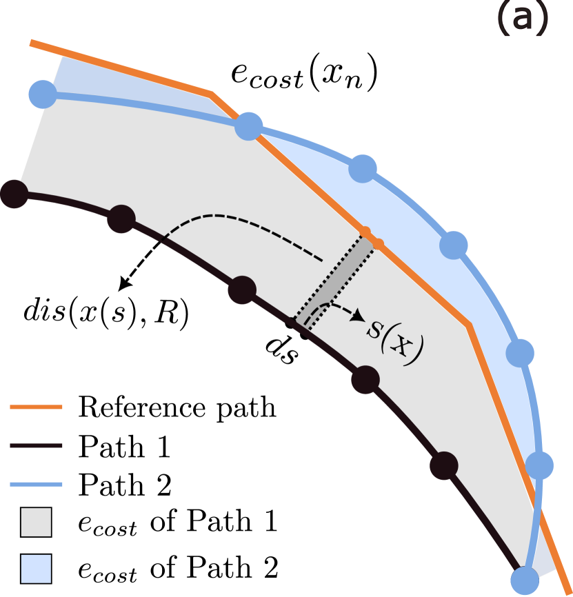
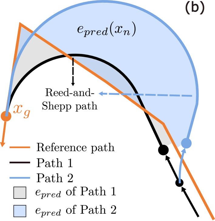
Figure 1: Illustration for the cost (a) and heuristic (b) for path smoothing. (a): the shaded area illustrates the deviation cost calculated by eq. 6, and the $e_{cost}$ of Path 1 is larger than that of Path 2. (b): Two nodes are extended from their parent node, and each is connected to the goal point with a Reed-and-Shepp path. Note that due to the divergent orientation of Path 2, the $e_{pred}$ of Path 2 is significantly larger than that of Path 1. Therefore, the heuristic eq. 9 is useful in burning the wrong heading nodes.

III-B Deviation-Aware Cost and Heuristic for Path Smoothing

One of the most significant contributions of our work is the design of deviation-aware cost and heuristic functions to adapt the Hybrid A* for path smoothing. As stated in section III-A, in traditional Hybrid A*, the cost and heuristic functions were mainly aimed at minimizing the length of the planned trajectory. However, in our problem context, it is imperative to also take into account the degree of deviation from a reference path, thus guiding the generated trajectory to more closely align with the reference path. First, we defined the distance from a node to the polyline reference path:

$$dis(x,R)=\min_{i=1,2...m}d(x,l_{i}),$$ (5)

where $d(x,l_{i})$ denotes the distance from the point $x$ to the line segment $l_{i}$. Based on eq. 5, we propose a cost function $e_{cost}(x)$ to evaluate the current deviation degree and a heuristic function $e_{pred}(x)$ to estimate the future deviation degree. For the former function, we proposed a new metric of the deviation degree between the robot’s generated trajectory and the reference path $R$:

$$e_{cost}(x)=\int_{s(x_{s})}^{s(x)}dis(x(s),R)ds,$$ (6)

where we define $x(s):\mathbb{R}\to\mathbb{R}^{2}$ as the expression of $\tau(t)$ parameterized by arc length $s$, with $s(x)$ representing the inverse mapping of $x(s)$. The point $x_{s}$ denotes the start point of the generated trajectory. This metric takes into account the cumulative deviation along the trajectory length, and can approximately be regarded as the area enclosed by the generated trajectory and the reference path, which is shown in fig. 1 (a). For computational convenience, we discretized the integration expression given in eq. 6 and subsequently derived the cost function $e_{cost}(x)$ for computing the current cumulative degree of deviation:

$$e_{cost}(x_{n})\simeq\sum_{i=1}^{n}dis(x_{i},R)\cdot\Delta s_{i},$$ (7)

where $\Delta s_{i}$ is the distance from $x_{i-1}$ to $x_{i}$, and $x_{i}$ denotes the key points comprising the generated trajectory.

Analogous to eq. 6, we aim to compute the heuristic $e_{pred}(x)$ as the deviation between the predicted trajectory and the reference path:

$$e_{pred}(x)=\int_{s(x)}^{s(x_{g})}dis(x(s),R)ds,$$ (8)

where $x_{g}$ denotes the goal point of the reference path. Different from the integral eq. 6 above, eq. 8 requires integrating the deviation along the robot’s predictive trajectory that remains unknown. To tackle this issue, we propose to use a Reed-and-Shepp path, which connects $(x,\theta)$ and $(x_{g},\theta_{g})$ by straight lines and circular arcs, as the integral path, where $\theta$ and $\theta_{g}$ respectively denotes the orientation at $x$ and $x_{g}$. If the orientation of the current node significantly diverges from the reference path, the accumulated deviation distance along the Reed-and-Shepp path will be substantial, leading to a significantly large $e_{pred}$, which is illustrated in fig. 1 (b). By discretizing the integration, the expression is formulated as follows:

$$e_{pred}(x_{n})\simeq\sum_{j=1}^{N}dis(x_{j},R)\cdot\Delta s_{j},$$ (9)

where $x_{j}(j=1,2,3...,N)$ denotes the sample points on the Reed-and-Shepp path, and $\Delta s_{j}$ denotes the length of Reed-and-Shepp path between $x_{j-1}$ and $x_{j}$. By incorporating the new cost and heuristic functions eqs. 7 and 9 into eq. 4, the total cost to minimize for a node is

$$f=g+h+e_{cost}+e_{pred}.$$ (10)

III-C Path Tracking Hybrid A* Algorithm

Algorithm 1 Path Tracking Hybrid A* Algorithm

1:Data: Start node $s$, target node $t$,

2:         reference path $R$, map $M$

3:Result: Path from $s$ to $t$

4:Initialize an empty priority queue $O$ and an empty set $C$

5:$O.\operatorname{insert}(s)$

6:$p_{old}\leftarrow\text{Null}$

7:while $O$ is not empty do

8:     $p\leftarrow O.\operatorname{pop}()$

9:     $C.\operatorname{insert}(p)$

10:     if $p$ == $t$ then

11:         return the path from $s$ to $p$

12:     end if

13:     if $\operatorname{dist}(p,t)<d_{0}$ then

14:         if $r=\operatorname{RS}(p,t)$ is valid then

15:              $f(p,t)=g(p)+e_{cost}(p)+g(r)+e_{cost}(r)$

16:              if $p_{old}\neq\text{Null}\textbf{ and }f(p,t)>f(p_{old},t)$ then

17:                  Continue $\triangleright$ Pruning 1

18:              end if

19:              $O.\operatorname{insert}(t)$

20:              $p_{old}\leftarrow p$

21:         end if

22:     else if $p_{old}\neq\text{Null}$ then

23:         Continue $\triangleright$ Pruning 2

24:     end if

25:     $O.\operatorname{insert}(\operatorname{ValidChildren}(p,M))$

26:end while

27:if $O$ is empty then

28:     return path not found

29:end if

Algorithm 1 takes the start node $s$, target node $t$, the reference path $R$, and the map $M$ as input. The algorithm begins with initializing a priority queue $O$ that is used to store all the currently searching nodes and a set $C$ that is used to store all the nodes that have been visited. When inserting new nodes to $O$ (5 and 25), nodes are required to compute their $g,h,e_{cost},e_{pred}$ values, and log their parent nodes. In each loop, the node with the smallest $f$ will be popped from $O$ and added to $C$, which will not be revisited (8).

When $\operatorname{dist}(p,t)$ is less than a specific constant $d_{0}$ (13), i.e., the current node $p$ is in the proximity of the target node $t$, the algorithm operates an analytical expansion, which connects $p$ and $t$ with a Reed-and-Shepp path, denoted as $r$ (14). Note that $\operatorname{dist}(p,t)$ is measured by the distance along the reference path between their projections on the reference path. If $r$ is obstacle-free, we can regard the target node $t$ as one of the children of $p$, which means, we can calculate the $f$ value of $t$ (15) and insert $t$ into the priority queue $O$ (19) like other nodes as well. Different from eq. 10, the target node $t$ has no $h$ and $e_{pred}$ values. Consequently, The $f$ value of target $t$ with preceding node $p$, i.e., $f(p,t)$, is obtained by adding the $g$ and $e_{cost}$ values of Reed-and-Shepp path $r$ to $g(p)+e_{cost}(p)$. Please note that only one target node can stay in $O$, which means if there is already a target node $t$ in $O$ when the insertion takes place, the old $t$ will be replaced by the new one.

In 25, we extend the trajectory from the current node $p$ following the vehicle’s nonholonomic constraints to obtain the children nodes of $p$ and add all the valid children nodes into $O$. As stated in eq. 1, the motion of a vehicle at low speeds approximates circular motion with a maximum curvature constraint $c_{max}=tan(\delta)/L$. Consequently, the children of $p$ are obtained by steering the robot to the next step with discretized curvatures in the range of $[-c_{max},c_{max}]$. Note that validity checks are performed when obtaining the children, which means that nodes already in $C$ or whose car body collides with the field boundary are discarded. This ensures that the path-smoothing process is collision-free.

Finally, if the popped node $p$ is exactly the target node $t$ (10), the desired path can be found by iteratively tracing back to each preceding node. If the priority queue is empty before the path is found, as shown in 27, the algorithm will return “path not found”.

Pruning Techniques: A too-large priority queue can lead to excessively long search times, calling for effective pruning strategies. Two pruning strategies are proposed as follows:

1. In the proximity of $t$, we only extend the node with the highest potential to generate the optimal path. The first pruning technique takes place from 16 to 18, which says that if there is a target node $t$ with parent $p_{old}$, and the $f$ value $f(p,t)$ calculated in 15 is larger than $f(p_{old},t)$, the present node $p$ is discarded. As the nodes close to $t$ all need to perform time-consuming analytic expansions using the Reed-and-Shepp path (14), this pruning technique cuts off several branches close to $t$ at the early time by judging their potential to have a lower $f(p,t)$, hence avoids a significant amount of time consumption of analytic expansions and effectively accelerates the search process.

2. If a branch with valid Reed-and-Shepp expansion is in the proximity of the goal, cut other faraway branches. The second pruning strategy occurs in 22 to 24. $p_{old}\neq\text{Null}$ means that there is at least a node in $C$ with valid Reed-and-Shepp expansion in the proximity of $t$, and if the present node $p$ is not close to $t$, $p$ should be discarded. If there is at least a node close to $t$ that is already valid, we only need to focus on optimizing the path from the branch of this node, and we will obtain a satisfying result while reducing a huge computational burden. Also, this strategy prevents more nodes from entering the neighborhood of $t$, thereby significantly cutting down the time for analytic expansions.

III-D Path Tracking Hybrid A* for Real-time Obstacle Avoidance

Although the smoothed trajectories can be generated in advance by methods in section III-C, unexpected obstacles, such as other agricultural vehicles parked on the farmland, could occur. Therefore, real-time and safe replanning of the smoothed trajectory plays a vital role in the practical execution of the planning-control algorithm.

The real-time obstacle avoidance problem is formulated as follows. The set of obstacles is defined as $\mathcal{O}_{b}=\{O_{b}|O_{b}\subset P\}$, in which $O_{b}$ is a convex polygon defined as $O_{b}=\{o_{1},o_{2},\dots,o_{n_{b}}\}$, where $o_{i}\in\mathbb{R}^{2},i=1,2,\dots,n_{b}$ are the vertices and $n_{b}$ is the number of vertices. Note that the obstacles are not known before they are detected by the vehicle during driving. The vehicle has a limited detection range of $R_{f}$ and a limited field of view (FOV) $\alpha_{f}$, which forms a fan-shaped area $F_{f}$. When all the vertices of $O_{b}$ have been in the area of $F_{f}$, the obstacle is detected by the vehicle. In this circumstance, we need to replan the trajectory to ensure the collision-free driving of the vehicle.

The working principle of the path-tracking Hybrid A*, when the vehicle discovers random obstacles, is as follows: First, the vehicle extracts the start and end states that collide with the obstacles on the original smoothed trajectory, and then the range of the original trajectory to be replanned are taken a few points wider. Then, this range of the original smoothed trajectory is used as the reference trajectory for the real-time replanning of path-tracking Hybrid A*, which returns a trajectory with vehicle body scale collision avoidance. Finally, the replanned trajectory replaces the corresponding part of the origin trajectory, which is to be tracked using our hierarchical MPC, as will be introduced in section III-E.

Several details are different from algorithm 1. First, the triggering condition $\operatorname{dist}(p,t)<d_{0}$ in 13 is changed to $\neg\operatorname{intersect}(p,t,\mathcal{O}_{b})$, which means node $p$ connects to the goal point $t$ with a straight line without intersection with obstacles. This means that only when a node has already bypassed the obstacles will it carry out analytic expansion on the target node. Second, we propose an iterative method for collision checking to enhance the replanning speed. Specifically, We examine the collision of the vehicle center instead of the whole vehicle body in each planning node, and then adopt the whole-body collision checking after planning a new trajectory. If any whole-body collision happens, we determine the edges of either the obstacles or the farmland boundary that collide with the vehicle body, progressively inflate the collided edges, and run the planning program again, until the planning result is collision-free.

III-E MPC-based Trajectory Tracking

This section proposes a hierarchical MPC method to safely track the smoothed trajectory generated in algorithm 1. The method is divided into two stages. First, an initial control is generated by linearized MPC with linear constraints, and then using this control as the initial value, local adjustments are made through nonlinear optimization based on poses solved in section III-C.

First, the linearized MPC method utilizes the system dynamics to predict future behavior and generate an optimal control sequence to minimize the tracking error. The optimal control sequence is solved as follows:

$$\min_{\boldsymbol{U}_{k}}\ \ \ \Phi_{k}(\boldsymbol{X}_{k},\boldsymbol{U}_{k})$$ (11a)

$$s.t.\quad \lx@cref{creftype~refnum}{eq:linearmodel},$$ (11b)

$$C_{k}\boldsymbol{X}_{k}<\boldsymbol{d}_{k},$$ (11c)

$$|a_{k+j}|\leq a_{m},\quad j=0,\dots,N-1,$$ (11d)

$$|\delta_{k+j}|\leq\delta_{m},\quad j=0,\dots,N-1,$$ (11e)

where $a_{m}$ in eq. 11d denotes the maximum acceleration, $\delta_{m}$ in eq. 11e denotes the maximum steering angle of the vehicle, and eq. 11c denotes the linear collision avoidance constraint between the agriculture robot and the field, specified by $C_{k}$ and $d_{k}$. Vectors $\boldsymbol{X}_{k}$ and $\boldsymbol{U}_{k}$ are defined as the concatenation of state and control vectors $\boldsymbol{x}$ and $\boldsymbol{u}$ respectively, specified as:

$$\boldsymbol{X}_{k}=\begin{bmatrix}\boldsymbol{x}_{k+1}\\ \boldsymbol{x}_{k+2}\\ \vdots\\ \boldsymbol{x}_{k+N}\end{bmatrix},\boldsymbol{U}_{k}=\begin{bmatrix}\boldsymbol{u}_{k}\\ \boldsymbol{u}_{k+1}\\ \vdots\\ \boldsymbol{u}_{k+N-1}\end{bmatrix}.$$ (12)

For the sake of brevity, we define the error vectors of the robot state and control input as $\tilde{\boldsymbol{x}}_{k}=\boldsymbol{x}_{k}-\boldsymbol{x}_{r,k}$, $\tilde{\boldsymbol{u}}_{k}=\boldsymbol{u}_{k}-\boldsymbol{u}_{r,k}$, respectively, where $\boldsymbol{x}_{r,k}$ and $\boldsymbol{u}_{r,k}$ denotes the state and control vectors of the reference trajectory to be tracked. Analogous to eq. 12, we define $\tilde{\boldsymbol{X}}_{k}$, $\boldsymbol{X}_{r,k}$ and $\tilde{\boldsymbol{U}}_{k}$ as the concatenation vectors of $\tilde{\boldsymbol{x}}$, $\boldsymbol{x}_{r}$ and $\tilde{\boldsymbol{u}}$ in the predictive horizon, respectively. The objective function to be minimized in eq. 11a is proposed as follows:

$$\Phi_{k}(\boldsymbol{X}_{k},\boldsymbol{U}_{k})=\sum_{j=1}^{N}\Bigl{(}\tilde{\boldsymbol{x}}^{T}_{k+j}Q\tilde{\boldsymbol{x}}_{k+j}\tilde{\boldsymbol{u}}^{T}_{k+j-1}R\tilde{\boldsymbol{u}}_{k+j-1}$$ (13)

where $N$ is the prediction horizon and $Q\succeq 0$, $R\succeq 0$ are weighting matrices for the error in the state and control variables, and “$\succeq$” means semi-definiteness. $\boldsymbol{x}_{r}$ and $\boldsymbol{u}_{r}$ denote the state and control vectors of the reference trajectory to be tracked. By linearizing eq. 3, we obtain the state propagation formula as follows:

$$\tilde{\boldsymbol{x}}_{k+1}=A_{k}\tilde{\boldsymbol{x}}_{k}+B_{k}\tilde{\boldsymbol{u}}_{k},$$ (14)

where:

$$A_{k}=\begin{bmatrix}1&0&-Tv_{r,k}\sin\theta_{r,k}&T\cos\theta_{r,k}\\ 0&1&Tv_{r,k}\cos\theta_{r,k}&T\sin\theta_{r,k}\\ 0&0&1&\frac{T}{L}\tan\delta_{r,k}\\ 0&0&0&1\end{bmatrix},$$ (15)

$$B_{k}=T\begin{bmatrix}0&0\\ 0&0\\ 0&\frac{v_{r,k}}{L\cos^{2}\delta_{r,k}}\\ 1&0\end{bmatrix}.$$ (16)

Then, $\tilde{\boldsymbol{X}}_{k}$ can be expressed as a linear combination of $\tilde{\boldsymbol{x}}_{k}$ and $\boldsymbol{U}_{k}$, shown as the following:

$$\tilde{\boldsymbol{X}}_{k}=\bar{A}_{k}\tilde{\boldsymbol{x}}_{k}+\bar{B}_{k}\boldsymbol{U}_{k},$$ (17)

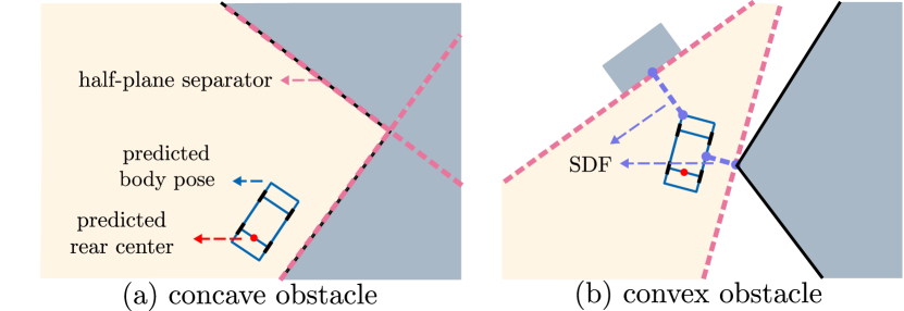
Figure 2: Illustration of how to determine the half-plane separators in the predicted states. (a) If the boundary obstacle is concave, both two lines of boundary segments are used as half-plane separators. (b) If the boundary obstacle or the random obstacle is convex, the half-plane separator is determined according to SDF.

where $\bar{A}_{k}$ and $\bar{B}_{k}$ are coefficient matrice calculated from $A_{k}$ and $B_{k}$, detailed in [39]. We now focus on specifying the collision avoidance constraint eq. 11c to enhance the robot safety while tracking the trajectory generated in algorithm 1. The linear constraints contain both the constraints of farmland boundaries and the constraints of random obstacles. First, given a predicted state vector $\boldsymbol{x}_{k+j}$ in the predicted horizon (generally written as $[x,y,\theta,v]^{T}$), we determine the boundary constraints for it in the following way, which is shown in fig. 2: first we find out the current field boundary segment $e_{i}$ (the boundary segment with minimum distance to the rear center of the vehicle) and the next boundary segment along the vehicle’s forward direction $e_{i+1}$, and determine whether the boundary obstacle formed by these two segments is convex or concave. If the boundary obstacle is concave (fig. 2(a)), the lines of the $e_{i}$ and $e_{i+1}$ are both used as half-plane separators, and the feasible region is illustrated in yellow. If the boundary obstacle is convex (fig. 2(b)), we use the Gilbert-Johnson-Keerthi (GJK) algorithm [40] and the Expanding Polytope Algorithm (EPA) [41] to find the signed distance function (SDF) $\hat{d}$ between the rectangular vehicle body and the triangle formed by $e_{i}$ and $e_{i+1}$, along with the nearest points $P_{1}$ and $P_{2}$ on the vehicle and the obstacle respectively. Then, the contact normal $\hat{n}=sgn(\hat{d})\cdot(P_{1}-P_{2})/||P_{1}-P_{2}||$ is the normal vector of the half-plane separator [42]. Second, as for the random obstacles, which we assume convex in our context, the method to determine their linear constraints is the same as in the convex case (fig. 2(b)).

For a certain half-plane separator $ax+by+c=0$ with constant $c$ and normal vector $(a,b)$ pointing towards the interior of the field. We can easily obtain the safety condition of the right front corner as:

$$ax+by +a(l\cos\theta+w\sin\theta)$$

$$+b(l\sin\theta-w\cos\theta)+c>0,$$ (18)

where $l$ is the length from the rear axis to the car front, and $w$ is half the width of the vehicle. From eq. 17 and $\tilde{\boldsymbol{X}}=\boldsymbol{X}-\boldsymbol{X}_{r}$, we know that:

$$\boldsymbol{X}_{k}=\bar{A}_{k}\tilde{\boldsymbol{x}}_{k}+\bar{B}_{k}\boldsymbol{U}_{k}+\boldsymbol{X}_{r,k}.$$ (19)

Note that $\boldsymbol{x}_{k+j}$ is obtained from eq. 19 using $\tilde{\boldsymbol{x}}_{k}$ and the control variable $\boldsymbol{U}_{k}$, and thus $\boldsymbol{x}_{k+j}$ is an unknown priori. and the nearest boundary segment is estimated using the reference trajectory $\boldsymbol{x}_{r,k+j}$ (generally written as $[x_{r},y_{r},\theta_{r},v_{r}]^{T}$). As we want to change eq. 18 into a linear inequality for $x,y$ and $\theta$, we linearly expand $sin\theta$ and $cos\theta$ at $\theta_{r}$. After simplification, the inequality can be written as:

$$\bar{C}_{k+j}\boldsymbol{x}_{k+j}<d_{k+j},$$ (20)

$$\bar{C}_{k+j}=\mathrm{diag}[a,b,c_{3},0],$$ (21)

$$c_{3}=a\left(w\cos\theta_{r}-l\sin\theta_{r}\right)+b\left(w\sin\theta_{r}+l\cos\theta_{r}\right),$$ (22)

$$d_{k+j}=-a(\sin\theta_{r}-\theta_{r}\cos\theta_{r}(\cos\theta_{r}+\theta_{r}\sin\theta_{r}-$$

$$b(\cos\theta_{r}+\theta_{r}\sin\theta_{r})+l(\sin\theta_{r}-\theta_{r}\cos\theta_{r})-c,$$ (23)

where $\bar{C}_{k+j}$ denotes the coefficient matrix and $d_{k+j}$ denotes a constant, both taking value at instant $k+j$ and predicted at instant $k$. By combining eq. 20 and eq. 19, we can obtain the linear inequality of safety constraint for the right front of the car:

$$C_{k}\boldsymbol{X}_{k}=C_{k}\left(\bar{A}_{k}\tilde{\boldsymbol{x}}_{k}+\bar{B}_{k}\boldsymbol{U}_{k}+\boldsymbol{X}_{r,k}\right)$$

$$<[d_{k+1}\enspace d_{k+2}\enspace\cdots\enspace d_{k+N}]^{T},$$ (24)

$$C_{k}=\mathrm{diag}[\bar{C}_{k+1},\bar{C}_{k+2},\cdots,\bar{C}_{k+N}].$$ (25)

Similarly, we can obtain the inequalities of safety constraints for the other three corners of the car, thus specifying the whole collision avoidance constraint eq. 11c. By applying eq. 19, eq. 13 could be solved as a constrained quadratic programming problem, which is detailed in [39].

However, although the predicted states of the linearized MPC are feasible, there are linearization errors in the predicted states, leading to risks of potential collisions in real states. Therefore, a local adjustment using nonlinear optimization is introduced:

$$\min_{\boldsymbol{u}_{k}}\quad(\boldsymbol{x}_{k+1}-\boldsymbol{x}_{r,k+1})^{T}S(\boldsymbol{x}_{k+1}-\boldsymbol{x}_{r,k+1})$$ (26)

$$\lx@cref{creftype~refnum}{eq:model2},$$ (27)

where $S$ is a coefficient matrix. On the one hand, the nonlinear optimization is dependent on the initial value, which, if chosen badly, will bring about unexpected local minimum or extensive computing time. Hence, the initial control variants solved by linearized MPC serve as good initial values, which are already close to the real state control variants, and thus are time-saving and accurate. On the other hand, the reference trajectories solved by path-tracking Hybrid A* are collision-free on the vehicle body’s scale, thus using the reference trajectories as the standard of optimization is safe. By solving eq. 26, we get the final control variant $\boldsymbol{u}_{k}$.

IV Simulation Results and Analysis

Figure 3: The five scenarios of farmland and reference path illustrations. Note that we only present 88 reference paths within a total of 713 paths.

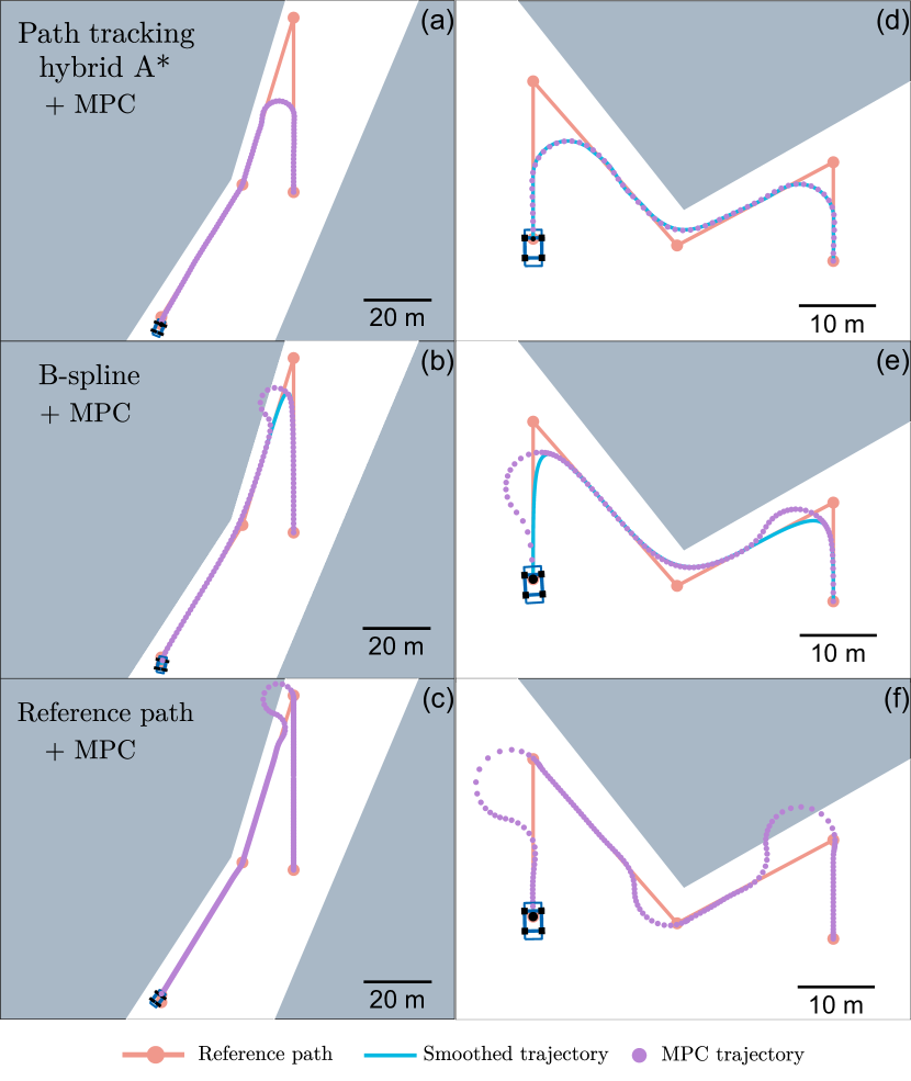
Figure 4: Comparison of three different methods on two typical scenarios. Note that each row represents experiments of the same method in different scenarios.

To evaluate the proposed algorithm, our simulation experiments are divided into three parts. First, we evaluate the path-smoothing performance of the proposed path-tracking A* algorithm (algorithm 1) in comparison with the representative collision-free B-spline path smoothing method [26]. Second, by using the MPC technique introduced in section III-E, we simulate the real furrow-crossing scenario and evaluate the success ratio and real deviation degree of MPC trajectories, to check the tracking feasibility of the smoothed trajectory and the performance of the hierarchical MPC. Third, we test the planning-control system on real-world scenarios with randomly generated obstacles, to check the obstacle avoidance ability of the planning-control system.

We conducted the simulations in five farmland scenarios, along with a total of 713 reference paths located on these farmlands, as shown in fig. 3. We should point out that the farmland and reference paths are all based on real-world data. As for the vehicle parameters, the length is 4.7m, the width is $\qty{2.2}{m}$, the wheelbase is $\qty{2.6}{m}$, and the maximum steering angle is $30^{\circ}$. As for the path-tracking A* parameters, the number of children points expanded each time is set at 5, the speed of the vehicle is $\qty{2}{m/s}$, and the interval of each expansion is $\qty{0.5}{s}$, and when encountering longer reference trajectories, we divide them into multiple shorter paths to avoid having too many points in priority queue $O$, which leads to long computation time. As for the B-spline parameters, the order of clamped B-splines is set at 3, and the midpoints of each segment are added to the reference points before generating the B-spline, since directly employing the B-spline method may yield poor performance due to sparse waypoints of the reference path. Note that here we prioritize ensuring the smoothed path is collision-free. Therefore, methods such as [25] that achieve B-spline curvature constraints by adjusting control points are not applicable in this context. The experiments are implemented in MATLAB R2023a (MathWorks, Inc.). on a laptop with an AMD Ryzen 7 5800H processor.

IV-A Evaluating Path Smoothing

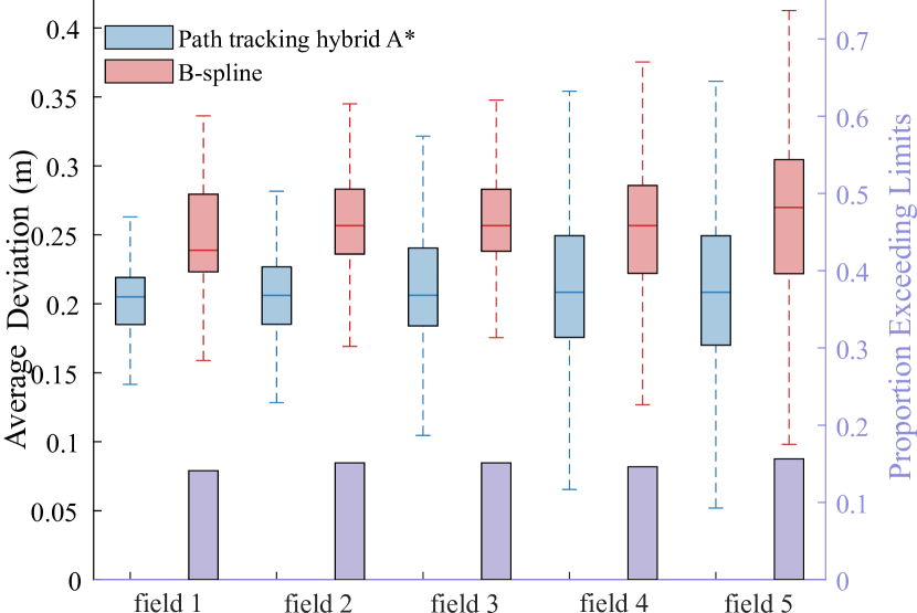
Figure 5: Average deviation degree between path-tracking Hybrid A* and the B-spline (depicted in the central box chart), and the proportion of B-spline exceeding curvature limits (shown in the lower purple bar chart).

We now focus on quantitatively evaluating the generated trajectories from two aspects, the closeness to the reference trajectory and the offset ratio of the curvature. First, We introduce the average deviation degree as a major closeness metric, which is calculated by dividing the total deviation as defined in eq. 7 by the total trajectory length:

$$E(T)=\frac{\sum_{i=1}^{n}L_{i}*dis(x_{i},R)}{\sum_{i=1}^{n}L_{i}},$$ (28)

where $T$ denotes the generated trajectory, $R$ denotes the reference trajectory, and $x_{i},i=1,2,\dots n$ are the key points of $T$.

Implementing our path tracking Hybrid A* method and the B-spline method [26], we get the statistical results of the average deviation degree and the proportion of sample points that exceeded the curvature constraints shown in the fig. 5. As seen in the box chart in fig. 5, our algorithm outperforms the B-spline method in all field scenes, owing to its explicit incorporation of the deviation degree to the cost function. Additionally, the proportion of B-spline exceeding the curvature bound is notably close to 20%, while that of path-tracking Hybrid A* stays 0%, indicating our method consistently adheres to vehicle curvature constraints whereas the B-spline method may exceed these constraints at certain points. In general, our method not only stays closer to the reference trajectory but also better satisfies curvature constraints and is easier to track by the back-end MPC, which will be further demonstrated in the next subsection.

IV-B Evaluating the MPC Trajectory Tracking Using Raw Paths and Smoothed Paths

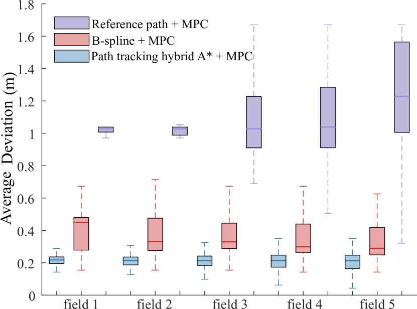
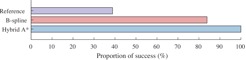
Figure 6: Average deviation degree of three different MPC trajectories.

Figure 7: Proportion of success of three different MPC trajectories.

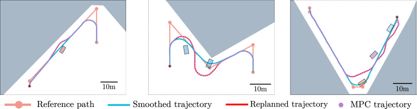
Figure 8: Typical results of the real-time obstacle avoidance of the planning-control system, under the circumstances of 1, 2, 3 random obstacles respectively.

In this section, we use the MPC method introduced in section III-E to track three kinds of paths: paths smoothed by the proposed path-tracking Hybrid A*, paths smoothed by the collision-free B-spline method[26], and the raw reference path. As smoothing results of the baseline methods don’t guarantee safety, the local adjustment of MPC is not carried out in these cases. Also, as the smoothed trajectories generated by baseline methods yield poor tracking feasibility, rendering the optimization problem eq. 11a unsolvable some cases, we adopt a unified method: when an unsolvable situation occurs, we remove the constraint eq. 11c and implement a collision detection after each track to evaluate the safety of the robot trajectory. We set the prediction horizon of MPC at 20, and we define failure as occurring under the following conditions: when the vehicle collides with obstacles, or when the vehicle ends up with a distance greater than 10m from the endpoint or with an angle greater than $60^{\circ}$ relative to the endpoint, since the vehicle is constrained in direction when entering a furrow.

The tracking trajectories in typical scenarios are presented in fig. 4. For the raw reference path, the vehicle is confronted with sharp turning angles with infinite curvature at the turning point, which makes it tough for MPC to track. Therefore, the vehicle is unable to follow the reference path closely, resulting in notable deviation which leads to failure, as shown in fig. 4. As for the B-spline case, the curvature at turning angles is smaller but still exceeds the curvature limit of the vehicle at some points, which leads to less large deviation and corresponding failure as well. On the other hand, our method generates trajectories close to the reference path which always conform to the vehicle’s nonholonomic constraints, and can be tracked by MPC smoothly without collision.

The deviation degree and the proportion of successful tracking are presented in fig. 7 and fig. 7. From fig. 7 it is easily observed that our path-tracking Hybrid A* path smoothing algorithm has a better closeness to the reference path in the simulation, and in fig. 7 we can read that our algorithm is perfectly safe, and trackable on all the reference paths in the simulation test. In comparison, the MPC result of the B-spline method and the raw reference path have a larger deviation and a lower proportion of success. Besides, the computing time of MPC has been recorded, which has an average of 0.0366s and a variance of 8.7e-5, proving our hierarchical MPC has an acceptable computational speed.

IV-C Test on Real-Time Obstacle Avoidance

TABLE I: statistical results of real-time obstacle avoidance

number of obstacles		1	2	3
success ratio		100%	98.8%	97.4%
replanning time (s)	mean	0.6449	0.6713	0.7782
	variance	0.2639	0.4138	0.7668
control time (s)	mean	0.0518	0.0733	0.0990
	variance	5.0e-4	0.0011	0.0024

This section exhibits the test results of the real-time obstacle avoidance performance of the planning-control system. To carry out the experiments, we chose 10 typical reference paths, and randomly set rectangular obstacles around the reference path. The width and height of the obstacles are set at 2m and 4m, which is almost the size of an agricultural vehicle. The detection range of the vehicle is set at 15m, and the FOV is set at $90^{\circ}$. For each obstacle number that ranges from 1 to 3, we fix the number of obstacles and test 50 cases in each scenario, and in each case, the obstacles are randomly generated. Note that occasions where the obstacles block the start pose or the end pose are excluded. Some typical trajectories are shown in fig. 8, and the statistical results are shown in table I. From fig. 8, we can see that the trajectories replanned by path-tracking Hybrid A* are close to the original smoothed trajectories, and can be smoothly connected with other parts of the original trajectories. Besides, the hierarchical MPC allows the vehicle to safely track the replanned trajectories, even through the narrow passages.

From table I, we can see that due to the increasing obstacle density and the narrowing of the feasible paths, the failure ratio, planning time, and control time gradually increase as the number of obstacles grows. However, in general, our planning-control system has high success ratios, planning speeds, and control speeds under 1-3 obstacles.

V Conclusion

We propose a path-tracking Hybrid A* planner and a coupled hierarchical MPC controller for the path smoothing of agricultural vehicles. We devise new cost and heuristic functions to minimize the deviation degree. The proposed planning-control system results in smooth and obstacle-free trajectories for agricultural vehicles, both in offline and real-time scenarios, as shown in the experiments on real-world farm datasets. Future directions include either the whole field path planning, to achieve maximum field coverage in addition to the minimum deviation, or the multi-vehicle collaboration, to allocate the tasks of agricultural operations to each vehicle with the minimum total deviation.

References

- [1] V. Moysiadis, N. Tsolakis, D. Katikaridis, C. G. Sørensen, S. Pearson, and D. Bochtis, “Mobile robotics in agricultural operations: A narrative review on planning aspects,” Applied Sciences, vol. 10, no. 10, p. 3453, 2020.
- [2] D. Zhang, C. Chen, and G. Zhang, “Agv path planning based on improved a-star algorithm,” in 2024 IEEE 7th Advanced Information Technology, Electronic and Automation Control Conference (IAEAC), vol. 7, pp. 1590–1595, 2024.
- [3] D. Dolgov, S. Thrun, M. Montemerlo, and J. Diebel, “Practical search techniques in path planning for autonomous driving,” Ann Arbor, vol. 1001, no. 48105, pp. 18–80, 2008.
- [4] H. Tu, Y. Deng, Q. Li, M. Song, and X. Zheng, “Improved rrt global path planning algorithm based on bridge test,” Robotics and Autonomous Systems, vol. 171, p. 104570, 2024.
- [5] L. E. Kavraki, M. N. Kolountzakis, and J.-C. Latombe, “Analysis of probabilistic roadmaps for path planning,” IEEE Transactions on Robotics and automation, vol. 14, no. 1, pp. 166–171, 1998.
- [6] P. Qin, F. Liu, Z. Guo, Z. Li, and Y. Shang, “Hierarchical collision-free trajectory planning for autonomous vehicles based on improved artificial potential field method,” Transactions of the Institute of Measurement and Control, vol. 46, no. 4, pp. 799–812, 2024.
- [7] L. C. Santos, F. N. Santos, E. S. Pires, A. Valente, P. Costa, and S. Magalhães, “Path planning for ground robots in agriculture: A short review,” in 2020 IEEE International Conference on Autonomous Robot Systems and Competitions (ICARSC), pp. 61–66, 2020.
- [8] L. Santos, F. Santos, J. Mendes, P. Costa, J. Lima, R. Reis, and P. Shinde, “Path planning aware of robot’s center of mass for steep slope vineyards,” Robotica, vol. 38, no. 4, pp. 684–698, 2020.
- [9] T. Mai, S. Shao, and Z. Yun, “The path planning of agricultural agv in potato ridge cultivation,” Ann. Adv. Agric. Sci, vol. 3, no. 2, 2019.
- [10] I. A. Hameed, “Intelligent coverage path planning for agricultural robots and autonomous machines on three-dimensional terrain,” Journal of Intelligent & Robotic Systems, vol. 74, no. 3, pp. 965–983, 2014.
- [11] M. M. Rahman, K. Ishii, and N. Noguchi, “Optimum harvesting area of convex and concave polygon field for path planning of robot combine harvester,” Intelligent service robotics, vol. 12, pp. 167–179, 2019.
- [12] C. S. Tan, R. Mohd-Mokhtar, and M. R. Arshad, “A comprehensive review of coverage path planning in robotics using classical and heuristic algorithms,” IEEE Access, vol. 9, pp. 119310–119342, 2021.
- [13] X.-T. Yan, A. Bianco, C. Niu, R. Palazzetti, G. Henry, Y. Li, W. Tubby, A. Kisdi, R. Irshad, S. Sanders, et al., “The agrirover: a reinvented mechatronic platform from space robotics for precision farming,” Reinventing Mechatronics: Developing Future Directions for Mechatronics, pp. 55–73, 2020.
- [14] S. Sedighi, D.-V. Nguyen, and K.-D. Kuhnert, “Guided hybrid a-star path planning algorithm for valet parking applications,” in 2019 5th international conference on control, automation and robotics (ICCAR), pp. 570–575, 2019.
- [15] W. Sheng, B. Li, and X. Zhong, “Autonomous parking trajectory planning with tiny passages: A combination of multistage hybrid a-star algorithm and numerical optimal control,” IEEE Access, vol. 9, pp. 102801–102810, 2021.
- [16] H. Zheng, M. Dai, Z. Zhang, Z. Xia, G. Zhang, and F. Jia, “The navigation based on hybrid a star and teb algorithm implemented in obstacles avoidance,” in 2023 29th International Conference on Mechatronics and Machine Vision in Practice (M2VIP), pp. 1–6, 2023.
- [17] T. Chang and G. Tian, “Hybrid a-star path planning method based on hierarchical clustering and trichotomy,” Applied Sciences, vol. 14, no. 13, p. 5582, 2024.
- [18] T. Meng, T. Yang, J. Huang, W. Jin, W. Zhang, Y. Jia, K. Wan, G. Xiao, D. Yang, and Z. Zhong, “Improved hybrid a-star algorithm for path planning in autonomous parking system based on multi-stage dynamic optimization,” International journal of automotive technology, vol. 24, no. 2, pp. 459–468, 2023.
- [19] A. Ravankar, A. A. Ravankar, Y. Kobayashi, Y. Hoshino, and C.-C. Peng, “Path smoothing techniques in robot navigation: State-of-the-art, current and future challenges,” Sensors, vol. 18, no. 9, p. 3170, 2018.
- [20] J. F. Epperson, “On the runge example,” The American Mathematical Monthly, vol. 94, no. 4, pp. 329–341, 1987.
- [21] K. Yang and S. Sukkarieh, “An analytical continuous-curvature path-smoothing algorithm,” IEEE Transactions on Robotics, vol. 26, no. 3, pp. 561–568, 2010.
- [22] K. Kawabata, L. Ma, J. Xue, C. Zhu, and N. Zheng, “A path generation for automated vehicle based on bezier curve and via-points,” Robotics and Autonomous Systems, vol. 74, pp. 243–252, 2015.
- [23] Z. Duraklı and V. Nabiyev, “A new approach based on bezier curves to solve path planning problems for mobile robots,” Journal of computational science, vol. 58, p. 101540, 2022.
- [24] X. Liu, H. Nie, D. Li, Y. He, and M. H. Ang, “High-fidelity and curvature-continuous path smoothing with quadratic bézier curve,” IEEE Transactions on Intelligent Vehicles, 2024.
- [25] M. Elbanhawi, M. Simic, and R. N. Jazar, “Continuous path smoothing for car-like robots using b-spline curves,” Journal of Intelligent & Robotic Systems, vol. 80, pp. 23–56, 2015.
- [26] I. Noreen, “Collision free smooth path for mobile robots in cluttered environment using an economical clamped cubic b-spline,” Symmetry, vol. 12, no. 9, p. 1567, 2020.
- [27] X. Li, X. Gao, W. Zhang, and L. Hao, “Smooth and collision-free trajectory generation in cluttered environments using cubic b-spline form,” Mechanism and Machine Theory, vol. 169, p. 104606, 2022.
- [28] S. Havemann, J. Edelsbrunner, P. Wagner, and D. Fellner, “Curvature-controlled curve editing using piecewise clothoid curves,” Computers & Graphics, vol. 37, no. 6, pp. 764–773, 2013.
- [29] E. D. Lambert, R. Romano, and D. Watling, “Optimal smooth paths based on clothoids for car-like vehicles in the presence of obstacles,” International Journal of Control, Automation and Systems, vol. 19, pp. 2163–2182, 2021.
- [30] P. Lin, E. Javanmardi, and M. Tsukada, “Clothoid curve-based emergency-stopping path planning with adaptive potential field for autonomous vehicles,” IEEE Transactions on Vehicular Technology, 2024.
- [31] L. E. Dubins, “On curves of minimal length with a constraint on average curvature, and with prescribed initial and terminal positions and tangents,” American Journal of mathematics, vol. 79, no. 3, pp. 497–516, 1957.
- [32] J. Reeds and L. Shepp, “Optimal paths for a car that goes both forwards and backwards,” Pacific journal of mathematics, vol. 145, no. 2, pp. 367–393, 1990.
- [33] S. Park, “Three-dimensional dubins-path-guided continuous curvature path smoothing,” Applied Sciences, vol. 12, no. 22, p. 11336, 2022.
- [34] L. Xu, D. Wang, B. Song, and M. Cao, “Global smooth path planning for mobile robots based on continuous bezier curve,” in 2017 Chinese Automation Congress (CAC), pp. 2081–2085, 2017.
- [35] B. Song, Z. Wang, and L. Zou, “An improved pso algorithm for smooth path planning of mobile robots using continuous high-degree bezier curve,” Applied soft computing, vol. 100, p. 106960, 2021.
- [36] L. Xu, M. Cao, and B. Song, “A new approach to smooth path planning of mobile robot based on quartic bezier transition curve and improved pso algorithm,” Neurocomputing, vol. 473, pp. 98–106, 2022.
- [37] K. Feng, X. He, M. Wang, X. Chu, D. Wang, and D. Yue, “Path optimization of agricultural robot based on immune ant colony: B-spline interpolation algorithm,” Mathematical Problems in Engineering, vol. 2022, no. 1, p. 2585910, 2022.
- [38] F. Huo, S. Zhu, H. Dong, and W. Ren, “A new approach to smooth path planning of ackerman mobile robot based on improved aco algorithm and b-spline curve,” Robotics and Autonomous Systems, vol. 175, p. 104655, 2024.
- [39] F. Künhe, J. Gomes, and W. Fetter, “Mobile robot trajectory tracking using model predictive control,” in II IEEE latin-american robotics symposium, vol. 51, p. 5, 2005.
- [40] E. G. Gilbert, D. W. Johnson, and S. S. Keerthi, “A fast procedure for computing the distance between complex objects in three-dimensional space,” IEEE Journal on Robotics and Automation, vol. 4, no. 2, pp. 193–203, 1988.
- [41] G. Van Den Bergen, “Proximity queries and penetration depth computation on 3d game objects,” in Game developers conference, vol. 170, p. 209, 2001.
- [42] H. Gao, W. Pengying, S. Yao, K. Zhou, M. Ji, H. Liu, and C. Liu, “Probabilistic visibility-aware trajectory planning for target tracking in cluttered environments,” in 2024 American Control Conference (ACC), pp. 594–600, 2024.