Neural numerical homogenization based on Deep Ritz corrections

Abstract.

Numerical homogenization methods aim at providing appropriate coarse-scale approximations of solutions to (elliptic) partial differential equations that involve highly oscillatory coefficients. The localized orthogonal decomposition (LOD) method is an effective way of dealing with such coefficients, especially if they are non-periodic and non-smooth. It modifies classical finite element basis functions by suitable fine-scale corrections. In this paper, we make use of the structure of the LOD method, but we propose to calculate the corrections based on a Deep Ritz approach involving a parametrization of the coefficients to tackle temporal variations or uncertainties. Numerical examples for a parabolic model problem are presented to assess the performance of the approach.

Keywords. parabolic equation, numerical homogenization, multiscale method, Deep Ritz method

Mathematics Subject Classification. 65M60, 35K20, 68T07

1. Introduction

Composite materials play an important role in modern technologies, as they enable the combination of complex properties such as high strength, lightweight, thermal resistance, and electrical conductivity- characteristics that are often unattainable with plain homogeneous materials. A notable example for their application can be found in batteries. An interesting question in this context is the study of the thermal behavior of the cell during the charging/discharging protocol, especially during fast charging, where increased voltages and currents can lead to thermal breakdowns if not properly monitored and controlled. In the most simple manner, the temperature in a battery cell can be modeled by a parabolic equation (similar to [Ves22]). More precisely, we seek the heat distribution $u$ that solves

(1) $$\partial_{t}u(x,t)-\operatorname{div}(a(x,t)\nabla u(x,t))=f(x,t),\qquad x\in\Omega,\quad t\in[0,T],$$

where $\Omega$ is an open bounded domain, $T$ the final time, $a$ a given heat conductivity coefficient, and $f$ a heat source. Note that $a$ is oscillatory in space and may change over time. In particular, battery cells usually consist of a large amount of layers that have very small widths $\varepsilon$. This multiscale structure makes the simulation using standard methods, such as the finite element method (FEM), inherently expensive. If $\varepsilon$ is not resolved by the mesh parameter, the solution behaves badly even if only macroscopic approximation properties are of interest. Therefore, very fine meshes are necessary to obtain reasonable results (this is also known as the pre-asymptotic behavior of the FEM). Thus, reducing the computational complexity with tailor-made multiscale methods is highly beneficial. Under additional assumptions on the coefficient $a$ (such as periodicity and scale separation in [Ves22]), the use of multiscale methods based on analytical homogenization theory are an appropriate and efficient choice. The method applied by [Ves22] is the heterogeneous multiscale method (HMM), which has first been introduced in the elliptic setting in [EE03, EE05] (see also [AEEV12]). The methodology has since then been applied to various parabolic and parabolic-type problems, see, e.g., [MZ07, AV12, Abd16, AH17]. It may also be used to tackle highly oscillatory coefficients in space and time and stochastic partial differential equations (PDEs), see [EV23] and [AP12], respectively. The HMM calculates a coarse system matrix by approximating the homogenized coefficient from analytical homogenization theory. The system is then used to compute a coarse approximation of the (homogenized) solution to the original PDE. Another approach is the multiscale finite element method, see [HW97, AB05], which corrects coarse basis functions by solving operator-adapted problems in each element of the mesh. The corresponding analysis is based on analytical homogenization theory as well, which again requires structural assumptions.

In practice, the structure of materials in batteries is more involved, specifically the so-called active material is usually strongly heterogeneous as well as non-periodic. This promotes the use of more general approaches, so-called numerical homogenization techniques that provably work under minimal assumptions on the coefficient. A starting point for further developments has been the variational multiscale method introduced in [Hug95, HFMQ98], which decomposes the problem into an equation for a coarse-scale and a fine-scale function, respectively, and appropriately includes fine-scale information into the coarse-scale equation. Further strategies include rough polyharmonic splines [OZB14], where basis functions are constructed based on a constrained minimization of the PDE operator in the $L^{2}$-norm, or gamblets [Owh17, OS19], where the energy of basis functions is minimized. Gamblets are introduced based on a game theoretic approach to multiscale problems and have been applied to parabolic PDEs in [OZ17]. Other approaches under minimal assumptions are generalized (multiscale) finite element methods [BL11, EGH13, MS22, MSD22] that build basis functions based on locally solving spectral problems. For a more in-depth overview of multiscale methods, we refer to [AHP21] and the textbooks [OS19, MP20].

The multiscale setting including space- and time-dependent coefficients poses difficult questions since the above-mentioned approaches require an update of the spatial approximation spaces at a relatively high cost. Methods that work around this bottleneck are thus vital and examples dealing with this question employing space-time approaches include an approach by [OZ08], where the basis functions of the ansatz and test space are subject to a global harmonic transform, or the high-dimensional sparse finite element method in [TH19], which requires a clear scale separation of the coefficient. The construction of optimal local subspaces based on the generalized finite element method for space-time coefficients is analyzed in [SS22, SSTM23]. Another space-time multiscale method based on the generalized multiscale finite element method is considered in [CELY18].

The proposed method in this paper is based on the localized orthogonal decomposition (LOD) method introduced in [MP14, HP13] (see also [MP20]), that constructs an appropriate orthogonal decomposition of an ideal approximation space and remaining fine-scale functions. The ideal approximation space can be well-approximated by correcting classical coarse-scale finite element functions on a chosen scale $H>\varepsilon$ with the solutions to local auxiliary problems (so-called corrections). The LOD method provably works under very general assumptions on the coefficient $a$, which makes it fitting to our problem. The approach has previously been applied to parabolic PDEs in [MP18] and to coupled elliptic-parabolic problems in [MP17, ACM⁺20]. The LOD method is particularly well-suited for time-dependent problems, where the modified approximation space is built in an offline phase. A substantial speedup is then achieved in the online phase when iterating through time as the resulting system matrices are of moderate size only. The offline phase where the LOD basis functions are set up is the bottleneck of the method. If the coefficient changes in time, substantial re-computations of the approximation space are necessary such that the method loses its efficiency in the online phase. In [LMM22] the time-dependence was tackled by posing the LOD method in a space-time setting. Here, we stick to the idea of updating the approximation spaces but we avoid expensive re-computations by employing an appropriate trained artificial neural network (ANN) that realizes the corrections and is parametrized by the coefficient. This allows for quick updates once the coefficient has changed and an adjustment is necessary. Such a strategy is also useful if the specific heat conductivity is not known a priori and only an approximate expected solution may be computed. Note that the possibility to quickly obtain modified basis functions for a plethora of coefficients eventually makes up for the training phase and therefore provides a valuable enhancement of the LOD method for the setting of space-time oscillatory coefficients.

The paper is structured as follows. In Section 2, we establish the parabolic model problem considered in this paper and introduce the basics of the LOD method as the spatial discretization technique. In Section 3, we explain how to compute the Deep Ritz-based corrections, which are eventually used to set up a modified LOD approach. Finally, we present numerical examples in Section 4.

2. Numerical Homogenization by Localized Orthogonal Decomposition

2.1. Model problem

Recall that we aim at (approximately) solving parabolic PDEs of the form (1). More precisely, for a bounded Lipschitz domain $\Omega\subset{\mathbb{R}}^{d}$ ($d=1,2,3$) with boundary $\Gamma\coloneqq\partial\Omega$ and a final time $T>0$, we seek a function $u$ such that

(2) $$\partial_{t}u-\operatorname{div}(a\nabla u) =f \quad\mathrm{in}\leavevmode\nobreak\ \Omega\times(0,T],$$

$$u =g \quad\mathrm{on}\leavevmode\nobreak\ \Gamma\times(0,T],$$

$$u =u_{0} \quad\mathrm{in}\leavevmode\nobreak\ \Omega\times\{0\},$$

with an appropriate source term $f$, boundary function $g$, and initial condition $u_{0}$, where the coefficient $a\in L^{\infty}(0,T;L^{\infty}(\Omega))$ might vary in space and time and satisfies $0<\alpha\leq a(x,t)\leq\beta<\infty$ for a.a. $x\in\Omega$ and $t\in[0,T]$. We note that $a$ could also be matrix-valued but for simplicity we focus on scalar coefficients only. Here, we have coefficients in mind that vary in space on a fine scale $0<\varepsilon\ll 1$ and possibly in time as well. Furthermore, the coefficient $a$ could inherit some form of uncertainty in the sense that on a subset $\omega\subset\Omega$ the coefficient might not be known exactly except for upper and lower bounds. In the following, we only consider the case $g\equiv 0$ for simplicity. The variational formulation of (2) then seeks $u\in L^{2}(0,T;H_{0}^{1}(\Omega))\cap H^{1}(0,T;H^{-1}(\Omega))$ that solves

(3) $$\langle\partial_{t}u,v\rangle+\mathfrak{A}(u,v) =\int_{\Omega}fv\,\mathrm{d}x$$

for all $v\in H_{0}^{1}(\Omega)$, where

$$\langle w,v\rangle\coloneqq w(v)$$

for $w\in H^{-1}(\Omega)$ and $v\in H^{1}_{0}(\Omega)$ denotes the corresponding duality pairing, and

(4) $$\mathfrak{A}(w,v):=\int_{\Omega}a\nabla w\cdot\nabla v\,\mathrm{d}x$$

for $w,v\in H_{0}^{1}(\Omega)$ denotes the $a$-induced inner product on $H_{0}^{1}(\Omega)$. Note that $\mathfrak{A}$ may depend on time through the coefficient $a$.

2.2. Localized orthogonal decomposition

The LOD method [MP14, HP13, MP20] constructs a coarse-scale problem-adapted approximation space based on the bilinear form (4). In this subsection, we introduce the basics of the approach and then modify it based on a Deep Ritz ansatz in the following section. The overall goal of this modification will be to leverage generalization properties of neural networks to quickly update the approximation space when coefficients change over time.

Let $\mathcal{T}_{H}$ be a quasi-uniform, quadrilateral mesh with mesh size $H>\varepsilon$ and let $V_{H}$ be the conforming subspace of $H_{0}^{1}(\Omega)$ defined by

(5) $$V_{H}\coloneqq\{v\in C^{0}(\Omega)\mid\forall K\in\mathcal{T}_{H}\colon v|_{K}\text{ is a polynomial of partial degree}\leq 1\}\subset H_{0}^{1}(\Omega)$$

We denote with $\{\Lambda_{j}\}_{j=1}^{N_{H}}$, where $N_{H}=\dim V_{H}$, the classical nodal basis of $V_{H}$. Further, we need an appropriate quasi-interpolation operator onto $V_{H}$, which is introduced in the following.

Definition 2.1 (Patch).

Let $\ell\geq 1$ and $S\subseteq\Omega$. Define the patch (of order $\ell$) around $S$ by the recursion $\mathsf{N}^{\ell+1}(S)=\mathsf{N}(\mathsf{N}^{\ell}(S))$ with $\mathsf{N}^{1}(S):=\mathsf{N}(S)$ and

$$\mathsf{N}(S):=\bigcup\bigl{\{}\overline{K}\in\mathcal{T}_{h}\,|\,\overline{S}\,\cap\,\overline{K}\neq\emptyset\bigl{\}}.$$

Definition 2.2 (Local projective quasi-interpolation operator).

The operator $\mathcal{I}_{H}\colon L^{2}(\Omega)\to V_{H}$ is called local projective quasi-interpolation operator, if it is a projection, i.e., $\mathcal{I}_{H}\circ\mathcal{I}_{H}=\mathcal{I}_{H}$, and stable in the sense of

(6) $$H^{-1}\|v-\mathcal{I}_{H}v\|_{L^{2}(K)}+\|\nabla\mathcal{I}_{H}v\|_{L^{2}(K)}\leq C\|\nabla v\|_{L^{2}(\mathsf{N}(K))}$$

for all $K\in\mathcal{T}_{H}$ and all $v\in H_{0}^{1}(\Omega)$, where the constant $C$ is independent of $H$.

A classical choice for such a quasi-interpolation operator, which is used in our numerical experiments, is constructed in the following. We set

(7) $$\mathcal{I}_{H}:=\pi_{H}\circ\Pi^{\textrm{dg}}_{H},$$

where $\Pi^{\textrm{dg}}_{H}$ denotes the $L^{2}$-projection onto the space

$$V_{H}^{\textrm{dg}}\coloneqq\{v\in L^{2}(\Omega)\mid\forall K\in\mathcal{T}_{H}\colon v|_{K}\text{ is a polynomial of partial degree}\leq 1\},$$

and $\pi_{H}$ is an averaging operator from $V_{H}^{\textrm{dg}}$ to $V_{H}$ that assigns to each inner vertex the arithmetic mean of the corresponding function values of the neighboring elements. To all boundary vertices $z\in\Gamma$ the value zero is assigned. More precisely, for any $v_{H}\in V_{H}^{\textrm{dg}}$, $\pi_{H}(v_{H})$ is characterized by

$$\big{(}\pi_{H}(v_{H})\big{)}(z):=\sum_{K\in\mathcal{T}_{H}\colon z\in\overline{K}}\big{(}{v_{H}|}_{K}\big{)}(z)\cdot\frac{1}{\mathrm{card}\{G\in\mathcal{T}_{H}\,\colon\,z\in\overline{G}\}}$$

for all vertices $z$ of $\mathcal{T}_{H}$ with $z\notin\Gamma$. The operator $\mathcal{I}_{H}$ fulfills the properties of Definition 2.2, see, e.g., [EG17].

The space $V_{H}$ is not able to capture fine oscillations of functions that lie in the so-called fine-scale space $\mathcal{W}:=\ker\mathcal{I}_{H}|_{H_{0}^{1}(\Omega)}$. Therefore, the main idea of the LOD method is to suitably enrich the basis functions $\Lambda_{j}$ of $V_{H}$ by functions in the space $\mathcal{W}$. We obtain the fine-scale information by the prototypical (globally defined) correction from the correction operator $\mathcal{C}\colon H_{0}^{1}(\Omega)\to\mathcal{W}$ defined for any $v\in H_{0}^{1}(\Omega)$ and a fixed time $t$ by

(8) $$\mathfrak{A}(\mathcal{C}v,w)=\mathfrak{A}(v,w)$$

for all $w\in\mathcal{W}$. The prototypical multiscale space is given by $({\operatorname{Id}}-\mathcal{C})V_{H}\eqqcolon\widetilde{V}_{H}$ with basis $\{\widetilde{\Lambda}_{j}\}_{j=1}^{N_{H}}$, where $\widetilde{\Lambda}_{j}:=({\operatorname{Id}}-\mathcal{C})\Lambda_{j}$. Note that this space may change over time if $a$ is time-dependent. With this construction, the basis function $\widetilde{\Lambda}_{j}$, $j=1,\ldots,N_{H}$ is in general globally defined, but it can be shown that it decays exponentially away from the support of the corresponding nodal basis function $\Lambda_{j}$. This means if we were to localize each $\widetilde{\Lambda}_{j}$ on a sufficiently large subdomain of $\Omega$, we would only make a relatively small error. For a rigorous definition of the localization we first introduce for any $K\in\mathcal{T}_{H}$ the element-wise correction operator $\mathcal{C}_{K}\colon H_{0}^{1}(\Omega)\to\mathcal{W}$, which is defined for any $v\in H_{0}^{1}(\Omega)$ by

(9) $$\mathfrak{A}(\mathcal{C}_{K}v,w)=\mathfrak{A}|_{K}(v,w),$$

for all $w\in\mathcal{W}$, where $\mathfrak{A}|_{K}(v,w)\coloneqq\int_{K}a\nabla v\cdot\nabla w\,\mathrm{d}x$ is the restriction of the inner product to an element $K$. Then we have $\mathcal{C}=\sum_{K\in\mathcal{T}_{H}}\mathcal{C}_{K}$. Employing these element-wise corrections we can introduce a localization to patches on the left-hand side of (9) as defined in the following.

Definition 2.3 (Localized correction operator).

Let $\ell\geq 1$ and $K\in\mathcal{T}_{H}$. Further, let $\mathcal{W}(\mathsf{N}^{\ell}(S))$ the space of functions $v\in\mathcal{W}$ with $\operatorname{supp}v\subset\mathsf{N}^{\ell}(S)$. The localized element-wise correction operator $\mathcal{C}_{K}^{\ell}\colon H_{0}^{1}(\Omega)\to\mathcal{W}(\mathsf{N}^{\ell}(K))$ is defined for any $v\in H_{0}^{1}(\Omega)$ by

(10) $$\mathfrak{A}(\mathcal{C}_{K}^{\ell}v,w)=\mathfrak{A}|_{K}(v,w),$$

for all $w\in\mathcal{W}(\mathsf{N}^{\ell}(K))$. The localized correction operator is defined as the sum $\mathcal{C}^{\ell}=\sum_{K\in\mathcal{T}_{H}}\mathcal{C}_{K}^{\ell}$.

Definition 2.4 (Localized multiscale space).

We define the localized multiscale space as

$$\widetilde{V}_{H}^{\ell}=({\operatorname{Id}}-\mathcal{C}^{\ell})V_{H}.$$

A basis of $\widetilde{V}_{H}^{\ell}$ is given by $\{\widetilde{\Lambda}_{j}^{\ell}\}_{j=1}^{N_{H}}$ with $\widetilde{\Lambda}_{j}^{\ell}\coloneqq({\operatorname{Id}}-\mathcal{C}^{\ell})\Lambda_{j}$ for all basis functions $\Lambda_{j}$ of $V_{H}$.

Note that the left-hand side of (10) is restricted to a single patch $\mathsf{N}^{\ell}(K)$. To avoid the explicit characterization (including a basis) of $\mathcal{W}$, the correction operator $\mathcal{C}_{K}^{\ell}$ may also equivalently be defined as a minimization problem. As we only require knowledge of the functions $\widetilde{\Lambda}_{j}^{\ell}$, it suffices to calculate the element contributions of the nodal basis functions $\Lambda_{j}$ of $V_{H}$. For $\ell\geq 1$, the equivalent constrained minimization problem seeks for any $j=1,\dots,N_{H}$ and any $K\in\mathcal{T}_{H}$ the unique minimizer

(11) $$\mathcal{C}_{K}^{\ell}\Lambda_{j}=\operatorname*{argmin}_{v\in H_{0}^{1}(\mathsf{N}^{\ell}(K))}\frac{1}{2}\int_{\mathsf{N}^{\ell}(K)}a\nabla v\cdot\nabla v\,\mathrm{d}x-\int_{K}a\nabla\Lambda_{j}\cdot\nabla v\,\mathrm{d}x\quad\mathrm{s.t.}\quad\mathcal{I}_{H}v=0.$$

Thus, we obtain a basis of $\widetilde{V}_{H}^{\ell}$ by

(12) $$\widetilde{\Lambda}_{j}^{\ell}=\Lambda_{j}-\sum_{K\in\mathcal{T}_{H}}\mathcal{C}_{K}^{\ell}\Lambda_{j}=\Lambda_{j}-\sum_{K\in\mathcal{T}_{H}\colon\operatorname{supp}(\Lambda_{j})\cap K\neq\emptyset}\mathcal{C}_{K}^{\ell}\Lambda_{j}.$$

The representation (11) is well-suited for the usage as a loss functional within a Deep Ritz framework as introduced in [EY18]. If trained including a parametrization of the local coefficient $a|_{\mathsf{N}^{\ell}(K)}$ (more information on the parametrization is presented in Section 2.3) we obtain a strategy to quickly access the localized correction for an element $K$ once a specific coefficient is given. This makes it possible to avoid costly re-computations if the coefficient changes over time or if multiple coefficients are accounted for as it is the case in the presence of uncertainties.

Figure 1. Examples of possible patch configurations

At this point, we have only explained the construction of the LOD multiscale space but not yet given any error bounds. The advantage of the LOD method is that the pre-asymptotic behavior of the FEM can be overcome, and we can solve equations on the coarse mesh $\mathcal{T}_{H}$ that provide good approximations to the exact solution. This is summarized in the theorem below based on [MP20, Ch. 5]. Let $\widetilde{u}_{H}\in\widetilde{V}_{H}^{\ell}$ be the LOD solution and $u\in H_{0}^{1}(\Omega)$ be the weak solution, respectively, to

(13) $$\mathfrak{A}(\widetilde{u}_{H},\widetilde{v}_{H}) =\int_{\Omega}f\widetilde{v}_{H}\,\mathrm{d}x,$$

$$\mathfrak{A}(u,v) =\int_{\Omega}fv\,\mathrm{d}x,$$

for all $\widetilde{v}_{H}\in\widetilde{V}_{H}^{\ell}$ and for all $v\in H_{0}^{1}(\Omega)$. We note that if $f\in H^{-1}(\Omega)$ there exist unique solutions to the two variational problems in (13), respectively, by the Lax-Milgram theorem, cf., e.g., [BS08, Ch. 2].

Theorem 2.5 (Error of the LOD method).

Let $\widetilde{u}_{H}$ and $u$ be the solutions to (13), respectively. Then the error bound reads as follows:

(14) $$\|\nabla(\widetilde{u}_{H}-u)\|_{L^{2}(\Omega)}\leq C(H+e_{\mathrm{loc}}),$$

where the constant $C>0$ is independent of $H$, $\ell$ and $\varepsilon$, but depends on the norm of $f$ and the contrast $\frac{\beta}{\alpha}$ of the coefficient $a$. Here, $e_{\textrm{loc}}$ denotes the localization error.

For the localization error $e_{\textrm{loc}}$ it holds

(15) $$e_{\mathrm{loc}}\leq C_{\textrm{loc}}\ell^{\frac{d}{2}}\operatorname{exp}(-C_{\textrm{d}}\ell),$$

where $C_{\textrm{loc}}$ and $C_{\textrm{d}}$ are independent of $H$ and $\ell$. If we now choose $\ell\approx|\log H|$, we preserve the convergence rate $H$ of the non-localized method. A complete error analysis can be found in [MP20, Ch. 4 & 5].

We emphasize that the error estimates consider the elliptic setting only. For time-dependent problems, these estimates can still be used to bound the projection error into the LOD space. For parabolic equations with time-independent coefficient, a fully discrete error analysis can then be derived as in [MP18].

2.3. Parametrizing the coefficient

Before we provide the application of ANNs to learn problem-adapted basis functions, we give some notes on the advancements we are trying to achieve. The LOD method performs optimally in the setting of the parabolic equation (2) where the modeled material, i.e., the coefficient, is constant over time. In this case, the multiscale space is time-independent and the calculation of the corrections can be carried out once in parallel in a pre-processing step which results in very fast time propagation by classical time stepping methods due to the vast reduction of numbers of degrees of freedom. This advantage is lost if the coefficient contains fast variations in time. In this case, the multiscale space needs to be adjusted with time. This comes at a large cost, and additional ideas are necessary. Possible solutions include using space-time ansatz functions as in [LMM22], or using an error estimator to only partially update the spaces similar as in [HM19, HKM20, MV22]. Our approach aims at leveraging two main advantages of neural networks. The first one is their generalization property, in the sense that we can train the network for some set of coefficients and then obtain the basis functions through a simple forward-pass, even if the coefficient was not in the training set. The second advantage is that this forward-pass is rather cheap and can be done online within each time step. Such an approach is also advantageous if no exact a priori knowledge of the coefficient is known, but rather a broad guess on the range of possible coefficients. In this setting, we might need to compute a plethora of correction problems to estimate, e.g., the expectation, see for instance [GP19, FGP21, HMP24]. There, it can be beneficial to quickly obtain the corrections and basis functions as cheap forward-passes through the network.

Coming back to the assumptions on the coefficient in Section 2.1, we parametrize the coefficient as $a(x,\mathbf{p})$, where $\mathbf{p}$ parametrizes the coefficient to allow for, e.g., a time-dependence or uncertainty.

3. Approximation of the Corrections with Artifical Neural Networks

3.1. Definition of an artificial neural network

Recall that we want to employ neural network models to approximate the correction resulting from the minimization problem (11). In particular, we consider a neural surrogate based on a feed-forward artificial neural network (ANN), also known as multilayer perceptron (MLP). Such an ANN consists of a finite number of fully-connected layers, i.e., each unit of each layer, called (artificial) neuron, is connected to every unit of the subsequent layer. The number of neurons in each layer is known as the width of a layer, which is finite in practice. Note that some theoretical results require the consideration of the limiting case, i.e., infinitely wide networks, see for instance [JGH18]. The first and last layer of an ANN are referred to as input and output layers, respectively, whereas the intermediate ones are known as hidden layers. The depth of a neural network typically refers to the number of layers excluding the input layer [GBC16]. Figure 2 depicts the structure and connections of this type of ANN.

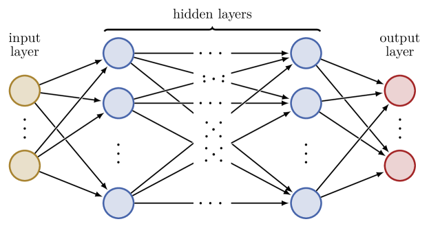
Figure 2. Illustration of a fully-connected feed-forward artificial neural network. The neurons are depicted as circles, and the connections represented by black arrows.

Neural network models can be understood as input/output systems that are governed by a collection of simple rules at each neuron of each layer. More precisely, we have an affine transformation of the corresponding input followed by the application of a scalar non-linear function, which is referred to as activation function. It is applied component-wise, see [Pin99, GBC16] for more details. Popular choices of the activation function include the hyperbolic tangent, the sigmoid function or rectified linear unit. The a priori unknown coefficients of the affine transformations correspond to the trainable parameters of the network. Formally, an ANN of depth $D>0$ having layers with widths $\{N_{k}\}_{k=0}^{D}$ is characterized by the sequence

$${\boldsymbol{\operatorname{\theta}}}:=\{({\boldsymbol{\operatorname{W}}}_{k},{\boldsymbol{\operatorname{b}}}_{k})\}_{k=1}^{D},$$

where ${\boldsymbol{\operatorname{W}}}_{k}\in{\mathbb{R}}^{N_{k}\times N_{k-1}}$ and ${\boldsymbol{\operatorname{b}}}_{k}\in{\mathbb{R}}^{N_{k}}$ constitute the above-mentioned trainable parameters associated to the $k$-th layer. They are called weight matrix and bias vector, respectively. The dimension of the parameter space containing ${\boldsymbol{\operatorname{\theta}}}$, which we denote by $\Theta$, amounts to $N_{\Theta}:=\sum_{k=1}^{D}N_{k}(N_{k-1}+1)$.

Next, we introduce the realization function for the type of ANNs considered in this work.

Definition 3.1 (Realization and network function).

Let ${\boldsymbol{\operatorname{\theta}}}:=\{({\boldsymbol{\operatorname{W}}}_{k},{\boldsymbol{\operatorname{b}}}_{k})\}_{k=1}^{D}$, which defines an ANN of depth $D>0$ and widths $\{N_{k}\}_{k=0}^{D}$. Moreover, let ${\boldsymbol{x}}\in{\mathbb{R}}^{N_{0}}$ denote an input of the ANN. The realization function $\operatorname{\boldsymbol{\mathcal{N}}}:{\mathbb{R}}^{N_{\Theta}}\to V_{\boldsymbol{\operatorname{\theta}}}$ yields a network function $v_{\boldsymbol{\operatorname{\theta}}}:=\operatorname{\boldsymbol{\mathcal{N}}({\boldsymbol{\operatorname{\theta}}})}$ mapping the input ${\boldsymbol{x}}$ to an output $v_{{\boldsymbol{\operatorname{\theta}}}}({\boldsymbol{x}})\in{\mathbb{R}}^{N_{D}}$ such that

$$v_{{\boldsymbol{\operatorname{\theta}}}}({\boldsymbol{x}}):=\operatorname{\boldsymbol{\mathcal{N}}({\boldsymbol{\operatorname{\theta}}})}({\boldsymbol{x}})=\mathcal{N}^{(D)}\circ\mathcal{N}^{(D-1)}\circ\dots\circ\mathcal{N}^{(1)}\circ\mathcal{N}^{(0)}({\boldsymbol{x}}),$$

where the realization functions of the different layers, denoted by $\mathcal{N}^{(\cdot)}$, are defined as

$$x_{0} =\mathcal{N}^{(0)}({\boldsymbol{x}})={\boldsymbol{x}},$$

$$x_{k} =\mathcal{N}^{(k)}({\boldsymbol{x}}_{k-1})=\sigma({\boldsymbol{\operatorname{W}}}_{k}{\boldsymbol{x}}_{k-1}+{\boldsymbol{\operatorname{b}}}_{k}),\qquad k=1,\dots,D-1,$$

$$v_{{\boldsymbol{\operatorname{\theta}}}}({\boldsymbol{x}}) =\mathcal{N}^{(D)}({\boldsymbol{x}}_{D-1})={\boldsymbol{\operatorname{W}}}_{D}{\boldsymbol{x}}_{D-1}+{\boldsymbol{\operatorname{b}}}_{D}.$$

Here, $\sigma:{\mathbb{R}}\to I\subset{\mathbb{R}}$ is a possibly non-linear activation function and $V_{\boldsymbol{\operatorname{\theta}}}\subset H^{1}(\Omega)$ denotes the space spanned by all possible network realizations.

3.2. Training

In machine learning terminology, the iterative optimization process of determining the unknown parameters ${\boldsymbol{\operatorname{\theta}}}$ is called training or learning. This generally involves a gradient descent method, which requires computing the gradient with respect to the trainable parameters at each step. The optimization process is achieved through backpropagation, which is a specific instance of the reverse mode of automatic differentiation [RHW86, Gri03, BPRS18]. Common optimizers such as the adaptive moment estimation (Adam), see [KB15], are based on a stochastic gradient descent method, see [BCN18]. Note that quasi-Newton methods, such as the limited-memory Broyden–Fletcher–Goldfarb–Shanno algorithm are also popular in the machine learning community [ZBLN97]. In the context of deep learning, second-order methods are mostly used a posteriori, after a gradient descent method for the sake of fine-tuning [GBC16]. Here, we only consider the Adam optimizer.

Taking into account the multiplicative nature of the network function from Definition 3.1, the backpropagated gradients may become excessively large or small. These pathologies are referred to as gradient exploding and gradient vanishing, respectively. This can be circumvented or at least reduced by a proper initialization of the trainable parameters ${\boldsymbol{\operatorname{\theta}}}$ together with a suitable activation function. In this work, we consider $\sigma:=\tanh\colon{\mathbb{R}}\to I:=(-1,1)$ as activation function, which is a non-linear, bounded, and smooth function. Note that for some applications, using $\tanh(\alpha_{k}x)$, $k=1,\dots,D-1$, with trainable coefficients $\alpha_{k}$ might be more robust and avoids a saturation of the gradient more effectively. Moreover, we opt for a Xavier/Glorot normal initialization. It helps to prevent gradients from exploding or vanishing by drawing the initial values of the parameters in the network from a normal distribution with zero mean and a variance that depends on the width of the network, namely, $\frac{2}{N_{k}+N_{k-1}}$, for all $k=1,\dots,D$. For more details, we refer to [GB10].

3.3. Loss function and practical realization

The final building block is to specify the optimization strategy, which is problem-dependent. When training neural networks, the goal is typically to find the set of parameters ${\boldsymbol{\operatorname{\theta}}}$ that minimizes an empirical loss function. For classical deep learning applications, especially regression tasks, a loss function is a differentiable function with respect to ${\boldsymbol{\operatorname{\theta}}}$, which is bounded from below. It measures the error between the actual network output $v_{{\boldsymbol{\operatorname{\theta}}}}({\boldsymbol{x}})$ and the targeted outcome that usually corresponds to known data or labels. Common loss functions of this type include the mean absolute error and mean squared error, also known as $L_{1}$ and $L_{2}$ loss functions, respectively. Recently, the development of automatic differentiation has opened the door to a plethora of neural-based solvers, in particular the so called physics-informed neural networks (PINNs), where in addition to possible data the governing “physical” model is incorporated in the loss function [RPK19]. Hence, boundary value problems can be approximated directly using neural network models as ansatz function. For more details and applications of PINNs, see [ZMM⁺21] and the references therein. For a mathematical justification, we refer e.g., to [SDK20, MM21].

Remark 3.2.

MLPs have the so-called universal approximation property, which implies (roughly speaking) that any continuous function can be approximated arbitrarily close by some neural network, provided the considered non-linear activation function fulfills certain properties regarding monotonicity, smoothness, and boundedness, see e.g., [Cyb89, HSW89]. This result motivated the use of neural networks as function approximators for solving differential equations prior to PINNs, as for instance in [LK90, LLF98].

In contrast to classical PINNs, our loss function is based on the constrained minimization problem (11) associated to the localized correction operator in (10). Such an ansatz is known as Deep Ritz method [EY18]. Note that in our case, no further data is needed for the training procedure except for a set of parametrized coefficients. We aim to replace $v\in H_{0}^{1}(\mathsf{N}^{\ell}(K))$ in (11) by a suitable network function with straightforward adaptations. First, to take into account the localization procedure, the output of the neural network should be transformed as follows to satisfy the homogeneous Dirichlet boundary condition on the considered patch.

Definition 3.3 (Localization of the network function).

Let the realization function $\operatorname{\boldsymbol{\mathcal{N}}}$ define an ANN with fixed architecture according to Definition 3.1, and let $v_{\boldsymbol{\operatorname{\theta}}}:=\operatorname{\boldsymbol{\mathcal{N}}({\boldsymbol{\operatorname{\theta}}})}\in V_{\boldsymbol{\operatorname{\theta}}}\subset H^{1}(\Omega)$ denote the resulting network function. For $\Omega^{\ell}\subset\Omega\subseteq{\mathbb{R}}^{d}$, $d\geq 1$, and $x\in\Omega$, a localized network function $v_{{\boldsymbol{\operatorname{\theta}}}}^{\ell}\in V_{\boldsymbol{\operatorname{\theta}}}(\Omega^{\ell})$ is understood as

$$v_{{\boldsymbol{\operatorname{\theta}}}}^{\ell}(x)=\begin{cases}g(v_{\boldsymbol{\operatorname{\theta}}}(x))&\text{ for }x\in\Omega^{\ell},\\ 0&\text{ otherwise},\end{cases}$$

where $g:{\mathbb{R}}^{N_{D}}\to{\mathbb{R}}^{N_{D}}$ is a smooth function that vanishes on $\partial\Omega^{\ell}$ and is non-zero in $\Omega^{\ell}$. In particular, for rectangular patches $\Omega^{\ell}:=(0,a)\times(0,b)$, $a,b>0$, and $x:=(x_{1},x_{2})^{\top}\in{\mathbb{R}}^{2}$, the considered function $g$ is chosen as

$$g(v_{\boldsymbol{\operatorname{\theta}}}(x))=\kappa x_{1}x_{2}(a-x_{1})(x_{2}-b)v_{\boldsymbol{\operatorname{\theta}}}(x),$$

where $\kappa>0$ is a scaling coefficient that is chosen depending on the problem. Note that in practice only $x\in\overline{\Omega^{\ell}}$ are taken into account during training. That is, we interpret $V_{\boldsymbol{\operatorname{\theta}}}(\Omega^{\ell})$ as a subspace of $H^{1}_{0}(\Omega^{\ell})$.

Without loss of generality, let us assume that the considered inputs of the ANN have the form ${\boldsymbol{x}}:=(x,{\boldsymbol{p}})$, where $x\in\Omega$ denotes the spatial coordinates and ${\boldsymbol{p}}\in{\mathbb{R}}^{N_{p}}$, $N_{p}\geq 0$, refers to a possible additional parametrization vector for the coefficient function $a:\Omega\times{\mathbb{R}}^{N_{p}}\to{\mathbb{R}}$, cf. Section 2.3.

Remark 3.4.

Considering inputs of the form ${\boldsymbol{x}}:=(x,{\boldsymbol{p}})$ allows us to clearly separate the spatial component from the parametrization, which constitutes the variable of interest in the context of generalization.

As a next step, we define the required loss functions to minimize the integral and penalize the constraint condition in (11), respectively. Afterwards, we introduce the fully discrete setting (including quadrature) that is used for computational purposes.

Definition 3.5 (Loss functions).

Let $\ell\geq 1$ and a basis function $\Lambda_{j}$ of $V_{H}$ and $T\in\mathcal{T}_{H}$ such that $T\cap\operatorname{supp}(\Lambda_{j})\neq\emptyset$ be given. Further, $v_{{\boldsymbol{\operatorname{\theta}}},j}^{\ell,T}\in V_{\boldsymbol{\operatorname{\theta}}}(\mathsf{N}^{\ell}(T))$ denotes a localized network function as defined in Definition 3.3 with $\Omega^{\ell}=\mathsf{N}^{\ell}(T)$. Given the parametrization vector ${\boldsymbol{p}}$, we define the energy loss function $\mathcal{L}_{\mathrm{energy}}\colon V_{\boldsymbol{\operatorname{\theta}}}(\mathsf{N}^{\ell}(T))\to{\mathbb{R}}$ by

(16) $$\mathcal{L}_{\mathrm{energy}}(v_{{\boldsymbol{\operatorname{\theta}}},j}^{\ell,T})=\frac{1}{2}\int_{\mathsf{N}^{\ell}(T)}a(x,{\boldsymbol{p}})\nabla v_{{\boldsymbol{\operatorname{\theta}}},j}^{\ell,T}(x,{\boldsymbol{p}})\cdot\nabla v_{{\boldsymbol{\operatorname{\theta}}},j}^{\ell,T}(x,{\boldsymbol{p}})\,\mathrm{d}x-\int_{T}a(x,{\boldsymbol{p}})\nabla\Lambda_{j}(x)\cdot\nabla v_{{\boldsymbol{\operatorname{\theta}}},j}^{\ell,T}(x,{\boldsymbol{p}})\,\mathrm{d}x,$$

and a loss function associated to the interpolation condition $\mathcal{L}_{\mathrm{interp}}\colon V_{\boldsymbol{\operatorname{\theta}}}(\mathsf{N}^{\ell}(T))\to{\mathbb{R}}_{\geq 0}$ by

(17) $$\mathcal{L}_{\mathrm{interp}}(v_{{\boldsymbol{\operatorname{\theta}}},j}^{\ell,T})=\int_{\mathsf{N}^{\ell}(T)}|\mathcal{I}_{H}v_{{\boldsymbol{\operatorname{\theta}}},j}^{\ell,T}(x,{\boldsymbol{p}})|^{2}\,\mathrm{d}x.$$

with the quasi-interpolation operator $\mathcal{I}_{H}:L^{2}(\Omega)\to V_{H}$ defined in (7). The total loss function of the neural correction problem is then computed as a linear combination of $\mathcal{L}_{\mathrm{energy}}$ and $\mathcal{L}_{\mathrm{interp}}$.

To ensure that the minimization problem actually has a minimizer, it needs to be bounded from below as proved in the following lemma.

Lemma 3.6.

The energy loss function (16) is bounded from below.

Proof.

The loss function in (16) for any $v\in H^{1}_{0}(\mathsf{N}^{\ell}(T))$ reads

$$\mathcal{L}_{\mathrm{energy}}(v)=\frac{1}{2}\mathfrak{A}|_{\mathsf{N}^{\ell}(T)}(v,v)-\mathfrak{A}|_{T}(\Lambda_{j},v).$$

The second term can be estimated by the Cauchy–Schwarz and Young’s inequality,

$$\mathfrak{A}|_{T}(\Lambda_{j},v)\leq\tfrac{1}{2}\|a^{1/2}\nabla\Lambda_{j}\|_{L^{2}(T)}^{2}+\tfrac{1}{2}\|a^{1/2}\nabla v\|_{L^{2}(T)}^{2}=\tfrac{1}{2}\mathfrak{A}|_{T}(\Lambda_{j},\Lambda_{j})+\tfrac{1}{2}\mathfrak{A}|_{T}(v,v).$$

Therefore, we obtain

$$\mathcal{L}_{\mathrm{energy}}(v) =\tfrac{1}{2}\mathfrak{A}|_{\mathsf{N}^{\ell}(T)}(v,v)-\mathfrak{A}|_{T}(\Lambda_{j},v)\geq\tfrac{1}{2}\mathfrak{A}|_{\mathsf{N}^{\ell}(T)}(v,v)-\tfrac{1}{2}\mathfrak{A}|_{T}(\Lambda_{j},\Lambda_{j})-\tfrac{1}{2}\mathfrak{A}|_{T}(v,v)$$

$$\geq-\tfrac{1}{2}\mathfrak{A}|_{T}(\Lambda_{j},\Lambda_{j}),$$

where the last inequality follows from $\mathfrak{A}|_{\mathsf{N}^{\ell}(T)}(v,v)\geq\mathfrak{A}|_{T}(v,v)$. ∎

The computation of the integrals in (16) can be performed using numerical quadrature rules. In this case, the quadrature points would constitute the spatial component of the input. As stated in Remark 3.4, we are rather interested in the prediction of correction functions for arbitrary coefficients $a$ in some given spectrum, which is determined by a set of distinct parametrization vectors collected in ${{\boldsymbol{p}}}:=\{{\boldsymbol{p}}_{k}\}_{j=1}^{N_{\mathrm{s}}}$, $N_{\mathrm{s}}\geq 1$. We consider a simple quadrature rule based on a classical space discretization of (16) using a finite element ansatz. More precisely, we consider a finite element space $V_{h}$ defined analogously to (5) with mesh size $h<\varepsilon$ that resolves the fine scale. Further, we consider the underlying mesh $\mathcal{T}_{h}$ to be a refinement of $\mathcal{T}_{H}$, such that $V_{H}\subset V_{h}$. We denote with $\{\lambda_{j}\}_{j=1}^{N_{h}}$ the nodal basis of $V_{h}$, where $N_{h}=\dim V_{h}$. For convenience and as a preliminary step, we first consider global correction problems on $\Omega$, i.e., with a patch big enough to contain the whole domain ($\ell=\infty$). Based on the fine mesh $\mathcal{T}_{h}$, the network function is approximated for each sample ${\boldsymbol{p}}_{k}\in{\mathbb{R}}^{N_{p}}$ by

(18) $$v_{{\boldsymbol{\operatorname{\theta}}},j}^{\infty,T}(x,{\boldsymbol{p}}_{k})=\sum_{j=1}^{N_{h}}\alpha_{j}(z_{j},{\boldsymbol{p}}_{k})\lambda_{j}(x),\quad x\in\Omega,$$

where ${\boldsymbol{z}}:=\{z_{j}\}_{j=1}^{N_{h}}$, $z_{j}\in{\mathbb{R}}^{d}$ contains the nodes of the fine mesh $\mathcal{T}_{h}$. Hence, the output of the neural network reduces to $\boldsymbol{\alpha}({\boldsymbol{z}},{\boldsymbol{p}}_{k}):=(\alpha_{1}(z_{1},{\boldsymbol{p}}_{k}),\dots,\alpha_{N_{h}}(z_{N_{h}},{\boldsymbol{p}}_{k}))$. For notational simplicity, we omit the specification of the spatial component ${\boldsymbol{z}}$ in the argument of ${\boldsymbol{\alpha}}$ and write $\boldsymbol{\alpha}_{{\boldsymbol{p}}_{k}}$ instead of $\boldsymbol{\alpha}({\boldsymbol{z}},{\boldsymbol{p}}_{k})$. Altogether, the input dataset for the ANN is defined by $\widecheck{{\boldsymbol{x}}}:={\boldsymbol{z}}\times{{\boldsymbol{p}}}\in{\mathbb{R}}^{N_{0}\times N_{h}N_{\mathrm{s}}}$ with input dimension $N_{0}=d+N_{p}$ and $N_{h}N_{\mathrm{s}}$ training samples. The resulting output is denoted by ${\boldsymbol{\alpha}}(\widecheck{{\boldsymbol{x}}}):=\boldsymbol{\operatorname{\alpha}}_{\boldsymbol{p}}:=(\boldsymbol{\alpha}_{{\boldsymbol{p}}_{1}},\dots,\boldsymbol{\alpha}_{{\boldsymbol{p}}_{N_{\mathrm{s}}}})^{\top}\in{\mathbb{R}}^{N_{h}N_{\mathrm{s}}}$.

To approximate (16), let first for a given $j\in\{1,\ldots,N_{H}\}$ the vector $\boldsymbol{\gamma}:=(\gamma_{1},\ldots,\gamma_{N_{h}})^{\top}\in{\mathbb{R}}^{N_{h}}$ be such that

$$\Lambda_{j}(x)=\sum_{j=1}^{N_{h}}\gamma_{i}\lambda_{i}(x)$$

represents the coarse basis function $\Lambda_{j}\in V_{H}$ via the fine basis functions of $V_{h}$. Next, we define $\boldsymbol{\Lambda}_{j}:=\mathbf{1}\otimes\boldsymbol{\gamma}$ with $\textbf{1}=(1,\ldots,1)^{\top}\in{\mathbb{R}}^{N_{\mathrm{s}}}$ as the $N_{\mathrm{s}}$-times repeated vector $\boldsymbol{\gamma}$ (using the Kronecker product). Further, $\boldsymbol{S}^{h}_{\boldsymbol{p}}:=\operatorname{diag}(S_{h}({\boldsymbol{p}}_{1}),\ldots,S_{h}({\boldsymbol{p}}_{N_{\mathrm{s}}}))$ denotes the block-diagonal matrix with $N_{\mathrm{s}}$ blocks, whose elements $S_{h}({\boldsymbol{p}}_{k})\in{\mathbb{R}}^{N_{h}\times N_{h}}$ are the stiffness matrices with respect to the fine mesh $\mathcal{T}_{h}$ and the parameter sample ${\boldsymbol{p}}_{k}$. We then obtain the following approximation of (16)

(19) $$\widehat{\mathcal{L}}_{\mathrm{energy}}(\boldsymbol{\operatorname{\alpha}}_{\boldsymbol{p}})=\frac{1}{2}\boldsymbol{\operatorname{\alpha}}_{\boldsymbol{p}}^{\top}\boldsymbol{S}_{\boldsymbol{p}}^{h}\boldsymbol{\operatorname{\alpha}}_{\boldsymbol{p}}-\boldsymbol{\Lambda}_{j}^{\top}\boldsymbol{S}_{\boldsymbol{p}}^{h}\boldsymbol{\operatorname{\alpha}}_{\boldsymbol{p}}.$$

Note that using the approximated loss function (19) in the training procedure is a significant simplification compared to the original problem by avoiding the online computation of gradients and reducing the number of sensors, i.e., points where the solution should be learned, to the dimension of the fine mesh $V_{h}$ for each ${\boldsymbol{p}}_{k}$.

As an approximation of the second term (17), we choose the $L_{2}$-loss evaluated at the same input $\widecheck{{\boldsymbol{x}}}$. Formally, given the matrix-version of the quasi-interpolation operator ${\mathcal{I}_{H}}$ for functions in $V_{h}$ denoted by $I_{H}\colon{\mathbb{R}}^{N_{h}}\to{\mathbb{R}}^{N_{H}}$, we obtain

(20) $$\widehat{\mathcal{L}}_{\mathrm{interp}}(\boldsymbol{\operatorname{\alpha}}_{\boldsymbol{p}})=\frac{1}{N_{\mathrm{s}}N_{H}}\|\boldsymbol{I}_{H}\boldsymbol{\operatorname{\alpha}}_{\boldsymbol{p}}\|^{2}_{2},$$

where $\boldsymbol{I}_{H}=\operatorname{diag}(I_{H},\ldots,I_{H})$ is the block-diagonal matrix with $N_{\mathrm{s}}$ blocks containing $I_{H}$.

Next, to define the total loss function, a weighted sum of the loss terms (19) and (20) is considered, as indicated in Definition 3.5. However, the choice of the weights is detrimental for the success of the training process. Indeed, depending on the problem, each term of the loss function may produce gradients of different orders of magnitudes during back-propagation with a gradient-based optimizer. This leads to training stagnation and often to wrong predictions due to an imbalance of the corresponding convergence rates. In the context of PINNs, this pathology has already been observed and studied in several works, giving rise to different approaches aiming at correcting this discrepancy. We refer to [WYP22] for a theoretical insight on this issue, where a possible approach to adaptively calibrate the convergence rates of the different loss terms has been proposed. In this work, we opt for a different approach, following the idea of self-adaptive PINNs (SA-PINNs) introduced in [MBN23]. As the name suggests, the determination of suitable weights is left to the ANN. In our case we associate a weight to each of the training points of the term (20). The self-adaptation in SA-PINNs consists in increasing the weights that are associated to training points, where the loss function is increasing. Together with the original minimization problem with respect to the trainable parameters of the network, this leads to a saddle-point problem. In practice, the incorporation of the self-adaptive weights is achieved through a mask function that is assumed to be non-negative, differentiable, and strictly increasing, see [MBN23]. In our case, we extend (20) by positive self-adaptive weights ${\boldsymbol{\operatorname{\mu}}}:=(\mu_{1},\dots,\mu_{N_{\mathrm{s}}N_{H}})\in{\mathbb{R}}_{>0}^{N_{\mathrm{s}}N_{H}}$ and write

(21) $$\widehat{\mathcal{L}}_{\mathrm{interp}}(\boldsymbol{\operatorname{\alpha}}_{\boldsymbol{p}},{\boldsymbol{\operatorname{\mu}}})=\frac{1}{N_{\mathrm{s}}N_{H}}\|{\boldsymbol{\operatorname{\mu}}}\odot\boldsymbol{I}_{H}\boldsymbol{\operatorname{\alpha}}_{\boldsymbol{p}}\|^{2}_{2},$$

where the operation $\odot$ is understood as a component-wise multiplication. Note that it is important that ${\boldsymbol{\operatorname{\mu}}}$ only contains positive entries, which can be guaranteed using a suitable initialization. In this work, the self-adaptive weights $\mu_{j}$ are initialized from a random uniform distribution on $(0,1)$. With this, the self-adaptive total loss function $\widehat{\mathcal{L}}:{\mathbb{R}}^{N_{\mathrm{s}}N_{h}}\times{\mathbb{R}}^{N_{\mathrm{s}}N_{H}}\to{\mathbb{R}}$ is defined by

(22) $$\widehat{\mathcal{L}}(\boldsymbol{\operatorname{\alpha}}_{\boldsymbol{p}},{\boldsymbol{\operatorname{\mu}}})=\widehat{\mathcal{L}}_{\mathrm{energy}}(\boldsymbol{\operatorname{\alpha}}_{\boldsymbol{p}})+\widehat{\mathcal{L}}_{\mathrm{interp}}(\boldsymbol{\operatorname{\alpha}}_{\boldsymbol{p}},{\boldsymbol{\operatorname{\mu}}})$$

with $\widehat{\mathcal{L}}_{\mathrm{energy}}(\boldsymbol{\operatorname{\alpha}}_{\boldsymbol{p}})$ and $\widehat{\mathcal{L}}_{\mathrm{interp}}(\boldsymbol{\operatorname{\alpha}}_{\boldsymbol{p}},{\boldsymbol{\operatorname{\mu}}})$ as given in (19) and (21), respectively.

3.4. Localization and training

As a penultimate step, and similarly to Definition 3.3, we address the localization procedure for the discrete setting and the adopted notations. Given a localization parameter $\ell\geq 1$, we denote the localized coefficients corresponding to $v_{{\boldsymbol{\operatorname{\theta}}},j}^{\ell,T}$ by ${\boldsymbol{\operatorname{\alpha}}_{\boldsymbol{p}}^{\ell}}$. The subset ${\boldsymbol{\operatorname{\alpha}}_{\boldsymbol{p}}^{\ell}}\subseteq\boldsymbol{\operatorname{\alpha}}_{\boldsymbol{p}}$ reduces to all coefficients that are associated to

$${\boldsymbol{z}}^{\ell}:=\{z_{k}\}_{k=1}^{N_{h}^{\ell}}$$

containing all $z_{k}\in\mathsf{N}^{\ell}(T)$, where $N_{h}^{\ell}=\dim V_{h}(\mathsf{N}^{\ell}(T))\leq N_{h}$. Note that we implicitly assume for the moment that the first $N_{h}^{\ell}$ nodes of the whole mesh lie in the patch $\mathsf{N}^{\ell}(T)$ to avoid a re-numbering. The coefficients associated to $z_{k}\notin\mathsf{N}^{\ell}(T)$ are fixed to zero and thus excluded from the training process. Correspondingly, we refer to the localized counterparts of $\boldsymbol{S}_{\boldsymbol{p}}^{h}$, $\boldsymbol{\Lambda}_{j}$, and $\boldsymbol{I}_{H}$ restricted to $\mathsf{N}^{\ell}(T)$ by $\boldsymbol{S}_{\boldsymbol{p}}^{h,\ell}$, $\boldsymbol{\Lambda}_{j}^{\ell}$, and $\boldsymbol{I}^{\ell}_{H}$, respectively.

Finally, we formulate the localized neural-based correction problem.

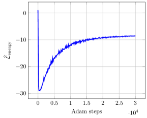
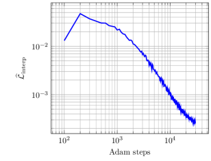
Figure 3. The respective parts of the total loss function for the correction of the basis function associated to node $(0.5,0.5)$ in Example 1. On the left the energy functional loss $\widehat{\mathcal{L}}_{\mathrm{energy}}$ and on the right the interpolation loss $\widehat{\mathcal{L}}_{\mathrm{interp}}$ in a log-log-plot is shown.

Problem 3.7 (Training procedure).

Let $\ell\geq 1$ and a basis function $\Lambda_{j}$ of $V_{H}$ and $T\in\mathcal{T}_{H}$ such that $T\cap\operatorname{supp}(\Lambda_{j})\neq\emptyset$ be given. Further, let $v_{{\boldsymbol{\operatorname{\theta}}},j}^{\ell,T}:=\operatorname{\boldsymbol{\mathcal{N}}({\boldsymbol{\operatorname{\theta}}})}$ be a network function defining an ANN with trainable network parameters ${\boldsymbol{\operatorname{\theta}}}\in{\mathbb{R}}^{N_{\Theta}}$ according to Definition 3.1. Using the approximation (18), the input dataset reads $\widecheck{{\boldsymbol{x}}}:={\boldsymbol{z}}^{\ell}\times{{\boldsymbol{p}}}\in{\mathbb{R}}^{(d+N_{p})\times n}$ with $n=N^{\ell}_{h}N_{\mathrm{s}}$ and the localized output ${\boldsymbol{\operatorname{\alpha}}_{\boldsymbol{p}}^{\ell}}$ has the dimension $n$. Then, the training procedure for the self-adaptive neural-based correction problem reads: find ${\boldsymbol{\operatorname{\alpha}}_{\boldsymbol{p}}^{\ell}}^{\star}\in{\mathbb{R}}^{n}$ such that

(23) $${\boldsymbol{\operatorname{\alpha}}_{\boldsymbol{p}}^{\ell}}^{\star}=\adjustlimits{\operatorname*{argmin}}_{{\boldsymbol{\operatorname{\alpha}}_{\boldsymbol{p}}^{\ell}}\in{\mathbb{R}}^{n}}{\max}_{{\boldsymbol{\operatorname{\mu}}}^{\ell}\in{\mathbb{R}}^{N}}\widehat{\mathcal{L}}({\boldsymbol{\operatorname{\alpha}}_{\boldsymbol{p}}^{\ell}},{\boldsymbol{\operatorname{\mu}}}^{\ell}),\qquad\widehat{\mathcal{L}}({\boldsymbol{\operatorname{\alpha}}_{\boldsymbol{p}}^{\ell}},{\boldsymbol{\operatorname{\mu}}}^{\ell})=\widehat{\mathcal{L}}_{\mathrm{energy}}({\boldsymbol{\operatorname{\alpha}}_{\boldsymbol{p}}^{\ell}})+\widehat{\mathcal{L}}_{\mathrm{interp}}({\boldsymbol{\operatorname{\alpha}}_{\boldsymbol{p}}^{\ell}},{\boldsymbol{\operatorname{\mu}}}^{\ell}),$$

where $N_{H}^{\ell}=\dim V_{H}(\mathsf{N}^{\ell}(T))$, $N=N^{\ell}_{H}N_{\mathrm{s}}$, and

(24) $$\widehat{\mathcal{L}}_{\mathrm{interp}}({\boldsymbol{\operatorname{\alpha}}_{\boldsymbol{p}}^{\ell}},{\boldsymbol{\operatorname{\mu}}}^{\ell})=\frac{1}{N}\|{\boldsymbol{\operatorname{\mu}}}^{\ell}\odot\boldsymbol{I}^{\ell}_{H}{\boldsymbol{\operatorname{\alpha}}_{\boldsymbol{p}}^{\ell}}\|^{2}_{2}$$

with the self-adaptive weight vector ${\boldsymbol{\operatorname{\mu}}}^{\ell}\in{\mathbb{R}}^{N}$ and

$$\widehat{\mathcal{L}}_{\mathrm{energy}}({\boldsymbol{\operatorname{\alpha}}_{\boldsymbol{p}}^{\ell}})=\frac{1}{2}\big{(}{\boldsymbol{\operatorname{\alpha}}_{\boldsymbol{p}}^{\ell}}\big{)}^{\top}\boldsymbol{S}_{\boldsymbol{p}}^{h,\ell}{\boldsymbol{\operatorname{\alpha}}_{\boldsymbol{p}}^{\ell}}-\big{(}\boldsymbol{\Lambda}_{j}^{\ell}\big{)}^{\top}\boldsymbol{S}_{\boldsymbol{p}}^{h,\ell}{\boldsymbol{\operatorname{\alpha}}_{\boldsymbol{p}}^{\ell}}.$$

Given some ${\boldsymbol{x}}:=(x,{\boldsymbol{p}})\in\Omega\times{\mathbb{R}}^{N_{p}}$, the localized correction $v_{{\boldsymbol{\operatorname{\theta}}},j}^{\ell,T}({\boldsymbol{x}})$ as a function is realized as in (18).

Remark 3.8.

Note that due the monotonicity of the considered activation function $\tanh$ and by construction of the realization function (see Definition 3.1), the optimization of (23) is equivalent to finding ${\boldsymbol{\operatorname{\theta}}}^{\star}\in{\mathbb{R}}^{N_{\Theta}}$ such that

(25) $${\boldsymbol{\operatorname{\theta}}}^{\star}=\adjustlimits{\operatorname*{argmin}}_{{\boldsymbol{\operatorname{\theta}}}\in{\mathbb{R}}^{N_{\Theta}}}{\max}_{{\boldsymbol{\operatorname{\mu}}}^{\ell}\in{\mathbb{R}}^{N}}\widehat{\mathcal{L}}({\boldsymbol{\operatorname{\alpha}}_{\boldsymbol{p}}^{\ell}},{\boldsymbol{\operatorname{\mu}}}^{\ell}).$$

In other words, the localized correction function that minimizes (23) corresponds to the output of the network function induced by ${\boldsymbol{\operatorname{\theta}}}^{\star}$.

In a post-processing step, i.e., after training the ANN by solving (23) (or equivalently (25)), we compute the corrected multiscale basis $\{\widehat{\Lambda}_{j}^{\ell}\}_{j=1}^{N_{H}}$ that spans the modified multiscale space $\widehat{V}_{H}^{\ell}$. That is, each $\widehat{\Lambda}_{j}^{\ell}$ is associated to the corresponding basis function $\Lambda_{j}$ of $V_{H}$ and related to the coefficient function $a\colon\Omega\times{\mathbb{R}}^{N_{p}}\to{\mathbb{R}}$ induced by ${\boldsymbol{p}}$. More precisely, it is obtained similarly to (12) by

(26) $$\big{(}\widehat{\Lambda}_{j}^{\ell}({\boldsymbol{p}})\big{)}(x)=\Lambda_{j}(x)-\sum_{T\in\mathcal{T}_{H}\colon\operatorname{supp}(\Lambda_{j})\cap T\neq\emptyset}v_{{\boldsymbol{\operatorname{\theta}}},j}^{\ell,T}(x,{\boldsymbol{p}}).$$

By computing/predicting the multiscale basis functions corresponding to all $\Lambda_{j}\in V_{H}$, $j=1,\dots,N_{H}$, solving equation (13) follows the lines of the classical LOD approach, cf. [MP20]. That is, for an elliptic model problem and given some parameter ${\boldsymbol{p}}$, we compute the Galerkin solution in the space $\widehat{V}_{H}^{\ell}$. This requires the computation of appropriate system matrices making use of the corrected basis functions. For time-dependent or uncertain problems, such matrices need to be updated based on the choice of ${\boldsymbol{p}}$ during simulations. To compute such matrices more efficiently, a Petrov–Galerkin variant of the LOD may be used, see also [EHMP19]. In the following section, we present numerical examples to illustrate the performance of the considered approach and its generalization capability.

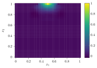
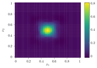
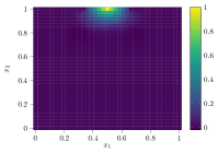
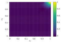
Figure 4. Illustrations of different corrected basis functions $\widetilde{\Lambda}_{j}^{\ell}$ for each possible patch configurations for $\ell=1$ in Example 1. The top row shows the classical LOD basis functions, while the bottom row depicts their learned analogs.

4. Numerical Examples

In order to apply our method to the parabolic equation (2), we consider the variational formulation (3) and discretize it in space and time. For the spatial discretization, we first employ for a given ${\boldsymbol{p}}$ the classical LOD space $\widetilde{V}_{H}^{\ell}$ as given in Definition 2.4 combined with a backward Euler method. The corresponding approximate solution in the $m$th time step is denoted by $\widetilde{u}_{H}^{m}$ and serves as a reference solution. Second, we compute an LOD-ANN space $\widehat{V}_{H}^{\ell}$ for the spatial approximation based on the derivations in Section 3, again based on a backward Euler method in time. The corresponding approximate solution in the $m$th time step is denoted by $\widehat{u}_{H}^{m}$. Note that the time step for both approaches is given by $\tau={T}/{M}$, where $M$ is the number of time steps. The error $\widehat{u}_{H}^{m}-u(t_{m})$ with the exact solution $u(t_{m})$ at time $t_{m}=m\tau$ scales like

(27) $$\|\nabla(\widehat{u}_{H}^{m}-u(t_{m}))\|_{L^{2}(\Omega)} \leq\|\nabla(\widehat{u}_{H}^{m}-\widetilde{u}_{H}^{m})\|_{L^{2}(\Omega)}+\|\nabla(\widetilde{u}_{H}^{m}-u(t_{m}))\|_{L^{2}(\Omega)}$$

$$\leq\|\nabla(\widehat{u}_{H}^{m}-\widetilde{u}_{H}^{m})\|_{L^{2}(\Omega)}+C_{\mathrm{LOD}}(\tau+H)+e_{\mathrm{disc}},$$

where $e_{\mathrm{disc}}$ is the fine-scale discretization error and $C_{\mathrm{LOD}}>0$ arises from classical LOD and backward Euler theory (see, e.g., [MP18, MP20]) and is independent of $\varepsilon$, $H$, and $h$.

Analogously, for the elliptic problem (13) we have

(28) $$\|\nabla(\widehat{u}_{H}-u)\|_{L^{2}(\Omega)}\leq\|\nabla(\widehat{u}_{H}-\widetilde{u}_{H})\|_{L^{2}(\Omega)}+C_{\mathrm{LOD}}H+e_{\mathrm{disc}},$$

where $C_{\mathrm{LOD}}$ is again independent of $\varepsilon$, $H$, and $h$.

First example

The first example is a proof of concept, where we only consider the elliptic setting (13) with $f\equiv 1$. We show that ANNs are capable of capturing the fine oscillations of the modified basis functions and the corresponding approximate solution behaves similarly as the original LOD method. Further, we observe that once a network is trained, it is able to produce accurate basis functions corresponding to coefficients that have not been seen during the training process. We note here that apart from the coefficients we have not used any data in the training process as the overall error already is sufficiently small. However, it is possible to speed up the training process and improve the accuracy using pre-computed LOD basis functions for a certain set of coefficients as data.

The set of coefficients used for training consists of $40$ piece-wise constant functions on a scale $\varepsilon=0.001$ with oscillations between $\alpha=0.1$ and $\beta=1$. We learn the corrections according to Problem 3.7 with $\ell=1$, $H=1/6$, and $h=1/36$. The model is set up as a fully connected ANN with width $128$, and depth $8$. We trained over $30.000$ epochs using the Adam optimizer with an exponential decay as learning rate schedule (initial learning rate $10^{-3}$ with decay rate of $0.9$ and $1000$ decay steps). The respective values of the loss function are depicted in Figure 3. We observe that the energy loss function is being minimized early on and once the adaptive weights ${\boldsymbol{\operatorname{\mu}}}$ are large enough, the corrections are adapted to fulfill the interpolation condition.

During the training process, we achieve a mean train error over the $40$ samples of $4.42\%$. The test set consists of $20$ distinct randomly generated coefficients with the same upper and lower bound as the train coefficients. The mean test error is $4.78\%$. In Figure 4 corrected basis functions of the LOD and LOD-ANN methods are shown for all possible patch configurations for $\ell=1$.

Further, in Figure 5 (left) we depict a coefficient of the test set, the corresponding LOD solution (middle), and the LOD-ANN solution (right). The error between the solutions is $4.1\%$. That is, the total error scales like $0.041+C_{\mathrm{LOD}}H+e_{\mathrm{disc}}\leq(1+C_{\mathrm{LOD}})H+e_{\mathrm{disc}}$ using the error representation (28).

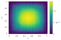
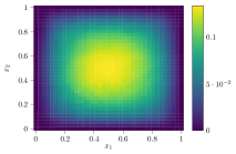
Figure 5. Coefficient of the test set (left) as well as the corresponding LOD solution (middle) and LOD-ANN solution (right) for Example 1.

Second example

For the second example, we consider the simplified model of [Ves22] in the context of battery simulations. It reads

(29) $$\rho\,\partial_{t}c_{\mathrm{p}}u-\operatorname{div}(\overline{\lambda}\nabla u)=f$$

with homogeneous boundary conditions, where $\overline{\lambda}$ denotes the heat conductivity and the density $\rho$ as well as the specific heat capacity $c_{\mathrm{p}}$ are assumed to be constant in time. The model is equivalent to (2) with $a={\overline{\lambda}}/{\rho c_{\mathrm{p}}}$ with a scaled right-hand side. The model is assumed to be partially homogenized, see also [Ves22]. The specific heat conductivity $\overline{\lambda}$ is portrayed in Figure 6 with the cathode collector (CC, green), the anode collector (AC, yellow) and the active material (AM, purple), subject to the material properties of Table 1 below.

	$\rho$	$c_{\mathrm{p}}$	$\lambda$
AC	8710.2	384.65	398.65
CC	2706.77	897.8	236.3
AM	2094.302	1010.119	$[1,10]$

Table 1. Material properties in Example 2

Note that for the AM we consider a range for the heat conductivity with unknown explicit value, which is in line with the uncertainty assumptions mentioned in Section 2.3. Specifically, we have no a priori knowledge on the coefficient in the offline phase prior to the simulations, such that we have to consider a whole range of possible approximation spaces as well.

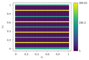
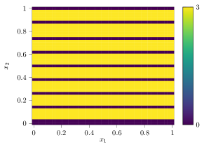
Figure 6. Coefficient for the partially homogenized heat conductivity (left), and the right-hand side function $f$ (right) for Example 2.

We set up the neural network analogously to the first example with the same depth and widths and use the Adam optimizer with the same learning rate. We train the model using six different parametrizations. In Figure 7, the comparison between an LOD basis function and the corresponding LOD-ANN basis function is shown. The computations are performed based on a coarse mesh with $H=1/8$, and we set $\ell=2$ and $h=1/40$. Here the material property for the AM is $\overline{\lambda}=5$ (which has not been considered during training) and the error of the depicted basis function is $6.1\%$.

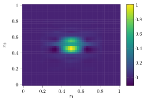
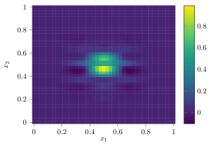
Figure 7. Visual comparison of an LOD basis function (left) and its LOD-ANN analog (right) for $\overline{\lambda}=5$ in the AM.

In Figure 8, we depict the solutions corresponding to the LOD and LOD-ANN method for different points in time. The initial condition is given by $u_{0}\equiv 0$ and the right-hand side $f$ is shown in Figure 6. The time step size is given by $\tau=0.6$ and the error at the final time $T=60$ seconds is $7.8\%$. Altogether, using equation (27), we obtain a total error of $0.078+C_{\mathrm{LOD}}(\tau+H)+e_{\mathrm{disc}}\leq C_{\mathrm{LOD}}\tau+(1+C_{\mathrm{LOD}})H+e_{\mathrm{disc}}$.

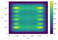
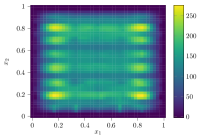
Figure 8. Solutions for the partially homogenized battery model. On the top the LOD solutions for times $t=0$, $t=30$ and $t=60$ seconds are shown, and on the bottom the solutions of the LOD-ANN method at the same times.

Note that the practical simulation of batteries is much more involved, and different boundary conditions as well as greater heterogeneities in the heat conductivity coefficient may be considered. In general, the active material is not homogeneous but strongly non-periodic and heterogeneous, which can again be effectively modeled considering a combinations of both examples.

5. Conclusions and Outlook

We have presented a numerical homogenization strategy based on the LOD method using a Deep Ritz approach for computing the corrections to leverage generalization properties of neural networks to, e.g., overcome the bottleneck of re-computations in the case of time-dependence or uncertainties in the PDE coefficient. This work is supposed to be a proof of concept regarding the replacement of the correction by a neural network-based ansatz function that is minimized with a constraint condition. In particular, it is trained based on an additional parametrization to eventually allow for quick computations of required corrections based on a given coefficient. We have presented two examples to illustrate the performance of the approach.

A straight-forward extensions is the amplification of the Deep Ritz method using different ANN architectures. A more technical modification would be a suitable addition of the localization parameter to the training parameters. Finally, a rigorous a posteriori analysis is still open.

References

- [AB05] G. Allaire and R. Brizzi. A multiscale finite element method for numerical homogenization. Multiscale Model. Simul., 4(3):790–812, 2005.
- [Abd16] A. Abdulle. Numerical homogenization methods for parabolic monotone problems. In Building bridges: connections and challenges in modern approaches to numerical partial differential equations, volume 114 of Lect. Notes Comput. Sci. Eng., pages 1–38. Springer, [Cham], 2016.
- [ACM+20] R. Altmann, E. Chung, R. Maier, D. Peterseim, and S.-M. Pun. Computational multiscale methods for linear heterogeneous poroelasticity. J. Comput. Math., 38(1):41–57, 2020.
- [AEEV12] A. Abdulle, W. E, B. Engquist, and E. Vanden-Eijnden. The heterogeneous multiscale method. Acta Numer., 21:1–87, 2012.
- [AH17] A. Abdulle and M. E. Huber. Numerical homogenization method for parabolic advection-diffusion multiscale problems with large compressible flows. Numer. Math., 136(3):603–649, 2017.
- [AHP21] R. Altmann, P. Henning, and D. Peterseim. Numerical homogenization beyond scale separation. Acta Numer., 30:1–86, 2021.
- [AP12] A. Abdulle and G. A. Pavliotis. Numerical methods for stochastic partial differential equations with multiple scales. J. Comput. Phys., 231(6):2482–2497, 2012.
- [AV12] A. Abdulle and G. Vilmart. Coupling heterogeneous multiscale FEM with Runge-Kutta methods for parabolic homogenization problems: a fully discrete spacetime analysis. Math. Models Methods Appl. Sci., 22(6):1250002, 40, 2012.
- [BCN18] L. Bottou, F. E. Curtis, and J. Nocedal. Optimization methods for large-scale machine learning. SIAM Rev., 60(2):223–311, 2018.
- [BL11] I. Babuska and R. Lipton. Optimal local approximation spaces for generalized finite element methods with application to multiscale problems. Multiscale Model. Simul., 9(1):373–406, 2011.
- [BPRS18] A. G. Baydin, B. A. Pearlmutter, A. A. Radul, and J. M. Siskind. Automatic differentiation in machine learning: a survey. J. Mach. Learn. Res., 18:1–43, 2018.
- [BS08] S. C. Brenner and L. R. Scott. The mathematical theory of finite element methods, volume 15 of Texts in Applied Mathematics. Springer, New York, third edition, 2008.
- [CELY18] E. T. Chung, Y. Efendiev, W. T. Leung, and S. Ye. Generalized multiscale finite element methods for space-time heterogeneous parabolic equations. Comput. Math. Appl., 76(2):419–437, 2018.
- [Cyb89] G. Cybenko. Approximation by superpositions of a sigmoidal function. Math. Control Signals Systems, 2(4):303–314, 1989.
- [EE03] W. E and B. Engquist. The heterogeneous multiscale methods. Commun. Math. Sci., 1(1):87–132, 2003.
- [EE05] W. E and B. Engquist. The heterogeneous multi-scale method for homogenization problems. In Multiscale methods in science and engineering, volume 44 of Lect. Notes Comput. Sci. Eng., pages 89–110. Springer, Berlin, Heidelberg, 2005.
- [EG17] A. Ern and J.-L. Guermond. Finite element quasi-interpolation and best approximation. ESAIM Math. Model. Numer. Anal., 51(4):1367–1385, 2017.
- [EGH13] Y. Efendiev, J. Galvis, and T. Y. Hou. Generalized multiscale finite element methods (GMsFEM). J. Comput. Phys., 251:116–135, 2013.
- [EHMP19] C. Engwer, P. Henning, A. Målqvist, and D. Peterseim. Efficient implementation of the localized orthogonal decomposition method. Comput. Methods Appl. Mech. Engrg., 350:123–153, 2019.
- [EV23] D. Eckhardt and B. Verfürth. Fully discrete heterogeneous multiscale method for parabolic problems with multiple spatial and temporal scales. BIT, 63(2):Paper No. 35, 26, 2023.
- [EY18] W. E and B. Yu. The deep Ritz method: a deep learning-based numerical algorithm for solving variational problems. Commun. Math. Stat., 6(1):1–12, 2018.
- [FGP21] J. Fischer, D. Gallistl, and D. Peterseim. A priori error analysis of a numerical stochastic homogenization method. SIAM J. Numer. Anal., 59(2):660–674, 2021.
- [GB10] X. Glorot and Y. Bengio. Understanding the difficulty of training deep feedforward neural networks. In Proceedings of the thirteenth international conference on artificial intelligence and statistics, pages 249–256. JMLR Workshop and Conference Proceedings, 2010.
- [GBC16] I. Goodfellow, Y. Bengio, and A. Courville. Deep learning. MIT press, 2016.
- [GP19] D. Gallistl and D. Peterseim. Numerical stochastic homogenization by quasilocal effective diffusion tensors. Commun. Math. Sci., 17(3):637–651, 2019.
- [Gri03] A. Griewank. A mathematical view of automatic differentiation. Acta Numer., 12:321–398, 2003.
- [HFMQ98] T. J. R. Hughes, G. R. Feijóo, L. Mazzei, and J.-B. Quincy. The variational multiscale method – a paradigm for computational mechanics. Comput. Methods Appl. Mech. Engrg., 166(1-2):3–24, 1998.
- [HKM20] F. Hellman, T. Keil, and A. Målqvist. Numerical upscaling of perturbed diffusion problems. SIAM J. Sci. Comput., 42(4):A2014–A2036, 2020.
- [HM19] F. Hellman and A. Målqvist. Numerical homogenization of elliptic PDEs with similar coefficients. Multiscale Model. Simul., 17(2):650–674, 2019.
- [HMP24] M. Hauck, H. Mohr, and D. Peterseim. A simple collocation-type approach to numerical stochastic homogenization. ArXiv Preprint, 2404.01732, 2024.
- [HP13] P. Henning and D. Peterseim. Oversampling for the multiscale finite element method. Multiscale Model. Simul., 11(4):1149–1175, 2013.
- [HSW89] K. Hornik, M. Stinchcombe, and H. White. Multilayer feedforward networks are universal approximators. Neural Netw., 2(5):359–366, 1989.
- [Hug95] T. J. R. Hughes. Multiscale phenomena: Green’s functions, the Dirichlet-to-Neumann formulation, subgrid scale models, bubbles and the origins of stabilized methods. Comput. Methods Appl. Mech. Engrg., 127(1-4):387–401, 1995.
- [HW97] T. Y. Hou and X.-H. Wu. A multiscale finite element method for elliptic problems in composite materials and porous media. J. Comput. Phys., 134(1):169–189, 1997.
- [JGH18] A. Jacot, F. Gabriel, and C. Hongler. Neural tangent kernel: convergence and generalization in neural networks. Adv. Neur. In., 31, 2018.
- [KB15] D. P. Kingma and J. Ba. Adam: A method for stochastic optimization. In 3rd International Conference for Learning Representations, pages 1–10, 2015.
- [LK90] H. Lee and I. S. Kang. Neural algorithm for solving differential equations. J. Comput. Phys., 91(1):110–131, 1990.
- [LLF98] I.E. Lagaris, A. Likas, and D.I. Fotiadis. Artificial neural networks for solving ordinary and partial differential equations. IEEE Trans. Neural Networks, 9(5):987–1000, 1998.
- [LMM22] P. Ljung, R. Maier, and A. Målqvist. A space-time multiscale method for parabolic problems. Multiscale Model. Simul., 20(2):714–740, 2022.
- [MBN23] L. D. McClenny and U. M. Braga-Neto. Self-adaptive physics-informed neural networks. J. Comput. Phys., 474:Paper No. 111722, 23, 2023.
- [MM21] S. Mishra and R. Molinaro. Estimates on the generalization error of physics-informed neural networks for approximating a class of inverse problems for PDEs. IMA J. Numer. Anal., 42(2):981–1022, 06 2021.
- [MP14] A. Målqvist and D. Peterseim. Localization of elliptic multiscale problems. Math. Comp., 83(290):2583–2603, 2014.
- [MP17] A. Målqvist and A. Persson. A generalized finite element method for linear thermoelasticity. ESAIM Math. Model. Numer. Anal., 51(4):1145–1171, 2017.
- [MP18] A. Målqvist and A. Persson. Multiscale techniques for parabolic equations. Numer. Math., 138(1):191–217, 2018.
- [MP20] A. Målqvist and D. Peterseim. Numerical homogenization by localized orthogonal decomposition, volume 5 of SIAM Spotlights. Society for Industrial and Applied Mathematics (SIAM), Philadelphia, PA, 2020.
- [MS22] C. Ma and R. Scheichl. Error estimates for discrete generalized FEMs with locally optimal spectral approximations. Math. Comp., 91(338):2539–2569, 2022.
- [MSD22] C. Ma, R. Scheichl, and T. Dodwell. Novel design and analysis of generalized finite element methods based on locally optimal spectral approximations. SIAM J. Numer. Anal., 60(1):244–273, 2022.
- [MV22] R. Maier and B. Verfürth. Multiscale scattering in nonlinear Kerr-type media. Math. Comp., 91(336):1655–1685, 2022.
- [MZ07] P. Ming and P. Zhang. Analysis of the heterogeneous multiscale method for parabolic homogenization problems. Math. Comp., 76(257):153–177, 2007.
- [OS19] H. Owhadi and C. Scovel. Operator-adapted wavelets, fast solvers, and numerical homogenization, volume 35 of Cambridge Monographs on Applied and Computational Mathematics. Cambridge University Press, Cambridge, 2019.
- [Owh17] H. Owhadi. Multigrid with rough coefficients and multiresolution operator decomposition from hierarchical information games. SIAM Rev., 59(1):99–149, 2017.
- [OZ08] H. Owhadi and L. Zhang. Homogenization of parabolic equations with a continuum of space and time scales. SIAM J. Numer. Anal., 46(1):1–36, 2007/08.
- [OZ17] H. Owhadi and L. Zhang. Gamblets for opening the complexity-bottleneck of implicit schemes for hyperbolic and parabolic ODEs/PDEs with rough coefficients. J. Comput. Phys., 347:99–128, 2017.
- [OZB14] H. Owhadi, L. Zhang, and L. Berlyand. Polyharmonic homogenization, rough polyharmonic splines and sparse super-localization. ESAIM Math. Model. Numer. Anal., 48(2):517–552, 2014.
- [Pin99] A. Pinkus. Approximation theory of the MLP model in neural networks. Acta Numer., 8:143–195, 1999.
- [RHW86] D. E. Rumelhart, G. E. Hinton, and R. J. Williams. Learning representations by back-propagating errors. Nature, 323(6088):533–536, 1986.
- [RPK19] M. Raissi, P. Perdikaris, and G. E. Karniadakis. Physics-informed neural networks: a deep learning framework for solving forward and inverse problems involving nonlinear partial differential equations. J. Comput. Phys., 378:686–707, 2019.
- [SDK20] Y. Shin, J. Darbon, and G. E. Karniadakis. On the convergence of physics informed neural networks for linear second-order elliptic and parabolic type PDEs. Commun. Comput. Phys., 28(5):2042–2074, 2020.
- [SS22] J. Schleuß and K. Smetana. Optimal local approximation spaces for parabolic problems. Multiscale Model. Simul., 20(1):551–582, 2022.
- [SSTM23] J. Schleuß, K. Smetana, and L. Ter Maat. Randomized quasi-optimal local approximation spaces in time. SIAM J. Sci. Comput., 45(3):A1066–A1096, 2023.
- [TH19] W. C. Tan and V. H. Hoang. High dimensional finite elements for time-space multiscale parabolic equations. Adv. Comput. Math., 45(3):1291–1327, 2019.
- [Ves22] Z. Veszelka. Anwendung der Finite-Elemente-Heterogene-Multiskalen-Methode auf thermische Prozesse in großformatigen Lithium-Ionen-Batterien. PhD thesis, Karlsruher Institut für Technologie (KIT), 2022.
- [WYP22] S. Wang, X. Yu, and P. Perdikaris. When and why PINNs fail to train: a neural tangent kernel perspective. J. Comput. Phys., 449:110768, 2022.
- [ZBLN97] C. Zhu, R. H. Byrd, P. Lu, and J. Nocedal. Algorithm 778: L-BFGS-B: Fortran subroutines for large-scale bound-constrained optimization. ACM Trans. Math. software, 23(4):550–560, 1997.
- [ZMM+21] K. Zubov, Z. McCarthy, Y. Ma, F. Calisto, V. Pagliarino, S. Azeglio, L. Bottero, E. Luján, V. Sulzer, A. Bharambe, et al. NeuralPDE: automating physics-informed neural networks (PINNs) with error approximations. ArXiv Preprint, 2107.09443, 2021.