On PI-control in Capacity-Limited Networks
Abstract
This paper concerns control of a class of systems where multiple dynamically stable agents share a nonlinear and bounded control-interconnection. The agents are subject to a disturbance which is too large to reject with the available control action, making it impossible to stabilize all agents in their desired states. In this nonlinear setting, we consider two different anti-windup equipped proportional-integral control strategies and analyze their properties. We show that a fully decentralized strategy will globally, asymptotically stabilize a unique equilibrium. This equilibrium also minimizes a weighted sum of the tracking errors. We also consider a light addition to the fully decentralized strategy, where rank-1 coordination between the agents is introduced via the anti-windup action. We show that any equilibrium to this closed-loop system minimizes the maximum tracking error for any agent. A remarkable property of these results is that they rely on extremely few assumptions on the interconnection between the agents. Finally we illustrate how the considered model can be applied in a district heating setting, and demonstrate the two considered controllers in a simulation.
1 Introduction
In this paper we consider control systems where a large number of interconnected agents share a limited resource, with the goal of utilizing this resource in an optimal fashion. This form of problem arises in many real-world domains: Communication networks [1, 2, 3, 4], power systems [5, 6, 7], building cooling systems [8, 9], district heating and cooling networks [10], and distributed camera systems [11, 12].
From a control-theoretic perspective, this family of problems poses several interesting challenges. Firstly, the multi-agent setting calls for control solutions which are distributed or decentralized to maintain scalability in large networks. Secondly, the nonlinearity imposed by the resource constraint means that a fully linear systems perspective will be insufficient. Thirdly, it is often the case that a detailed system model is difficult to obtain. Hence an explicit system model may be unavailable for control design. Finally, due to the constrained resource of the system, it is often impossible to drive the system to a preferable state for all agents. Hence it becomes interesting to analyze the optimality of any equilibrium stabilized by the closed-loop system.
Early works in this direction concerned with congestion in communication networks [1, 2]. Since then, a larger body of literature has grown. An often-considered approach is to design the closed loop system to act as a gradient-descent algorithm [13, 14], in order to ensure optimality of the resulting equilibrium. This approach faces the challenge that the gradient of the steady-state map from input to equilibrium states needs to be known. Additionally, the resulting controller inherits the structure of this gradient, which may in general be dense. While works have been published in the directions of data-driven estimation of this gradient [15], there are still major challenges in multi-agent and continuous-time settings. For specific problem-instances, asymptotically optimal control solutions with structural sparsity have been shown. For network flow-control, distributed solutions have been found which yield asymptotic optimality [16, 17]. For agents connected via a saturated, linear map, where the linear part corresponds to an M-matrix, fully decentralized and rank-1 coordinated control has been considered [18, 19]. These two works consider anti-windup-equipped proportional-integral control. Anti-windup has a long history of use in dynamic controllers for plants with input saturations, typically with the purpose of ensuring that the behavior of the controller in the saturated region does not drastically differ from the unsaturated behavior [20]. However, recent works have also shown that anti-windup has a useful application in real-time optimization [21] as it holds an interpretation of projection onto the feasibility set of the system. In [11, 12], an anti-windup-based controller is heuristically proposed and used to coordinate the allocation of a limited volume of disk space within a distributed camera system, informing the different cameras in the network of the current resource availability and thus improving the resource usage.
In this paper we present the following contributions. We study an extension of the model of capacity-constrained systems considered in [18, 19] to a fully nonlinear setting. We show that this extension to the nonlinear domain is crucial for modeling real world systems by explicitly demonstrating how the model can capture a district heating network. For the considered model, we consider the same two forms of controllers based on anti-windup-equipped PI control as considered in [18, 19]. Firstly a fully decentralized control structure, and secondly a structure which introduces light rank-1 coordination between the agents. We show that the results presented in [18, 19] still hold in a fully nonlinear setting. In particular, the fully decentralized controller globally, asymptotically stabilizes the system, and both of the considered controllers admit closed-loop equilibria which are optimal in the following ways: The fully decentralized controller minimizes a cost on the form , and the coordinated controller minimizes the largest control error .
We formally introduce the considered plant and problem formulation in Section 2. We present the two considered control strategies, along with their associated theoretical results on stability and optimality in Section 3. We demonstrate the applicability of the considered controllers in a motivating example based on district heating in Section 4, along with a simulation. In Section 5 we prove the main results of the paper and we finally conclude the paper in Section 6.
1.1 Notation
For a vector , we denote to be element of . We denote to be a diagonal matrix with the elements of the vector along its’ diagonal. We denote () to be the set of non-negative (positive) numbers. If and are two vectors in , we say that () if (). We denote to be the element-wise non-negative parts of the elements of , such that if , then . Conversely, . We define the saturation function as . maps from to a set defined by the bounds , . When is applied to an element of a vector, e.g., , the bounds are implicitly used. We define the dead-zone nonlinearity . We denote the sign-function when and for . When we apply to a vector, the operation is performed element-wise. For a vector we use the -and--norms and respectively.
2 Problem Formulation
In this section we first introduce the considered plant, and subsequently the associated control problem.
2.1 Plant Description
We consider the control of multi-agent systems where the dynamics of agent can be described by the following dynamics.
| (1) |
Here denotes the scalar state of agent which should be maintained close to 0. models a stable internal behavior of agent . is a disturbance acting on agent , assumed to be constant. is the ’th component of a nonlinear interconnection between the agents. Here is the range of the saturation function. We consider the case where is not explicitly known and hence cannot be used in control design and actuation. However, we assume that holds certain exploitable properties:
Assumption 1.
(Input-output properties of ) is a continuous function. There exists such that for any pair , where and ,
-
(i)
if , and
-
(ii)
.
Assumption encodes competition between the agents: if other agents increase their control action while agent maintains their control input ( and ), the resource granted to agent decreases (). Assumption encodes that if all agents increase their system input (), the output of the system increases (). This increase concerns a weighted output, governed by a weight . If satisfies for many different vectors , then the results of this paper hold for any such choice of .
Remark 1.
Assumption 1 is satisfied in the linear case when and is an M-matrix. then corresponds to the non-positivity of ’s off-diagonal elements. also has a positive left eigenvector with associated positive eigenvalue such that , which implies . This is the case investigated in [18, 19]. We refer to [22, pp. 113-115] for a more detailed definition of M-matrices and a list of their properties.
Remark 2.
Note that is an -dimensional box and thus compact. As is continuous, is therefore also compact due to the extreme value theorem.
2.2 Problem Description
In an ideal scenario, a controller should drive the system (1) to the origin (), which means that there are no control errors. This is unforunately not always possible. The dynamics (1) dictate that any equilibrium state-input pair () yielding must satisfy for all . But when the disturbance is large, we may find that as the image of is compact. Thus it becomes impossible to stabilize the origin. In this scenario, our aim is to design controllers which stabilize an equilibrium close to the origin, where we will consider two such notions of ”close”. The multi-agent setting also provides the complication that the controllers should require little to no communication. Furthermore, we have no explicit model of , and can therefore not use it for control design or actuation.
3 Considered Controllers and Main Results
In this section we will define two proportional-integral control strategies. In the unsaturated region, both controllers are equivalent and fully decentralized. In the saturated region they are equipped with different anti-windup compensators. One of these anti-windup compensators is fully decentralized and the other is coordinating using rank-1 communication. We will show how the closed-loop equilibria of these two strategies minimize the distance to the origin by two different metrics.
3.1 Decentralized Control
The first control strategy we investigate is also the simplest, namely the fully decentralized strategy. Each agent , is equipped with an integral error , proportional and integral gains and , and an anti-windup gain . Their closed loop system is therefore described by
| (2a) | ||||
| (2b) | ||||
| (2c) | ||||
We assume that the controller gains of each agent are tuned according to the following rule.
Assumption 2.
For all agents , it holds that (the proportional gain dominates the integral gain) and (the proportional gain and the anti-windup gain are limited).
Note that this control strategy is fully decentralized not only in terms of actuation, but also in terms of Assumption 2. The controller tuning also requires no explicit model of the interconnection . For this closed-loop system, we present the following qualities, which we will later prove in Section 5.
Theorem 1 (Global asymptotic stability).
This theorem is proven in Section 5.2. By an equilibrium in this context, we mean a pair with associated control input which solves (2) with . We can show that this equilibrium is optimal in the following sense.
Theorem 2 (Equilibrium optimality).
This theorem is proven in Section 5.3. This optimality guarantee is given for the objective , characterized by and . Hence this result does not yield a control design method for minimizing general costs on the form , where is an arbitrary weight. Rather, it highlights that for an interesting class of problems, this fully decentralized controller which is designed without explicit parameterization of can still provide a notion of optimality. In fact, if Assumption 1 is satisfied for a whole set of vectors , the optimality of Theorem 2 holds for all such vectors.
3.2 Coordinating Control
The second control strategy we consider introduces a coordinating anti-windup signal. The proposed closed-loop system is given by
| (4a) | ||||
| (4b) | ||||
| (4c) | ||||
The only difference from the decentralized strategy (2) is the coordinating anti-windup term , where is an anti-windup gain. This coordinating controller is also fully decentralized in the unsaturated domain . When saturation occurs, the communication is rank-1, hence it can be implemented simply though one shared point of communication, or via scalable consensus-protocols [23]. The coordinating term heuristically embeds the following idea: If the current disturbance on the system is large, and an agent requires more control action than the saturation allows ( large for some ), then this will enter into the coordinating term and make all other agents reduce their control action, freeing more of the shared resource.
We assume that the coordinating controller is designed according to the following rules.
Assumption 3.
For all agents , it holds that , where is a tuning gain known to all agents. Additionally, the anti-windup gain is chosen sufficiently small, such that .
Equation (4b) imposes the equilibrium condition , i.e., is parallel to . This means that in any closed-loop equilibrium, the imposed control error is shared equally between all agents. In a sense, this means that the resource is being shared in a fair fashion between the agents. In fact, the imposed equilibrium will be optimally fair in the following sense.
Theorem 3 (Equilibrium optimality).
This theorem is proven in Section 5.3. While this is a strong result, it is only interesting if two implicit assumptions are satisfied: That such an equilibrium exists, and that it is globally (or at least locally) asymptotically stable. However, this is not always the case. As stated previously, (4b) imposes that any equilibrium is parallel to . At the same time, (4a) imposes that any equilibrium satisfies where . As is bounded, these two relations can only hold if is approximately parallel to , i.e., if has a similar effect on each agent. An exact characterization of such a condition on is outside the scope of this work. We refer to [19] for the case where is linear. Furthermore, even when an equilibrium exists, it is non-trivial to show that the equilibrium will be stable. Such an exercise is outside the scope of most regular stability analysis for saturating systems, where it is often assumed that the stabilized equilibrium lies in the unsaturated region. We can however show the following result, which applies when the the disturbance is small enough to be rejected. This theorem is proven in Section 5.2.
4 Motivating Example - District Heating
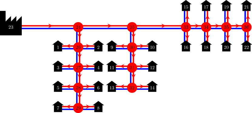
To illustrate the usefulness of the theoretical results, we consider district heating networks as a motivating example. Figure 1 shows a schematic example of such a system. Typically in existing networks of traditional design, one or a few large heating plants produce hot water which is pumped out to consumers via a network of pipelines (red edges in Figure 1). Each consumer is equipped with a valve to regulate the amount of hot water they receive. This water runs through a heat exchanger in which heat is transferred to the internal heating system of the building. The water subsequently returns through another network of pipes (blue edges in Figure 1) which is symmetric to the supply-side network. The primary aim in the network is to supply enough hot water to the consumers, such that they can maintain comfort temperatures within their buildings. We consider a simple dynamical model for the temperature in each building , which consumer would like to maintain at a reference temperature . Hence the tracking error is . The dynamics guiding the tracking error is thus given by
| (6) |
Here is the heat capacity of building . is the thermal conductance and is the outdoor temperature, acting as a disturbance. Hence the first term corresponds to diffusion of heat between the interior and exterior of the building. and are the specific heat capacity and density of water respectively (both assumed constant) and is the volume flow rate going through the building heat exchanger. is the difference in supply-and-return temperature before and after the heat exchanger. Hence the second term corresponds to the heat provided to the building through the heat exchanger. The volume flow rate is regulated by the valve positions . Note that the flow rate provided to consumer is influenced by the valve positions of all consumers in the network, not only . This is because the pressure distribution in the network is affected by all of the flow rates in the network. Herein lies the main connection to our theoretical results. As the central pump is limited in its maximum capacity, and the valves themselves are saturated, the volume flow rate and hence the heat that can be supplied to the consumers is limited. Hence when the disturbance is sufficiently low, the available capacity becomes insufficient.
To complete the connection between the temperature model (6) and the agent dynamics (1) as we have considered in this paper, we can identify , and . Secondly, we make the following simplifying assumption.
Assumption 4.
The delta temperatures , and are all constant.
In practice this assumption will not hold exactly. The delta temperature changes slightly with several factors, such as the supply-temperature in the network, the activity on the secondary side of the heat exchanger (i.e., the side facing the consumers internal heating system). There are also slight temperature-dependent variations in the density of the water. In general however and over shorter time-spans, these variations are much smaller than the variations in volume flow rate. This assumption means that the final verification to make is that satisfies Assumption 1. Under the assumption that we use common static models for the valves and pipes in the network such as in [24, 10, 25], that the network is tree-structured, and at the pump at the root of the tree operates at constant capacity, we can show the following. Hence satisfies Assumption 1.
Proposition 1.
Given two sets of valve positions ,
-
(i)
if , and
-
(ii)
if .
We omit the proof of this proposition, as it demands a technical description of district heating hydraulic models. However, we can motivate the proposition in the following way. If all agents incrementally open their valves (), this reduces the resistance in the system, which means that the total throughput increases (), i.e., . However, as the total throughput increases, so do pressure losses in the pipelines. Hence, if one valve is unchanged (), the flow rate through the valve will decrease due to reduced differential pressure (), i.e., .
4.1 Numerical Example
To investigate the effect of the considered control strategies in a district heating setting, we perform a simulation of a small district heating network. The network is structured as in Figure 1, and each building is subject to the dynamics given in (6). For simplicity, we consider a homogeneous building stock with , and . We have and . While we omit a detailed description of district heating hydraulics here, we use the same type of graph-based modeling as is used in [26]. We assume that the heating plant supplies a differential pressure of . The difference between the input and output of each pipe is given by where corresponds to a hydraulic resistance. We use for the long edge connecting nodes 23 and 24. We use for the edges connecting nodes 24, 25, 26, 30 and 33. We use for the pipes connecting nodes 26-27-28-29, nodes 30-31-32 and nodes 33-34-35-36. Finally we use for the connection to each consumer. The pressure difference between supply-and-return-side for consumer is modeled as . Here is limited in the . The component corresponds to inactive components of the consumer substation, i.e., the heat exchanger and internal piping. The remaining component corresponds to the pressure loss over the valve.
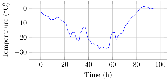
We subject the buildings to an outdoor temperatures disturbance as seen in Figure 2, acting equally on all buildings. The temperature drops critically to below C around 50 hours into the simulation. The temperature is based on temperature data from Gävle, Sweden on January 18th-21st, 2024. The data is collected from the Swedish Meteorological and Hydrological Institute.
We consider the two control policies analyzed in this paper, namely the decentralized and coordinating control policies. We employ identical controllers for each consumer with , , for all in the decentralized case, and , , , in the coordinating case. As a benchmark, we compare these strategies to optimal counter-parts. In these benchmarks, the volume flow rate is distributed optimally in each instance of the simulation as the solution to the problem {mini!} x,qJ(x) \addConstraint(6) with ˙x_i = 0 for i = 1,…,n \addConstraintq ∈Q where we use and respectively. This problem corresponds to calculating a flow rate which is feasible within the hydraulic constraints of the network (i.e., (2)) which generates an equilibrium (i.e., (2)) which minimizes . To see how this optimization problem can be cast as a convex problem, we refer to [10] in which it is shown that is convex.
We use the DifferentialEquations toolbox [27] in Julia to simulate the system, utilizing the FBDF solver. We use the NonlinearSolve [28] toolbox to calculate as a function of the valve positions . We use the Convex toolbox [29] with the Mosek optimizer to find the optimal trajectories for the benchmark comparisons.
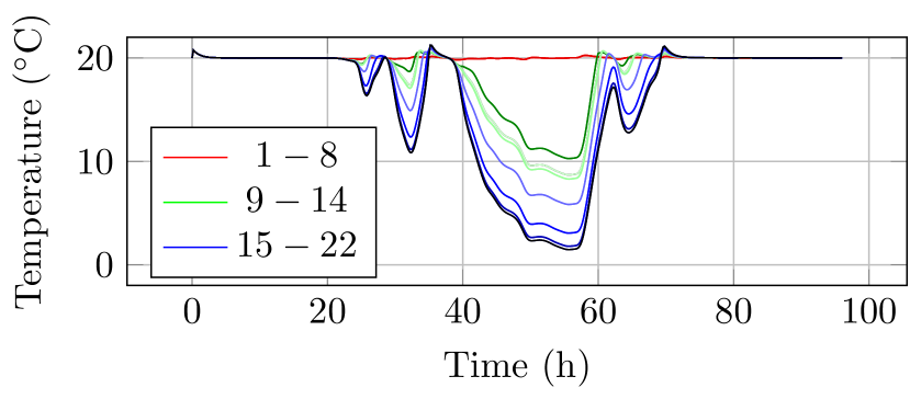
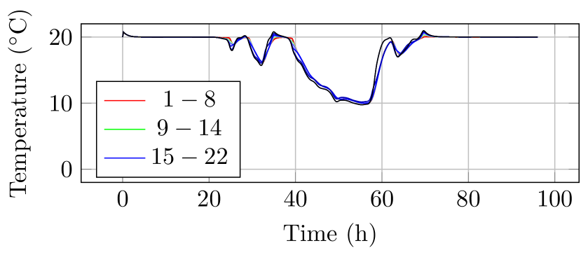
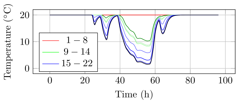
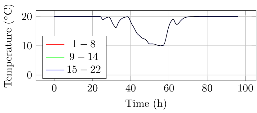
The results of the four simulations are seen in Figure 3. Under all four policies, the temperatures in the buildings drop at several points during the simulation, and most significantly starting after around 40 hours. This is because of the extremely cold temperature at this time, for which the available pumping capacity is insufficient. We can first compare the results of using the decentralized strategy to the results of using the optimal equilibrium input with regards to , as seen in Figures 3(a) and 3(c) respectively. We find that they are effectively the same, except for minor oscillations around the equilibrium in the PI-controller case, caused by the integral action in the controller. The same comparison can be drawn between Figures 3(b) and 3(d), showing the results of using the coordinating strategy and the optimal input with regards to . This is in line with Theorems 2 and 3, where we expect out controllers to track the optimal equilibrium. While the interpretation of the optimal cost in Theorem 2 is obscured by the weight , we see in this example how it can correspond to the combined tracking error of all agents .
When comparing the results of using the decentralized strategy to using the coordinating strategy, we see the following: In the fully decentralized simulation, several of the buildings far away from the heating plant drop below 5∘C, whereas buildings close to the heating facility maintain comfort temperature. On the other hand, none of the buildings drop below 10∘C. However, none of the buildings maintain comfort temperature either. Which strategy is to be preferred is debatable and perhaps situational. Arguably in the extreme scenario of this simulation, the decentralized strategy might be preferred. Consumers will be severely dissatisfied if their indoor temperatures drop by C, hence it may be better to have a lower number of consumers be very dissatisfied than to have the whole building stock be moderately dissatisfied. However, if we instead consider the temperatures distribution at around 30 hours into the simulations, we see that under the decentralized case there are buildings experiencing reductions in indoor temperature by C, whereas in the coordinated case the worst reduction is approximately C. In this case, it is arguably preferable to coordinate, as a C temperature reduction is acceptable for a shorter period of time, whereas C is too extreme to be tolerated by most consumers. The exact trade-offs and results will depend on the specific system and temperature levels at hand. What is interesting is that both of these behaviors which are optimal under different perspectives are achievable with such simple control techniques.
5 Main Proofs
We will now move on to prove the main theoretical results of this paper as presented in section 3. We will prove the stability results for both proposed controllers, i.e., Theorems 1 and 4, followed by the optimality of their equilibria, i.e., Theorems 2 and 3. First however, we will introduce a few extra properties of the interconnection which are required for the subsequent proofs.
5.1 Additional Nonlinearity Properties
The proofs of both of the following Lemmas are found in the Appendix.
Lemma 1.
Let satisfy Assumption 1. Consider any pair , where . Let and let . Then
| (7) |
This lemma is proven in the appendix. An interpretation of this lemma is that the individual change in output goes mostly along the same sign as the corresponding individual change in input . This value for all agents who have changed their inputs () dominates the change in output affecting all of the agents who did not change their inputs (). We continue with the following property of .
Lemma 2.
Let satisfy Assumption 1. Then for any pair and where , if , then .
This lemma is proven in the appendix. In the linear case where is an M-matrix (), this property can be likened with positivity of the inverse of this matrix ( element-wise).
5.2 Stability Proofs
We will prove both Theorem 1 and 4 using Lyapunov-based arguments. To do so, we will first introduce a change of coordinates from to , where and for . We also introduce the matrices , , and . Note that , , and are all positive definite, diagonal matrices under either Assumption 2 or Assumption 3. The closed-loop system in these new coordinates is then given by
| (8) |
Here denotes the anti-windup compensation, i.e., for the decentralized controller and for the coordinating controller.
We will first prove stability of the decentralized controller, beginning with ensuring that there exists an equilibrium.
Lemma 3.
This can be easily proven with Brouwer’s fixed-point theorem. We provide an outline of the proof in the Appendix, omitting the details for brevity. We can now prove stability of the decentralized closed-loop system.
Proof of Theorem 1.
Under the taken assumptions, Lemma 3 provides that the original system (2), and thus also (8), has at least one equilibrium which we denote . We introduce the shifted variables and , and the shifted notation , and . In this coordinate frame, the closed-loop dynamics are
| (9) |
The aim is now to show that (9) is globally, asymptotically stable with regards to the origin, which is equivalent with Theorem 1. Now recall the vector of Assumption 1, which we use to define the following Lyapunov function candidate.
| (10) |
While is not strictly continuously differentiable, we note this as a technicality. The function can be exchanged with an arbitrarily close approximation which is continuously differentiable in the origin. For this proof, we will maintain the convention that
| (11) |
Denote . We then find that
| (12a) | ||||
| (12b) | ||||
| (12c) | ||||
| (12d) | ||||
The terms (12a)–(12b) act fully diagonally, hence we can analyze their sign contribution for each individually. If either and or and , then clearly (12b) contributes with 0, and (12a) becomes strictly negative in the non-zero variable. If , then (12a) contributes with , but (12b) contributes with a negative semidefinite term, which is strictly negative if . If , (12b) contributes with a positive semidefinite term . However, in this case (12a) contributes with a strictly negative term . This negative term dominates the positive semidefinite term because of Assumption 2 where the anti-windup gain is bounded, and because . Hence the contribution of (12a)–(12b) is negative semidefinite, and strictly negative when . The term (12c) is trivially negative semidefinite, and strictly negative when . Finally, let . Note that , and if then either or . Hence the term (12d) can be bounded by
| (13) | ||||
| (14) | ||||
| (15) |
As Assumption 1 holds, we can employ Lemma 1 to show that this expression is strictly negative when . All together, if , we must have , or both, in which case will be negative due to the above arguments. If , the term (12a) is negative definite in . Hence is negative definite. As and for any non-zero pair the equilibrium is globally asymptotically stable for (8) and must therefore be unique. This can be translated to a unique equilibrium in the original coordinate frame, thus concluding the proof. ∎
To prove Theorem 3 regarding stability of the coordinating closed-loop system, we utilize the following result.
Lemma 4.
Proof.
For this proof, we will employ the coordinate frame as in (8), now with . Consider the Lyapunov function candidate
| (16) |
Here is to be understood to element-wise use the same bounds and as , i.e., if then . Note that
| (17) |
as when , and when . Hence we find that
| (18) | ||||
| (19) | ||||
| (20) | ||||
| (21) |
We will begin with the last term (21), which is strictly negative when . We can see this by noting that is a positive diagonal matrix, and then identifying that for any , if , , and thus Assumption 1 yields that
The opposite relation can be shown when . For the remaining terms, we first note that
| (22) |
which can trivially be shown by utilizing the definitions of and . Furthermore, Assumption 3 yields that and . Hence (18)–(20) can be combined and upper bounded by
This expression is negative semi-definite under the condition that . This is equivalent to
| (23) |
as is the Schur complement of this matrix. The condition (23) is once again equivalent to
| (24) |
This holds, due to Assumption 3. Hence and thus (18)–(20) is negative semi-definite. Therefore we have shown that when and when . Therefore the region where is globally attracting and forward invariant. ∎
Proof of Theorem 4.
Lemma 4 proves that all trajectories of the closed-loop system will converge to, and remain in, the region where . Here, the closed-loop systems of the coordinating and decentralized controllers are equivalent, and Assumption 3 implies that also Assumption 2 holds (disregarding the statements about the anti-windup gains, as they are inactive). Hence, we can invoke Theorem 1 which applies to the decentralized closed-loop system. ∎
5.3 Optimality Proofs
Proof of Theorem 2.
To simplify notation, we will introduce and . Note that by assumption. As both pairs and satisfy (1) with , we can conclude that
for all . Therefore
| (25) |
where and . As satisfies (2b) with , and , we know that . Hence we can continue to expand (25) to
| (26) |
We would here like to apply Lemma 1, but this requires the sets and . To continue, we note the following. For all , , and hence or . Therefore the following statements hold.
| (27) | |||||
| (28) | |||||
| (29) | |||||
| (30) | |||||
We can use these relations to reorganize and upper-bound the sums in (26), and therefore state that
| (31) |
The final inequality derives from Lemma 1, as we assume that Assumption 1 holds and . ∎
Proof of Theorem 3.
Since both and solve (1) with , we know that
| (32) |
where . We also know that
| (33) |
because is an equilibrium for the closed-loop system (4) and thus satisfy (4b) with . We therefore know that is proportional to the vector , and thus is maximized by all simultaneously. Consider first the case where . Then the contradictory notion that would therefore require that , and by (32) also . This is however impossible, because under Assumption 1, Lemma 2 states that requires . This is incompatible with (33), stating that , i.e., there must exist at least one such that , which means that necessarily , establishing a contradiction. We can make a symmetric argument to discard the possibility that and . Thus the only remaining option is , which requires , and thus , contradicting the assumption of the theorem statement. This concludes the proof. ∎
6 Conclusion
In this paper we considered a particular class of multi-agent systems, where the agents are connected through a capacity-constrained nonlinearity. For this type of system, we considered two proportional-integral controllers equipped with anti-windup compensation: One which was fully decentralized, and one in which the anti-windup compensator introduces a rank-1 coordinating term. We showed that the equilibria of these two closed-loop system were optimal, in the sense that they minimized the size of the control errors in terms of the costs and respectively. Additionally, we showed that the fully decentralized strategy provides guarantees of global, asymptotic stability with regards to a unique equilibrium. For the coordinating controller, we demonstrated global asymptotic stability when the disturbance can be rejected.
To demonstrate the applicability of the considered model, we showed how it can capture the indoor temperatures of buildings connected through a district heating network. In this setting, the capacity-constrained nonlinear interconnection consists of the hydraulics mapping the valve positions of each building to the resulting flow rates in the system. We demonstrated in a numerical example how the two considered controllers could then achieve different design goals - minimizing the average or the worst-case temperature deviations in the system respectively.
There are plenty of outlooks for future work: The internal agent dynamics are currently simple and on the form . This could perhaps be extended to more complex dynamics, where some stability assumptions are placed on the dynamics of each agent. Another outlook is analyzing the transient behavior of these systems. This would include understanding the effect of slowly time-varying and . In the district heating setting which we considered in this paper, this would account for changes in outdoor temperature and changes in the supply-temperature in the network. The cost-functions which are asymptotically minimized by the considered controllers could perhaps be generalized. Developments in this direction include design of controllers which maintain scalability and structure when considering other cost functions, as well as quantifying the suboptimality attained in utilizing one of the considered controllers in this paper for other cost functions. Finally, stronger stability guarantees can likely be established for the coordinating controller, which are applicable even when the stabilized equilibrium lies in the saturated domain.
7 Acknowledgments
This work is funded by the European Research Council (ERC) under the European Union’s Horizon 2020 research and innovation program under grant agreement No 834142 (ScalableControl).
The authors are members of the ELLIIT Strategic Research Area at Lund University.
References
- [1] F. P. Kelly, A. K. Maulloo, and D. K. H. Tan, “Rate control for communication networks: shadow prices, proportional fairness and stability,” Journal of the Operational Research Society, vol. 49, pp. 237–252, Mar. 1998.
- [2] S. Low and D. Lapsely, “Optimization flow control. I. Basic algorithm and convergence,” IEEE/ACM Transactions on Networking, vol. 7, pp. 861–874, Dec. 1999.
- [3] S. Low, F. Paganini, and J. Doyle, “Internet congestion control,” IEEE Control Systems Magazine, vol. 22, pp. 28–43, Feb. 2002.
- [4] F. Kelly, “Fairness and Stability of End-to-End Congestion Control*,” European Journal of Control, vol. 9, pp. 159–176, Jan. 2003.
- [5] E. Dall’Anese and A. Simonetto, “Optimal power flow pursuit,” IEEE Transactions on Smart Grid, vol. 9, no. 2, pp. 942–952, 2018.
- [6] D. K. Molzahn, F. Dörfler, H. Sandberg, S. H. Low, S. Chakrabarti, R. Baldick, and J. Lavaei, “A Survey of Distributed Optimization and Control Algorithms for Electric Power Systems,” IEEE Transactions on Smart Grid, vol. 8, pp. 2941–2962, Nov. 2017.
- [7] L. Ortmann, C. Rubin, A. Scozzafava, J. Lehmann, S. Bolognani, and F. Dörfler, “Deployment of an Online Feedback Optimization Controller for Reactive Power Flow Optimization in a Distribution Grid,” in 2023 IEEE PES Innovative Smart Grid Technologies Europe (ISGT EUROPE), (Grenoble, France), pp. 1–6, IEEE, Oct. 2023.
- [8] C. S. Kallesøe, B. K. Nielsen, A. Overgaard, and E. B. Sørensen, “A distributed algorithm for auto-balancing of hydronic cooling systems,” in 2019 IEEE Conference on Control Technology and Applications (CCTA), pp. 655–660, 2019.
- [9] C. S. Kallesøe, B. K. Nielsen, and A. Tsouvalas, “Heat balancing in cooling systems using distributed pumping,” IFAC-PapersOnLine, vol. 53, no. 2, pp. 3292–3297, 2020. 21st IFAC World Congress.
- [10] F. Agner, P. Kergus, R. Pates, and A. Rantzer, “Combating district heating bottlenecks using load control,” Smart Energy, vol. 6, 2022.
- [11] A. Martins, M. Lindberg, M. Maggio, and K.-E. Årzén, “Control-Based Resource Management for Storage of Video Streams,” IFAC-PapersOnLine, vol. 53, no. 2, pp. 5542–5549, 2020.
- [12] A. Martins and K.-E. Årzén, “Dynamic Management of Multiple Resources in Camera Surveillance Systems,” in 2021 American Control Conference (ACC), (New Orleans, LA, USA), pp. 2061–2068, IEEE, May 2021.
- [13] D. Krishnamoorthy and S. Skogestad, “Real-Time optimization as a feedback control problem – A review,” Computers & Chemical Engineering, vol. 161, p. 107723, May 2022.
- [14] A. Hauswirth, Z. He, S. Bolognani, G. Hug, and F. Dörfler, “Optimization algorithms as robust feedback controllers,” Annual Reviews in Control, vol. 57, p. 100941, 2024.
- [15] Z. He, S. Bolognani, J. He, F. Dörfler, and X. Guan, “Model-free nonlinear feedback optimization,” IEEE Transactions on Automatic Control, vol. 69, no. 7, pp. 4554–4569, 2024.
- [16] D. Bauso, F. Blanchini, L. Giarré, and R. Pesenti, “The linear saturated decentralized strategy for constrained flow control is asymptotically optimal,” Automatica, vol. 49, no. 7, pp. 2206–2212, 2013.
- [17] F. Blanchini, C. A. Devia, G. Giordano, R. Pesenti, and F. Rosset, “Fair and sparse solutions in network-decentralized flow control,” IEEE Control Systems Letters, vol. 6, pp. 2984–2989, 2022.
- [18] F. Agner, J. Hansson, P. Kergus, A. Rantzer, S. Tarbouriech, and L. Zaccarian, “Decentralized pi-control and anti-windup in resource sharing networks,” European Journal of Control, p. 101049, 2024.
- [19] F. Agner, P. Kergus, A. Rantzer, S. Tarbouriech, and L. Zaccarian, “Anti-windup coordination strategy around a fair equilibrium in resource sharing networks,” IEEE Control Systems Letters, vol. 7, pp. 2521–2526, 2023.
- [20] S. Galeani, S. Tarbouriech, M. Turner, and L. Zaccarian, “A tutorial on modern anti-windup design,” European Journal of Control, vol. 15, no. 3, pp. 418–440, 2009.
- [21] A. Hauswirth, F. Dörfler, and A. Teel, “On the robust implementation of projected dynamical systems with anti-windup controllers,” in 2020 American Control Conference (ACC), pp. 1286–1291, 2020.
- [22] R. A. Horn and C. R. Johnson, Topics in Matrix Analysis. Cambridge University Press, 1991.
- [23] R. Olfati-Saber and R. Murray, “Consensus problems in networks of agents with switching topology and time-delays,” IEEE Transactions on Automatic Control, vol. 49, no. 9, pp. 1520–1533, 2004.
- [24] C. De Persis, T. N. Jensen, R. Ortega, and R. Wisniewski, “Output Regulation of Large-Scale Hydraulic Networks,” IEEE Transactions on Control Systems Technology, vol. 22, pp. 238–245, Jan. 2014.
- [25] M. Jeeninga, J. E. Machado, M. Cucuzzella, G. Como, and J. Scherpen, “On the Existence and Uniqueness of Steady State Solutions of a Class of Dynamic Hydraulic Networks via Actuator Placement,” in 2023 62nd IEEE Conference on Decision and Control (CDC), pp. 3652–3657, Dec. 2023. ISSN: 2576-2370.
- [26] F. Agner, C. M. Jensen, A. Rantzer, C. S. Kallesøe, and R. Wisniewski, “Hydraulic parameter estimation for district heating based on laboratory experiments,” Energy, vol. 312, p. 133462, 2024.
- [27] C. Rackauckas and Q. Nie, “Differentialequations.jl–a performant and feature-rich ecosystem for solving differential equations in julia,” Journal of Open Research Software, vol. 5, no. 1, 2017.
- [28] A. Pal, F. Holtorf, A. Larsson, T. Loman, F. Schaefer, Q. Qu, A. Edelman, C. Rackauckas, et al., “Nonlinearsolve. jl: High-performance and robust solvers for systems of nonlinear equations in julia,” arXiv preprint arXiv:2403.16341, 2024.
- [29] M. Udell, K. Mohan, D. Zeng, J. Hong, S. Diamond, and S. Boyd, “Convex optimization in Julia,” SC14 Workshop on High Performance Technical Computing in Dynamic Languages, 2014.
Appendix: Remaining Proofs
Proof of Lemma 1..
Introduce the difference between the inputs as . We will then split the set into the two sets and . For all , we can invoke Assumption 1 to state that
| (34) |
Conversely, for any ,
| (35) |
Finally for all , Assumption 1 implies
| (36) |
Hence can expand (7) as
| (37) | ||||
| (38) | ||||
| (39) |
By Assumption 1 , this quantity is strictly positive when , which holds for any , thus concluding the proof.
∎
Proof of Lemma 2.
Let . Consider first the contradictory notion that . Then Assumption 1 yields that
| (40) |
Hence such that , and thus due to 1 we can conclude that . But since , we can also use Assumption 1 to find
| (41) |
This contradicts the assumption of the Lemma, and hence we conclude that . Therefore . Now consider the notion that such that . Then if , Assumption 1 states that , which contradicts the lemma assumption. Hence either or . Clearly is impossible, as this would contradict the assumption of the lemma. Thus .
∎
Proof sketch of Lemma 3..
An equilibrium with associated stationary control input satisfies (2) with . Note that to solve this system of equations, it is sufficient to find which satisfies
This uniquely fixes through (2a) and through (2c). Equation (Proof sketch of Lemma 3..) equates to solving a fixed-point problem , where we define the map as
where is chosen sufficiently small. is clearly forward-invariant with respect to a sufficiently large box of size , , which allows us to invoke Brouwer’s fixed-point theorem. ∎