Probing dark matter halo profiles with multi-band observations of gravitational waves

Abstract

In this paper, we evaluate the potential of multiband gravitational wave observations to constrain the properties of static dark matter spikes around intermediate-mass ratio inspirals. The influence of dark matter on the orbital evolution of the compact binary is incorporated as a correction to the inspiral Newtonian gravitational waveform. We show that the observations from the proposed space-based detector GWSat, sensitive within the deci-Hz frequency band, when combined with that of the third-generation ground-based detectors like the Einstein Telescope and Cosmic Explorer, will produce significantly improved error estimates for all parameters. In particular, our results demonstrate that the joint multiband approach substantially refines the bounds on the dark matter spike parameters-namely, the power-law index and spike density-by factors of approximately $10^{6}$ and $10^{3}$, respectively, compared to observations employing only third-generation gravitational wave detectors.

I Introduction

The direct observation of gravitational waves (GWs) has significantly enhanced our understanding of the universe, particularly in the study of black holes (BHs) and neutron stars (NSs). The detection of the first binary BH merger, GW150914, by the Laser Interferometer Gravitational-Wave Observatory (LIGO) in 2015 marked the beginning of GW astronomy [1], which has since led to a growing catalog of detected binary mergers. Looking ahead, the next generation of GW detectors promises to further expand our capabilities. Ground-based GW observatories such as the Cosmic Explorer (CE) [2] and Einstein Telescope(ET) [3], with their increased sensitivity, will enable the detection of fainter and more distant sources. Additionally, planned space-based detectors like LISA [4], DECIGO [5], and GWSat—a proposed Indian space-based GW detector—will aim to capture lower-frequency GW signals, particularly those emitted during the early inspiral phase of massive compact binary systems. These advancements in detector technology will provide a more complete picture of the universe’s compact objects and allow us to probe new physics, such as the nature of dark matter (DM), by exploring the environments in which these binaries exist. So far, most analyses of GW signals have assumed that source binaries evolve in vacuum environments, free from external perturbations. This assumption has served well for the initial detection of binary mergers by the LIGO-Virgo-KAGRA (LVK) collaboration [6, 7, 8, 9, 10], but it overlooks the possibility that many compact binaries could reside in dense astrophysical environments that might influence their orbital dynamics [11, 12]. Recent theoretical developments suggest that compact binaries, particularly those involving massive black holes, may be embedded in DM halos or other dense astrophysical structures [13]. Such environments could measurably impact the emitted GWs, altering the observed waveforms and providing indirect evidence of the presence and distribution of dark matter [14, 15, 16, 17, 18, 19, 20, 21, 22, 23, 24, 25, 26, 27, 28, 29, 30, 31, 32, 33, 34, 35, 36, 37, 38, 39, 40, 41, 42].

Navarro, Frenk, and White (NFW) were the first to demonstrate through cosmological N-body numerical simulations that DM halos possess a universal equilibrium density profile, commonly known as the NFW profile [43]. Subsequently, Gondolo and Silk indicated that the adiabatic growth of supermassive black holes (SMBHs) could significantly alter the surrounding DM distribution, leading to the formation of DM overdensities known as DM spikes [44]. However, host galaxy mergers and other astrophysical processes could disrupt these spike structures around SMBHs [45, 46, 47]. In contrast, intermediate-mass black holes (IMBHs), which have masses ranging from $10^{2}$ to $10^{5}\rm M_{\odot}$, are less likely to experience such disruptions, making them ideal candidates for investigating DM spikes [48, 49].

The existence of DM spikes can influence the orbital evolution of compact binaries. When a stellar-mass compact object inspirals around an IMBH embedded in a DM spike, it experiences not only the gravitational pull of the BH but also a drag force known as dynamical friction, which results from interactions with the dark matter spike [50, 51, 52]. This dynamical friction alters the binary’s inspiral rate, resulting in phase shifts in the gravitational waveform relative to what would be observed in a vacuum. Intermediate-mass ratio inspirals (IMRIs), which involve a stellar-mass object spiraling into an IMBH, are characterized by mass ratios in the range of $q=m_{2}/m_{1}\sim 10^{-3}-10^{-5}$, with $m_{1}$ and $m_{2}$ representing the masses of the IMBH and the smaller companion, respectively.

Space-based detectors such as LISA, DECIGO, and GWSat are going to be particularly valuable for detecting the early inspiral phase of IMRIs, during which the influence of the DM spike is most significant. These detectors operate in a lower frequency range (millihertz to decihertz) compared to ground-based detectors, making them ideal for capturing the initial stages of the inspiral when the orbital velocity is lower and the DM environment has a significant impact on the binary’s evolution. By combining data from both space-based and ground-based detectors—a technique known as multiband gravitational wave astronomy—it will be possible to track these systems across a broad range of frequencies, from the early inspiral phase to the final merger. This approach will significantly enhance parameter estimation and allow for more precise measurements of dark matter properties.

Multiband observations have been shown to dramatically enhance the precision of parameter estimation for compact binaries [53, 54]. Previous studies have primarily focused on stellar-mass binary black holes like GW150914, showing that multiband observations can improve signal-to-noise ratios by several orders of magnitude compared to single-band observations [53, 55, 56, 57]. In the case of IMRIs, the advantages of multiband detection are even more pronounced. IMRIs may produce detectable signals in both space-based and ground-based detectors, with signal-to-noise ratios of the order of hundreds to thousands in the space-based band (e.g., GWSat) and tens in the ground-based band (e.g., ET/CE). This complementary capability allows for reduced uncertainties in the measurement of key parameters [54], including the characteristics of DM spikes.

A recent study [35] conducted a Bayesian analysis of the first gravitational-wave catalog (GWTC-1) by LIGO-Virgo and found no significant evidence of environmental effects on the observed signals, but the results highlight the limitations of current detectors in detecting these subtle influences, particularly during the early inspiral phase where environmental effects are most likely to be identifiable. A numerical relativity study of GW150914-like events similarly suggests that environmental effects can mimic vacuum waveforms, potentially biasing parameter estimates [58]. Moreover, Ref. [59] demonstrated that using vacuum waveform templates for GW from inspirals in dark matter halos leads to biased parameter estimation, and suggests the necessity for an expanded parametrized post-Einsteinian (ppE) framework or more specialized DM waveform models.

In this work, we investigate the potential of multiband GW observations to measure the properties of static DM spikes around IMRIs using a Fisher analysis framework. We assess how the complementary sensitivities of space-based and ground-based detectors can significantly improve parameter estimation for both the vacuum and DM spike model parameters. Our results demonstrate that multiband observations provide significantly tighter constraints on the spike density and the power-law index compared to single-band observations, offering a promising avenue for probing dark matter environments around IMBHs.

This paper is structured as follows: In Sec. II, we describe the waveform models used for IMRIs in a DM environment and for parameter estimation. In Sec III, we outline the multiband Fisher analysis methodology. Sec. IV presents the results obtained, which is followed by concluding remarks in Sec. V. Throughout the paper, we adopt the geometrized units, where G = c = 1.

II Gravitational waves from the evolution of the IMRI in static dark matter spike

We consider an IMRI system comprising a stellar-mass compact object spiraling into an IMBH that is enveloped by a static DM spike, where the density profile remains constant over time. The mass of the IMBH is denoted by $m_{1}$, while the mass of the small compact object is indicated by $m_{2}$, and the orbital radius of the latter is symbolized by $r_{2}$. Initially, if the DM halo initially exhibits a cuspy profile $\rho(r)\propto r^{-\alpha}$ with $0\leq\alpha\leq 2$, this DM distribution will be altered due to adiabatic growth of the central IMBH, leading to the formation of a dense spike.

Following [16], we consider the spherically symmetric DM spike distribution with a simple power law:

$$\rho_{\text{DM}}(r)=\begin{cases}\rho_{\text{sp}}\left(\frac{r_{\text{sp}}}{r}\right)^{\gamma_{\text{sp}}}&\text{for }r_{\text{in}}\leq r\leq r_{\text{sp}}\\ 0&\text{for }r<r_{\text{in}}\end{cases},$$ (1)

where $r$ denotes the distance from the center of the IMBH. Following [60], we define the inner radius of the spike as $r_{\text{in}}=4Gm_{1}/c^{2}$. The maximum radius of the spike $r_{\mathrm{sp}}$ is determined by $r_{\mathrm{sp}}\sim 0.2r_{h}$, where $r_{h}$ is the radius of the gravitational influence of the central BH defined by

$$\int_{r_{\text{in}}}^{r_{h}}\rho_{\text{DM}}(r)\,d^{3}r=2m_{1}.$$ (2)

From this, the maximum radius of the spike $r_{\text{sp}}$ is determined as

$$r_{\text{sp}}\approx\left[\frac{(3-\gamma_{\text{sp}})0.2^{3-\gamma_{\text{sp}}}m_{1}}{2\pi\rho_{\text{sp}}}\right]^{1/3}.$$ (3)

The power-law index $\gamma_{\mathrm{sp}}$ that describes the final halo profile depends on the initial slope of the DM halo $\alpha$ which is related to the history of the formation of the IMBH via relation

$$\gamma_{\rm sp}=\frac{9-2\alpha}{4-\alpha}\,.$$ (4)

For the NFW profile, the initial slope is $\alpha=1$, henceforth the slope $\gamma_{\mathrm{sp}}=7/3=2.3\bar{3}$ is anticipated to form at the halo’s center [43]. Following the setting used in [16, 15], we set $\rho_{\mathrm{sp}}=226\mathrm{M}_{\odot}/\mathrm{pc}^{3}$ and $\gamma_{\mathrm{sp}}=7/3$ throughout this paper.

As a smaller compact object traverses a DM spike, the surrounding DM particles generate a disturbance that applies a drag force on it. This force reduces the smaller object’s orbital speed, resulting in energy loss via dynamical friction (DF) [50]. This energy dissipation hastens the orbital decay of the smaller body, causing it to spiral inward at a rate faster than in the absence of matter. Apart from DF, the system also loses energy through gravitational wave emission. The overall rate at which the system’s orbital energy decreases can be described as [22],

$$\frac{\mathrm{d}E_{\text{orb}}}{\mathrm{d}t}=-\frac{\mathrm{d}E_{\text{GW}}}{\mathrm{d}t}-\frac{\mathrm{d}E_{\text{DF}}}{\mathrm{d}t}.$$ (5)

The rate of energy loss due to GW emission for a circular orbit in the quadrupole approximation is expressed as [61]:

$$\frac{\mathrm{d}E_{\mathrm{GW}}}{\mathrm{d}t}=\frac{32G^{4}M(m_{1}m_{2})^{2}}{5(cr_{2})^{5}}.$$ (6)

The energy loss because of dynamical friction is given by [22, 50],

$$\frac{\mathrm{d}E_{DF}}{\mathrm{d}t}=4\pi(Gm_{2})^{2}\rho_{\mathrm{DM}}(r_{2})\xi(v)v^{-1}\log\Lambda,$$ (7)

where $v$ denotes the orbital velocity and the term $\xi(v)$ represents the fraction of dark matter particles with velocities lower than the orbital speed of the secondary object. As shown in [30], the factor $\xi$ is expressed as

$$\xi=1-I_{1/2}\left(\gamma_{sp}-\frac{1}{2},\frac{3}{2}\right),$$ (8)

where $I_{1/2}$ is the regularized incomplete beta function which estimated to be $\xi\approx 0.58$ for $\gamma_{\mathrm{sp}}=7/3$ as discussed in [21]. The notation $\log\Lambda$ refers to the Coulomb logarithm, defined by $\Lambda=\sqrt{m_{1}/m_{2}}$ as in [21]. This logarithm accounts for the range of proximities from the smaller mass where gravitational interactions with DM particles become significant.

By combining Eqs. (5) to (7), we can obtain the evolution of the orbital frequency and phase. For IMRIs on circular orbits in a static DM spike, the Newtonian-order time-domain phase left until coalescence as a function of the GW frequency $f$ as derived in [22], is given by

$$\Phi^{\mathrm{S}}(f)=\Phi^{\mathrm{V}}(f)$$ (9)

$$\quad\times{}_{2}\mathrm{F}_{1}\left(1,\frac{5}{11-2\gamma_{\mathrm{sp}}},1+\frac{5}{11-2\gamma_{\mathrm{sp}}},-c_{f}f^{-\frac{11-2\gamma_{\mathrm{sp}}}{3}}\right)\,.$$

Here ${}_{2}F_{1}(a,b,c,z)$ represents the Gaussian hypergeometric function, and $\Phi^{V}(f)$ is the phase for the system in vacuum with the chirp mass $\mathcal{M}=(m_{1}m_{2})^{3/5}/(m_{1}+m_{2})^{1/5}$ given by

$$\Phi^{V}(f)=\frac{1}{16}\left(\frac{1}{\pi\mathcal{M}f}\right)^{5/3}\,.$$ (10)

The coefficient $c_{f}$ is defined by [22],

$$c_{f}=\frac{5}{8m_{1}^{2}}\pi^{\frac{2(\gamma_{\mathrm{sp}}-4)}{3}}(m_{1}+m_{2})^{\frac{1-\gamma_{\mathrm{sp}}}{3}}r_{\mathrm{sp}}^{\gamma_{\mathrm{sp}}}\xi\rho_{sp}\log\Lambda.$$ (11)

The phase $\Phi^{\rm S}(f)$ nearly follows a broken power law, characterized by a break frequency $f_{\mathrm{eq}}$, where the energy loss rates from GWs and DF become equal, given by [22],

$$f_{\mathrm{eq}}=c_{f}^{\frac{3}{11-2\gamma_{\mathrm{sp}}}}.$$ (12)

Due to the DF effect, the inspiral process will involve fewer number cycles before coalescence, resulting in a gradual phase difference compared to a vacuum scenario. This phenomenon is referred to as dephasing, which can be mathematically expressed as: $\Delta\Phi=\Phi^{\rm V}-\Phi^{\rm S}$. The dephasing can be expanded above and below the $f_{\mathrm{eq}}$ as [22],

$$\Delta\Phi(f)=\begin{cases}\Phi^{\mathrm{V}}(f),&f\ll f_{\text{eq}}\\ \frac{5c_{f}\Phi^{\mathrm{V}}(f)}{2(8-\gamma_{sp})}f^{-\frac{11-2\gamma_{sp}}{3}},&f\gg f_{\text{eq}}\end{cases}.$$ (13)

Fig. 1 depicts the phase difference, $\Delta\Phi=\Phi^{\rm V}-\Phi^{\rm S}$, between an IMRI in a vacuum and one within a DM spike. It is observed that $\Delta\Phi$ increases at low frequencies. This behavior arises because of the gravitational impact on the orbiting object, which is governed by the mass of DM enclosed within the orbital radius. An increased enclosed mass results in a more pronounced phase shift. Since the lower GW frequencies are associated with larger orbits, the dephasing becomes significant at these lower frequencies. Therefore, it is crucial to consider observations from space-based detectors, which are sensitive in the mili-Hz and deci-Hz frequency ranges, to obtain better estimates of DM spike parameters such as $\rho_{\rm sp}$ and $\gamma_{\rm sp}$.

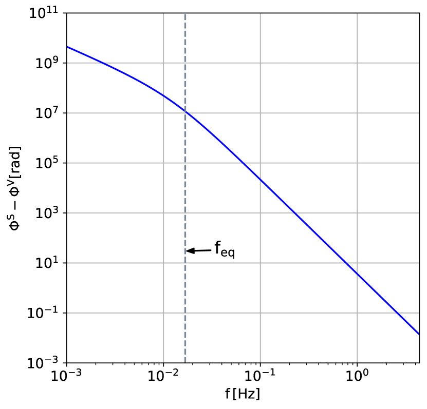
Figure 1: Following [22], we have shown the dephasing $\Delta\Phi$ vs frequency for IMRIs in static DM spike. The system considered here $(m_{1},m_{2},\rho_{\mathrm{sp}},\gamma_{\mathrm{sp}})=(400\mathrm{M}_{\odot},1.4\mathrm{M}_{\odot},226\mathrm{M}_{\odot}/\mathrm{pc}^{3},2.\bar{3})$ is different from [22]. The dashed line denotes the break frequency $f_{\mathrm{eq}}$ as defined in Eq. (12).

II.1 Gravitational-wave strain in the frequency domain

The binary system generates GWs due to variations in its quadrupole moment. Using the stationary phase approximation (SPA), the Fourier transform of the plus and cross-polarization waveforms can be expressed as [61]

$$\tilde{h}_{+,\times}(f)=A_{+,\times}(f)\,e^{i\,\Psi^{\rm S}(f)}$$ (14)

where the amplitudes of two polarizations at leading order are given by

$$A_{+}(f)= \frac{1}{D_{L}}\frac{(1+\cos^{2}{\iota})}{2}h_{0}(f),$$ (15)

$$A_{\times}(f)= \frac{1}{D_{L}}\cos{\iota}\,h_{0}(f),$$ (16)

$$h_{0}(f)= \sqrt{\frac{5}{24}}\frac{\mathcal{M}^{\frac{5}{6}}f^{-\frac{7}{6}}}{\pi^{\frac{2}{3}}}.$$ (17)

In these expressions, $D_{L}$ is the luminosity distance to the source, and $\iota$ represents the binary’s inclination angle. The frequency domain SPA phase $\Psi^{\rm S}(f)$ is related to the time domain phase, as a function of frequency by [22],

$$\Psi^{\rm S}(f)=2\pi f(t_{c}+t(f))-\phi_{c}-\frac{\pi}{4}+\Phi^{\rm S}(f).$$ (18)

where $t_{c}$ is the coalescence time, and $\phi_{c}$ is the phase at coalescence. The time evolution from an arbitrary initial frequency is given by

$$t(f)=\frac{1}{2\pi}\int\frac{\mathrm{d}f^{\prime}}{f^{\prime}}\frac{\mathrm{d}\Phi}{\mathrm{d}f}.$$ (19)

which for a system embedded in a static DM spike becomes [22]

$$t(f)=\frac{5a_{V}}{16\pi f^{8/3}}$$ (20)

$$\,\,\,\times{}_{2}F_{1}\left[1,\frac{8}{11-2\gamma_{sp}},1+\frac{8}{11-2\gamma_{sp}},-cf\,f^{\frac{2\gamma_{sp}-11}{3}}\right].$$

and for the vacuum case

$$t(f)=\frac{5a_{V}}{16\pi f^{8/3}}$$ (21)

with $a_{V}=\frac{1}{16}\left(\frac{1}{\pi\mathcal{M}}\right)^{5/3}$. Consequently, we write the frequency-domain phase for a system in a static DM spike as

$$\Psi^{\rm S}(f)=\Psi^{\mathrm{V}}(f)+\frac{3}{128\eta v^{5}}\left[p_{k_{1}}v^{k_{1}}+p_{k_{2}}v^{k_{2}}\right],$$ (22)

where $v\equiv(\pi Mf)^{1/3}$ and the symmetric mass ratio $\eta=m_{1}m_{2}/M^{2}$ where $M=m_{1}+m_{2}$ is the total mass of the binary. Furthermore, $\Psi^{\rm V}(f)$ represents the phase for the system in vacuum, given to leading post-Newtonian (PN) order by,

$$\Psi^{\rm V}(f)=2\pi ft_{c}-\phi_{c}-\frac{\pi}{4}+\frac{3}{128}(\pi\mathcal{M}f)^{-5/3}.$$ (23)

The second term in the right hand side of Eq. (22) shows the deviation from the vacuum phase due to the DF effect, where the dephasing parameters $p_{k_{1}}$ and $p_{k_{2}}$ are determined by

$$p_{k_{1}}= \frac{-20\,c_{f}\,(M\pi)^{\frac{11-2\gamma_{\mathrm{sp}}}{3}}}{(\gamma_{\mathrm{sp}}-8)(2\gamma_{\mathrm{sp}}-19)},$$ (24)

$$p_{k_{2}}= \frac{20\,{c_{f}}^{2}\,(M\pi)^{\frac{2(11-2\gamma_{\mathrm{sp}})}{3}}}{(2\gamma_{\mathrm{sp}}-15)(4\gamma_{\mathrm{sp}}-27)},$$ (25)

and the powers $k_{1}$ and $k_{2}$ depend on the spike power index $\gamma_{\mathrm{sp}}$ by

$$k_{1}=-11+2\gamma_{\mathrm{sp}},\quad k_{2}=2(-11+2\gamma_{\mathrm{sp}}).$$ (26)

In order to obtain the total phase in the static DM case in the form of Eq. (22), we expand the hypergeometric functions ${}_{2}F_{1}$ present in Eq. $(\ref{eq:Psi_S})$ up to the third order. For $2.25\leq\gamma_{\mathrm{sp}}\leq 2.5$, $-6.5\leq k_{1}\leq-6.0$, and $-4.5\leq k_{2}\leq-4.0$. Consequently, the correction to the vacuum phase due to the evolution of binary within the DM spike appears at a leading order compared to the (vacuum) GR contribution. Therefore, the environmental effects due to dark matter halo are more significant in the early inspiral phase when the binary system is evolving slowly.

The strain of GWs from the IMRI system measured by the detector in the frequency domain is given by the linear combination of the two GW polarizations $h_{+}$ and $h_{\times}$, given by [61],

$$\tilde{h}(f)=e^{i2\pi f\Delta t}\left(\,F_{+}(\lambda,\delta,\psi)\,\tilde{h}_{+}(f)+F_{\times}(\lambda,\delta,\psi)\,\tilde{h}_{\times}(f)\right).$$ (27)

Here, $\Delta t$ is the time delay between the arrival of a gravitational wave at the Earth’s center and the detector location. The antenna response functions $F_{+}$ and $F_{\times}$ determine the sensitivity of the detector to plus and cross polarizations, respectively. These functions are dependent on the sky position of the source, right ascension $\lambda$ and declination $\delta$, as well as polarization angle $\psi$.

III Multiband parameter estimation

III.1 Multiband Fisher analysis

The Fisher matrix is a widely-used approach for predicting the statistical uncertainties in GW parameter estimation when the models for both signal and noise are known [62, 63, 64]. In our analysis, we utilize the Fisher matrix approach to determine the $1\sigma$ uncertainties on both vacuum GR and dark matter model parameters.

The GW strain data $s(t)$ recorded by a detector is typically modeled as a combination of the true gravitational wave signal $h(t,\boldsymbol{\theta})$ embedded in additive detector noise $n(t)$:

$$s(t)=h(t,\boldsymbol{\theta})+n(t).$$ (28)

The likelihood function for the observed detector data, assuming stationary zero-mean Gaussian noise, is given by

$$\mathcal{L}\left(\boldsymbol{\theta}\right)=\exp\left(-\frac{1}{2}\left\langle s-h\left(\boldsymbol{\theta}\right)\mid s-h\left(\boldsymbol{\theta}\right)\right\rangle\right).$$ (29)

The Fisher Information Matrix (FIM) is defined as

$$\Gamma_{pq}=-\mathrm{E}\left[\frac{\partial^{2}\ln\mathcal{L}(\boldsymbol{\theta})}{\partial\theta_{p}\partial\theta_{q}}\right],$$ (30)

where E denotes the expectation value over the noise distribution. The Fisher information quantifies how much information an observable random variable (in our case, the noisy GW signal as observed by the detectors) provides about an unknown parameter or set of parameters. It may be seen as the curvature of the log-likelihood curve, with a high value indicating sharply peaked likelihood distribution, implying less variance on the maximum likelihood estimate of the parameters; and vice versa. One appeals to the Cramér–Rao [65] bound according to which, the inverse of the Fisher information provides a lower bound on the variance of any unbiased estimator of the parameters. As shown in [66], for a signal buried in stationary Gaussian noise, the FIM above given by Eq. (30) can be computed using the partial derivatives of the frequency-domain GW waveform with respect to the parameters:

$$\Gamma_{pq}=\left\langle\frac{\partial\tilde{h}(f)}{\partial\theta_{p}},\frac{\partial\tilde{h}(f)}{\partial\theta_{q}}\right\rangle,$$ (31)

where $\tilde{h}(f,\boldsymbol{\theta})$ is the frequency-domain GW waveform template defined by the set of parameters $\boldsymbol{\theta}$. The inner product between two functions, $a(f)$ and $b(f)$, weighted by the detector noise, is defined as:

$$\langle a,b\rangle=4\mathcal{R}\int_{f_{\rm low}}^{\rm f_{\rm high}}\frac{a(f)\,b^{*}(f)+a^{*}(f)\,b(f)}{S_{n}(f)}\,df\,,$$ (32)

where and “$*$” represents the complex conjugation, and $S_{n}(f)$ is the one-sided power spectral density (PSD) of the noise. The signal-to-noise ratio (SNR) for a given $\tilde{h}$ and a specific detector PSD $S_{n}(f)$ is given by

$$\rho=\langle\tilde{h},\tilde{h}\rangle^{1/2},$$ (33)

which indicates the relative strength of the detector response in relation to the detector noise. In the limit of high SNR, the inverse of the FIM provides the error covariance matrix $\Sigma_{pq}=(\Gamma_{pq})^{-1}$ and the square root of the diagonal elements of $\Sigma_{pq}$ gives the 1$\sigma$ error for each parameter: $\sigma_{p}=\sqrt{\Sigma_{pp}}$. In the case of multiband observations, where signals are detected jointly by both a space-based detector and a ground-based detector, the total FIM is obtained by summing the individual FIM from each detector [54]:

$$\Gamma^{\mathrm{Combined}}_{pq}=\sum_{j}\Gamma_{pq}^{j},$$ (34)

where $\Gamma_{pq}^{j}$ indicates the Fisher matrix associated with the j-th detector. The SNR for the network of detectors is defined as

$$\rho^{\rm Combined}=\sqrt{\sum_{j}{\rho^{j}}^{2}},$$ (35)

where $\rho^{j}$ denotes the SNR of j-th detector. Because these detectors are independently measuring the same event but under different conditions, the signals they capture are essentially independent pieces of data. This independence allows us to sum up their contributions. The covariance matrix for the combined measurement and the corresponding error estimate is given as [54],

$$\Sigma^{\mathrm{Combined}}_{pq}= (\Gamma^{\mathrm{Combined}}_{pq})^{-1},$$ (36)

$$\sigma^{\mathrm{Combined}}_{p}= \sqrt{\Sigma^{\mathrm{Combined}}_{pp}}.$$ (37)

When we sum the Fisher matrices from multiple detectors, the total information about the parameters increases, and as a result, the combined covariance matrix $\Sigma^{\mathrm{Combined}}_{pq}=(\Gamma^{\mathrm{Combined}}_{pq})^{-1}$ will typically have smaller diagonal elements than the covariance matrix of any individual detector. Hence, the uncertainties on the estimated parameters are reduced.

III.2 Detector configurations

We now focus on evaluating the detectability of GW signals originating from compact binary systems situated within dark matter environments, utilizing a consortium of proposed space-based detector GWSat, and 3G ground-based detectors, which include Cosmic Explorer (CE) and the Einstein Telescope (ET). This network of detectors is crucial for multiband GW observations, as it facilitates the detection of the same astrophysical source over a broad spectrum of frequencies, from the early inspiral phase through to the final merger and ringdown phases. CE is designed as a 40 km L-shaped detector, and it is expected to be sensitive to GWs within the frequency range of 5 Hz to 5 kHz. In contrast, ET features a triangular configuration with 10 km long arms and is anticipated to operate within a frequency range of 1 Hz to 5 kHz. Here, we set the locations of CE and ET as Idaho(USA) and Cascina(Italy), respectively.

On the other hand, GWSat is a proposed Indian space-based interferometer designed to detect GWs at low frequencies, specifically within the frequency range of 0.1 to 5 Hz. We consider GWSat as having an L-shaped configuration with an arm length $L=100$km and an opening angle of 90 degrees. The configuration is considered such that the vertex spacecraft follows a geostationary orbit around the Earth. For GWSat, the wavelengths of the GWs, $\lambda_{\mathrm{GW}}$ corresponding to its sensitive frequency range (0.1 to 5Hz) are of the order of $10^{5}$ to $10^{6}$ km. These wavelengths are significantly larger than the detector’s arm length $L$, which allows us to apply the long-wavelength approximation [67]. This long-wavelength approximation is also valid for ground-based detectors such as CE and ET. Therefore, we can use standard antenna pattern functions, similar to those utilized by ground-based detectors like LIGO, to characterize the sensitivity of GWSat, ET, and CE to gravitational waves coming from various directions. To characterize the sensitivity of GWSat, we adopt a placeholder noise PSD, given by [68]:

$$S_{n}(f)=(10^{-25}f^{-2}+10^{-23}f^{0}+10^{-24}f^{-1})^{2}\,\mathrm{Hz}^{-1}$$ (38)

This PSD serves as a notional model and is not derived from detailed noise source calculations; however, it is intended to approximate the expected sensitivity profile for GWSat.

III.3 Multiband visibility of IMRI system

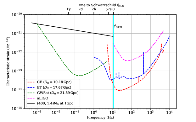
Figure 2: The dashed lines denote noise strain sensitivities of GWSat, aLIGO, CE, and ET. The solid black lines denote the characteristic amplitudes $(2\sqrt{f}|\tilde{h}(f)|)$ of an IMRI system in DM spike, with detector-frame masses 400$\mathrm{M}_{\odot}$ and 1.4$\mathrm{M}_{\odot}$ at 1 Gpc. $f_{\mathrm{ISCO}}$ for the considered system is shown by the cyan solid line. $D_{H}$ represents the horizon distance, which is the maximum observable distance for this IMRI system oriented face-on with respect to the detectors, at an SNR threshold of 10 for each detector. We have reproduced these curves using the PSDs for various detectors from [68, 69, 70, 71].

Now we discuss the SNR for various detectors. Fig. 2 shows the strain sensitivities of the GWSat, CE, ET, and aLIGO detectors along with the characteristic strain of the GW signal from an IMRI system in the DM spike. For the CE detector, we use the PSD of the 40km baseline CE detector [69], while for ET, we utilize the ET-D sensitivity [70]. For aLIGO, we take the sensitivity curve of the advanced design sensitivity aLIGOZeroDetHighPower [71]. The system under consideration consists of an IMRI with detector-frame companion masses of $400\rm M_{\odot}$ and $1.4\rm M_{\odot}$, located at a luminosity distance of $1\text{Gpc}$. The detector-frame masses are the redshifted source-frame masses given by $m_{z}=m_{\rm source}(1+z)$. This figure illustrates the frequency evolution of the IMRI system over time as the binary components spiral inward. The IMRI system remains detectable in the GWSat band for approximately one year before exiting the GWSat frequency range at 5 Hz. As it evolves, the system enters the ET and CE sensitivity ranges at 1 Hz and 5 Hz, respectively. Within the frequency interval between 1 Hz and 5 Hz, the GW signal becomes observable across both GWSat and ET detectors-facilitating simultaneous observation. Here we notice that the GW signal from the considered IMRI system will not be observable in the ground-based detector aLIGO.

The SNR values for the IMRIs that evolve in the DM environment as a function of detector-frame primary mass $m_{1}$ are illustrated in Fig. 3 for the GWSat, CE and ET detectors. In Fig. 3, the mass of the primary component $m_{1}$ is varied, while $m_{2}$ remains fixed at 1.4$\mathrm{M}_{\odot}$. The right ascension, declination, inclination angle, and polarization angle are all fixed to $\pi/4$. All sources are kept at a distance of $D_{L}=1$Gpc. The SNR in the CE and ET bands initially increases until the primary mass reaches the value of $150\mathrm{M}_{\odot}$ and $300\mathrm{M}_{\odot}$, respectively, and thereafter it begins to decrease. This reduction is attributed to the inspiral phase of the system becoming progressively shorter as the masses exceed these values.

The selection of the frequency bandwidth $(f_{\rm low},f_{\rm high})$ in integral Eq. (31) is contingent on the particular detector or the GW event being considered. The frequency cut-offs ($f_{\mathrm{min}}$, $f_{\mathrm{max}}$) for GWSat is chosen to be in the range of (0.1, 10) Hz. For the terrestrial detectors CE and ET, the corresponding cut-off frequencies are set to (5, 100) Hz and (1, 100) Hz, respectively. The choice of the low-frequency cut-off for IMRIs in the GWSat band depends on the duration for which the signal is expected to persist within that frequency range. We adopt a one-year observation period in the space-based GWSat band, and the lower cutoff frequency for the integral in Eq. (31) is chosen as

$$f_{\mathrm{low}}=\mathrm{max}(f_{\mathrm{year}},f_{\mathrm{min}}),$$ (39)

where $f_{\mathrm{year}}$ is the GW frequency one year before ISCO. This approach ensures that the frequency does not fall below the detector’s sensitivity range by taking the maximum value between $f_{\rm year}$ and $f_{\rm min}$. The GW frequency at a specific observation time $T_{\mathrm{obs}}$ before ISCO is determined using the quadrupole formula for radiation damping, as given in Eq. 2.15 of [72]:

$$f_{\mathrm{year}}=4.149\times 10^{-5}\left[\frac{\mathcal{M}_{z}}{10^{6}M_{\odot}}\right]^{-5/8}\left(\frac{T_{\mathrm{obs}}}{1\mathrm{yr}}\right)^{-3/8}\,.$$ (40)

The upper frequency limit for integration in Eq. (31) is chosen to be

$$f_{\mathrm{high}}=\mathrm{min}(f_{\mathrm{min}},f_{\mathrm{ISCO}}).$$ (41)

where $f_{\mathrm{ISCO}}$ is the Schwarzschild frequency of the innermost stable circular orbit of the compact binary coalescence given by [73]

$$f_{\mathrm{ISCO}}=\frac{1}{6^{3/2}\pi M_{z}},$$ (42)

where $M_{z}$ is the detector-frame total mass of the compact binary system.

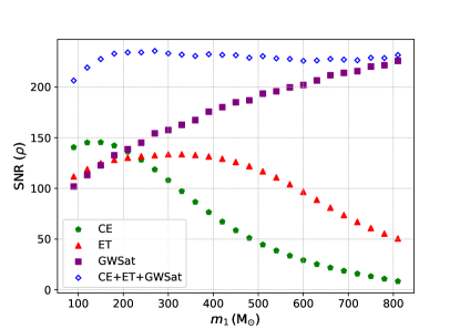
Figure 3: SNR from IMRIs in DM spike profile accumulated across the frequency bands of GWSat, CE, ET, as well as for combined CE+ET+GWSat observations up until $f_{\rm ISCO}$, as a function of detector-frame primary mass $m_{1}$. The detector-frame secondary mass $m_{2}$ is set to 1.4$\mathrm{M}_{\odot}$. All the IMRI sources are considered to be located at 1 Gpc.

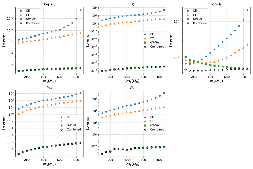
Figure 4: The bounds on various vacuum as well as DM model parameters as a function of the primary mass $m_{1}$ in the detector frame. The detector-frame secondary mass $m_{2}$ is kept constant at $1.4\mathrm{M}_{\odot}$, with all IMRIs systems considered to be situated at a luminosity distance of 1Gpc. The diamond-shaped markers symbolize the combined bounds achieved through multiband observations incorporating GWSat, CE, and ET detectors.

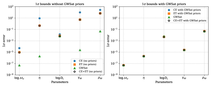
Figure 5: Comparison of 1$\sigma$ bounds on parameters for IMRI system of detector-frame masses 400$\mathrm{M}_{\odot}$ and 1.4$\mathrm{M}_{\odot}$ at 1 Gpc in a dark matter spike environment, using ground-based detectors (CE, ET, and CE+ET) with and without the addition of priors from GWSat. The left panel shows the 1$\sigma$ bounds on parameters estimated independently from CE, ET, and CE+ET, as well as from GWSat alone. The right panel incorporates priors on parameters $\{\log{\mathcal{M}_{z}},\eta,\log{D_{L}},\gamma_{\rm sp},\rho_{\mathrm{sp}}\}$ obtained from GWSat’s extended observation in the deci-Hz frequency band, showing significant improvement in parameter constraints when combined with CE and ET observations.

III.4 Setup for Fisher analysis

The parameter vector $\boldsymbol{\theta}$ for Fisher analysis depends on the waveform model used. To estimate the errors on parameters for an IMRI system in DM spike, we choose the following parameter space:

$$\boldsymbol{\theta}=\{\log{\mathcal{M}_{z}},\eta,\log{D_{L}},\gamma_{\rm sp},\rho_{\mathrm{sp}}\}.$$ (43)

We calculate statistical uncertainties for various IMRI systems and ground-based and space-based GW detectors, utilizing GWBENCH [74], a Python-based tool designed to calculate the covariance matrix and $1\sigma$ errors on the parameters. The plus and cross polarizations for the waveform for the static DM scenario are incorporated within the GWBENCH framework for this analysis. The frequency cut-offs used for the integration in Eq. (31) for the estimation of errors are the same as mentioned in Section III.3. The fiducial value of chirp mass $\mathcal{M}_{z}$ in the detector-frame is calculated using the detector-frame secondary mass $m_{2}=1.4\mathrm{M}_{\odot}$ and different values of detector frame primary BH mass $m_{1}$. The fiducial value of $D_{L}$ is fixed to be 1Gpc. Additionally, the fiducial values for the right ascension, declination, inclination angle, and polarization angle are set to $\pi/4$.

When estimating the uncertainties of the parameters using Fisher analysis, we also consider the impact of Earth’s rotation on the antenna patterns and responses of the detector. This consideration is especially important for GW signals that last a long time within the detector’s bandwidth, as the source’s position in the sky can change significantly due to Earth’s rotation relative to the detector on Earth.

IV Results

In this section, we demonstrate the results of our analysis in detail. The $1\sigma$ bounds on various parameters using only GWSat, only CE, only ET, and multiband (GWSat + CE + ET) observations are presented in Fig. 4 for various values of detector-frame primary mass $m_{1}$. The secondary object’s mass is fixed at $1.4\mathrm{M}_{\odot}$, and the binaries are located at the luminosity distance of $1$Gpc.

The analysis reveals that combining space-based and ground-based detector observations significantly improves the bounds on all parameters compared to using CE or ET observations alone. The errors obtained from CE and ET increase with increasing total mass. This occurs because, as the total mass increases, the signal spends less time within the sensitivity range of CE and ET. The bounds obtained on parameters $\log{\mathcal{M}_{z}}$, $\eta$, $\log{D_{L}}$, $\gamma_{\rm sp}$, and $\rho_{\mathrm{sp}}$ from GWSat overall remains comparable with increase in $m_{1}$. As illustrated in Fig. 4, CE and ET alone offer relatively poor bounds on both the power-law index $\gamma_{\rm sp}$ and the spike density $\rho_{\mathrm{sp}}$, across the entire range of analyzed range of $m_{1}$. This limitation arises because ground-based detectors are more sensitive to the later stages of the inspiral, where the influence of the surrounding DM is less pronounced.

In contrast, GWSat, with its prolonged observation duration during the early inspiral phase, captures the environmental effects of the DM spike in the low-frequency regime. This improvement highlights the significance of multiband observations in accurately estimating the DM spike characteristics, as data from GWSat complement the high-frequency precision provided by CE and ET during the later stages of the inspiral and subsequent merger. Moreover, the error estimates for $\gamma_{\rm sp}$ and $\rho_{\mathrm{sp}}$ show significant improvement when joint observations via both space-based and ground-based detectors are implemented, with an improvement of the order of approximately $10^{6}$ and $10^{3}$, respectively, relative to observations conducted solely with CE or ET detectors.

The constraints on the parameters are obtained from long-duration observations in the space-based GWSat band can be utilized to enhance parameter estimation in ground-based detectors like CE and ET. The early inspiral phase of the IMRI system observed over a year in the deci-Hz frequency range, allows for precise determination of certain parameters before the system transitions to higher frequencies. These constraints from early detection can then be incorporated as priors when estimating parameter uncertainties in ground-based detectors, which capture the high-frequency signal during the late inspiral and merger phases. By adding these priors, derived from the Fisher matrix analysis of GWSat data, to the Fisher matrix of CE/ET, we can significantly reduce parameter uncertainties.

To illustrate the influence of incorporating priors from GWSat’s observations, Fig. 5 presents a comparative view of the 1$\sigma$ errors on various parameters of the IMRI system in a dark matter spike environment. The left panel shows the 1$\sigma$ bounds estimated independently from ground-based detectors (CE, ET, and their combined observation CE+ET) without the use of priors. The right panel incorporates the effect of adding priors on the parameters $\{\log{\mathcal{M}_{z}},\eta,\log{D_{L}},\gamma_{\rm sp},\rho_{\mathrm{sp}}\}$—derived from GWSat’s year-long observation during the inspiral phase of the IMRI system—into the Fisher matrices of CE and ET.

From Fig. 5, it is evident that incorporating priors on the parameters $\{\log{\mathcal{M}_{z}},\eta,\log{D_{L}},\gamma_{\rm sp},\rho_{\mathrm{sp}}\}$ from space-based observations significantly improves the parameter constraints obtained from ground-based detectors. Specifically, the 1$\sigma$ bounds on the DM spike model parameters $\gamma_{\rm sp}$ and $\rho_{\mathrm{sp}}$ for CE and ET detectors improve by factors of approximately $10^{6}$ and $10^{4}$, respectively, when priors from GWSat observations are included. These improvements occur because these parameters are well constrained in the deci-Hz frequency band. Additionally, the pre-existing parameter constraints obtained from GWSat observations play a critical role in refining source localization for ground-based detectors like CE and ET, particularly for observing the later stages of compact binary coalescence.

V Conclusion

In this paper, we investigated the capability of multiband gravitational wave observations to constrain the properties of static dark matter spikes around IMRIs using a Fisher analysis framework. Specifically, we studied IMRI systems embedded in static dark matter spike profiles and examined how multiband observations, combining space-based and 3G ground-based detectors, can improve the estimation of both vacuum and dark matter parameters.

The study focused on systems characterized by varying masses of the primary black hole and fixed secondary mass of $1.4\mathrm{M}_{\odot}$. We incorporated the effects of dynamical friction which gives rise to the correction to the inspiral part of the Newtonian GW waveform phase in relation to the vacuum phase. This effect appears at the leading order into the GW phase compared to the leading contribution coming from GR, rendering them significant during the early inspiral phase of the binary system. For these effects to be detectable, they must accumulate over many orbital cycles, which primarily occur during the extended inspiral phase. Therefore, it is crucial to consider observations from future space-based detectors, as they will capture the accumulated effects of dark matter over a significant number of cycles from the IMRIs. By utilizing the complementary sensitivity of space-based detectors such as GWSat and 3G ground-based detectors like CE and ET, we achieved significantly better error estimates on the static dark matter spike parameters, including the spike density $\rho_{\mathrm{sp}}$ and the power-law index $\gamma_{\rm sp}$, compared to individual detectors alone.

We showed that while CE and ET when used independently, provide limited constraints on the parameters $\gamma_{\rm sp}$ and $\rho_{\rm{sp}}$, incorporating GWSat in a multiband approach yields substantial improvements in parameter estimation. In particular, our results demonstrated that the joint multiband approach enhances the constraints on $\gamma_{\rm sp}$ and $\rho_{\mathrm{sp}}$ by factors of approximately $10^{6}$ and $10^{3}$, respectively, relative to observations with only ground-based detectors. Moreover, the addition of priors on the parameters obtained from the GWSat observations while estimating errors with CE and ET significantly improves the bounds on the parameters.

However, the IMRI systems are highly asymmetric, and the contribution of higher modes becomes important for more accurate estimations of the parameter uncertainty. We would like to explore the effects of the contribution of the higher modes to our analysis in a future study. Also, it will be interesting to extend our analysis for eccentric orbits and for spinning binaries. Furthermore, we like to extend our studies to effective field theory models of dark matter (e.g., the one considered [32]). For this, we need to systematically compute the GW phase and carry out the Fisher analysis. Last but not least, we like to perform a thorough Bayesian analysis to get a more realistic bound on the dark matter parameter using multi-band observations. We hope to report on it soon.

VI Acknowledgements

A.B like to thank the speakers and the participants of the (virtual) workshop “Testing Aspects of General Relativity-II”, “Testing Aspects of General Relativity-III” and “New insights into particle physics from quantum information and gravitational waves” at Lethbridge University, Canada funded by McDonald Research Partnership-Building Workshop grant by McDonald Institute for valuable discussions. A.B is supported by the SERB Core Research Grant (CRG/2023/005112) by DST-ANRF of India Govt. A.B also acknowledges the associateship program of the Indian Academy of Sciences, Bengaluru. D.T. would like to acknowledge the support of the Inspire fellowship from the Department of Science and Technology of India under fellowship number DST/INSPIRE Fellowship/[IF210643].

References

- Abbott et al. [2016] B. P. Abbott et al. (LIGO Scientific Collaboration and Virgo Collaboration), Phys. Rev. Lett. 116, 061102 (2016).
- Reitze et al. [2019] D. Reitze et al., Bull. Am. Astron. Soc. 51, 035 (2019), eprint 1907.04833.
- Punturo et al. [2010] M. Punturo et al., Class. Quant. Grav. 27, 194002 (2010).
- Amaro-Seoane et al. [2017] P. Amaro-Seoane et al. (LISA) (2017), eprint 1702.00786.
- Yagi and Seto [2011] K. Yagi and N. Seto, Phys. Rev. D 83, 044011 (2011), [Erratum: Phys.Rev.D 95, 109901 (2017)], eprint 1101.3940.
- Abbott et al. [2019a] B. P. Abbott et al. (LIGO Scientific, Virgo), Phys. Rev. X 9, 031040 (2019a), eprint 1811.12907.
- Abbott et al. [2021] R. Abbott et al. (LIGO Scientific, Virgo), Phys. Rev. X 11, 021053 (2021), eprint 2010.14527.
- Abbott et al. [2023a] R. Abbott et al. (KAGRA, VIRGO, LIGO Scientific), Phys. Rev. X 13, 041039 (2023a), eprint 2111.03606.
- Abbott et al. [2019b] B. P. Abbott et al. (LIGO Scientific, Virgo), Astrophys. J. Lett. 882, L24 (2019b), eprint 1811.12940.
- Abbott et al. [2023b] R. Abbott et al. (KAGRA, VIRGO, LIGO Scientific), Phys. Rev. X 13, 011048 (2023b), eprint 2111.03634.
- Barausse et al. [2014] E. Barausse, V. Cardoso, and P. Pani, Phys. Rev. D 89, 104059 (2014), eprint 1404.7149.
- Barausse et al. [2015] E. Barausse, V. Cardoso, and P. Pani, J. Phys. Conf. Ser. 610, 012044 (2015), eprint 1404.7140.
- Merritt et al. [2002] D. Merritt, M. Milosavljevic, L. Verde, and R. Jimenez, Phys. Rev. Lett. 88, 191301 (2002), eprint astro-ph/0201376.
- Macedo et al. [2013] C. F. B. Macedo, P. Pani, V. Cardoso, and L. C. B. Crispino, Astrophys. J. 774, 48 (2013), eprint 1302.2646.
- Eda et al. [2013] K. Eda, Y. Itoh, S. Kuroyanagi, and J. Silk, Phys. Rev. Lett. 110, 221101 (2013), eprint 1301.5971.
- Eda et al. [2015] K. Eda, Y. Itoh, S. Kuroyanagi, and J. Silk, Phys. Rev. D 91, 044045 (2015), eprint 1408.3534.
- Yue and Han [2018] X.-J. Yue and W.-B. Han, Phys. Rev. D 97, 064003 (2018), eprint 1711.09706.
- Yue et al. [2019] X.-J. Yue, W.-B. Han, and X. Chen, Astrophys. J. 874, 34 (2019), eprint 1802.03739.
- Hannuksela et al. [2020] O. A. Hannuksela, K. C. Y. Ng, and T. G. F. Li, Phys. Rev. D 102, 103022 (2020), eprint 1906.11845.
- Cardoso and Maselli [2020] V. Cardoso and A. Maselli, Astron. Astrophys. 644, A147 (2020), eprint 1909.05870.
- Kavanagh et al. [2020] B. J. Kavanagh, D. A. Nichols, G. Bertone, and D. Gaggero, Phys. Rev. D 102, 083006 (2020), eprint 2002.12811.
- Coogan et al. [2022] A. Coogan, G. Bertone, D. Gaggero, B. J. Kavanagh, and D. A. Nichols, Phys. Rev. D 105, 043009 (2022), eprint 2108.04154.
- Liu et al. [2021] D. Liu, Y. Yang, S. Wu, Y. Xing, Z. Xu, and Z.-W. Long, Phys. Rev. D 104, 104042 (2021).
- Zhang et al. [2021] C. Zhang, T. Zhu, and A. Wang, Phys. Rev. D 104, 124082 (2021).
- Becker and Sagunski [2023] N. Becker and L. Sagunski, Phys. Rev. D 107, 083003 (2023), eprint 2211.05145.
- Baryakhtar et al. [2022] M. Baryakhtar et al., in Snowmass 2021 (2022), eprint 2203.07984.
- Cardoso et al. [2022] V. Cardoso, K. Destounis, F. Duque, R. Panosso Macedo, and A. Maselli, Phys. Rev. Lett. 129, 241103 (2022), eprint 2210.01133.
- Singh et al. [2023] D. Singh, A. Gupta, E. Berti, S. Reddy, and B. S. Sathyaprakash, Phys. Rev. D 107, 083037 (2023), eprint 2210.15739.
- Destounis et al. [2023] K. Destounis, A. Kulathingal, K. D. Kokkotas, and G. O. Papadopoulos, Phys. Rev. D 107, 084027 (2023), eprint 2210.09357.
- Nichols et al. [2023] D. A. Nichols, B. A. Wade, and A. M. Grant, Phys. Rev. D 108, 124062 (2023), eprint 2309.06498.
- Chowdhuri et al. [2024] A. Chowdhuri, R. K. Singh, K. Kangsabanik, and A. Bhattacharyya, Phys. Rev. D 109, 124056 (2024), eprint 2306.11787.
- Bhattacharyya et al. [2023] A. Bhattacharyya, S. Ghosh, and S. Pal, JHEP 08, 207 (2023), eprint 2305.15473.
- Rahman et al. [2024] M. Rahman, S. Kumar, and A. Bhattacharyya, JCAP 01, 035 (2024), eprint 2306.14971.
- Duque et al. [2024a] F. Duque, C. F. B. Macedo, R. Vicente, and V. Cardoso, Phys. Rev. Lett. 133, 121404 (2024a), eprint 2312.06767.
- Caneva Santoro et al. [2024] G. Caneva Santoro, S. Roy, R. Vicente, M. Haney, O. J. Piccinni, W. Del Pozzo, and M. Martinez, Phys. Rev. Lett. 132, 251401 (2024), eprint 2309.05061.
- Speeney et al. [2024] N. Speeney, E. Berti, V. Cardoso, and A. Maselli, Phys. Rev. D 109, 084068 (2024), eprint 2401.00932.
- Aurrekoetxea et al. [2024] J. C. Aurrekoetxea, J. Marsden, K. Clough, and P. G. Ferreira, Phys. Rev. D 110, 083011 (2024), eprint 2409.01937.
- Zhang et al. [2024] C. Zhang, G. Fu, and N. Dai, JCAP 04, 088 (2024), eprint 2401.04467.
- Bertone et al. [2024] G. Bertone, A. R. A. C. Wierda, D. Gaggero, B. J. Kavanagh, M. Volonteri, and N. Yoshida (2024), eprint 2404.08731.
- Spieksma et al. [2024] T. F. M. Spieksma, V. Cardoso, G. Carullo, M. Della Rocca, and F. Duque (2024), eprint 2409.05950.
- Duque et al. [2024b] F. Duque, S. Kejriwal, L. Sberna, L. Speri, and J. Gair (2024b), eprint 2411.03436.
- Cheng et al. [2024] Y.-Z. Cheng, Y. Cao, and Y. Tang (2024), eprint 2411.03095.
- Navarro et al. [1997] J. F. Navarro, C. S. Frenk, and S. D. M. White, Astrophys. J. 490, 493 (1997), eprint astro-ph/9611107.
- Gondolo and Silk [1999] P. Gondolo and J. Silk, Phys. Rev. Lett. 83, 1719 (1999), eprint astro-ph/9906391.
- Ullio et al. [2001] P. Ullio, H. Zhao, and M. Kamionkowski, Phys. Rev. D 64, 043504 (2001), eprint astro-ph/0101481.
- Vasiliev and Zelnikov [2008] E. Vasiliev and M. Zelnikov, Phys. Rev. D 78, 083506 (2008), eprint 0803.0002.
- Bertone and Merritt [2005] G. Bertone and D. Merritt, Mod. Phys. Lett. A 20, 1021 (2005), eprint astro-ph/0504422.
- Zhao and Silk [2005] H.-S. Zhao and J. Silk, Phys. Rev. Lett. 95, 011301 (2005), eprint astro-ph/0501625.
- Bertone et al. [2005] G. Bertone, A. R. Zentner, and J. Silk, Phys. Rev. D 72, 103517 (2005), eprint astro-ph/0509565.
- Chandrasekhar [1943] S. Chandrasekhar, Astrophys. J. 97, 255 (1943).
- Ostriker [1999] E. C. Ostriker, Astrophys. J. 513, 252 (1999), eprint astro-ph/9810324.
- Kim and Kim [2007] H. Kim and W.-T. Kim, Astrophys. J. 665, 432 (2007), eprint 0705.0084.
- Sesana [2016] A. Sesana, Phys. Rev. Lett. 116, 231102 (2016), eprint 1602.06951.
- Datta et al. [2021] S. Datta, A. Gupta, S. Kastha, K. G. Arun, and B. S. Sathyaprakash, Phys. Rev. D 103, 024036 (2021), eprint 2006.12137.
- Barausse et al. [2016] E. Barausse, N. Yunes, and K. Chamberlain, Phys. Rev. Lett. 116, 241104 (2016), eprint 1603.04075.
- Gnocchi et al. [2019] G. Gnocchi, A. Maselli, T. Abdelsalhin, N. Giacobbo, and M. Mapelli, Phys. Rev. D 100, 064024 (2019), eprint 1905.13460.
- Grimm and Harms [2020] S. Grimm and J. Harms, Phys. Rev. D 102, 022007 (2020), eprint 2004.01434.
- Roy and Vicente [2024] S. Roy and R. Vicente (2024), eprint 2410.16388.
- Wilcox et al. [2024] E. Wilcox, D. Nichols, and K. Yagi (2024), eprint 2409.10846.
- Sadeghian et al. [2013] L. Sadeghian, F. Ferrer, and C. M. Will, Phys. Rev. D 88, 063522 (2013), eprint 1305.2619.
- Maggiore [2007] M. Maggiore, Gravitational Waves. Vol. 1: Theory and Experiments (Oxford University Press, 2007), ISBN 978-0-19-171766-6, 978-0-19-852074-0.
- Cramér [1946] H. Cramér, Mathematical Methods in Statistics (Pergamon Press, Princeton University Press, NJ, U.S.A., 1946).
- Cutler and Flanagan [1994] C. Cutler and E. E. Flanagan, Phys. Rev. D 49, 2658 (1994), eprint gr-qc/9402014.
- Vallisneri [2008] M. Vallisneri, Phys. Rev. D 77, 042001 (2008), eprint gr-qc/0703086.
- Kotz and Johnson [1991] S. Kotz and N. Johnson, eds., Breakthroughs in Statistics. Springer Series in Statistics (Springer, New York, 1991), chap. Information and the Accuracy Attainable in the Estimation of Statistical Parameters, pp. 235–247, v. 1-2.
- HELSTROM [1968] C. W. HELSTROM, in Statistical Theory of Signal Detection (Second Edition) (Pergamon, 1968), International Series of Monographs in Electronics and Instrumentation, pp. 249–289, second edition ed., ISBN 978-0-08-013265-5, URL https://www.sciencedirect.com/science/article/pii/B9780080132655500148.
- Jaranowski and Krolak [2005] P. Jaranowski and A. Krolak, Living Rev. Rel. 8, 3 (2005), eprint 0711.1115.
- [68] Private communication with Sanjit Mitra, IUCAA, Pune, India.
- Srivastava et al. [2022] V. Srivastava, D. Davis, K. Kuns, P. Landry, S. Ballmer, M. Evans, E. D. Hall, J. Read, and B. S. Sathyaprakash, Astrophys. J. 931, 22 (2022), eprint 2201.10668, URL https://cosmicexplorer.org/sensitivity.html.
- Hild et al. [2011] S. Hild et al., Class. Quant. Grav. 28, 094013 (2011), eprint 1012.0908, URL https://www.et-gw.eu/index.php/etsensitivities.
- [71] L. Barsotti, S. Gras, M. Evans, and P. Fritschel, The updated advanced ligo design curve, ligo technical note t1800044-v5 (ligo scientific collaboration, 2018) updated from t0900288-v3, URL https://dcc.ligo.org/LIGO-T1800044/public.
- Berti et al. [2005] E. Berti, A. Buonanno, and C. M. Will, Phys. Rev. D 71, 084025 (2005), eprint gr-qc/0411129.
- Cutler and Vallisneri [2007] C. Cutler and M. Vallisneri, Phys. Rev. D 76, 104018 (2007), eprint 0707.2982.
- Borhanian [2021] S. Borhanian, Class. Quant. Grav. 38, 175014 (2021), eprint 2010.15202.