Unsupervised Machine Learning for Classifying CHIME Fast Radio Bursts and Investigating Empirical Relations

Abstract

Fast Radio Bursts (FRBs) are highly energetic millisecond-duration astrophysical phenomena typically categorized as repeaters or non-repeaters. However, observational limitations may lead to misclassifications, suggesting a larger proportion of repeaters than currently identified. In this study, we leverage unsupervised machine learning techniques to classify FRBs using data from the CHIME/FRB catalog, including both the first catalog and a recent repeater catalog. By employing Uniform Manifold Approximation and Projection (UMAP) for dimensionality reduction and clustering algorithms (k-means and HDBSCAN), we successfully segregate repeaters and non-repeaters into distinct clusters, identifying over 100 potential repeater candidates. Our analysis reveals several empirical relations within the clusters, including the ${\rm log\,}\Delta t_{sc}-{\rm log\,}\Delta t_{rw}$, ${\rm log\,}\Delta t_{sc}-{\rm log\,}T_{B}$, and $r-\gamma$ correlations, which provide new insights into the physical properties and emission mechanisms of FRBs. This study demonstrates the effectiveness of unsupervised learning in classifying FRBs and identifying potential repeaters, paving the way for more precise investigations into their origins and applications in cosmology. Future improvements in observational data and machine learning methodologies are expected to further enhance our understanding of FRBs.

1 Introduction

Fast Radio Bursts (FRBs) are highly energetic astronomical phenomena characterized by millisecond-duration emissions. The first FRB signal was discovered in 2007 by Lorimer et al. (2007), and their existence was firmly established in 2013 when Thornton et al. (2013) published observations of four similar events detected by the Australian Parkes Radio Telescope. Since then, FRBs have drawn significant attention in both astronomy and cosmology (e.g., Lorimer, 2018; Keane, 2018; Petroff et al., 2022; Xiao et al., 2021; Xiao & Dai, 2022; Xiao et al., 2022; Zhang, 2014; Zhang & Li, 2018; Zhang et al., 2021; Zhang & Zhang, 2022; Wang et al., 2020a, b; Wang & Zhang, 2019; Wang & Wei, 2023; Gao et al., 2014; Qiang & Wei, 2020, 2021). However, the origin of FRBs remains unknown.

To explore their origin, numerous radio telescopes have been constructed, such as, the Deep Synoptic Array (DSA; J. et al., 2019; Hallinan et al., 2019), Arecibo (Spitler et al., 2014), Parkes (e.g., Lorimer et al., 2007; Burke-Spolaor & Bannister, 2014; Petroff et al., 2015; Ravi & Lasky, 2014), the Canadian Hydrogen Intensity Mapping Experiment (CHIME; CHIME/FRB Collaboration et al., 2018), the Five-hundred-meter Aperture Spherical Radio Telescope (FAST; Li & Pan, 2016), and the Australian Square Kilometer Array Pathfinder (ASKAP; Shannon et al., 2024). So far, nearly a thousand FRBs have been observed(Petroff et al., 2016; CHIME/FRB Collaboration et al., 2021; Jankowski et al., 2023; Xu et al., 2023), with nearly 100 of them have known redshifts (e.g. Law et al., 2024; Sharma et al., 2024; Bhardwaj et al., 2024; Gordon et al., 2023). To date, the largest FRB sample is the first CHIME/FRB catalog (CHIME/FRB Collaboration et al., 2021).

In astronomical observations, the measured quantities are often influenced by the distance between the source and Earth. Therefore, distance-related information is crucial for analyzing the origin of FRBs. A key observational parameter correlated with distance for FRBs is the Dispersion Measure (DM), which quantifies the total column density of free electrons along the line of sight between the source and the observer. For the vast majority of observed FRBs, the DM values significantly exceed the predicted values for their respective directions within the Milky Way, indicating that these FRBs originate from distant extragalactic regions of the universe. Meanwhile, an FRB event, FRB 20200428, was observed to have originated within the Milky Way, providing evidence that at least some FRBs are associated with magnetars (Andersen et al., 2020; Li et al., 2021a; Bochenek et al., 2020; Lin et al., 2020).

Based on the observational characteristics, FRBs are broadly classified into two categories, i.e., repeaters and non-repeaters. As the names suggest, repeaters are sources that have exhibited multiple bursts, whereas non-repeaters have only been observed once. Since the discovery of the first repeater, FRB 20121102 (Spitler et al., 2016), more than 50 FRBs have been identified as repeaters to date (CHIME/FRB Collaboration et al., 2021, 2023; Kumar et al., 2019; Kirsten et al., 2022; Fonseca et al., 2020; Niu et al., 2022; Xu et al., 2022), while most of the remaining ones are classified as non-repeaters. However, Ravi (2019) suggests that the volumetric rate of non-repeating FRBs might exceed that of cataclysmic events and the formation rate of compact objects, implying that the majority of FRBs should be repeaters. Some studies also propose that more than half of the FRBs in the first CHIME/FRB catalog could be repeaters (Yamasaki et al., 2023; McGregor & Lorimer, 2024). Furthermore, several FRBs initially identified as non-repeaters were later observed to show repeating characteristics (CHIME/FRB Collaboration et al., 2023). This suggests that many of the FRBs currently classified as non-repeaters might actually be potential repeaters, with only a single burst detected due to various observational factors. As a result, some studies have attempted to identify potential repeaters among apparent non-repeating FRBs, and one of the methods being employed is machine learning.

Machine learning is an artificial intelligence technique that allows computers to learn from data and make predictions or decisions without being explicitly programmed (Cover & Hart, 1967; Rumelhart et al., 1986). Machine learning is generally categorized into three types, i.e., supervised learning, unsupervised learning, and semi-supervised learning (e.g. Dempster et al., 2018; Breiman, 2001; Chang & Lin, 2011; Vapnik, 1999). Using algorithms to uncover patterns in the data can be applied to tasks such as classification, regression, clustering, and optimization. Until now, machine learning has already been widely used in the detection and analysis of FRBs (e.g. Wagstaff et al., 2016; Zhang et al., 2018; Wu et al., 2019; Yang et al., 2021; Adámek & Armour, 2020; Agarwal et al., 2020; Bhatporia et al., 2023). For instance within the first CHIME/FRB catalog dataset, Chen et al. (2021) and Zhu-Ge et al. (2022) identify 188 and 117 repeater candidates from 474 non-repeating FRBs via unsupervised learning, correspondingly. Yang et al. (2023) instead discovered 145 repeater using FRB morphology as features, while Luo et al. (2022) identified dozens of repeater candidates with varies supervised learning methods. Furthermore, Luo et al. (2022) found that the most prominent factors to distinguish between non-repeating and repeating FRBs are brightness temperature and rest-frame frequency bandwidth, whereas Sun et al. (2024) found spectral running may play a role instead. Furthermore, some studies have used machine learning techniques to classify thousands of bursts from highly active repeaters, such as FRB 20121102 (Raquel et al., 2023) and FRB 20201124A (Chen et al., 2023), in an effort to analyze their potential radiation mechanisms.

In addition to classifying FRBs based on their repeatability, some studies have also investigated the clustering of FRBs using characteristics beyond repeatability, as well as the empirical relationships among these features. For instance, similar to the well-known classification of GRB, where short GRBs are short lived and associated with old population, while long GRB with long duration and associated with young population (Zhang et al., 2007; Kumar & Zhang, 2014), Guo & Wei (2022) proposed classifying FRBs based on their association with either old or young stellar populations. They discovered several tight empirical relations for non-repeaters in the first CHIME/FRB catalog, such as ${\rm log\,}E-{\rm log\,}L_{\nu}$, ${\rm log\,}E-{\rm log\,DM_{E}}$ and ${\rm log\,DM_{E}}-{\rm log\,}L_{\nu}$, where ${\rm log\,}$ means the logarithm to base 10, and $E$, ${\rm DM_{E}}$, $L_{\nu}$ are isotropic energy, spectral luminosity, and extragalactic DM, respectively. Similar empirical relations were found for non-repeaters associated with old populations and all non-repeaters, though with notably different slopes and intercepts, such as ${\rm log\,}F_{\nu}-{\rm log\,}S_{\nu}$, ${\rm log\,DM_{E}}-{\rm log\,}S_{\nu}$, and ${\rm log\,}F_{\nu}-{\rm log\,DM_{E}}$, where $F_{\nu}$ is specific fluence, $S_{\nu}$ is flux. Many empirical relations still hold for localized FRBs (Li et al., 2024). Based on these empirical relations, FRBs could potentially serve as standard candles, allowing cosmological models to be constrained without relying on DM measurements (Guo & Wei, 2024). Li et al. (2021b) classified FRBs into short ($W<100\,$ms) and long ($W>100\,$ms) bursts, where $W$ represents the pulse width. A strong power-law correlation between fluence and peak flux density was identified for these categories. Xiao & Dai (2022) classified repeating FRBs into classical ($T_{B}\geq 10^{33}\,$K) and atypical ($T_{B}<10^{33}\,$K) bursts, where $T_{B}$ refers to the brightness temperature. A tight power-law correlation between pulse width and fluence was also observed for classical bursts.

CHIME has recently released a new repeater catalog (CHIME/FRB Collaboration et al., 2023), significantly increasing the data available on repeaters. This expanded dataset is expected to improve the accuracy of identifying repeater candidates through machine learning. In this paper, we will apply unsupervised learning methods to classify the FRBs from the combined data of these two catalogs into different clusters, find potential repeaters among the non-repeaters, and analyze possible empirical relations across these clusters. This paper is structured as follows. In Section 2, we present the selected CHIME data and the features used in our analysis. introduces two types of unsupervised machine learning methods, i.e., dimensionality reduction and clustering, as well as evaluation metrics. In Section 4, we present the results of dimensionality reduction and clustering, then we analyze the potential empirical relations. Finally, Section 5 provides our conclusions.

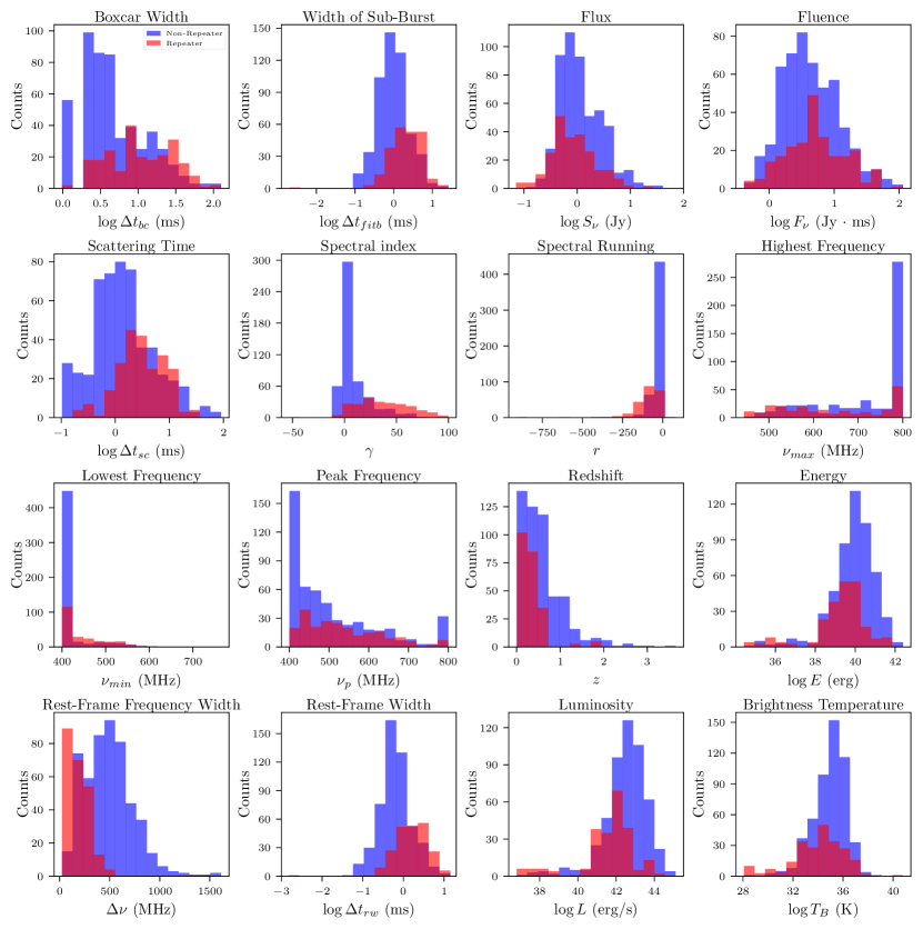
Figure 1: The distributions of observed and derived parameters for non-repeaters and repeaters are shown separately, forming the input data used for unsupervised learning. For more details, refer to Section 2.

2 DATA SET

2.1 Sample Construction

In this paper, we use the largest available FRB data from CHIME to date, including the first CHIME/FRB Catalog (CHIME/FRB Collaboration et al., 2021, here after Cat1) and the CHIME/FRB Collaboration (2023) Catalog (CHIME/FRB Collaboration et al., 2023, here after Cat2023). The Cat1 including 536 events (474 non-repeaters and 62 repeat bursts from 18 repeaters), all events have 600 sub-bursts because of multiple peaks appearing in the light curve of FRB. The Cat2023 contains 127 events from 39 repeaters , or 151 sub-bursts for all events. Since there are 6 FRBs in Cat1 with flux and fluence values of zero, we excluded those FRBs. Additionally, 6 non-repeaters in Cat1, identified as repeaters, are duplicates in Cat2023, resulting in 739 FRB bursts used in this paper.

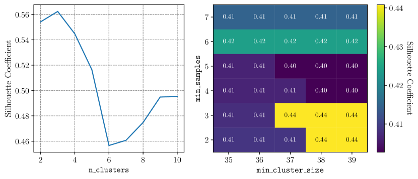
Figure 2: The mean silhouette coefficients of the k-means (left panel) and HDBSCAN (right panel) with respect to different hyperparameters.

2.2 Feature Selection

Based on these data, we choose the parameters of the sub-bursts as the features for machine learning algorithms. To provide a more comprehensive description of an FRB event, we selected as many parameters as possible to serve as features. These parameters can be divided into two categories: observational parameters (original data provided by Cat1 and Cat2023) and derived parameters, and we present the distribution of all parameters for the entire FRB dataset in Figure 1. We chose 10 observational parameters as did by Chen et al. (2022):

• Boxcar width $\Delta t_{bc}$ (ms) – The boxcar width of sub-burst, with the label name ‘bc_width’ in two catalogs.

• Width of sub-burst $\Delta t_{fitb}$ (ms) – The width of sub-burst that is fitted by fitburst , with the label name ‘width_fitb’ in two catalogs.

• Flux $S_{\nu}$ (Jy) – The peak flux of the band-average profile (lower limit) with the label name ‘flux’ in two catalogs.

• Fluence $F_{\nu}$ ($\rm Jy\cdot ms$) – The flux integrated over the duration of sub-burst (lower limit) with the label name ‘fluence’ in two catalogs.

• Scattering time $\Delta t_{sc}$ (ms) – The scattering time at 600 MHz of each sub-burst, with the label name ‘scat_time’ in two catalogs.

• Spectral index $\gamma$ – The spectral shape parameter of sub-burst. The label name in two catalogs is ‘sp_idx’.

• Spectral running $r$ – This value characterizes the frequency dependence of the spectral shape and is labeled as ‘sp_run’ in both catalogs.

• Highest frequency $\nu_{max}$ (MHz) – The highest frequency band of detection for the sub-burst at full-width tenth-maximum. The label name in two catalogs is ‘high_freq’.

• Lowest frequency $\nu_{min}$ (MHz) – The lowest frequency band of detection for the sub-burst at full-width tenth-maximum. The label name in two catalogs is ‘low_freq’.

• Peak frequency $\nu_{p}$ (MHz) – The peak frequency for the sub-burst and is labeled as ‘peak_freq’ in both catalogs.

For $\Delta t_{bc}$, $\Delta t_{fitb}$, $S_{\nu}$, $F_{\nu}$, and $\Delta t_{sc}$, we take their logarithmic values throughout this work. Cat1 and Cat2023 only provide upper limits for the width of sub-burst and scattering time for some FRBs, so we opted to use these upper limits in our analysis.

For the derived parameters, we choose 6 physical properties of FRBs (see more details in Zhu-Ge et al., 2023):

• Redshift $z$ – The redshift of FRBs is numerically derived from their dispersion measure (DM).

  The FRB can be separated into different components (see e.g. Deng & Zhang, 2014; Gao et al., 2014; Zhou et al., 2014; Yang et al., 2017; Yang & Zhang, 2016; Li et al., 2019; Wei et al., 2019; Qiang et al., 2020; Qiang & Wei, 2020, 2021; Qiang et al., 2022):

  $${\rm DM_{obs}=DM_{MW}+DM_{halo}+DM_{IGM}+DM_{host}}/(1+z),$$ (1)

  where $\rm DM_{MW},DM_{halo},DM_{IGM}$ and $\rm DM_{host}$ represent the contributions from the Milky Way, the Milky Way halo, the intergalactic medium (IGM), and the host galaxy (including interstellar medium of the host galaxy and the plasma around source) of the FRB. In the literature, we usually use extragalactic DM for research

  $${\rm DM_{E}=DM_{obs}-DM_{MW}-DM_{halo}=DM_{IGM}+DM_{host}}/(1+z).$$ (2)

  In this paper, the values $\rm DM_{obs}$ are provided by both catalogs with label name ‘bonsai_dm’. We used the values of $\rm DM_{MW}$ as provided in Cat1 and Cat2023, which were estimated using the NE2001 model (Cordes & Lazio, 2002)(the corresponding label names in Cat1 and Cat2023 are ‘dm_exc_ne2001’ and ‘dm_exc_1_ne2001’, respectively). Following the previous studies, we adopt ${\rm DM_{halo}}=30$ $\rm pc\hskip 2.40005ptcm^{-3}$ and ${\rm DM_{host}}=70$ $\rm pc\hskip 2.40005ptcm^{-3}$ . For the $\rm DM_{IGM}$, it can be written as (see e.g. Deng & Zhang, 2014; Yang & Zhang, 2016; Li et al., 2019; Wei et al., 2019; Qiang et al., 2020; Qiang & Wei, 2020, 2021; Qiang et al., 2022)

  $${\rm DM_{IGM}}(z)=\frac{3cH_{0}\Omega_{b,0}}{8\pi Gm_{p}}\int_{0}^{z}\frac{f_{\rm IGM}(\tilde{z})\,f_{e}(\tilde{z})\left(1+\tilde{z}\right)d\tilde{z}}{E(\tilde{z})},$$ (3)

  where $c$ is the speed of light, $G$ is the gravitational constant, $m_{p}$ is the mass of proton, $E(z)$ is the dimensionless Hubble parameter. For cosmological parameters, we adopt $H_{0}=67.4$ $\rm km\hskip 2.40005pts^{-1}\hskip 2.40005ptMpc^{-1}$ , $\Omega_{m}=0.315$ and $\Omega_{b,0}h^{2}=0.0224$ from latest Planck 18 results for the flat $\Lambda$CDM cosmology (Planck Collaboration et al., 2020). $f_{e}(z)$ is the ionized electron number fraction per baryon, and $f_{\rm IGM}(z)$ is the fraction of baryon mass in IGM. In principle, these two parameters are functions of redshift z. In this work, we follow e.g. Qiang et al. (2020); Qiang & Wei (2021); Gao et al. (2014); Yang et al. (2017) and use the fiducial values $f_{e}=0.875$ and $f_{\rm IGM}=0.83$. According to Eq.2 and Eq. 3, we can derive the redshift of all FRBs. Following Zhu-Ge et al. (2023), we also set minimum redshift of 0.002248 corresponding to a luminosity distance of 10 Mpc to avoid zero or negative values.

• Rest-frame frequency width $\Delta\nu$ (MHz) – The frequency width corrected for the cosmological redshift effect, it can be calculated by

  $$\Delta\nu=(\nu_{max}-\nu_{min})(1+z).$$ (4)

• Rest-frame width $\Delta t_{rw}$ (ms) – The width of sub-burst $\Delta t_{fitb}$corrected for the cosmological redshift effect: $\Delta t_{rw}$ = $\Delta t_{fitb}$$/(1+z)$. We take the logarithmic values.

• Burst energy $E$ (erg) – The energy of FRB can be calculated by

  $$E=\frac{4\pi d_{L}^{2}}{1+z}F_{\nu}\nu_{p},$$ (5)

  where $d_{L}$ is the luminosity distance. We take their logarithmic values.

• Luminosity $L$ (erg/s) – The luminosity of FRBs can be derived from

  $$L=4\pi d_{L}^{2}S_{\nu}\nu_{p},$$ (6)

  and we take the logarithmic values.

• Brightness temperature $T_{B}$ (K) – The brightness temperature can be derived as

  $$T_{B}=\frac{S_{\nu}d_{L}^{2}}{2\pi\kappa_{B}(\nu_{p}\Delta t_{fitb})^{2}}=1.1\times 10^{35}\,{\rm K}\,\left(\frac{S_{\nu}}{\rm Jy}\right)\,\left(\frac{d_{L}}{\rm Gpc}\right)\,\left(\frac{\nu_{p}}{\rm GHz}\right)^{-2}\,\left(\frac{\Delta t_{fitb}}{\rm ms}\right)^{-2},$$ (7)

  where $\kappa_{B}$ is the Boltzmann constant. We take the logarithmic values.

3 Method

Dimensionality reduction and clustering are two types of unsupervised machine learning methods used in this paper. First, we apply the dimensionality reduction algorithm to automatically convert high-dimensional data into low-dimensional data. Then, we use a clustering algorithm to classify the reduced-dimensional data based on their similarities.

3.1 Machine Learning Techniques

3.1.1 Dimensionality Reduction

In this study, we use Uniform Manifold Approximation and Projection (UMAP, McInnes et al., 2018), implemented via the python package umap-learn , to perform dimensionality reduction. UMAP is a dimensionality reduction technique that can be used for both visualization and general nonlinear dimensionality reduction. This algorithm assumes that the input data is uniformly distributed on a Riemannian manifold with a locally constant (or approximately constant) Riemannian metric and that the manifold is locally connected. Based on these assumptions, the manifold can be modeled using a fuzzy topological structure.

The use of UMAP has been extensively explored in many studies. For FRB classification, the three parameters n_compnent, n_neighbors, and min_dist have a more significant impact on the classification results. Meanwhile, we also experimented with modifying other parameters and found that they had minimal effect on the classification outcomes. Therefore, in this study, we choose to focus on adjusting these three parameters of UMAP. n_compnent allows us to determine the dimensionality of the reduced space where the data will be embedded. In our work, we set $\mathtt{n\_compnent}=2$ for all features, projecting the data onto a 2D plane for visual representation.n_neighbors controls how UMAP balance the local and globol structure of data. UMAP achieves this by controlling the size of the local neighborhood it considers when attempting to learn the underlying structure of the data. This means that low values of n_neighbors will cause UMAP to focus on very local structures, potentially at the cost of missing the overall global structure. On the other hand, higher values of n_neighbors will push UMAP to consider larger neighborhoods around each point, capturing the broader structure of the data, but possibly losing finer details. min_dist decides how tightly UMAP can pack points together in low-dimensional space. Basically, it sets the minimum distance between points in the low-dimensional space. Lower values of min_dist will lead to more tightly packed, “clumpier” embeddings, which can be beneficial for identifying clusters or preserving finer topological details. In contrast, higher values of min_dist will prevent the points from being tightly packed, instead focusing on maintaining the broader topological structure. We scan n_neighbors from 2 to 50 and min_dist from 0.0 to 0.99. In this paper, we take n_neighbors = 21, and min_dist = 0.03.

3.1.2 Clustering Algorithms

In this work, we used k-means (MacQueen et al., 1967; Lloyd, 1982) and Hierarchical Density-Based Spatial Clustering of Applications with Noise (HDBSCAN Campello et al., 2013, 2015; McInnes et al., 2017) to group the reduced-dimensional data into different clusters. K-means clustering is based on the distance between each data point and its corresponding cluster center. It aims to minimize the distance between the points and their respective centers, effectively grouping similar points into clusters based on proximity in the feature space. Initially, the k-means algorithm selects k random points as the initial cluster centers, calculates the Euclidean distance of each data point from these centers, and assigns each point to the nearest center. Then, it recalculates the mean of each cluster, updating the cluster centers. This process is repeated iteratively until the cluster centers stabilize, minimizing the overall variance within the cluster (for detals, see Fotopoulou, 2024, and reference their in). We use sklearn.cluster.KMeans  to perform the k-means clustering algorethm. The essential hyperparameter is n_clusters, it means how many clusters are present in the model.

HDBSCAN is a clustering algorithm developed by Campello et al. (2013, 2015). It extends Density-based Spatial Clustering of Applications with Noise (DBSCAN, Ester et al., 1996) by transforming it into a hierarchical clustering method (Han et al., 2012). The algorithm then extracts flat clusters from this hierarchy based on the stability of the clusters, which allows it to better handle varying densities and identify clusters of different shapes and sizes. HDBSCAN uses minimum spanning trees, allowing it to discover clusters with varying densities, unlike DBSCAN, which assumes a constant density across the entire dataset. This flexibility enables HDBSCAN to identify clusters of different shapes and sizes, making it more adaptable to complex structures. We use a python package hdbscan  to perform this clustering algorithm. The hyperparameters of HDBSCAN adjusted in this paper are min_cluster_size and min_samples. min_cluster_size controls the minimum number of points required to form a cluster, while min_samples determines how conservative the algorithm is in classifying points as noise or part of a cluster. These parameters directly influence the number of clusters and the overall shape of the clustering.

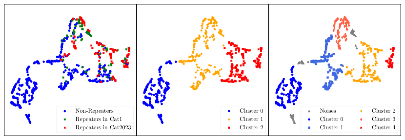
Figure 3: The results of dimensionality reduction and clustering. Left panel: The distribution of UMAP-embedded data. Blue dots represent non-repeaters, while green and red crosses indicate repeaters from Cat1 and Cat2023, respectively. Middle panel: The clustring result of UMAP-embedded data from k-measn. Cluster 0, 1, and 2 are represented by blue dots, orange stars, and red crosses, respectively. Right panel: The clustring result of UMAP-embedded data from HDBSCAN. Gray triangles, blue dots, royal blue squares, orange stars, tomato diamonds, and red crosses represent Noise, and Cluster 0, 1, 2, 3, and 4, respectively.

Algorithm	Cluster	Non-repeater number	Repeater number	Repeater candidate number	Total number	Repeater precentage	Recall	Repeating rate
K-means	Cluster 0	210	0	0	210	0%	100%	61.7%
	Cluster 1	0	98	196	294	33.3%
	Cluster 2	0	132	103	235	56.2%
HDBSCAN	Noise	45	14	0	59	23.7%	93.5%	37.0%
	Cluster 0	169	0	0	169	0%
	Cluster 1	138	15	0	153	9.8%
	Cluster 2	0	88	118	206	42.7%
	Cluster 3	0	66	28	94	70.2%
	Cluster 4	0	47	11	58	81.0%

Table 1: The clustering results of UMAP-embedded data using k-means and HDBSCAN. For a detailed description, see Section 4.1.

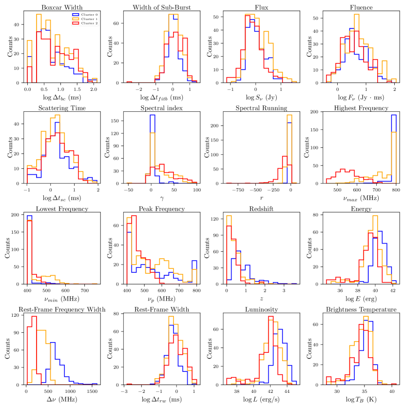
Figure 4: The distributions of 16 parameters across different clusters from k-means are illustrated, with blue, orange, and red histogram step lines representing Cluster 0, Cluster 1, and Cluster 2, respectively.

To improve the clustering results, we optimize the hyperparameters of the clustering algorithm by maximizing the mean silhouette coefficient  (Rousseeuw, 1987) across all samples. The silhouette coefficient measures how well a sample fits within its assigned cluster, with values ranging from -1 to 1. Higher values indicate more tightly grouped, well-defined clusters. We show the mean silhouette coefficients changed with the hyperparameters of the clustering algorithm in Figure 2. In this work, we chose the hyperparameters with max mean silhouette coefficients, which is n_clusters = 3 for k-means, min_cluster_size = 37  and min_samples = 3 for HDBSCAN.

3.2 Evaluation Metrics

In this study, we experimented with various machine learning algorithms and hyperparameters, and their classification performance requires evaluation using specific metrics. The outputs of clustering can be written as the following forms:

• $TP$: The true positives, which means the number of repeaters correctly classified in the repeater cluster.

• $TN$: The true negatives, represent the number of non-repeaters correctly classified in the non-repeater cluster.

• $FP$: The false positives, represent the number of non-repeaters incorrectly classified in the repeater cluster.

• $FN$: The false negatives, indicating the number of repeaters incorrectly classified into the non-repeater cluster.

Generally, based on the four outputs mentioned above, various metrics can be calculated to evaluate the model’s performance:

• Recall: ${TP}/{(TP+FN)}$.

• Precision: ${TP}/{(TP+FP)}$.

• Accuracy: ${(TP+TN)}/{(TP+TN+FP+FN)}$.

In this study, we use recall to evaluate the model’s performance, as observational limitations prevent the accurate determination of non-repeaters, making it impossible to reliably estimate $TN$ and $FP$.

4 Results and Discussion

4.1 Dimensionality reduction and clustering

Based on the methods and hyperparameters discussed in Section 3.1.1, we present the UMAP-dimensionally reduced features of 745 FRBs in the left panel of Figure 3. The blue dots represent non-repeaters, while the green and red crosses indicate repeaters from Cat1 and Cat2023, respectively. It is evident that after dimensionality reduction by UMAP, the repeaters are clustered in the upper right corner, while a distinct group of pure non-repeaters appears in the lower left corner, separated by a noticeable gap from the mixture. This indicates that the 16 parameters of FRBs used in the analysis have the ability to distinguish between non-repeaters and repeaters.

Then we used two types of clustering algorithm, k-means and HDBSCAN, to cluster the two-dimensional UMAP embedding. We present the clustering results in the middle and right panels of Figure 3, based on the hyperparameters of k-means and HDBSCAN discussed in Section 3.1.2. If the proportion of repeaters in a cluster exceeds 30%, we classify it as a “ repeater cluster ”, with the non-repeaters within it considered as “ repeater candidates ”. Conversely, if the proportion is below 30%, it is classified as an “ non-repeater cluster ”.

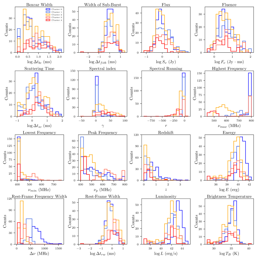
Figure 5: Same as Figure 4, but displays the results from HDBSCAN. The blue, royal blue, orange, tomato, and red histogram step lines represent Cluster 0, 1, 2, 3, and 4, respectively.

As shown in the middle panel of Figure 3, the k-means algorithm divided the UMAP-embedded data into three clusters. Cluster 0 contains 210 FRBs, all of which are non-repeaters. Cluster 2 consists of 294 FRBs, including 98 repeaters and 196 repeater candidates (the percentage of repeaters is 33.3%). Cluster 3 contains 235 FRBs, with 132 repeaters (the percentage of repeaters is 56.2%) and 103 repeater candidates. All repeaters are classified into repeater clusters, giving a recall of 100%. Out of the 509 non-repeaters, 299 repeater candidates were identified (from 269 non-repeater sources). If these repeater candidates are real, the repeating rate of FRBs would reach approximately 61.7%, exceeding the predicted rates from studies such as Chen et al. (2022), Zhu-Ge et al. (2022), and Yang et al. (2023).

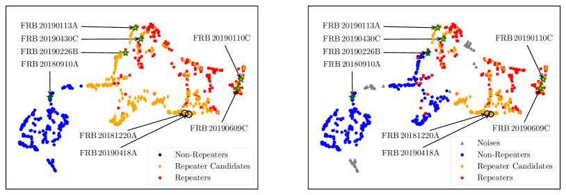
Figure 6: The distribution of non-repeaters (blue dots), repeater candidates (orange diamonds), and repeaters (red crosses) is presented in the clustered UMAP-embedded data from both k-means (left panel) and HDBSCAN (right panel). And the gray triangles are represent noises. The green stars mark the first bursts of six repeaters that were misidentified as non-repeaters. The black circles indicate the localized non-repeaters.

As shown in the right panel of Figure 3, HDBSCAN divided the UMAP-embedded data into five clusters and a noise cluster. Cluster 0 contains 169 FRBs, all of which are non-repeaters. Cluster 1 includes 15 repeaters and 138 non-repeaters, with repeaters making up only 9.8%. Clusters 2, 3, and 4 contain 206, 94, and 58 FRBs, with 88, 66, and 47 repeaters (repeaters accounting for 42. 7%, 70. 2%, and 81. 0%, respectively) and repeater candidates numbering 118, 28, and 11 (a total of 157 candidates, corresponding to 141 non-repeater sources). The recall for the 739 samples is 93.1%. The overall repeating rate is around 37.9%, slightly lower than the results of Yamasaki et al. (2023); McGregor & Lorimer (2024), but comparable to those of Chen et al. (2022), Zhu-Ge et al. (2022), and Yang et al. (2023). Detailed clustering results for both algorithms are also presented in Table 1.

We plot the feature distributions of different clusters generated by k-means and HDBSCAN in Figure 4 and Figure 5, respectively. As shown in Figure 4, the rest-frame frequency width differs the most across clusters, indicating that repeater clusters tend to have narrower frequency bandwidths. Significant differences are also observed in the distributions of the spectral index, highest frequency, redshift, energy, luminosity, and brightness temperature among the clusters. These results are consistent with the feature distribution of repeaters and non-repeaters shown in Figure 1. In Figure 5, almost all features show notable differences in their distributions between clusters, with rest-frame frequency width once again being the most distinct, similar to the results in Figure 4.

As mentioned in Section 2, there are 6 FRB sources that were previously observed as non-repeaters in Cat1 but were later identified as repeaters in Cat2023. We marked these 6 FRBs in Figure 6 with green open stars to analyze the reliability of our repeater candidate predictions. The left and right panels of Figure 6 show the repeater candidate predictions from k-means and HDBSCAN, respectively. For k-means, five out of these 6 FRB sources are located in the repeater clusters and were successfully identified as repeater candidates, while HDBSCAN predicted four of them successfully. This indicates that our method is effective in identifying potential repeaters. However, one of these 6 FRBs stands out—FRB 20180910A—which was classified into the non-repeater cluster by both clustering algorithms. After analyzing its 16 parameters, we found that its boxcar width is only 0.98 ms, and its spectral index (0.05) and spectral running (-0.53) are very similar to those of non-repeaters. Additionally, its broadband emission characteristics differ significantly from the narrow-band emission typically observed in repeaters. Currently, there is no satisfactory theoretical explanation for repeaters that exhibit characteristics so similar to non-repeaters. We also found that FRB 20180910A has so far produced three detected bursts, with intervals of 1 year and 9 months. These bursts exhibit noticeable differences in boxcar width, bandwidth, spectral index, and spectral running. It is possible that these bursts are from different non-repeaters within the same galaxy (or neighboring galaxies in the same direction). Further observations are needed to confirm this.

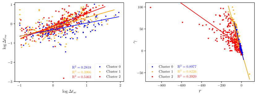
Figure 7: The empirical relationships between scattering time (${\rm log\,}\Delta t_{sc}$) and rest-frame width (${\rm log\,}\Delta t_{rw}$) (left panel), and between spectral acceleration ($r$) and spectral index ($\gamma$) (right panel) are shown for FRBs in different clusters from k-means, represented by blue, orange, and red lines, respectively. The corresponding $R^{2}$ values (in blue, orange, and red) are also provided. See Section 4.2 for details.

x	y	cluster	$a$	$b$	$R^{2}$
${\rm log\,}\Delta t_{sc}$	${\rm log\,}\Delta t_{rw}$	0	0.3440	-0.3055	0.2818
		1	0.4954	-0.1744	0.3966
		2	0.6572	-0.1256	0.5463
$r$	$\gamma$	0	-0.9000	-1.6846	0.8977
		1	-0.7853	-1.9914	0.8226
		2	-0.1613	11.4422	0.3920

Table 2: The slope ($a$), intercept ($b$), and $R^{2}$ values of the empirical relations for different clusters from k-means.

Additionally, some of the non-repeaters from Cat1 have identified host galaxies (Bhardwaj et al., 2024; Law et al., 2020). In both panels of Figure 6, we highlight two of these FRBs (FRB 20181220A and FRB 20190418A) that were identified as repeater candidates by both clustering algorithms with black circles. Continued observations of the host galaxies of these two FRBs may reveal further repeating bursts in the future.

4.2 Empirical Relationships

In this paper, we further analyze the potential two-dimensional empirical relations within different clusters identified by various clustering algorithms. We pair the 16 parameters of FRBs from different clusters and linearly fit the data points using scipy.stats.linregress , which performs linear least-squares regression. The form of the two-dimensional empirical relationship is given as $y=a\,x+b$, and the goodness of fit is evaluated using the score (coefficient of determination), defined as $R^{2}=1-\sum_{i}(y_{i}-\hat{y}_{i})^{2}/\sum{i}(y_{i}-\bar{y}_{i})^{2}$, where $y_{i}$, $\hat{y}_{i}$, and $\bar{y}_{i}$ are the observed values, the regressed values and the mean of the observed values, respectively. The closer $R^{2}$ is to 1, the better the model fits the data.

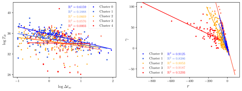
Figure 8: The empirical relationships between scattering time (${\rm log\,}\Delta t_{sc}$) and brightness temperature (${\rm log\,}T_{B}$) (left panel), and between spectral acceleration ($r$) and spectral index ($\gamma$) (right panel) are shown for FRBs in different clusters from HDBSCAN, represented by blue, royal blue, orange, tomato, and red lines, respectively. The corresponding $R^{2}$ values (in blue, royal blue, orange, tomato, and red) are also provided. See Section 4.2 for details.

x	y	cluster	$a$	$b$	$R^{2}$
${\rm log\,}\Delta t_{sc}$	${\rm log\,}T_{B}$	0	-1.4741	35.8475	0.6159
		1	-1.0264	34.9418	0.1888
		2	-0.7559	34.4684	0.0669
		3	-0.9667	34.4318	0.0576
		4	-0.098	34.1223	0.0003
$r$	$\gamma$	0	-0.9394	-2.2495	0.9125
		1	-0.6574	-2.6236	0.8386
		2	-0.4835	-7.4780	0.8053
		3	-0.8527	4.4482	0.9187
		4	-0.1090	11.8615	0.5293

Table 3: The slope ($a$), intercept ($b$), and $R^{2}$ values of the empirical relations for different clusters from HDBSCAN.

We set a high score threshold of $R^{2}>0.5$ to filter out well-fitted empirical relations and excluded parameter combinations that inherently have a linear relationship (e.g., luminosity and flux). For the clusters from k-means, the selected empirical relations are shown in Figure 7, and the slope, intercept, and score of the empirical relations are listed in Table 2. The left panel shows the empirical relation between two independent parameters: scattering time (${\rm log\,}\Delta t_{sc}$) and rest-frame width (${\rm log\,}\Delta t_{rw}$). We observe that $R^{2}>0.5$ only in cluster 2, corresponding to a repeater cluster, whereas the ${\rm log\,}\Delta t_{sc}-{\rm log\,}\Delta t_{rw}$ relation appears less significant in the other two clusters. However, the slope and intercept of the relation ${\rm log\,}\Delta t_{sc}-{\rm log\,}\Delta t_{rw}$ are similar in all three clusters. The right panel displays the empirical relation between two other independent parameters: spectral acceleration ($r$) and spectral index ($\gamma$). In contrast to the ${\rm log\,}\Delta t_{rw}-{\rm log\,}\Delta t_{sc}$ relation, the $r-\gamma$ relation is less evident in cluster 2, but is very pronounced in clusters 0 and 1 ($R^{2}>0.8$), with similar slopes and intercepts.

Figure 8 shows the empirical relations for different clusters from HDBSCAN, and Table 3 lists the slope, intercept, and score of these empirical relations. The left panel displays the relation between rest-frame width (${\rm log\,}\Delta t_{sc}$) and the brightness temperature (${\rm log\,}T_{B}$), which are also two independent parameters. We can see that only cluster 0 (a non-repeater cluster) has a significant ${\rm log\,}\Delta t_{sc}-{\rm log\,}T_{B}$ relation with $R^{2}>0.6$, while the other clusters show no strong ${\rm log\,}\Delta t_{sc}-{\rm log\,}T_{B}$ relation. The right panel shows the empirical relation between spectral acceleration ($r$) and spectral index ($\gamma$). All clusters exhibit a significant $r-\gamma$ relation, especially clusters 0-3, where $R^{2}>0.8$. Notably, clusters 0 and 3 (a repeater cluster) have very similar slopes and intercepts for the $r-\gamma$ relation, suggesting that certain repeaters might have spectral properties similar to those of non-repeaters, a trend also observed in the k-means results..

5 Conclusion and Future Prospect

Machine learning is a powerful tool to classify FRBs. In this paper, we applied unsupervised learning methods, including dimensionality reduction and clustering algorithms, to differentiate between repeaters and non-repeaters in the first CHIME/FRB catalog (CHIME/FRB Collaboration et al., 2021) and the CHIME/FRB Collaboration (2023) catalog (CHIME/FRB Collaboration et al., 2023). We extracted 16 parameters from the FRBs to serve as input features for unsupervised learning, ensuring that the information from the FRBs was sufficiently comprehensive. Ultimately, we successfully identified several candidate repeaters among the non-repeaters. Using the UMAP+k-means method, we identified 269 non-repeaters as repeater candidates, with an estimated repeating rate of 61.7%. With the UMAP+HDBSCAN method, 141 non-repeaters were identified as repeater candidates, yielding a repeating rate of 37.9%. Additionally, we found that FRBs in repeater clusters and non-repeater clusters exhibit different distributions across several features, suggesting that repeaters and non-repeaters may belong to distinct categories.

We used six previously classified as non-repeaters but actually confirmed as repeaters FRB sources to evaluate the predictive capability of our model. The UMAP + k-means method successfully predicted five of these sources, while the UMAP + HDNSCAN method successfully predicted four. The only exception was FRB 20180910A, which could not be predicted. The reason for this is that many of its characteristics, such as frequency bandwidth, spectral index, and spectral running, closely resemble those of non-repeaters, making it distinctly different from typical repeaters. Additionally, the intervals between the three outbursts of this repeater are quite long, and the features of each burst show significant variation. This may indicate that the FRB sources are unrelated and originate from different galaxies within the same direction or from the same galaxy. Furthermore, within Cat1, there are some localized non-repeaters, and we identified two of them as repeater candidates using both clustering algorithms. Continued observations of the host galaxies of these two FRBs may reveal additional repeating bursts in the future.

We further analyzed the empirical relations that may exist within different clusters. For the clusters derived from k-means, we identified a significant ${\rm log\,}\Delta t_{sc}-{\rm log\,}\Delta t_{rw}$ relation exclusive to cluster 2, as well as a $r-\gamma$ relation present only in clusters 0 and 1. For the clusters obtained through HDBSCAN, we found a notable ${\rm log\,}\Delta t_{sc}-{\rm log\,}T_{B}$ relation that exists solely in cluster 0, along with the $r-\gamma$ relation observed across all clusters. The spectral index $\gamma$ and spectral running $r$ are the shape parameters of FRB spectrum, described by a continuous power-law function (Pleunis et al., 2021; Planck Collaboration et al., 2020):

$$I(\nu)=A(\nu/\nu_{0})^{\gamma+r\,{\rm ln}(\nu/\nu_{0})},$$ (8)

where $I(\nu)$ is the intensity at spectral frequency $\nu$, A is the amplitude, and $\nu_{0}$ is the pivotal frequency, set at 400.1953125 MHz, the lower limit of the CHIME band. The strict $r-\gamma$ relation means that only one parameter can determine the morphology of FRB. We also noted that the $r-\gamma$ relation is similar in certain clusters of both non-repeaters and repeaters, such as clusters 0 and 1 from k-means and clusters 0 and 3 from HDBSCAN. This suggests that some non-repeaters and repeaters share comparable spectral characteristics. This finding aligns with observational evidence, particularly regarding FRB 20180910A, if it is indeed a genuine repeater.

In the future, improvements in observational data and machine learning techniques will refine FRB classification, reduce misclassifications, and uncover more repeaters. The use of advanced clustering algorithms and multi-wavelength observations will enhance the accuracy of models, while deep learning approaches may reveal new patterns. These advancements will contribute to a better understanding of the origins and physical mechanisms of FRBs, with potential implications for cosmology.

References

- Adámek & Armour (2020) Adámek, K., & Armour, W. 2020, ApJS, 247, 56, doi: 10.3847/1538-4365/ab7994
- Agarwal et al. (2020) Agarwal, D., Aggarwal, K., Burke-Spolaor, S., Lorimer, D. R., & Garver-Daniels, N. 2020, MNRAS, 497, 1661, doi: 10.1093/mnras/staa1856
- Andersen et al. (2020) Andersen, B. C., et al. 2020, Nature, 587, 54, doi: 10.1038/s41586-020-2863-y
- Bhardwaj et al. (2024) Bhardwaj, M., Michilli, D., Kirichenko, A. Y., et al. 2024, ApJ, 971, L51, doi: 10.3847/2041-8213/ad64d1
- Bhatporia et al. (2023) Bhatporia, S., Walters, A., Murugan, J., & Weltman, A. 2023, arXiv e-prints, arXiv:2311.03456, doi: 10.48550/arXiv.2311.03456
- Bochenek et al. (2020) Bochenek, C. D., Ravi, V., Belov, K. V., et al. 2020, Nature, 587, 59, doi: 10.1038/s41586-020-2872-x
- Breiman (2001) Breiman, L. 2001, Machine Learning, 45, 5, doi: 10.1023/A:1010933404324
- Burke-Spolaor & Bannister (2014) Burke-Spolaor, S., & Bannister, K. W. 2014, Astrophys. J., 792, 19, doi: 10.1088/0004-637X/792/1/19
- Campello et al. (2013) Campello, R. J. G. B., Moulavi, D., & Sander, J. 2013, in Advances in Knowledge Discovery and Data Mining, ed. J. Pei, V. S. Tseng, L. Cao, H. Motoda, & G. Xu (Berlin, Heidelberg: Springer Berlin Heidelberg), 160–172
- Campello et al. (2015) Campello, R. J. G. B., Moulavi, D., Zimek, A., & Sander, J. 2015, ACM Trans. Knowl. Discov. Data, 10, doi: 10.1145/2733381
- Chang & Lin (2011) Chang, C.-C., & Lin, C.-J. 2011, ACM Trans. Intell. Syst. Technol., 2, doi: 10.1145/1961189.1961199
- Chen et al. (2021) Chen, B. H., Hashimoto, T., Goto, T., et al. 2021, Mon. Not. Roy. Astron. Soc., 509, 1227, doi: 10.1093/mnras/stab2994
- Chen et al. (2022) Chen, B. H., Hashimoto, T., Goto, T., et al. 2022, MNRAS, 509, 1227, doi: 10.1093/mnras/stab2994
- Chen et al. (2023) Chen, B. H., Hashimoto, T., Goto, T., et al. 2023, Mon. Not. Roy. Astron. Soc., 521, 5738, doi: 10.1093/mnras/stad930
- CHIME/FRB Collaboration et al. (2018) CHIME/FRB Collaboration, Amiri, M., Bandura, K., et al. 2018, ApJ, 863, 48, doi: 10.3847/1538-4357/aad188
- CHIME/FRB Collaboration et al. (2021) CHIME/FRB Collaboration, Amiri, M., Andersen, B. C., et al. 2021, ApJS, 257, 59, doi: 10.3847/1538-4365/ac33ab
- CHIME/FRB Collaboration et al. (2023) CHIME/FRB Collaboration, Andersen, B. C., Bandura, K., et al. 2023, ApJ, 947, 83, doi: 10.3847/1538-4357/acc6c1
- Cordes & Lazio (2002) Cordes, J. M., & Lazio, T. J. W. 2002, arXiv e-prints, astro, doi: 10.48550/arXiv.astro-ph/0207156
- Cover & Hart (1967) Cover, T., & Hart, P. 1967, IEEE Trans. Inf. Theor., 13, 21–27, doi: 10.1109/TIT.1967.1053964
- Dempster et al. (2018) Dempster, A. P., Laird, N. M., & Rubin, D. B. 2018, Journal of the Royal Statistical Society: Series B (Methodological), 39, 1, doi: 10.1111/j.2517-6161.1977.tb01600.x
- Deng & Zhang (2014) Deng, W., & Zhang, B. 2014, Astrophys. J. Lett., 783, L35, doi: 10.1088/2041-8205/783/2/L35
- Ester et al. (1996) Ester, M., Kriegel, H.-P., Sander, J., Xu, X., et al. 1996in , 226–231
- Fonseca et al. (2020) Fonseca, E., et al. 2020, Astrophys. J. Lett., 891, L6, doi: 10.3847/2041-8213/ab7208
- Fotopoulou (2024) Fotopoulou, S. 2024, Astronomy and Computing, 48, 100851, doi: 10.1016/j.ascom.2024.100851
- Gao et al. (2014) Gao, H., Li, Z., & Zhang, B. 2014, Astrophys. J., 788, 189, doi: 10.1088/0004-637X/788/2/189
- Gordon et al. (2023) Gordon, A. C., Fong, W.-f., Kilpatrick, C. D., et al. 2023, ApJ, 954, 80, doi: 10.3847/1538-4357/ace5aa
- Guo & Wei (2022) Guo, H.-Y., & Wei, H. 2022, JCAP, 07, 010, doi: 10.1088/1475-7516/2022/07/010
- Guo & Wei (2024) —. 2024, Phys. Lett. B, 859, 139120, doi: 10.1016/j.physletb.2024.139120
- Hallinan et al. (2019) Hallinan, G., et al. 2019. https://arxiv.org/abs/1907.07648
- Han et al. (2012) Han, J., Kamber, M., & Pei, J. 2012, in Data Mining (Third Edition), third edition edn., ed. J. Han, M. Kamber, & J. Pei, The Morgan Kaufmann Series in Data Management Systems (Boston: Morgan Kaufmann), 443–495, doi: https://doi.org/10.1016/B978-0-12-381479-1.00010-1
- J. et al. (2019) J., K., et al. 2019, Mon. Not. Roy. Astron. Soc., 489, 919, doi: 10.1093/mnras/stz2219
- Jankowski et al. (2023) Jankowski, F., et al. 2023, Mon. Not. Roy. Astron. Soc., 524, 4275, doi: 10.1093/mnras/stad2041
- Keane (2018) Keane, E. F. 2018, Nature Astron., 2, 865, doi: 10.1038/s41550-018-0603-0
- Kirsten et al. (2022) Kirsten, F., et al. 2022, Nature, 602, 585, doi: 10.1038/s41586-021-04354-w
- Kumar & Zhang (2014) Kumar, P., & Zhang, B. 2014, Phys. Rept., 561, 1, doi: 10.1016/j.physrep.2014.09.008
- Kumar et al. (2019) Kumar, P., Shannon, R. M., Osłowski, S., et al. 2019, ApJ, 887, L30, doi: 10.3847/2041-8213/ab5b08
- Law et al. (2020) Law, C. J., Butler, B. J., Prochaska, J. X., et al. 2020, ApJ, 899, 161, doi: 10.3847/1538-4357/aba4ac
- Law et al. (2024) Law, C. J., et al. 2024, Astrophys. J., 967, 29, doi: 10.3847/1538-4357/ad3736
- Li et al. (2021a) Li, C. K., et al. 2021a, Nature Astron., 5, 378, doi: 10.1038/s41550-021-01302-6
- Li & Pan (2016) Li, D., & Pan, Z. 2016, Radio Science, 51, 1060, doi: 10.1002/2015RS005877
- Li et al. (2024) Li, L.-Y., Jia, J.-Y., Qiang, D.-C., & Wei, H. 2024, arXiv e-prints, arXiv:2408.12983, doi: 10.48550/arXiv.2408.12983
- Li et al. (2021b) Li, X. J., Dong, X. F., Zhang, Z. B., & Li, D. 2021b, Astrophys. J., 923, 230, doi: 10.3847/1538-4357/ac3085
- Li et al. (2019) Li, Z., Gao, H., Wei, J.-J., et al. 2019, Astrophys. J., 876, 146, doi: 10.3847/1538-4357/ab18fe
- Lin et al. (2020) Lin, L., et al. 2020, Nature, 587, 63, doi: 10.1038/s41586-020-2839-y
- Lloyd (1982) Lloyd, S. 1982, IEEE transactions on information theory, 28, 129
- Lorimer (2018) Lorimer, D. R. 2018, Nature Astron., 2, 860, doi: 10.1038/s41550-018-0607-9
- Lorimer et al. (2007) Lorimer, D. R., Bailes, M., McLaughlin, M. A., Narkevic, D. J., & Crawford, F. 2007, Science, 318, 777, doi: 10.1126/science.1147532
- Luo et al. (2022) Luo, J.-W., Zhu-Ge, J.-M., & Zhang, B. 2022, Mon. Not. Roy. Astron. Soc., 518, 1629, doi: 10.1093/mnras/stac3206
- MacQueen et al. (1967) MacQueen, J., et al. 1967in , Oakland, CA, USA, 281–297
- McGregor & Lorimer (2024) McGregor, K., & Lorimer, D. R. 2024, Astrophys. J., 961, 10, doi: 10.3847/1538-4357/ad1184
- McInnes et al. (2017) McInnes, L., Healy, J., & Astels, S. 2017, Journal of Open Source Software, 2, 205, doi: 10.21105/joss.00205
- McInnes et al. (2018) McInnes, L., Healy, J., & Melville, J. 2018. https://arxiv.org/abs/1802.03426
- Niu et al. (2022) Niu, C. H., et al. 2022, Nature, 606, 873, doi: 10.1038/s41586-022-04755-5
- Petroff et al. (2022) Petroff, E., Hessels, J. W. T., & Lorimer, D. R. 2022, Astron. Astrophys. Rev., 30, 2, doi: 10.1007/s00159-022-00139-w
- Petroff et al. (2015) Petroff, E., et al. 2015, Mon. Not. Roy. Astron. Soc., 451, 3933, doi: 10.1093/mnras/stv1242
- Petroff et al. (2016) Petroff, E., Barr, E. D., Jameson, A., et al. 2016, Publ. Astron. Soc. Austral., 33, e045, doi: 10.1017/pasa.2016.35
- Planck Collaboration et al. (2020) Planck Collaboration, Aghanim, N., Akrami, Y., et al. 2020, A&A, 641, A6, doi: 10.1051/0004-6361/201833910
- Pleunis et al. (2021) Pleunis, Z., Good, D. C., Kaspi, V. M., et al. 2021, ApJ, 923, 1, doi: 10.3847/1538-4357/ac33ac
- Qiang et al. (2020) Qiang, D.-C., Deng, H.-K., & Wei, H. 2020, Class. Quant. Grav., 37, 185022, doi: 10.1088/1361-6382/ab7f8e
- Qiang et al. (2022) Qiang, D.-C., Li, S.-L., & Wei, H. 2022, JCAP, 01, 040, doi: 10.1088/1475-7516/2022/01/040
- Qiang & Wei (2020) Qiang, D.-C., & Wei, H. 2020, JCAP, 04, 023, doi: 10.1088/1475-7516/2020/04/023
- Qiang & Wei (2021) —. 2021, Phys. Rev. D, 103, 083536, doi: 10.1103/PhysRevD.103.083536
- Raquel et al. (2023) Raquel, B. J. R., Hashimoto, T., Goto, T., et al. 2023, Mon. Not. Roy. Astron. Soc., 524, 1668, doi: 10.1093/mnras/stad1942
- Ravi (2019) Ravi, V. 2019, Nature Astron., 3, 928, doi: 10.1038/s41550-019-0831-y
- Ravi & Lasky (2014) Ravi, V., & Lasky, P. D. 2014, Mon. Not. Roy. Astron. Soc., 441, 2433, doi: 10.1093/mnras/stu720
- Rousseeuw (1987) Rousseeuw, P. J. 1987, Journal of Computational and Applied Mathematics, 20, 53, doi: https://doi.org/10.1016/0377-0427(87)90125-7
- Rumelhart et al. (1986) Rumelhart, D. E., Hinton, G. E., & Williams, R. J. 1986, Nature, 323, 533, doi: 10.1038/323533a0
- Shannon et al. (2024) Shannon, R. M., Bannister, K. W., Bera, A., et al. 2024, arXiv e-prints, arXiv:2408.02083, doi: 10.48550/arXiv.2408.02083
- Sharma et al. (2024) Sharma, K., et al. 2024. https://arxiv.org/abs/2409.16964
- Spitler et al. (2014) Spitler, L. G., et al. 2014, Astrophys. J., 790, 101, doi: 10.1088/0004-637X/790/2/101
- Spitler et al. (2016) —. 2016, Nature, 531, 202, doi: 10.1038/nature17168
- Sun et al. (2024) Sun, W.-P., Zhang, J.-G., Li, Y., et al. 2024. https://arxiv.org/abs/2409.11173
- Thornton et al. (2013) Thornton, D., et al. 2013, Science, 341, 53, doi: 10.1126/science.1236789
- Vapnik (1999) Vapnik, V. 1999, IEEE Transactions on Neural Networks, 10, 988, doi: 10.1109/72.788640
- Wagstaff et al. (2016) Wagstaff, K. L., Tang, B., Thompson, D. R., et al. 2016, PASP, 128, 084503, doi: 10.1088/1538-3873/128/966/084503
- Wang & Wei (2023) Wang, B., & Wei, J.-J. 2023, Astrophys. J., 944, 50, doi: 10.3847/1538-4357/acb2c8
- Wang et al. (2020a) Wang, F. Y., Wang, Y. Y., Yang, Y.-P., et al. 2020a, Astrophys. J., 891, 72, doi: 10.3847/1538-4357/ab74d0
- Wang & Zhang (2019) Wang, F. Y., & Zhang, G. Q. 2019, Astrophys. J., 882, 108, doi: 10.3847/1538-4357/ab35dc
- Wang et al. (2020b) Wang, W.-Y., Xu, R., & Chen, X. 2020b, Astrophys. J., 899, 109, doi: 10.3847/1538-4357/aba268
- Wei et al. (2019) Wei, J.-J., Li, Z., Gao, H., & Wu, X.-F. 2019, JCAP, 09, 039, doi: 10.1088/1475-7516/2019/09/039
- Wu et al. (2019) Wu, D., Cao, H., Lv, N., et al. 2019, ApJ, 887, L10, doi: 10.3847/2041-8213/ab595e
- Xiao & Dai (2022) Xiao, D., & Dai, Z.-G. 2022, Astron. Astrophys., 657, L7, doi: 10.1051/0004-6361/202142268
- Xiao et al. (2021) Xiao, D., Wang, F., & Dai, Z. 2021, Sci. China Phys. Mech. Astron., 64, 249501, doi: 10.1007/s11433-020-1661-7
- Xiao et al. (2022) —. 2022, Fast Radio Bursts, ed. C. Bambi & A. Santangelo (Singapore: Springer Nature Singapore), 1–38, doi: 10.1007/978-981-16-4544-0_128-1
- Xu et al. (2022) Xu, H., Niu, J. R., Chen, P., et al. 2022, Nature, 609, 685, doi: 10.1038/s41586-022-05071-8
- Xu et al. (2023) Xu, J., et al. 2023, Universe, 9, 330, doi: 10.3390/universe9070330
- Yamasaki et al. (2023) Yamasaki, S., Goto, T., Ling, C.-T., & Hashimoto, T. 2023, Mon. Not. Roy. Astron. Soc., 527, 11158, doi: 10.1093/mnras/stad3844
- Yang et al. (2023) Yang, X., Zhang, S. B., Wang, J. S., & Wu, X. F. 2023, Mon. Not. Roy. Astron. Soc., 522, 4342, doi: 10.1093/mnras/stad1304
- Yang et al. (2021) Yang, X., Zhang, S. B., Wang, J. S., et al. 2021, MNRAS, 507, 3238, doi: 10.1093/mnras/stab2275
- Yang et al. (2017) Yang, Y.-P., Luo, R., Li, Z., & Zhang, B. 2017, Astrophys. J. Lett., 839, L25, doi: 10.3847/2041-8213/aa6c2e
- Yang & Zhang (2016) Yang, Y.-P., & Zhang, B. 2016, Astrophys. J. Lett., 830, L31, doi: 10.3847/2041-8205/830/2/L31
- Zhang (2014) Zhang, B. 2014, Astrophys. J. Lett., 780, L21, doi: 10.1088/2041-8205/780/2/L21
- Zhang et al. (2007) Zhang, B., Zhang, B.-B., Liang, E.-W., et al. 2007, Astrophys. J. Lett., 655, L25, doi: 10.1086/511781
- Zhang & Li (2018) Zhang, M.-J., & Li, H. 2018, Eur. Phys. J. C, 78, 460, doi: 10.1140/epjc/s10052-018-5953-3
- Zhang & Zhang (2022) Zhang, R. C., & Zhang, B. 2022, Astrophys. J. Lett., 924, L14, doi: 10.3847/2041-8213/ac46ad
- Zhang et al. (2021) Zhang, R. C., Zhang, B., Li, Y., & Lorimer, D. R. 2021, Mon. Not. Roy. Astron. Soc., 501, 157, doi: 10.1093/mnras/staa3537
- Zhang et al. (2018) Zhang, Y. G., Gajjar, V., Foster, G., et al. 2018, ApJ, 866, 149, doi: 10.3847/1538-4357/aadf31
- Zhou et al. (2014) Zhou, B., Li, X., Wang, T., Fan, Y.-Z., & Wei, D.-M. 2014, Phys. Rev. D, 89, 107303, doi: 10.1103/PhysRevD.89.107303
- Zhu-Ge et al. (2022) Zhu-Ge, J.-M., Luo, J.-W., & Zhang, B. 2022, Mon. Not. Roy. Astron. Soc., 519, 1823, doi: 10.1093/mnras/stac3599
- Zhu-Ge et al. (2023) Zhu-Ge, J.-M., Luo, J.-W., & Zhang, B. 2023, MNRAS, 519, 1823, doi: 10.1093/mnras/stac3599