22institutetext: Universität Tübingen, Tübingen, Germany
33institutetext: National Technical University of Athens, Greece 44institutetext: Universität Würzburg, Würzburg, Germany
Minimum Monotone Spanning Trees††thanks: This work was initiated at the GNV Workshop 2022 at Heiligkreuztal.
Abstract
Computing a Euclidean minimum spanning tree of a set of points is a seminal problem in computational geometry and geometric graph theory. We combine it with another classical problem in graph drawing, namely computing a monotone geometric representation of a given graph. More formally, given a finite set of points in the plane and a finite set of directions, a geometric spanning tree with vertex set is -monotone if, for every pair of vertices of , there exists a direction for which the unique path from to in is monotone with respect to . We provide a characterization of -monotone spanning trees. Based on it, we show that a -monotone spanning tree of minimum length can be computed in polynomial time if the number of directions is fixed, both when (i) the set of directions is prescribed and when (ii) the objective is to find a minimum-length -monotone spanning tree over all sets of directions. For , we describe algorithms that are much faster than those for the general case. Furthermore, in contrast to the classical Euclidean minimum spanning tree, whose vertex degree is at most six, we show that for every even integer , there exists a point set and a set of directions such that any minimum-length -monotone spanning tree of has maximum vertex degree .
1 Introduction
We study a problem that combines the notion of minimum spanning tree of a set of points in the plane with the notion of monotone drawings of graphs.
The problem of computing a (Euclidean) minimum spanning tree (MST) of a set of points in the plane is a well-established topic with a long history in computational geometry [27]. An MST of a finite set of points is a geometric tree such that: spans , i.e., the vertices of are the points of , and has minimum length subject to property , where the length of is the sum of the lengths of its edges and the length of an edge is the Euclidean distance of its endpoints. Equivalently, the MST is the minimum spanning tree of the complete graph on where the weight of each edge is the Euclidean distance of its incident vertices. It is known that an MST is a subgraph of a Delaunay triangulation [49] (see Figs. 1(a) and 1(b)). Given a set of points, its Delaunay triangulation has at most edges, hence an MST of can be computed in time (in the real RAM model of computation) via standard MST algorithms. Eppstein [19] has a survey on MSTs.
Monotone drawings of graphs have been introduced by the authors of [4] and have received considerable attention in recent years. They are related to other types of drawings of graphs, such as angle-monotone [10, 11, 12, 15, 36], upward [17, 24], greedy [3, 6, 15, 16, 45, 47], self-approaching [1, 9, 42], and increasing-chord drawings [8, 15, 39, 42]. Computing monotone drawings is also related to the geometric problem of finding monotone trajectories between two given points in the plane avoiding convex obstacles [7]. A plane path is monotone with respect to a direction if the order of its vertices along the path coincides with the order of their projections on a line parallel to . Any monotone path is necessarily crossing-free [4]. A straight-line drawing of a graph in the plane is monotone if there exists a monotone path (with respect to some direction) between any two vertices of ; the direction of monotonicity may be different for each path. If the directions of monotonicity for the paths are restricted to a set of directions, then the drawing is -monotone. Results about monotone drawings include algorithms for different graph classes [2, 4, 5, 20] and the study of the area requirement of such drawings (see [30, 33, 43] for monotone drawings of trees and [31, 32, 44] for different classes of planar graphs).


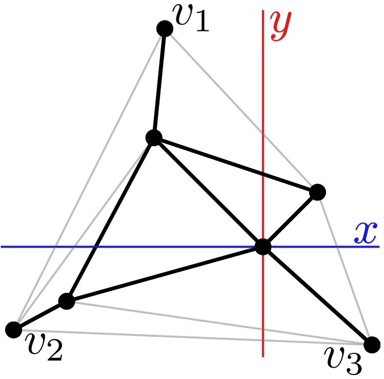
Our setting. In this paper, we study a natural setting that combines the benefits of spanning trees of minimum length with the benefits of monotone drawings. Namely, given a set of points in the plane and a prescribed set of directions, we study the problem of computing a -monotone spanning tree of of minimum length (see Fig. 1(c)). We call such a tree a minimum -monotone spanning tree. For a point set and an integer , we also address the problem of computing a minimum -directional monotone spanning tree of , i.e., a -monotone spanning tree of minimum length among all possible sets of directions. In this variant, the choice of the directions of monotonicity adjusts to the given point set, which can lead to shorter monotone spanning trees.
We remark that there are other prominent attempts in the literature to couple the MST problem with an additional property. For example, the Euclidean degree- MST asks for an MST whose maximum degree is bounded by a given integer [21, 46]. Seo, Lee, and Lin [48] studied MSTs of smallest diameter or smallest radius. Finding the smallest spanning trees [18, 22, 23] or dynamic MSTs [14, 50] are further problems related to spanning trees.
Particularly relevant to our study is the Rooted Monotone MST problem introduced by Mastakas and Symvonis [40] and further studied by Mastakas [38]. In that problem, given a set of points with a designated root , the task is to compute an MST such that the path from to any other point of is monotone. Mastakas [37] extended this setting to multiple roots.
Contribution. The main results in this paper are as follows:
- •
-
•
Regarding , we describe - and -time algorithms for and , respectively. For , we present an XP-algorithm that runs in time; see LABEL:se:k-monotone\arxivlncs{ and LABEL:se:appendix-mmst-s-k}{}.
- •
The proofs of statements with a (clickable) “” appear in the appendix.
2 Basic Definitions
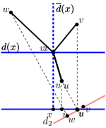
Let denote the unit circle centered at the origin of . Any segment oriented from the center of to a point of defines a direction vector or simply a direction. Two directions are opposite if the two segments that define them belong to the same line and lie on opposite sides of the origin. Given a direction and a set of points in the plane, we say that is in -general position if no two points in lie on a line orthogonal to . If is in -general position, let be the linear ordering of the orthogonal projections of the points of on any line parallel to and directed as ; note that is uniquely defined. Given a direction and a point set in -general position, we say that the geometric path is -monotone if or ; in this case, all projections of the oriented segments (for on a line parallel to point towards the same direction. A path is monotone if it is -monotone with respect to some direction .
Let be a finite set of points, and let be a finite set of directions such that no two of them are opposite. A spanning tree of is -monotone if, for every pair of vertices of , there is a such that the unique geometric path from to in is -monotone (which requires that the subset of points on the path from to is in -general position).
A minimum -monotone spanning tree of is a -monotone spanning tree of of minimum length among all -monotone spanning trees of ; we call the problem of computing such a tree. For a positive integer , we say that a spanning tree of is -directional monotone if there exists a set of directions such that is -monotone. A minimum -directional monotone spanning tree of is a -directional monotone spanning tree of of minimum length among all -directional monotone spanning trees of ; we call the problem of computing such a tree. To solve this problem, it turns out that it is sufficient to consider only sets of directions such that is in -general position, i.e., is in -general position for every .
Given two points and , let be the line passing through and . Given a direction and a point , let be the line parallel to passing through and let be the direction orthogonal to obtained by rotating counterclockwise (ccw.) by an angle of . Accordingly, is the line orthogonal to and is the line orthogonal to passing through . Given two vertices and of a geometric tree , let denote the path of from to .
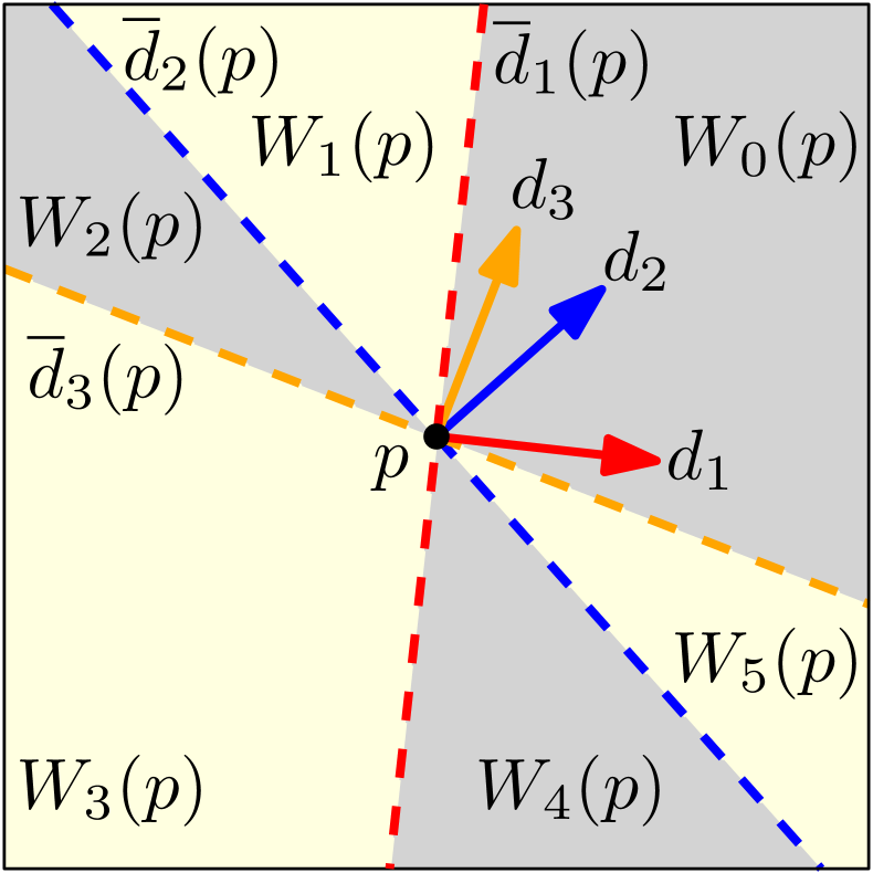
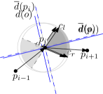
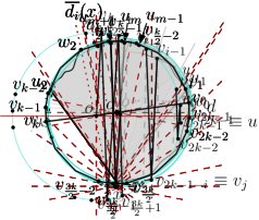
Given a sorted set of pairwise non-opposite directions (assumed to be sorted with respect to the directions’ slopes) and a point in the plane, let be the set of wedges determined by the lines . See Fig. 2 on page 2 for an illustration where . We fix the numbering of the wedges by starting with an arbitrary wedge and then continue with in ccw. order around . Whenever we refer to a wedge for some integer , we assume that is taken modulo . If coincides with the origin , we just write instead of .
For a directed geometric path and , let be the oriented segment starting from the origin that is parallel to and has the same orientation as . Define , the sector of directions of path , to be the smallest sector of the unit circle that includes the oriented segment for every ; see Figs. 3(a) and 3(b).


Moreover, let be the wedge set of the directed path , i.e., the smallest set of consecutive wedges in counterclockwise (ccw.) order whose union contains ; see Fig. 3(c). For a point , let be the region of the plane determined by translated such that is its apex. If is the reverse path of , then consists of the wedges opposite to those in . We say that path utilizes wedge set .
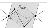
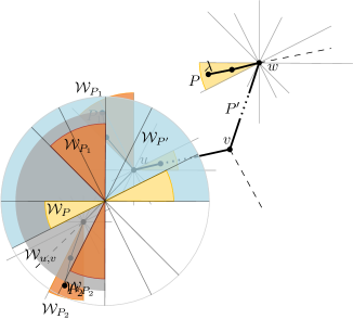
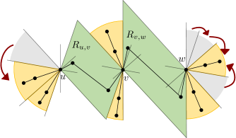
In a -monotone spanning tree , a branching vertex is a vertex of degree at least 3 and a leaf path is a path of degree-2 vertices from a branching vertex to a leaf. Given two adjacent branching vertices and in , the branch is the unique path that connects and via a sequence of degree-2 vertices. Both a leaf path and a branch may consist of a single edge. Further, for any pair of (not necessarily adjacent) vertices and , let be the subtree of consisting of and all subtrees hanging from except for the one containing . Let , the wedge set of , be the smallest set of consecutive wedges that contains all wedges utilized by either leaf paths or branches oriented away from in and that does not contain the wedge utilized by the edge out of that leads to vertex ; see Fig. 4. Note that if and/or is a leaf, then and/or . Let be the region defined by the wedges in translated such that is their apex.

3 Properties of Monotone Paths and Trees
We describe basic properties of monotone paths and -monotone trees, which we use in Section 4. Unless otherwise stated, we assume that consists of pairwise non-opposite directions and that the point set is always in -general position.
Lemma 1 (\IfAppendix)
Let be a set of points, and let be a geometric path on . Let be a direction such that is in -general position. If and lie in the same half-plane determined by , then the path is not -monotone.
The next lemma generalizes Lemma 1. It concerns the wedges formed by a set of directions (in contrast to the half-plane formed by the perpendicular to a single direction) and two arbitrary points in the same wedge.
Lemma 2 (\IfAppendix)
Let be a set of points, let be a spanning tree of , and let be a set of directions. Let , , and be points in such that . If and lie in the same wedge in , then the path is not -monotone.
For any vertex of , the set of lines partitions the plane into wedges with apex , each wedge containing at most one neighbor of .
Lemma 3 (\IfAppendix)
Let be a set of points, let be a set of directions, and let be a -monotone spanning tree of . Let denote the maximum degree of tree . Then, .
The authors of [4] gave the following characterization.
Lemma 4 ([4])
Let be a directed geometric path. Then, is monotone if and only if the angle of its sector of directions is smaller than .
While Lemma 4 can be used to recognize monotone paths, it does not specify a direction of monotonicity. This is rectified by Lemma 5.
Lemma 5 (\IfAppendix)
Given a direction , a monotone directed geometric path is -monotone if and only if does not intersect , where is the origin.
The following corollary is an immediate consequence of Lemma 5.
Corollary 1
Let be a set of points, be a set of directions, and be a -monotone spanning tree of . Let be a directed path in . Given a direction , is -monotone if and only if does not intersect the interior of , where is the origin.
Additional properties concerning paths of -monotone spanning trees and their corresponding wedge sets are presented in the following lemma.
Lemma 6 (\IfAppendix)
Let be a set of points, let be a set of directions, and let be a -monotone spanning tree of . Then, has the following properties: (i) Let be a directed path originating at vertex of . Then, lies in . (ii) Let and be two edge-disjoint directed paths originating at internal vertices and of and terminating at leaves of . Then, sets and are disjoint and regions and are disjoint.
Lemma 6 immediately implies the next bound on the number of leaves of -monotone trees.
Lemma 7
Let be a set of points, and let be a set of directions. If is a -monotone spanning tree of , then has at most leaves.
The following lemma generalizes Lemma 6 (which concerns paths) for subtrees of a -monotone spanning tree .
Lemma 8 (\IfAppendix)
Let be a set of points, let be a set of directions, let be a -monotone spanning tree of , and let and be two vertices of . Then, it holds that: (i) Subtree of lies in . (ii) Sets and are disjoint, and regions and are disjoint.
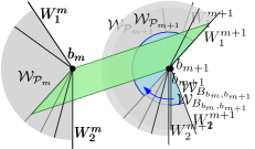
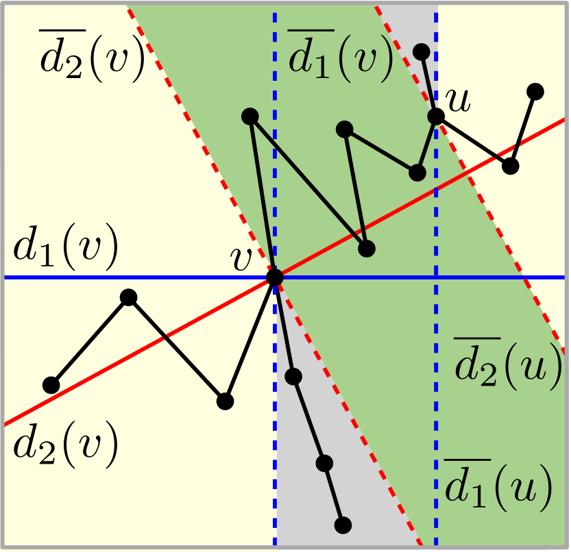
Let be a branch of a -monotone tree connecting branching vertices and . Recall that , due to monotonicity of . Let . If , then is a parallelogram; see Fig. 5(a). Otherwise (i.e., if ), is a strip bounded by the parallel lines and , where is the direction of monotonicity of ; see Fig. 5(b). We call the region of branch . Similarly, if is a leaf path from to , then we define the region of the leaf path .

4 A Characterization of -Monotone Spanning Trees
In this section we provide a characterization of -monotone spanning trees. It is the basis for our algorithm that solves ; see Section 5.
Theorem 4.1
Let be a set of points, let be a set of (pairwise non-opposite) directions such that is in -general position, and let be a spanning tree of . Then, is -monotone if and only if:
-
(a)
Every leaf path and every branch in is -monotone.
-
(b)
For every two leaf paths and incident to branching vertices and , respectively, and are disjoint.
-
(c)
For every branch or leaf path of it holds that .
Proof
Since is a -monotone tree, any subtree of is also -monotone and, hence statement (a) holds. Statement (b) follows from Lemma 6(ii) since any two leaf paths are edge-disjoint. Statement (c) follows from Lemma 9.
For the monotonicity of , it suffices to show that, for any two leaves and , the path is -monotone. Let and be the leaf paths to and where and are the branching vertices they are incident to, respectively. Suppose first that and are incident to the same vertex, i.e., . Due to (a), both leaf paths are -monotone; hence, and . Also, due to (b), and are disjoint. Hence, there exists a direction in such that separates and and does not intersect the interior of either of them. By Corollary 1, and are both -monotone and, additionally, they lie in different halfplanes with respect to . Hence, the path from to is -monotone, and thus -monotone.
Suppose now that . Let be the sequence of the branching vertices on in order of appearance where, for convenience, is treated as a branching vertex. By Corollary 1, it suffices to show that there is a direction such that does not intersect the interior of . Let denote the subpath of from vertex to leaf . We show by induction on the size of that for every , . Since is by definition the oriented path from to , the fact that together with Corollary 1 guarantee that there exists a direction such that the path from to is -monotone. For the base of the induction, observe that is the leaf path , which is -monotone by (a). For the induction hypothesis, assume that for . We show that . Assume, for a contradiction, that . Since consists of and of the branch , the wedges of are due to branch . Let and be the leading and the trailing wedges (in ccw. order) of and let and be the leading and the trailing wedges (in ccw. order) of . Observe first that either or . If this was not the case, then which contradicts the fact that all branches are -monotone (refer to Fig. 6(a)).

Now assume, w.l.o.g., that (see Fig. 6(b)). The leading wedge of is , and the branch uses at most wedges as it is -monotone. Also, contains vertex as otherwise it would not be -monotone. Consider now the utilized wedge set of consisting of the opposite of . Its leading wedge is the opposite of , it is located before (in ccw. order), and its trailing wedge is located after (in ccw. order). Thus, intersects the region of the branch (the green parallelogram in Fig. 6(b)). This is a contradiction, as due to (c). Note that considering as a branching vertex does not affect the correctness of the proof. ∎
5 Algorithms for
In this section we prove that the problem is in XP with respect to , that is, it can be solved in polynomial time for any fixed value of . An embedding of a tree is prescribed by the clockwise circular order of the edges incident to each vertex of the tree. A tree with a given embedding is an embedded tree. A homeomorphically irreducible tree (HIT), is an embedded tree without vertices of degree two [28]. Let and be two trees; we say that and have the same topology if they are (possibly different) subdivisions of the same HIT . Two trees with the same topology have the same embedding if the circular order of the edges around the vertices is the same in both trees. Given a HIT and any embedded tree that is a subdivision of , we say that corresponds to . Since for a vertex of degree two the circular order of its incident edges is unique, the embedding of a tree uniquely defines the embedding of the corresponding HIT. Note that, given an embedded tree and the corresponding HIT , an internal vertex of corresponds to a branching vertex of , a leaf of to a leaf path of , and an edge between two internal vertices of to a branch of .
Let be the numbers of HITs with at most leaves. We can use a result of Harary, Robinson, and Schwenk [29] concerning the number of (non-embedded) trees with vertices to derive a bound for . However, this does not yield an algorithm to generate all different HITs with at most leaves. For this reason we give an upper bound that is based on a generation scheme. Note that our scheme may generate the same HIT several times.
Lemma 10 (\IfAppendix)
The number of different HITs with at most leaves is , and these HITs can be enumerated in time.
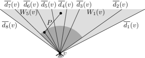
We now present an overview of the algorithm for solving the problem. It examines every HIT with at most leaves. Since there are many (-monotone) spanning trees that are subdivisions of the same HIT, the algorithm examines for each HIT all of its -monotone spanning trees on . Let be the HIT under consideration, and let and be the numbers of leaves and branching vertices of , respectively. Let be one of the possible mappings of the branching vertices to points in . Let be an assignment of the wedges of to the leaves of so that each leaf receives a distinct set of consecutive wedges. Assigning (as part of ) the set of consecutive wedges to a leaf incident to a branching vertex of can be interpreted as our intention to cover all points in region by the monotone leaf path that ends at . As shown in Fig. 7, the monotone leaf path may utilize a set of consecutive wedges , i.e., some of the leading and/or trailing wedges of may not be utilized by .
The point set , the set of (pairwise non-opposite) directions, the HIT , together with mapping and assignment , form an instance of a restricted problem that asks for a minimum -monotone spanning tree having as its HIT and respecting and . Let denote this problem instance. Note that such a monotone spanning tree may not exist. If it exists, it turns out that it is unique (see Lemma 11). The algorithm for solving instances of type is repeatedly used by the algorithm that proves Theorem 5.1.
Lemma 11 (\IfAppendix)
Let be a set of points, let be a set of (pairwise non-opposite) directions, let be a HIT, let be a mapping of the internal vertices of to points of , and let be an assignment of to the leaves of so that each leaf receives a distinct set of consecutive wedges. Then, can be solved in time. Moreover, if a solution to the exists, then it is unique.
Proof
Based on the characterization in Theorem 4.1, the algorithm checks whether point set admits a -monotone spanning tree whose associated HIT is , respecting mapping and assignment . Condition (b) of Theorem 4.1 is satisfied by definition since is a valid assignment. For condition (c), we first compute the set that consists of all path regions and branch regions and for every branch , we compute and . These computations take time since HIT has size . Then, the algorithm verifies, for every edge of , whether regions and are disjoint, in time. For condition (a), we compute, for every remaining point in , the region of that contains , in time. We then check, for every region in , whether there exists a path that (i) is monotone with respect to the two directions that are orthogonal to its boundaries and (ii) spans all points in the region. This can be done in time by sorting the points according to both directions. If the spanning tree exists, its uniqueness follows from the fact that each region in contains a unique -monotone path. ∎
Theorem 5.1 (\IfAppendix)
Let be a set of points, and let be a set of (pairwise non-opposite) distinct directions. There exists a function such that, if is in -general position, then we can compute a minimum -monotone spanning tree of in time. In other words, the problem is in XP when parameterized by .
Proof
The given set of directions yields a set of wedges. Hence, a -monotone spanning tree has at most leaves and at most branching vertices. We enumerate the at most HITs according to Lemma 10. Let be the current HIT, let be the number of leaves, and let be the number of branching vertices of . We go through each of the subsets of cardinality of . Let be the mapping of the branching vertices of to points in . Let be the assignment of a set of consecutive wedges in to the leaves of . There are at most many such assignments since we have choices for mapping the first leaf to some wedge, and then we select out of the remaining wedges that we attribute to a different leaf than the preceding wedge (in circular order). For each of the , (with ) choices of a HIT , mapping and assignment , we run the algorithm presented in the proof of Lemma 11 for the , which terminates in time. Finally, we return the shortest tree that we have found (if any). The total runtime is , where . We argue the correctness of the algorithm in Appendix 0.B. ∎
Speed-Up for : For , the algorithm from Section 5 computes a -monotone spanning tree of a set of points in the plane in time. In Section 0.B.1, we show how to speed this up to time.
Solving : When the set of directions is not prescribed and we are asked to search over all possible sets of directions, a minimum -directional monotone spanning tree of a point set can be identified in and in time for and , respectively. For , we describe an XP algorithm that runs in time w.r.t. ; see Appendix 0.C.
6 Maximum Degree of the Minimum -Directional MST
Since the (Euclidean) MST has maximum degree at most six [25], it is natural to ask whether this upper bound carries over to minimum -directional monotone spanning trees. We prove that this is not the case by presenting a set of specific directions and a set of points such that the unique monotone -directional spanning tree of has degree .
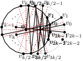
Let be an even positive integer, and let be the set of distinct (pairwise non-opposite) directions (in ccw. order) such that is defined by the vector and, for , . Since is even, it holds that where . For simplicity, we consider to be the wedge defined by and . We define to be the set of points, where is the origin and, for , is placed on the unit circle in the (ccw.) second angle-trisection of wedge of ; see Fig. 8(a). By construction is the vertex set of a regular -gon centered at and the star with edges is a valid monotone spanning tree for of length . Thus, any solution of has length at most .
Let be a tree that spans . We call polygon vertices the vertices of distinct from . We refer to edges of connecting adjacent polygon vertices as external, to edges incident to as rays and to all other edges as chords.


To show that the unique solution to the instance is the -star centered at , we first establish that polygon vertices have degree at most 2.
Proof
Let tree be a solution to the instance and assume that is not the -star with at its center. It is easy to show that a leaf of cannot be the endpoint of a chord. By using this property together with the fact that all polygon vertices of have degree at most 2 (Lemma 12), we can show that must contain the path , (Fig. 8(b)). Consider the tree formed by replacing the edges of by rays from to the path vertices. Clearly, is also monotone. To show that is not optimal, it suffices to show that the length of is greater than the total length of the rays that replaced the edges of in or, equivalently, that . Indeed, using geometry, we show that . ∎
7 Open Problems
We have presented an XP algorithm for solving . It is natural to ask whether this problem is NP-hard if is part of the input (rather than a fixed constant).
Another research direction is to study, for a given point set and a set of directions, the problem of computing a minimum -monotone spanning graph for . Note that such a graph can have much smaller total length than a solution to . Indeed, Theorem 6.1 shows that there is a point set (Fig. 8(a)) and a set of directions such that the only solution to is the -star, which has a total length of . A monotone spanning graph of (see Fig. 8(c)) has a total length of at most .
References
- [1] Soroush Alamdari, Timothy M. Chan, Elyot Grant, Anna Lubiw, and Vinayak Pathak. Self-approaching graphs. In Walter Didimo and Maurizio Patrignani, editors, Proc. 20th Int. Symp. Graph Drawing (GD’12), volume 7704 of LNCS, pages 260–271. Springer, 2012. doi:10.1007/978-3-642-36763-2\_23.
- [2] Patrizio Angelini. Monotone drawings of graphs with few directions. Inform. Process. Lett., 120:16–22, 2017. doi:10.1016/j.ipl.2016.12.004.
- [3] Patrizio Angelini, Michael A. Bekos, Walter Didimo, Luca Grilli, Philipp Kindermann, Tamara Mchedlidze, Roman Prutkin, Antonios Symvonis, and Alessandra Tappini. Greedy rectilinear drawings. Theor. Comput. Sci., 795:375–397, 2019. doi:10.1016/J.TCS.2019.07.019.
- [4] Patrizio Angelini, Enrico Colasante, Giuseppe Di Battista, Fabrizio Frati, and Maurizio Patrignani. Monotone drawings of graphs. J. Graph Algorithms Appl., 16(1):5–35, 2012. doi:10.7155/jgaa.00249.
- [5] Patrizio Angelini, Walter Didimo, Stephen Kobourov, Tamara Mchedlidze, Vincenzo Roselli, Antonios Symvonis, and Stephen Wismath. Monotone drawings of graphs with fixed embedding. Algorithmica, 71:233–257, 2015. doi:10.1007/s00453-013-9790-3.
- [6] Patrizio Angelini, Fabrizio Frati, and Luca Grilli. An algorithm to construct greedy drawings of triangulations. J. Graph Algorithms Appl., 14(1):19–51, 2010. doi:10.7155/jgaa.00197.
- [7] Esther M. Arkin, Robert Connelly, and Joseph S. B. Mitchell. On monotone paths among obstacles with applications to planning assemblies. In Proc. 5th Ann. ACM Symp. Comput. Geom. (SoCG), pages 334–343, 1989. doi:10.1145/73833.73870.
- [8] Yeganeh Bahoo, Stephane Durocher, Sahar Mehrpour, and Debajyoti Mondal. Exploring increasing-chord paths and trees. In Joachim Gudmundsson and Michiel Smid, editors, Proc. 29th Canadian Conf. Comput. Geometry (CCCG), pages 19–24, 2017.
- [9] Davood Bakhshesh and Mohammad Farshi. (Weakly) Self-approaching geometric graphs and spanners. Comput. Geom., 78:20–36, 2019. doi:10.1016/j.comgeo.2018.10.002.
- [10] Davood Bakhshesh and Mohammad Farshi. Angle-monotonicity of Delaunay triangulation. Comput. Geom., 94:101711, 2021. doi:10.1016/j.comgeo.2020.101711.
- [11] Davood Bakhshesh and Mohammad Farshi. On the plane angle-monotone graphs. Comput. Geom., 100:101818, 2022. doi:10.1016/j.comgeo.2021.101818.
- [12] Nicolas Bonichon, Prosenjit Bose, Paz Carmi, Irina Kostitsyna, Anna Lubiw, and Sander Verdonschot. Gabriel triangulations and angle-monotone graphs: Local routing and recognition. In Yifan Hu and Martin Nöllenburg, editors, Proc. Int. Symp Graph Drawing & Network Vis. (GD), volume 9801 of LNCS, pages 519–531. Springer, 2016. doi:10.1007/978-3-319-50106-2_40.
- [13] Bernard Chazelle and David P. Dobkin. Intersection of convex objects in two and three dimensions. J. ACM, 34(1):1–27, 1987. doi:10.1145/7531.24036.
- [14] Francis Chin and David Houck. Algorithms for updating minimal spanning trees. J. Comput. Syst. Sci., 16(3):333–344, 1978. doi:10.1016/0022-0000(78)90022-3.
- [15] Hooman Reisi Dehkordi, Fabrizio Frati, and Joachim Gudmundsson. Increasing-chord graphs on point sets. In Christian Duncan and Antonios Symvonis, editors, Proc. Int. Symp. Graph Drawing (GD), volume 8871 of LNCS, pages 464–475. Springer, 2014. doi:10.1007/978-3-662-45803-7_39.
- [16] Raghavan Dhandapani. Greedy drawings of triangulations. Discrete. Comput. Geom., 43:375–392, 2010. doi:10.1007/s00454-009-9235-6.
- [17] Walter Didimo. Upward graph drawing. In Ming-Yang Kao, editor, Encyclopedia of Algorithms, pages 2308–2312. Springer, 2016. doi:10.1007/978-1-4939-2864-4\_653.
- [18] David Eppstein. Finding the smallest spanning trees. BIT, 32:237–248, 1992. doi:10.1007/BF01994879.
- [19] David Eppstein. Spanning trees and spanners. In J.-R. Sack and J. Urrutia, editors, Handbook of Computational Geometry, pages 425–461. North-Holland, Amsterdam, 2000. doi:10.1016/B978-044482537-7/50010-3.
- [20] Stefan Felsner, Alexander Igamberdiev, Philipp Kindermann, Boris Klemz, Tamara Mchedlidze, and Manfred Scheucher. Strongly monotone drawings of planar graphs. In Sándor Fekete and Anna Lubiw, editors, Proc. 32nd Int. Symp. Comput. Geom. (SoCG), volume 51 of LIPIcs, pages 37:1–37:15. Schloss Dagstuhl – Leibniz-Zentrum für Informatik, 2016. doi:10.4230/LIPIcs.SoCG.2016.37.
- [21] Andrea Francke and Michael Hoffmann. The Euclidean degree-4 minimum spanning tree problem is NP-hard. In Proc. 25th Ann. ACM Symp. Comput. Geom. (SoCG), pages 179–188, 2009. doi:10.1145/1542362.1542399.
- [22] Greg N. Frederickson. Ambivalent data structures for dynamic 2-edge-connectivity and smallest spanning trees. SIAM J. Comput., 26(2):484–538, 1997. doi:10.1137/S0097539792226825.
- [23] Harold N. Gabow. Two algorithms for generating weighted spanning trees in order. SIAM J. Comput., 6:139–150, 1977. doi:10.1137/0206011.
- [24] Ashim Garg and Roberto Tamassia. Upward planarity testing. Order, 12(2):109–133, 1995. doi:10.1007/BF01108622.
- [25] George Georgakopoulos and Christos H. Papadimitriou. The 1-Steiner tree problem. J. Algorithms, 8(1):122–130, 1987. doi:10.1016/0196-6774(87)90032-0.
- [26] Jacob E. Goodman and Richard Pollack. On the combinatorial classification of nondegenerate configurations in the plane. J. Combin. Theory Ser. A, 29(2):220–235, 1980. doi:10.1016/0097-3165(80)90011-4.
- [27] Ronald L. Graham and Pavol Hell. On the history of the minimum spanning tree problem. Ann. Hist. Comput., 7(1):43–57, 1985. doi:10.1109/MAHC.1985.10011.
- [28] Frank Harary and Geert Prins. The number of homeomorphically irreducible trees, and other species. Acta Math., 101(1–2):141–162, 1959. doi:10.1007/BF02559543.
- [29] Frank Harary, Robert W. Robinson, and Allen J. Schwenk. Twenty-step algorithm for determining the asymptotic number of trees of various species. J. Austral. Math. Soc., 20(4):483–503, 1975. doi:10.1017/S1446788700016190.
- [30] Dayu He and Xin He. Optimal monotone drawings of trees. SIAM J. Discrete Math., 31(3):1867–1877, 2017. doi:10.1137/16M1080045.
- [31] Xin He and Dayu He. Monotone drawings of 3-connected plane graphs. In Nikhil Bansal and Irene Finocchi, editors, Proc. Europ. Symp. Algorithms (ESA), volume 9294 of LNCS, pages 729–741. Springer, 2015. doi:10.1007/978-3-662-48350-3_61.
- [32] Md. Iqbal Hossain and Md. Saidur Rahman. Good spanning trees in graph drawing. Theoret. Comput. Sci., 607:149–165, 2015. doi:10.1016/j.tcs.2015.09.004.
- [33] Philipp Kindermann, André Schulz, Joachim Spoerhase, and Alexander Wolff. On monotone drawings of trees. In Christian Duncan and Antonios Symvonis, editors, Proc. Int. Symp. Graph Drawing (GD), volume 8871 of LNCS, pages 488–500. Springer, 2014. doi:10.1007/978-3-662-45803-7_41.
- [34] Michael P. Knapp. Sines and cosines of angles in arithmetic progression. Mathematics Magazine, 82(5):371–372, 2009. doi:10.4169/002557009X478436.
- [35] Hsiang-Tsung Kung, Fabrizio L. Luccio, and Franco P. Preparata. On finding the maxima of a set of vectors. J. ACM, 22(4):469–476, 1975. doi:10.1145/321906.321910.
- [36] Anna Lubiw and Debajyoti Mondal. Construction and local routing for angle-monotone graphs. J. Graph Algorithms Appl., 23(2):345–369, 2019. doi:10.7155/jgaa.00494.
- [37] Konstantinos Mastakas. Uniform 2d-monotone minimum spanning graphs. In Stephane Durocher and Shahin Kamali, editors, Proc 30th Canadian Conf. Comput. Geom. (CCCG), pages 318–325, 2018. URL: https://arxiv.org/abs/1806.08770.
- [38] Konstantinos Mastakas. Drawing a rooted tree as a rooted -monotone minimum spanning tree. Inform. Process. Lett., 166:106035, 2021. doi:10.1016/j.ipl.2020.106035.
- [39] Konstantinos Mastakas and Antonios Symvonis. On the construction of increasing-chord graphs on convex point sets. In Proc. 6th Int. Conf. Inform. Intell. Syst. Appl. (IISA), pages 1–6, 2015. doi:10.1109/IISA.2015.7388028.
- [40] Konstantinos Mastakas and Antonios Symvonis. Rooted uniform monotone minimum spanning trees. In Dimitris Fotakis, Aris Pagourtzis, and Vangelis Th. Paschos, editors, Proc. Int. Conf. Algorithms & Complexity (CIAC), volume 10236 of LNCS, pages 405–417. Springer, 2017. doi:10.1007/978-3-319-57586-5_34.
- [41] Dragoslav S. Mitrinović. Analytic Inequalities. Springer, 1970. doi:10.1007/978-3-642-99970-3.
- [42] Martin Nöllenburg, Roman Prutkin, and Ignaz Rutter. On self-approaching and increasing-chord drawings of 3-connected planar graphs. J. Comput. Geom., 7(1):47–69, 2016. doi:10.20382/jocg.v7i1a3.
- [43] Anargyros Oikonomou and Antonios Symvonis. Simple compact monotone tree drawings. In Fabrizio Frati and Kwan-Liu Ma, editors, Proc. 25th Int. Symp. Graph Drawing & Netw. Vis. (GD), volume 10692 of LNCS, pages 326–333. Springer, 2017. doi:10.1007/978-3-319-73915-1_26.
- [44] Anargyros Oikonomou and Antonios Symvonis. Monotone drawings of -inner planar graphs. In Therese Biedl and Andreas Kerren, editors, Proc. 26th Int. Symp. Graph Drawing & Netw. Vis. (GD), volume 11282 of LNCS, pages 347–353. Springer, 2018. doi:10.1007/978-3-030-04414-5_24.
- [45] Christos H. Papadimitriou and David Ratajczak. On a conjecture related to geometric routing. Theor. Comput. Sci., 344(1):3–14, 2005. doi:10.1016/j.tcs.2005.06.022.
- [46] Christos H. Papadimitriou and Umesh V. Vazirani. On two geometric problems related to the travelling salesman problem. J. Algorithms, 5(2):231–246, 1984. doi:10.1016/0196-6774(84)90029-4.
- [47] Ananth Rao, Sylvia Ratnasamy, Christos Papadimitriou, Scott Shenker, and Ion Stoica. Geographic routing without location information. In Proc. 9th Ann. ACM Conf. Mobile Comput. Network. (MobiCom), pages 96–108, 2003. doi:10.1145/938985.938996.
- [48] Dae Young Seo, Der-Tsai Lee, and Tien-Ching Lin. Geometric minimum diameter minimum cost spanning tree problem. In Proc. 20th Int. Symp. Algorithms & Comput. (ISAAC), page 283–292. Springer, 2009. doi:10.1007/978-3-642-10631-6\_30.
- [49] Michael Ian Shamos and Dan Hoey. Closest-point problems. In Proc. 16th Ann. IEEE Symp. Foundat. Comput. Sci. (FOCS), pages 151–162, 1975. doi:10.1109/SFCS.1975.8.
- [50] P. M. Spira and A. Pan. On finding and updating spanning trees and shortest paths. SIAM J. Comput., 4(3):375–380, 1975. doi:10.1137/0204032.
Appendix 0.A Additional Material for Section 3
See 1
Proof
It is immediate to see that in the linear ordering , the projection of either precedes or follows both the projections of and . Hence, the path is not -monotone (see Fig. 9). ∎
See 2
Proof
Let . For the path to be monotone with respect to some direction , it must hold that and are located in different half-planes of so that appears between and in . This is not possible, however, since and lie in the same wedge in . ∎
See 3
Proof
Let be an arbitrary vertex of . The set of lines partitions the plane into wedges with apex . By Lemma 1, if two neighbors and of lie in the same wedge, then they lie in the same halfplane with respect to every direction in . Hence, the path is not monotone with respect to any direction in . Since is -monotone, it follows that no two neighbors of lie in the same wedge with apex , which implies that . ∎
See 5
Proof
Assume first that is -monotone. Suppose by contradiction that intersects ; refer to Fig. 10(a). Let and , and , be the oriented segments of the unit circle that delimit the sector of directions . Then, the projections of the oriented segments and on line point in opposite directions. This is a clear contradiction since all the projections of the oriented segments , , of a monotone path point in the same direction. Also, note that in the boundary case where overlaps with or (or both), path cannot be monotone since the projections of at least two of its points on coincide; another contradiction.
Assume now that does not intersect . Consider three consecutive path points , , and let the unit circle be centered at point ; refer to Fig. 10(b). As points and are on opposite sides of line , the projections of the oriented segments and on line point in the same direction. Thus, path is monotone. ∎

See 6
Proof
(i) Let and be the two directions in orthogonal to the boundaries of . Then, due to Corollary 1, path is both - and -monotone. Let be the vertex incident to on . Then, by definition of we have that lies in . Now let, for the sake of contradiction, be a vertex of that lies outside the region . Observe that vertices and lie in the same halfplane with respect either to or . Therefore, due to Lemma 1, path is not monotone with respect to both and . A contradiction.
(ii) Let and where and are internal vertices of and and are the corresponding leaves. Since and are edge-disjoint, path from to is composed of , and . Since is -monotone, must be -monotone with respect to at least one direction, say . It follows that for any internal vertex in the path the oriented subpaths and lie in different halfplanes with respect to .
-
(a)
For the sake of contradiction assume that and overlap. Then, for we get that all vertices of must lie behind . At the same time, for we get that all vertices of path must lie ahead of . However, due to the fact that and overlap, no such direction exists; a contradiction to the monotonicity of path .
-
(b)
As shown in (a), subpaths and lie in different halfplanes with respect to (or ). Given that and are disjoint, we conclude that .
∎
See 8
Proof
(i) Consider first a path from vertex oriented towards an arbitrary leaf of . By Lemma 6(i), we have that path lies in region . Since path is composed of branches (zero or more) and a single leaf path in it follows that and, in turn, that path lies in region . Since the union of all paths from to the leaves of covers all branches and leaf paths in is follows that lies in .
(ii) Observe that if one of the vertices or , say , is a leaf, then . Therefore, both statements of the lemma trivially hold. The same applies if and are distinct leaves. So, in the remainder of the proof we assume that and are internal tree vertices.
-
(a)
For the sake of contradiction assume that and overlap. By Lemma 6(ii), we know that there do not exist directed paths and terminating at leaves of that belong in and , respectively, such that overlaps with . So, without loss of generality, we assume that there exists a path originating at an internal vertex in and terminating at leaf in such that . Furthermore, let and be the paths terminating at leaves of utilizing the leading and trailing wedges of , respectively. Refer to Fig. 11. Since is an embedded monotone tree, so is its subtree that consists of and the path from to (which passes from and ) and uses the same embedding as . Consider path from to and let be its first edge. Then, is a path terminating at leaf and its set of utilized wedges includes the wedge utilized by edge , the wedges in and the wedges in . Thus, path is, at least, utilizing all wedges also utilized by either or . Without loss of generality, assume that intersects with . However, given that both and are edge-disjoint paths terminating at leaves, by Lemma 6(ii), we have that and are disjoint, a clear contradiction. We conclude that and are disjoint.
-
(b)
Recall that due to (a) we have that and are disjoint. By the definition of and it follows that the leading and the trailing wedges of and are utilized. Let and be the leading and the trailing wedges of and let and be the leading and the trailing wedges of in ccw. order. Assume for the sake of contradiction that areas and intersect. Then, at least one of intersects with at least one of . W.l.o.g., let intersect with and let be the oriented edge away of that utilizes wedge and be the oriented edge away of that utilizes wedge . Let be the path of originating at that utilizes wedge and let be the path of originating at that utilizes wedge . Since is an embedded -monotone tree, so is its subtree that uses the same embedding. But, in , paths and are edge-disjoint and terminate at leaves of . Due to Lemma 6(ii), regions and are disjoint. A contradiction.
∎

See 9
Proof
Let be the subtree of formed by and . Tree is -monotone since it is a subtree of . Consider first the case where consists only of edge . Then, by definition, edge utilizes a wedge which is not contained in and, thus, it immediately follows that . Consider now the case where path contains at least one intermediate vertex. Let be the edge of incident to . Edge utilizes a wedge which is not contained in . Consider now vertices and of and subtrees and . By Lemma 8(ii) we have that and are disjoint with respect to and, therefore, they are also disjoint with respect to . Since and is composed of edge and , we conclude that .
Now, observe that . Since regions and have the same apex and are contained in the disjoint sets of utilized wedges and , respectively, we also conclude that . ∎
Appendix 0.B Additional Material for Section 5
See 10
Proof
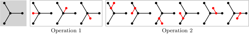
Denote by the number of different HITs with exactly leaves, for . We now prove, by induction on , that for . For there exists only one possible HIT, i.e., the tree consisting of a single edge. Suppose that . A HIT with leaves can be obtained from a HIT with leaves by means of one of two operations: by attaching an edge (and a leaf) to an internal vertex (we call this Operation 1) or by subdividing an edge and attaching a new edge to the degree-two vertex created by the subdivision (we call this Operation 2). See Fig. 12 for an illustration.
Let be an HIT with leaves. Given , let be the set of vertices, let be the set of internal vertices, let be the set of leaves, and let be the number of edges of . If we perform Operation 1 on an internal vertex of the tree , we can obtain different HITs, which have the same topology but different embedding depending on the position of the new edge in the circular order around . Thus, the number of different HITs that can be generated starting from by performing Operation 1 is . We have . The term is equal to the number of leaves, that is ; moreover, since the number of leaves is , the number of vertices is at most , and the number of edges is at most . Thus, we obtain . If we perform Operation 2 on an edge of , we can obtain different HITs depending on the side of where the new edge is added. Thus, from the tree we can obtain at most different HITs, which implies . By induction, and therefore .
The number of different HITs with at most leaves can now be computed as . Clearly, all these HITs can be generated starting from the single tree with two leaves as described above by performing Operations 1 and 2. Since each operation can be executed in time, the whole set can be generated in time. ∎
See 11
Proof
Let be the internal vertices of . As discussed, every internal vertex of corresponds to a branching vertex in the solution of the problem . For each branch of we compute and based on assignment . This computation can be easily completed in total time. Since and are complementary, the candidate region is uniquely defined. The same holds for and . Let be the set of points in that correspond to internal vertices of through mapping . For each branch with , our algorithm checks whether region is a valid area of the plane by verifying that lies in . If is valid, then must be contained in it; otherwise, the algorithm rejects the tuple .
The assignment of the wedges of to the leaves of defines, for each leaf path, a reagion that must contain it. Let denote the set of all leaf path regions and branch regions (that have already been computed). Observe that .
Due to Theorem 4.1, if is either a branch or a leaf path of a -monotone spanning tree, then areas and must be disjoint. Since is bounded by two semi-lines originating at and is either a parallelogram or a strip between two parallel lines the test for their intersection can be completed in constant time [13]. In total, we can check in time all intersections suggested by Theorem 4.1.
Now we compute, in total time, for each point in , the region in that contains . Due to Lemma 6(i) every leaf path incident to a branching vertex in the solution of the should be contained in and every branch between two branching vertices and should be contained in . As a result, if there is a point that does not lie in any region in the algorithm rejects tuple . Additionally, if for a leaf in incident to vertex the corresponding region does not contain any points, then we also reject tuple (because a missing leaf path induces a different HIT).
The last step of the algorithm is to go through every region and check whether there exists a spanning path of the points in that is monotone with respect to the two directions and that are orthogonal to the boundaries of . This can be achieved in time, by sorting the points according to and and compare whether both orderings coincide. If each region in contains a -monotone path, then connecting all these paths yields a -monotone spanning tree for . Observe that is unique, since in each region we have a unique -monotone path.
The algorithm for solving the terminates in time. Its correctness is immediate from Theorem 4.1. ∎
See 5.1
Proof
The given set of directions yields a set of wedges. Hence, a -monotone spanning tree has at most leaves and at most branching vertices. We enumerate the at most HITs with at most leaves according to Lemma 10. Let be the current HIT, and let be the number of leaves of . Then has at most branching vertices. We go through each of the subsets of cardinality of . Let be the mapping of the internal vertices of to points in . Let be the assignment of a set of consecutive wedges in to the leaves of . There are at most many such assignments since we have choices for mapping the first leaf to some wedge, and then we select out of the remaining wedges that we attribute to a different leaf than the preceding wedge (in circular order). For each of the , (with ) choices of a HIT , mapping and assignment , we run the algorithm presented in the proof of Lemma 11 for the , which terminates in time. Finally, we return the shortest tree that we found (if any). The total runtime is , where .
It remains to show the correctness of our approach. Towards that goal it is sufficient to show that for any -monotone spanning tree there exists a HIT , a mapping and an assignment , such that is the solution to the problem . We fix to be the unique HIT of tree and to be the corresponding mapping of the internal vertices of to the branching vertices of . We proceed to show how to specify an appropriate wedge assignment .
We initialize our assignment by adopting the actual wedge usage of the leaf paths of . We describe now how to extend by assigning the remaining wedges of to the existing leaf paths of based on the branches of . Since is a -monotone spanning tree of , for every directed branch of we know and . If contains wedges which are not included in then we assign these wedges to the leading and/or the trailing leaf path that utilizes wedges in (refer to Fig. 13).
Note that these wedges are not utilized by any other leaf path. Also note that the same wedge cannot receive contradicting assignment due to two different branches. If that was the case then these two branches would have to be oppositely facing in the path that has them at its ends. Then, path wouldn’t be monotone since would contain both wedge and its opposite wedge. Any remaining unassigned wedges after the processing of all branches of is assigned arbitrarily to a leaf path that utilizes the ccw. neighboring wedges. The resulting assignment assigns all wedges of to leaf paths of and is consistent with the -monotone tree . ∎
0.B.1 Speed-Up for
For , the algorithm from Section 5 computes a -monotone spanning tree of a set of points in the plane in time. We now speed this up to time. Recall that, for and a point , denotes the set of wedges formed at by the lines orthogonal to the directions in . By Lemma 7, a 2-directional spanning tree has at most four leaves. Hence, by Lemma 10, there are only different HITs, namely the -path and the topologies depicted in Fig. 14.


Observation 1
Let be a set of two non-opposite directions, and let be a -directional spanning tree. Then, is either a -path, a single-degree-4 -tree, a single-degree-3 -tree, or a double-degree-3 -tree (defined below).
-
1.
A -path is simply a path; clearly it must be -monotone or -monotone.
-
2.
A single-degree-4 -tree consists of a degree-4 vertex and four leaf paths emanating from . By Theorem 4.1(ii), each leaf path lies in a distinct wedge of . Since every wedge is bounded by both and , Corollary 1 ensures that each leaf path is both - and -monotone.
-
3.
A single-degree-3 -tree consists of a degree-3 vertex and three paths emanating from such that, for some , one path lies in the wedge and one in , these two paths are both - and -monotone, and the third path connects all points in and is -monotone, where is the direction orthogonal to the line that separates from .
-
4.
A double-degree-3 -tree consists of two degree-3 vertices and and five paths such that, for some , one path lies in , one in , one in , and one in ; these four paths are both - and -monotone, and the fifth path connects all points in the infinite strip and is -monotone, where is the direction orthogonal to the two lines delimiting the strip.
In the above characterization of a -monotone spanning tree for the case , we heavily exploit Corollary 1, which ensures that a leaf path or branch must be -monotone for every direction such that bounds . (Above, we argued this explicitly only for the single degree-4 -tree.)
The following two lemmas lead to the main result of this section, Theorem 0.B.1. The algorithm behind Lemma 13 is reminiscent of the sweep-line algorithm for computing the maxima of a set of points [35]. It is easy to implement, but its analysis is somewhat intricate.
Lemma 13
Given a set of two (non-opposite) directions and a point set in -general position, we can compute a table such that: reports in time, for a query point in and , whether the points in form a path that is both - and -monotone. If yes, the length of the path is also reported. has size and can be computed in time, where .
Proof
Let . The table simply stores, for each pair , with and , the following data: (1) a Boolean flag that is true if and only if the points in form a path that is both - and -monotone and, if the flag is true, (2) the length of the corresponding path. Observe that has size .
To construct in time, we proceed as follows. For each wedge in with , we first transform the point set by an affine transformation that maps the -coordinates to -coordinates and the -coordinates to -coordinates. Additionally, we make sure that the wedge corresponds to the first quadrant. This can always be achieved by appropriately multiplying all coordinates of some type by or by . Hence, after our transformation, for any point in , is the first quadrant with respect to .
Sort the points by -coordinate. This takes time. The rest of the algorithm is iterative; it takes only time. For a point in , let be its -coordinate and let be its -coordinate. To simplify the description of the algorithm, we assume that no two points have the same - or -coordinate. We say that a point in dominates a point if and . We say that directly dominates if there is no point in such that dominates and dominates . In other words, given a point set , there is an - and -monotone path through the points in if and only if no point in is directly dominated by two other points.
Scan the points in in order of decreasing -coordinates. For each point , we do the simple test described below. If passes the test, we set its flag to true, establish a pointer to the next point on its - and -monotone path, and set , where is the Euclidean distance of the (untransformed) points and . If a point in has no edge directed into it, then we call it minimal. At any time, we maintain the minimal point in that currently has the largest -coordinate. We also maintain the point that has the largest -coordinate among the points in (that is, among the points to the right and below ). Note that may or may not be minimal. In the first iteration, we set to the rightmost point and set its flag to true. For simplicity, we initially set to a dummy point at .
For any further iteration, let be the current point in . There are three cases depending on the vertical position of with respect to and ; see Fig. 15:
-
1.
If , then fails the test because the points and both dominate it directly; see Fig. 15(a). Set the flag of to false.
-
2.
If , then set the flag of to true, establish a pointer from to , and set ; see Fig. 15(b).
-
3.
If , then we follow pointers from to its successors as long as the current point is below ; see Fig. 15(c). If the last such point has a pointer to a point in , establish a pointer from to . Independently of that, set the flag of to true, set , and set .


The algorithm maintains the following invariant throughout the algorithm: The point is the starting point of a (possibly empty) - and -monotone path through all points in . Accordingly, the flag of is always true.
Note that in case 1, neither nor changes. In case 2, does not change, whereas goes down (but stays above ). Only in case 3 the point changes. In that case, and go up (that is, their -coordinates increase).
For the runtime analysis, note that every point has at most one pointer to any other point, and we traverse each pointer at most once. This is due to the fact that (a) the point never goes down (b) is always above , and (c) the pointers that we traverse in case 3 on the path from to (or ) originate in points that will be below after we update to .
For the correctness, we consider the three possible types of wrong outcomes of the algorithm and show that each of them leads to a contradiction.
First assume that there is a point in such that the points in form an - and -monotone path, but the algorithm set the flag of to false. Suppose that is the first (that is, rightmost) point where the algorithm makes this mistake. But then the flag of the successor of on the path is true, and the points in form an - and -monotone path starting in . When the algorithm reaches , either is a minimal point, so (case 2; note that cannot be above because either or would be directly dominated by two points), or is below (case 3). However, in both cases the algorithm would have added a pointer from to and would have set the flag of to true, contradicting our assumption.
Now assume that there is a point in that is directly dominated by two other points in , but the algorithm set the flag of to true. Suppose again that is the first point where the algorithm makes this mistake, and let and with be the two points that directly dominate . If is minimal, then either and and we are exactly in the situation of case 1, or is above and/or is above , and we are still in case 1. So if is minimal, the algorithm sets the flag of to false, contradicting our assumption. If is not minimal, then there is a point to the right of (and below) that has a pointer to . But would be directly dominated by and , contradicting our choice of .
Finally, assume that there is a point in such that contains a point directly dominated by two other points in , but the algorithm set the flag of to true. Let be the last such point in treated by the algorithm. As we have argued above, the algorithm has correctly recognized (due to pints and in ). Until the algorithm treats , the points and may change, but since never goes down and stays above , both and are contained in (which contains ). Hence, the algorithm would actually have set the flag of to false when treating , contradicting our assumption. ∎
Lemma 14
Given a direction and a point set in -general position, we can compute a table such that: reports in time, for a query pair of points in , the length of the unique -monotone path from to passing through all points in the infinite strip bounded by and . has size and can be computed in time, where .
Proof
Let . The table associates with each the length of the path . Given a pair of points and , with , the length of the path from to passing through all points in the infinite strip bounded by and is , which is computed in constant time using the values stored in the table at indices and . ∎
Theorem 0.B.1
Let be a set of points, and let be a set of two (non-opposite) distinct directions such that is in -general position. There exists an -time algorithm that computes a minimum -monotone spanning tree of .
Proof
We give an algorithm that, for each of the four potential topologies listed at the beginning of this section, checks whether a spanning tree with that topology exists. If this is the case, the algorithm computes one of minimum length. Among the at most four resulting trees, the algorithm returns one of minimum length.
We first set up the data structure mentioned in Lemma 13. Then, we set up the data structures and of Lemma 14. This preprocessing takes total time. and immediately give us the lengths of the unique - and -monotone spanning paths. The shorter of the two is a -path and is stored as a candidate for the minimum -monotone spanning tree of .
Then we go through each point in and check whether can be the unique degree-4 node of a single-degree-4 -tree. To this end, we query with and with each of the four wedges in . If the data structure returns “yes” four times, that is, if the points in each of the four wedges form a - and -monotone path, we add up their lengths and compare their sum to the length of the shortest single-degree-4 -tree found so far (if any).
As for the previous case, for the single-degree-3 -tree we go through each point in and check whether can be the unique degree-3 node. We query with and with each of the four wedges in . If the data structure returns “yes” for a pair of neighboring wedges and , let and be the lengths of the paths in and , respectively, that are both - and -monotone. Let be the direction orthogonal to the line separating and . We query for the length of the -monotone path that starts in and goes through all points in . Then we compare the sum to the length of the shortest single-degree-3 -tree found so far (if any).
Finally, we compute a minimum-length double-degree-3 -tree, if such a tree exists. We go through every pair of points in and check whether admits a double-degree-3 -tree whose only two degree-3 vertices are and . To this end, we query the table with and with each of the four wedges in . If the table has stored “true” for a pair of neighboring wedges and , then we define , , and as in the case of the single-degree-3 -tree. Now we query with and with the two wedges and in . If the table has stored “true” for and , then let and be the lengths of the corresponding paths in and . We query for the length of the -monotone path that starts in , goes through all points in the strip delimited by and , and ends in . Then we compare the sum to the length of the shortest double-degree-3 -tree that we have found so far (if any).
Clearly, after the -time preprocessing, the running time of the algorithm is dominated by the time needed to compute the shortest double-degree-3 -tree (if any). This computation requires to iterate over all pairs of points in , but, using , , and , we have only constant work for each pair, and hence time in total. ∎
Appendix 0.C Algorithms for
This section considers the problem, where is a set of points and is a positive integer. Recall that, in this case, we want to find a minimum -monotone spanning tree over all possible sets of directions. We first address the cases (Theorem 0.C.1) and (Theorem 0.C.2), and then we give a general result for any positive integer (Theorem 0.C.3).
Theorem 0.C.1
Given a set of points, a solution to the problem can be computed in time.
Proof
Based on Lemma 3, any 1-directional monotone spanning tree of is necessarily a path. For any given direction such that is in -general position, consider . If we connect every two points of whose projections are consecutive in , we uniquely define a -monotone spanning path of . Note that, for two distinct directions and , the -monotone spanning path might coincide with the -monotone spanning path. We describe an -time algorithm that solves ; it considers all (and only) the distinct 1-directional monotone spanning paths of and returns one of minimum length.
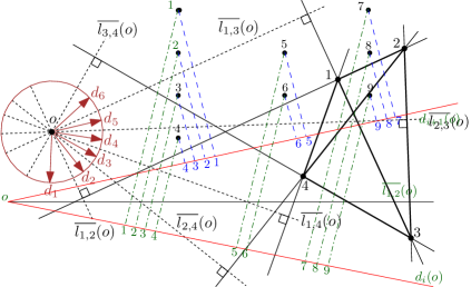
Assume, for now, that the point set does not contain three or more collinear points and, moreover, no two pairs of points are lying on parallel lines. Later on, we will describe how to deal with an arbitrary point set. Let be a point in the plane such that , and define set to consist of the lines with , passing through the origin (see the dashed lines in Fig. 16). Then, these lines partition the unit circle into sectors. Start from an arbitrary sector and let be the direction that bisects it. Consider then the next sector in ccw. order and let be the direction that bisects it. By continuing in this manner, we can define a circular sequence of pairwise non-opposite directions (see the red direction in Fig. 16). This construction of the direction set was outlined by Goodman and Pollack [26]. They showed that, for every , the linear orderings and differ exactly for the positions of two consecutive points and , namely immediately precedes in , while immediately follows in . By construction, for each direction , is in -general position. Also, can be computed in time by sorting the distinct slopes of the lines that are defined by point pairs in .
Obviously, each direction in defines a distinct monotone spanning path of ; to form the path, simply connect the points in order of appearance (of their projections) in . Moreover, for each monotone spanning path of there exists at least one direction of such that this path is -monotone. To see that, first consider the set of consecutive directions such that a path is -monotone. We call the monotonicity interval of . By Lemma 5, is an open sector of the unit circle. Now, simply observe that the boundaries of the monotonicity interval of path , , are lines in and, thus, at least one direction in is contained in the monotonicity interval. For , let be the monotone path defined by , and let be the length of . For implementation purposes, we assume that projections of points of in (and, consequently, path ) are stored in order of appearance in a doubly linked list of projection objects. Moreover, in order to be able to locate the projection of each point in the sorted list, we maintain with each point of a pointer to its projection object. Path and its length are easily computed in time by sorting the points in with respect to their projection on . Then, for each , path and its length are computed in time from and , by just updating the segments incident to the two points and of that exchange their position passing from to . Note that it is not hard to identify and , as they are the points that define the line that separates and in our construction; simply associate with each line in our construction the two points that define it. Hence, the algorithm computes all paths defined by and the lengths of these paths in time.

We now describe how to deal with the case where point set contains pairs of points lying on parallel lines. Note that these pairs of points may be lying on the same line, resulting to having more that three collinear points. For an example point set, refer to Fig. 17.
We again compute set consisting of the lines for every with , and sort the pairs of points with respect to the slopes of the corresponding lines in . In contrast with the “simple” point set examined in the previous paragraphs, we now end up with a smaller set of distinct slopes, where . In addition, these new distinct slopes partition the pairs of points into disjoints sets , each containing pairs of points having identical slopes for their corresponding lines in . From each set , we can select an arbitrary pair of points, say , , as the representative pair. We note that sets , can be computed in time by simply sorting the pairs of points with respect to the slopes of their corresponding lines in ; pairs of identical slope end up consecutive after sorting. We also observe that each set with induces a graph whose vertex set contains exactly the points involved in the pairs of . In addition, observe that each graph consists of connected components each of which is a clique and corresponds to points lying on the same line perpendicular to and, moreover, the projection of the points of each of these connected components on and do not overlap. In the example of Fig. 17, we have that and the three connected components (cliques) of are , and . Note that the connected components of all graphs with can be computed using depth first search in total time since there are exactly edges in all graphs together.
Thus, for the case of a point set containing pairs of points that lie on parallel lines, we can define the set of directions by considering only the distinct slopes of the lines in . It remains, however, to describe how we compute for two consecutive arbitrary directions and , , from . Let be the line separating and where is the representative pair of .
Observe that all collinear points lying on a line perpendicular to appear in reverse order in compared to the order they appear in ; see Fig. 17. Thus, in order to compute from , we have simply to identify these points. Of course, this has to be repeated for all different perpendicular lines to that contain at least a pair of points. However, we have already computed this information. The sets of collinear points perpendicular to correspond to the vertex sets with of the connected components of the graph . Thus, the extra cost for computing from is , which amounts to the reversion of the order of the points in the projections. We conclude that all such reversions can be computed in total time since the total number of edges in all computed graphs equals . ∎
Theorem 0.C.2
Given a set of points, a solution to the problem can be computed in time.
Proof
Let be the circular sequence of directions with as defined in the proof of Theorem 0.C.1. Recall that we can compute in time. By applying Theorem 0.B.1 to every pair of distinct directions , we consider a candidate -monotone tree for each set for which is in -general position. Since there are pairs, this takes time. To complete the proof we show that restricting to sets for which is in -general position is sufficient, namely we prove that if is a -monotone spanning tree for a set and is not in -general position, then there is a set such that is in -general position and is -monotone. This implies that if is a -monotone spanning tree and is not in -general position, then there is also a set such that is in -general position and is -monotone (with the previous reasoning for one or both the directions in ).
Let be a -monotone spanning tree, where . If is not in -general position, the orthogonal projection of on a line parallel to defines a sequence of points with . Some points of correspond to the projection of multiple points of ; each of these points is called a multiple point. By slightly rotating , we can obtain a direction such that: the projections of the points of that correspond to the same multiple point in form a consecutive subsequence of ; and replacing each such subsequence with a single point, we obtain . Finally, we show that is -monotone, where . Let be a path between two points and in ; if is -monotone then the points of are in -general position and thus the orthogonal projections of all points of correspond to distinct (non-multiple) points of . Hence the points in are also in -general position, and is also -monotone. ∎
Arguing as in the proof of Theorem 0.C.2, we get the following result for any .
Theorem 0.C.3
Given a set of point and any positive integer , there exists a function such that we can compute a minimum -directional monotone spanning tree of in time.
Proof
Let be the circular sequence of directions with as defined in the proof of Theorem 0.C.1, and which can be computed in time. By applying Theorem 5.1 to every set of distinct directions in , we consider all candidate -monotone trees over all sets of directions. Since there are sets, this takes time. By using an exchange argument as in the proof of Theorem 0.C.2, it can be proven that it is sufficient to restrict ourselves to sets of directions for which is -monotone. The statement follows. ∎
Appendix 0.D Additional Material for Section 6
Lemma 15
Let be a solution to the problem and let be a polygon vertex having . Then, for any two edges and that are consecutive in counter clockwise order around in and form an angle smaller than , it holds that . Equivalently, since the angle formed at by the edges from to any two consecutive polygon vertices is equal to , and are either consecutive polygon vertices, or one of them, say , coincides with and is the vertex following the anti-diametric of in ccw. order.
Proof
Consider the wedges in as defined by the lines ; see Fig. 18(a). Observe that the wedges partition the circle on which the polygon vertices lie into distinct circular arcs of equal length. To see this, consider an arbitrary wedge and let and be the points it intersects the unit circle centered at . Then, angle since is on the circle with center and, thus, the circular arcs formed by the wedges are also formed by equal angles at the center of the unit polygon. As a result, the wedges at also partition the polygon vertices into distinct sets, each consisting of two vertices, since vertices are all equally distanced on the circle; see Fig. 18(a).
Assume, for the sake of contradiction, that is greater than . That is, either and are non-consecutive vertices of the polygon or one of them, say , coincides with and is not the vertex ccw. to the anti-symmetric of with respect to . We consider these two cases separately.


- Case 1:
-
and are two non-consecutive polygon vertices (Fig. 18(b)). In this case, we define a circular sector (gray in Fig. 18(b)) by rotating the line counter-clockwise around untill it coincides with the line . The sector partitions into two subsets, namely, the set of points lying in and the set . All points in are connected to through some path either to or to , since edges and are two consecutive around edges (in ccw. order). Now, let and and be two paths in , such that is the last polygon vertex connected to in ccw. order and is the last polygon vertex connected to in clockwise order. Note that one of or may coincide with or , respectively. Observe that and are two consecutive vertices of the polygon. If and were not consecutive, then there would be a point between and which would not be connected to . Also, note that and should lie in different wedges of , since otherwise, due to Lemma 2, path would not be monotone. Let , for some direction , be the line passing between and . Then, path must be -monotone. To see that, observe that since path is -monotone with respect to at least one direction , its endpoints must lie on different sides of . But, given that only a single line through that is perpendicular to a direction in can pass between and , we conclude that path is -monotone. Thus, all vertices in lie between the parallel lines and .
This is a contradiction since the strip bounded by lines and contains only and, possibly, , but definitely neither nor . Note that the case where coincides with is similar, since then all vertices of path should lie between lines and . This is again, a contradiction, because the strip bounded by these two lines does not contain vertex .
- Case 2:
-
One of , coincides with , say , and is not the vertex following the anti-diagonal of in ccw. order. Line partitions the point set into two subsets, namely, set consisting of all points located on the same side of as point is, and set . Observe that all vertices in connect to through some path either to or or . We distinguish the following cases:
- Case 2a:
-
There is at least one vertex in that is connected to through (Fig. 18(c)). Again, let and and be two paths in such that is the last polygon vertex connected to in ccw. order and is the last polygon vertex connected to in clockwise order. As before, and are two consecutive polygon vertices lying in different wedges of and separated by , for some direction . Then, path must be -monotone, which only happens if points lie in the strip bounded by lines and . This is a contradiction since the only vertices in the strip are and, possibly, .
- Case 2b:
-
Vertex is a leaf in (Fig. 18(d)). Define as in Case 2a. Then, all points in are connected to only through and . Let and and be two paths such that is the last polygon vertex connected to in ccw. order and is the last polygon vertex connected to in clockwise order. Again, and are two consecutive polygon vertices lying in different wedges of and separated by , for some direction . Then, path is -monotone only if and both lie in the strip bounded by lines and ; a contradiction.
∎
See 12


Proof
Refer to Fig. 19(a). Consider an arbitrary wedge of . The wedge contains exactly two (consecutive) polygon vertices, say . Due to Property 2, is not connected in with both and ; otherwise, the path in would not be -monotone. Given that for every three consecutive polygon vertices exactly two of them lie in the same wedge, they can’t be all three incident to in . Then, by Lemma 15, can have at most two neighbors.
Consider now the case where is connected with (Fig. 19(b)). The wedge of which contains also contains two polygon vertices and that cannot be incident to in . One of them, say is anti-diametric to . Then, can only be connected to the polygon vertex lying in the neighboring wedge of the one containing and, thus, can have degree at most two. ∎
See 6.1
Proof
Let tree be a solution to the problem and assume that in not the -star with at its center. We first show that a vertex of degree one cannot be the endpoint of a chord. Let be an arbitrary polygon vertex that is a leaf of and let be the edge of that is incident to . If edge was a chord, then vertices on both sides of would connect in through and, thus, . However, this is not possible since, by Lemma 12, we have that . Therefore, is the endpoint of either a ray or an external edge. We further observe that, as is not the star, contains at least one external edge which has as an endpoint a polygon vertex of degree one. If this was not the case, then the polygon vertices of degree two together with would form one or more cycles, contradicting the acyclicity of .

Consider now a polygon vertex of degree one that is connected to with an external polygon edge. For easiness of presentation, we rotate the point set (and we renumber the vertices accordingly) so that coincides with vertex of Fig. 8(a). Note that since we have assumed that is even, it holds that and thus, one of the directions of , say , is horizontal.
We now examine how , which after the rotation and the renumbering is referred to as , is connected to in . Refer to Fig. 20. Vertex cannot be connected in to through the external edge . If it was, then, due to Lemma 15, must be in turn adjacent to . But then, both and fall in the same wedge of and, thus, the path cannot be monotone. Therefore, is connected with . Then, due to Lemma 15, is adjacent to which, in turn, is adjacent to , and so on. This path, continues until we reach the center . To see this, note that if the path ends before reaching then it ends at a polygon vertex of degree one. This contradicts the fact that is a connected spanning tree of . In addition, is reached through edge . If this was not the case and was adjacent in this path to a vertex which was before in ccw. order, the angle formed at by and its preceding edge in the path would be greater than , which is impossible due to Lemma 15. Thus, contains the path that starts at , ends at , and contains all points to the right of the vertical line through . We will show that cannot be of minimum length.
Consider tree formed by substituting the edges of path by rays from to the path vertices. Obviously is also monotone. To show that is not optimal, it suffices to show that the length of path is greater than the total length of the rays that substituted the edges of in . In other words it suffices to show that , where denotes the length of path . For the length of path , we have that (Lemma 16 and Lemma 17 in Appendix 0.D). Thus, tree is not of minimum length; a contradiction. We conclude that is the -star centered at . ∎
Lemma 16
.
Proof
For a sum of sine series we know from [34] that
| (1) |
Additionally, from trigonometry we know that
| (2) |
Be utilizing the above equations, we get:
∎
Lemma 17
, for .