Numerical null controllability of parabolic PDEs
using Lagrangian methods

Abstract

In this paper, we study several theoretical and numerical questions concerning the null controllability problems for linear parabolic equations and systems for several dimensions. The control is distributed and acts on a small subset of the domain. The main goal is to compute numerically a control that drives a numerical approximation of the state from prescribed initial data exactly to zero. We introduce a methodology for solving numerical controllability problems that is new in some sense. The main idea is to apply classical Lagrangian and Augmented Lagrangian techniques to suitable constrained extremal formulations that involve unbounded weights in time that make global Carleman inequalities possible. The theoretical results are validated by satisfactory numerical experiments for spatially $2$D and $3$D problems.

1 Introduction

Let $\Omega\subset\mathbb{R}^{d}$ ($d\geqslant 1$) be a bounded domain with boundary $\partial\Omega$ of class $C^{2}$ and let $T>0$ be given. Let us set $Q:=\Omega\times(0,T)$ and $\Sigma:=\partial\Omega\times(0,T)$. Also, for any open set $\omega\subset\Omega$, we will put $Q_{\omega}:=\omega\times(0,T)$.

Let $a\in W^{1,\infty}(Q)$ and $b\in L^{\infty}(Q)$ be given. We will suppose that $a$ satisfies $a(x,t)\geqslant a_{0}>0$ in $Q$ and, for convenience, we consider the differential operators $L$ and $L^{*}$, with

$$Ly=\partial_{t}y-\textrm{div}(a\nabla y)+by\quad\text{and}\quad L^{*}z=-\partial_{t}z-\text{div}(a\nabla z)+bz.$$

In this paper, we will mainly deal with distributed control problems for linear state systems of the form

$$\begin{cases}Ly=v\mathbbm{1}_{\omega}&\textrm{ in }Q,\\ y=0&\text{ on }\Sigma,\\ y(\cdot\,,0)=y_{0}&\textrm{ in }\Omega,\end{cases}$$ (1.1)

where $\omega\subset\Omega$ is a (maybe small) non-empty open set, $\mathbbm{1}_{\omega}$ is the associated characteristic function, $v\in L^{2}(Q_{\omega})$ and $y_{0}\in L^{2}(\Omega)$. Here, $v=v(x,t)$ is the control and $y=y(x,t)$ is the state.

It is well known that, for every $v\in L^{2}(Q_{\omega})$, there exists a unique weak solution $y$ to (1.1), with

$$y\in C^{0}([0,T];L^{2}(\Omega))\cap L^{2}(0,T;H_{0}^{1}(\Omega)).$$

The null controllability problem for (1.1) can be formulated as follows: for each $y_{0}\in L^{2}(\Omega)$, find a control $v\in L^{2}(Q_{\omega})$ such that the corresponding solution to (1.1) satisfies

$$y(x,T)=0,\quad x\in\Omega.$$ (1.2)

In the sequel, we will respectively denote by $(\cdot\,,\cdot)$ and $\|\cdot\|$ the usual scalar product and norm in $L^{2}(\Omega)$ and the symbol $C$ will stand for a generic positive constant.

1.1 Literature

Controllability issues for PDEs have attracted the attention of the scientific community since the 80’s; we mention [14, 15, 22, 4] for a general overview. In particular, for the null controllability problem for the heat equation, we mention [10] and [16], where different approaches have been shown; see also [6].

The regularity properties of the trajectories play an important role in the field. Thus, in the case of a parabolic equation, the regularization effect leads to some nontrivial difficulties that were exhibited numerically for the first time in [3], where the authors try to find controls of minimal $L^{2}$ norm.

Let us introduce two functions $\rho$ and $\rho_{0}$ with

$$\begin{cases}\rho=\rho(x,t),\,\rho_{0}=\rho_{0}(x,t)\textrm{ are continuous and }\geqslant\rho_{*}>0\textrm{ in }Q,\\ \displaystyle\min_{x\in\overline{\Omega}}\rho(x,t)\to+\infty\text{ and }\min_{x\in\overline{\Omega}}\rho_{0}(x,t)\to+\infty\text{ as }t\to T^{-}\end{cases}$$ (1.3)

and let us set

$$\mathcal{U}:=\rho_{0}^{-1}L^{2}(Q_{\omega})=\{v\in L^{2}(Q_{\omega}):\rho_{0}v\in L^{2}(Q_{\omega})\},$$

$$\mathcal{Y}:=\rho^{-1}L^{2}(Q)=\{y\in L^{2}(Q_{\omega}):\rho y\in L^{2}(Q)\}$$

and

$$\mathcal{C}(y_{0},T):=\{(y,v)\in\mathcal{Y}\times\mathcal{U}:y\textrm{ solves }\eqref{eq:main:01}\}.$$

We will consider the constrained extremal problem

$$\begin{cases}\textrm{Minimize }\displaystyle J(y,v)=\dfrac{1}{2}\iint_{Q}\rho^{2}|y|^{2}\,dx\,dt+\dfrac{1}{2}\iint_{Q_{\omega}}\rho_{0}^{2}|v|^{2}\,dx\,dt,\\ \textrm{Subject to }(y,v)\in\mathcal{C}(y_{0},T),\end{cases}$$ (1.4)

introduced in the 90’s by Fursikov and Imanuvilov; see [10] and the references therein.

Remark 1.1.

It is worth mentioning that, in (1.4), the null controllability requirement is implicitly imposed in the requirement $(y,v)\in\mathcal{C}(y_{0},T)$. In fact, it is known that $\mathcal{C}(y_{0},T)\neq\emptyset$ and any couple $(y,v)\in\mathcal{C}(y_{0},T)$ provides a solution to the null controllability problem (1.1)–(1.2). $\Box$

In this paper, we focus on the analysis and resolution of (1.4) by using Lagrangian and Augmented Lagrangian methods.

From the numerical controllability viewpoint, it is natural to consider the computation of minimal $L^{2}$-norm null controls. This corresponds to (1.4) with $\rho\equiv 0$ and $\rho_{0}\equiv 1$ and has been considered by Carthel et. al. in [3] and then by other authors.

The solution can be achieved as follows. For every $\varphi_{0}\in L^{2}(\Omega)$, we consider the associated backward system

$$\begin{cases}L^{*}\varphi=0&\textrm{ in }Q,\\ \varphi=0&\text{ on }\Sigma,\\ \varphi(\cdot\,,T)=\varphi_{0}&\text{ in }\Omega.\end{cases}$$ (1.5)

Then, the null control of minimal norm in $L^{2}(Q_{\omega})$ is given by $v=\hat{\varphi}\mathbbm{1}_{\omega}$, where $\hat{\varphi}$ is the solution to (1.5) that corresponds to $\hat{\varphi}_{0}$ and $\hat{\varphi}_{0}$, minimizes the functional

$$I(\varphi_{0}):=\dfrac{1}{2}\iint_{Q_{\omega}}|\varphi(x,t)|^{2}\,dx\,dt+\int_{\Omega}y_{0}(x)\varphi(x,0)\,dx,$$

over the Hilbert space $\mathcal{H}$, given by the completion of $L^{2}(\Omega)$ with respect to the norm

$$\|\varphi_{0}\|_{\mathcal{H}}:=\|\varphi\|_{L^{2}(Q_{\omega})}.$$

Note that the mapping $\varphi_{0}\mapsto\|\varphi_{0}\|_{\mathcal{H}}$ is a semi-norm in $\mathcal{D}(\Omega)$. In view of the unique continuation property satisfied by the solutions to the systems (1.5), it is in fact a pre-Hilbertian norm. Hence, the completion of $\mathcal{D}(\Omega)$ for this norm can be considered.

Furthermore, one has the observability inequality

$$\|\varphi(\cdot\,,0)\|^{2}\leqslant C\iint_{Q_{\omega}}|\varphi|^{2}\,dx\,dt\quad\forall\varphi_{0}\in L^{2}(\Omega)$$ (1.6)

and, consequently, the coerciveness of the functional $I$ in $\mathcal{H}$ is ensured. Note that (1.6) is a consequence of some appropriate global Carleman estimates, see for instance [10] and [6].

As explained in [21], one has $H^{-s}(\Omega)\hookrightarrow\mathcal{H}$ for all $s>0$ with continuous embedding. For a proof of this assertion in 1-D case, see [20]. Accordingly, the minimization of $I$ is numerically ill-posed: it does not seem easy to find a family of finite-dimensional ordered spaces that approximate the functions $\varphi_{0}$ in the sense of the $\mathcal{H}$ norm as the dimension grows to infinity. For this reason, in [3] the authors considered regularized approximate controllability problems, replacing $I$ by $I_{\epsilon}$, where

$$I_{\epsilon}(\varphi_{T}):=I(\varphi_{T})+\epsilon\|\varphi_{T}\|_{L^{2}},\quad\epsilon>0.$$

The minimizers $\varphi_{T,\epsilon}\in L^{2}(\Omega)$ and therefore the corresponding controls $v_{\epsilon}$ produce states $y_{\epsilon}$ that satisfy $\|y_{\epsilon}(\cdot\,,T)\|_{L^{2}}\leqslant\epsilon$. The main advantage of this approach is that it can handle various boundary conditions and can be adapted to different types of parabolic and hyperbolic equations. However, for small $\epsilon$, the controls obtained by this method oscillate near the final time, unless a careful approximation and/or penalization process is performed; see [1, 2, 3, 11, 12, 21] for more details.

An alternative is the so called flatness approach. This is a direct method for which the solution relies on the computation of the sums of appropriate series expansions. The corresponding partial sums are easy to compute and provide accurate numerical approximations of both the control and the state. The main advantage of this method is that it provides explicit control laws for certain problems. However, its implementation for high-dimensional systems can be cumbersome and the requirement to the system to be flat (i.e. to have time independent coefficients) makes the scope of the method limited; see [17, 18, 19] for more details.

A second alternative is given by the space-time strategy introduced in [7]. It relies on the Fursikov-Imanuvilov formulation of controllability problems, where a weighted integral involving both variables, state and control, is introduced, see [10] and the references therein; see also [6].

In this method, the task is reduced to solve a second-order in time and fourth-order in space PDE system. The main advantage is that the strong convergence of the approximations is obtained from Céa’s Lemma and a good choice of the associated finite dimensional approximation spaces. However, the numerical solution via a direct method requires in practice $C^{0}$ in time and $C^{1}$ in space finite elements and consequently is not easy to handle in high dimension.

The $C^{1}$ regularity drawback can be circumvented by introducing mixed formulations but this is not to our knowledge completely well-justified from the theoretical viewpoint. Moreover, for high dimension problems, the method is far from simple; for instance, to solve a control problem for $3$D heat equation, at least $\mathbb{P}_{1}$-Lagrange $4$D finite elements are needed.

1.2 Plan of the paper

In this paper, we will apply other methods that also start from the space-time strategy. The idea is to introduce some Lagrangian (saddle-point) reformulations of (1.4). The techniques are relatively well known in many other contexts and have been applied since several decades to various PDE problems, see [9].

Let us mention some advantages of the use of Lagrangian and Augmented Lagrangian formulations in the context of controllability problems:

• They are easy to adapt to parabolic problems with nonzeo right-hand sides with a suitable exponential decay as $t\to T^{-}$.

• Various kinds of boundary conditions can be considered.

• The well-posedness of the numerical approximations can be rigorously justified.

• The methods are useful for high dimension problems, where there are very few efficient techniques. Thus, the implementation for $3$D parabolic equations is similar to the $2$D case, and does not bring extra difficulties.

• The methods are compatible (and improvable) with adaptive mesh refinement.

The paper is organized as follows.

Section 2 is devoted to analyze the extemal problem (1.4), a family of “truncated” approximations and their properties. In Section 3, we introduce Lagrangian and Augmented Lagrangian (saddle-point) reformulations of he truncated problems. Then, several related algorithms of the Uzawa kind are presented and described in Section 4. Section 5 is devoted to the null controllability problem for the Stokes system and its Lagrangian reformulations. In Section 6, we present with detail the results of several numerical experiments for $2$D and $3$D problems concerning the heat equation and the Stokes system. Finally, Section 7 contains some conclusions, additional comments and open questions.

2 Truncation of the extremal control problem

In order to formulate with detail our first main problem, we consider a function $\eta^{0}\in C^{2}(\overline{\Omega})$ such that

$$\eta^{0}=0\text{ on }\partial\Omega,\quad|\nabla\eta^{0}|>0\text{ in }\Omega\setminus\overline{\omega}\quad\text{and}\quad\partial_{\nu}\eta^{0}<0\text{ on }\partial\Omega.$$ (2.1)

The existence of $\eta^{0}$ is proved in [10] for $\Omega$ of class $C^{2}$ and arbitrary $\omega$. As we will see in Section 6, it is also possible to construct explicit functions $\eta^{0}$ when $\Omega$ is a bounded domain with polygonal or polyhedrical boundary.

Let us set

$$\alpha(x,t):=K_{1}\dfrac{e^{K_{2}}-e^{\eta^{0}(x)}}{T-t},\quad\rho(x,t):=e^{\alpha(x,t)}\quad\text{and}\quad\rho_{0}(x,t):=(T-t)^{3/2}\rho(x,t),$$ (2.2)

where $K_{1},K_{2}>0$ are sufficiently large. It is immediate to check that these functions $\rho$ and $\rho_{0}$ satisfy (1.3).

Let us introduce the linear operator $M:L^{2}(Q_{\omega})\to L^{2}(Q)$ with $Mv:=y$, where $y$ is the weak solution to the linear problem

$$\begin{cases}Ly=v\mathbbm{1}_{\omega}&\text{ in }Q,\\ y=0&\text{ on }\Sigma,\\ y(\cdot\,,0)=0&\text{ in }\Omega.\end{cases}$$

Its adjoint $M^{*}:L^{2}(Q)\to L^{2}(Q_{\omega})$ is given by $M^{*}q=z|_{Q_{\omega}}$, where $z$ is the weak solution to

$$\begin{cases}L^{*}z=q&\text{ in }Q,\\ z=0&\text{ on }\Sigma,\\ z(\cdot\,,T)=0&\text{ in }\Omega.\end{cases}$$

In the sequel, we denote by $\overline{y}$ the solution to (1.1) with $v\equiv 0$. Then the set $\mathcal{C}(y_{0},T)$ in (1.4) can be written in the form

$$\mathcal{C}(y_{0},T)=\{(y,v)\in\mathcal{Y}\times\mathcal{U}:y=Mv+\overline{y}\}.$$

Let us introduce the linear space

$$P_{0}:=\{q\in C^{2}(\overline{Q}):q=0\text{ on }\Sigma\}.$$

In this space, the bilinear form

$$(p,q)_{P}:=\iint_{Q}\rho^{-2}L^{*}p\,L^{*}q\,dx\,dt+\iint_{Q_{\omega}}\rho_{0}^{-2}p\,q\,dx\,dt$$

is in fact a scalar product. Indeed, if we have $q\in P_{0}$, $L^{*}q=0$ in $Q$ and $q=0$ in $Q_{\omega}$, from the unique continuation property for parabolic equations, we deduce that $q\equiv 0$.

Let $P$ be the completion of $P_{0}$ for this scalar product (a Hilbert space). We have the following result:

Proposition 2.1.

Let $\rho,\rho_{0}$ be the functions defined in (2.2). Then (1.4) has a unique minimizer $(y,v)\in\mathcal{Y}\times\mathcal{U}$. Moreover, we have the following characterization:

$$y=-\rho^{-2}q,\quad v=\rho_{0}^{-2}M^{*}q.y=-\rho^{-2}L^{*}p,\quad v=\rho_{0}^{-2}p\big{|}_{Q_{\omega}},$$

where $p\in P$ is the unique solution to the variational (Lax-Milgram-like) problem

$$\begin{cases}\displaystyle\iint_{Q}\rho^{-2}L^{*}p\,L^{*}q\,dx\,dt+\iint_{Q_{\omega}}\rho_{0}^{-2}p\,q\,dx\,dt=\int_{\Omega}y_{0}(x)\,q(x,0)\,dx,\\ \forall q\in P,\quad p\in P.\end{cases}$$ (2.3)

The proof is given in [10]; see also [7, Proposition $2.1$].

Remark 2.2.

In this result, the hypothesis that the Carleman weights $\rho$ and $\rho_{0}$ are as in (2.2) is crucial. Indeed, this is essential to prove the continuity of the linear form in the Lax-Milgram problem (2.3), thanks to a Carleman inequality. $\Box$

Remark 2.3.

Note that the solution to (2.3) solves, at least in the weak sense, the following fourth-order in space and second-order in time problem:

$$\begin{cases}L(\rho^{-2}L^{*}p)+\rho_{0}^{-2}p\,\mathbbm{1}_{\omega}=0&\text{ in }Q,\\ p=0,\quad\rho^{-2}L^{*}p=0&\text{ on }\Sigma,\\ \rho^{-2}L^{*}p(\cdot\,,0)=y_{0},\quad\rho^{-2}L^{*}p(\cdot\,,T)=0&\text{ in }\Omega;\end{cases}$$

see [10]. $\Box$

Remark 2.4.

Note also that the solution to (2.3) solves the following extremal problem:

$$\begin{cases}\textrm{Minimize }\displaystyle J^{*}(q):=\dfrac{1}{2}\iint_{Q}\rho^{-2}|L^{*}q|^{2}\,dx\,dt+\dfrac{1}{2}\iint_{Q_{\omega}}\rho_{0}^{-2}|q|^{2}\,dx\,dt-\int_{\Omega}y_{0}(x)q(x,0)\,dx,\\ \textrm{Subject to }q\in P.\end{cases}$$ (2.4)

In some sense, (2.4) can be viewed as a dual problem of (1.4). $\Box$

2.1 A truncated problem

A detailed characterization of the minimizer of (1.4) is furnished by Proposition 2.1. A related numerical treatment was performed in [7] by using direct and mixed variational approximations of (2.3).

In order to apply Lagrangian and Augmented Lagrangian methods avoiding technical difficulties, let us introduce the problem

$$\begin{cases}\textrm{Minimize }\displaystyle J_{R}(y,v):=\dfrac{1}{2}\iint_{Q}\rho_{R}^{2}|y|^{2}\,dx\,dt+\dfrac{1}{2}\iint_{Q_{\omega}}\rho_{0}^{2}|v|^{2}\,dx\,dt,\\ \textrm{Subject to }(y,v)\in\widetilde{\mathcal{C}}(y_{0},T),\end{cases}$$ (2.5)

where $R>0$,

$$\rho_{R}(x,t):=\min(R,\rho(x,t)),\quad(x,t)\in Q$$ (2.6)

and

$$\widetilde{\mathcal{C}}(y_{0},T):=\{(y,v)\in L^{2}(Q)\times\mathcal{U}:y\textrm{ solves }\eqref{eq:main:01}\}.$$

We point out that the new weight $\rho_{R}$ does not blow up as $t\to T^{-}$.

Recall that, for each $y_{0}\in L^{2}(\Omega)$, the weak solution to (1.1) can be written in the form $y=Mv+\overline{y},$ where $M$ was introduced at the beginning of Section 3. Accordingly, we can rewrite (2.5) in such a way that the results of [5] concerning Lagrange methods can be applied.

Thus, let us introduce the convex functions

$$F_{R}:L^{2}(Q)\to\mathbb{R},\ \ G:\mathcal{U}\to\mathbb{R}\ \text{ and }\ \overline{F}_{R}:L^{2}(Q)\to\mathbb{R},$$

with

$$F_{R}(y):=\dfrac{1}{2}\iint_{Q}\rho_{R}^{2}|y|^{2}\,dx\,dt,\quad G(v):=\dfrac{1}{2}\iint_{Q_{\omega}}\rho_{0}^{2}|v|^{2}dx\,dt\quad\text{and}\quad\overline{F}_{R}(z):=F_{R}(z+\overline{y}).$$

Observe that, for every $(y,v)\in\widetilde{\mathcal{C}}(y_{0},T)$, one has

$$J_{R}(y,v)=I_{R}(v):=\overline{F}_{R}(Mv)+G(v)\quad\forall\,v\in\mathcal{U}.$$

Here, $I_{R}:\mathcal{U}\to\mathbb{R}$ is a well-defined proper, continuous and strictly convex function and (2.5) is equivalent to the unconstrained extremal problem

$$\begin{cases}\textrm{Minimize }I_{R}(v),\\ \textrm{Subject to }v\in\mathcal{U}.\end{cases}$$ (2.7)

Obviously, for every $R>0$, (2.7) is uniquely solvable. Furthermore, the following result holds:

Proposition 2.5.

Let $v_{R}$ be, for each $R>0$, the unique solution to (2.7). Then one has

$$v_{R}\to\widehat{v}\text{ strongly in }\mathcal{U}\text{ as }R\to+\infty,$$ (2.8)

where $\widehat{v}$ is, together with $\widehat{y}=M\widehat{v}+\overline{y}$, the unique solution to (1.4).

Proof.

First, we note that, for any $R>0$,

$$I_{R}(\widehat{v})=\dfrac{1}{2}\iint_{Q}\rho_{R}^{2}|M\widehat{v}+\overline{y}|^{2}\,dx\,dt+\dfrac{1}{2}\iint_{Q_{\omega}}\rho_{0}^{2}|\widehat{v}|^{2}\,dx\,dt\leqslant J(\widehat{y},\widehat{v}).$$

Consequently, each $v_{R}$ satisfies

$$I_{R}(v_{R})\leqslant I_{R}(\widehat{v})\leqslant J(\widehat{y},\widehat{v})\quad\forall R>0.$$ (2.9)

This shows that $\rho_{R}(Mv_{R}+\overline{y})$ is uniformly bounded in $L^{2}(Q)$ and $\rho_{0}v_{R}$ is uniformly bounded in $L^{2}(Q_{\omega})$. Therefore, at least for a subnet, one has that there exist $z\in L^{2}(Q)$ and $w\in L^{2}(Q_{\omega})$ with

$$\rho_{R}(Mv_{R}+\overline{y})\to z\text{ weakly in }L^{2}(Q)\ \text{ and }\ \rho_{0}v_{R}\to w\text{ weakly in }L^{2}(Q_{\omega})\text{ as $R\to+\infty$.}$$ (2.10)

Let us set $\tilde{y}:=\rho^{-1}z$ and $\tilde{v}:=\rho_{0}^{-1}w$. It is then clear, from (2.10) and Lebesgue’s Theorem, that

$$v_{R}\to\tilde{v}\text{ weakly in }L^{2}(Q_{\omega})\ \text{ and }\ Mv_{R}+\overline{y}\to\tilde{y}\text{ weakly in }L^{2}(Q).$$

In fact, $\tilde{y}$ is the state associated to $\tilde{v}$ with initial condition $y_{0}$ and $Mv_{R}+\overline{y}$ converges strongly to $\tilde{y}$ in $L^{2}(Q)$, thanks to the usual parabolic compactness results. Furthermore, one has

$$J(\tilde{y},\tilde{v})\leqslant \liminf_{R\to\infty}\left(\dfrac{1}{2}\iint_{Q}\rho_{R}^{2}|Mv_{R}+\overline{y}|^{2}\,dx\,dt+\dfrac{1}{2}\iint_{Q_{\omega}}\rho_{0}^{2}|v_{R}|^{2}\,dx\,dt\right)$$

$$\leqslant \lim_{R\to\infty}\left(\dfrac{1}{2}\iint_{Q}\rho_{R}^{2}|Mv+\overline{y}|^{2}\,dx\,dt+\dfrac{1}{2}\iint_{Q_{\omega}}\rho_{0}^{2}|v|^{2}\,dx\,dt\right)=J(y,v),$$

for every $(y,v)\in\mathcal{Y}\times\mathcal{U}$. Hence, $(\tilde{y},\tilde{v})=(\widehat{y},\widehat{v})$.

Finally, we also deduce from the properties satisfied by the $v_{R}$ that

$$\limsup_{R\to\infty}\left(\iint_{Q}\rho_{R}^{2}|Mv_{R}+\overline{y}|^{2}\,dx\,dt+\iint_{Q_{\omega}}\rho_{0}^{2}|v_{R}|^{2}\,dx\,dt\right)\leqslant J(y,v)\quad\forall(y,v)\in\mathcal{Y}\times\mathcal{U},$$

whence this upper limit is bounded from above by $J(\widehat{y},\widehat{v})$ and then

$$\lim_{R\to\infty}\left(\iint_{Q}\rho_{R}^{2}|Mv_{R}+\overline{y}|^{2}\,dx\,dt+\iint_{Q_{\omega}}\rho_{0}^{2}|v_{R}|^{2}\,dx\,dt\right)=J(\widehat{y},\widehat{v}).$$

Therefore, $v_{R}\to\widehat{v}$ strongly in $\mathcal{U}$, $\rho_{R}(Mv_{R}+\overline{y})\to\rho\widehat{y}$ strongly in $L^{2}(Q)$ and (2.8) holds. ∎

As a consequence of this result, we see that an appropriate strategy to solve the null controllability problem for (1.1) can be to compute the solution to (2.7) for large $R$ and then take $y_{R}=Mv_{R}+\overline{y}$ as an approximation to $\widehat{y}$.

2.2 Estimates of the convergence rate of the truncated solutions

The following result holds:

Proposition 2.6.

Let $v_{R}$ be the solution to the extremal problem (2.7) and let us set $y_{R}=Mv_{R}+\overline{y}$. There exists a positive constant $C$ independent of $R$ such that

$$\|y_{R}(\cdot\,,T)\|_{H_{0}^{1}(\Omega)}\leqslant C\,\dfrac{|\log R|}{R}\quad\forall R>0.$$ (2.11)

Proof.

The proof relies on a suitable energy estimate of $\rho_{R}^{-1}q$ at times close to $T$, with a right-hand side that does not depend of $R$.

It can be assumed that $R$ is large enough. Then, let us introduce $\rho_{0}^{*}$ with

$$\rho_{0}^{*}(t)=\min_{x\in\overline{\Omega}}\rho_{0}(x,t).$$

Denote by $T_{R}$ the time at which $\rho_{0}^{*}(T_{R})=R$. Then, since $\rho_{0}^{*}$ is increasing, we have

$$\rho_{0}(x,t)\geqslant R\quad\forall x\in\Omega,\ \ \forall t\in[T_{R},T].$$ (2.12)

Now, let $T_{1,R},T_{2,R}\in(T_{R},T)$ be given with $T-T_{1,R}\leqslant 1$ and $T_{2,R}-T_{1,R}\geqslant(T-T_{R})/2$. Then, let us consider a cut-off function $\psi_{R}\in C^{\infty}([0,T])$ satisfying

$$0\leqslant\psi_{R}\leqslant 1\text{ in }[0,T],\quad\psi_{R}=0\text{ in }[0,T_{1,R}]\quad\text{and}\quad\psi_{R}=1\text{ in }[T_{2,R},T]$$

and let us set $z:=\psi_{R}\,\rho_{R}\,y_{R}$. Then $z$ solves the problem

$$\begin{cases}Lz=(\chi_{R}\rho_{R})v_{R}\mathbbm{1}_{\omega}+\partial_{t}(\chi_{R}\rho_{R})y_{R}&\text{ in }Q,\\ z=0&\text{ on }\Sigma,\\ z(\cdot\,,0)=0&\text{ in }\Omega.\end{cases}$$

Taking into account (2.12) and (2.9), we find that

$$\begin{array}[]{l}\displaystyle\iint_{Q}|Lz|^{2}\,dx\,dt\leqslant\iint_{\omega\times(T_{1,R},T)}\rho_{0}^{2}|v_{R}|^{2}\,dx\,dt+\iint_{\omega\times(T_{1,R}},{T_{2,R})}(\chi^{\prime}_{R})^{2}\rho_{R}^{2}|y_{R}|^{2}\,dx\,dt\\ \vskip 3.0pt plus 1.0pt minus 1.0pt\cr\displaystyle\phantom{\iint_{Q}|Lz|^{2}\,dx\,dt}\leqslant\iint_{\omega\times(0,T)}\rho_{0}^{2}|v_{R}|^{2}\,dx\,dt+\frac{C}{(T_{2,R}-T_{1,R})^{2}}\iint_{Q}\rho_{R}^{2}|y_{R}|^{2}\,dx\,dt\\ \vskip 3.0pt plus 1.0pt minus 1.0pt\cr\displaystyle\phantom{\iint_{Q}|Lz|^{2}\,dx\,dt}\leqslant\frac{C}{(T_{2,R}-T_{1,R})^{2}}J(\widehat{y},\widehat{v}),\end{array}$$

where $\widehat{v}$ is the solution to (1.4) and $\widehat{y}=M\widehat{v}+\overline{y}$. Furthermore, from the particular form of $\rho_{0}$, we now that $T-T_{R}\leqslant C/|\log R|$ and this implies

$$\|z\|_{C^{0}(0,T];H_{0}^{1}(\Omega))}^{2}+\|z\|_{L^{2}(0,T;H_{0}^{1}(\Omega)\cap H^{2}(\Omega))}^{2}\leqslant\frac{C}{(T_{2,R}-T_{1,R})^{2}}J(\widehat{y},\widehat{v})\leqslant CJ(\widehat{y},\widehat{v})|\log R|^{2},$$

for some $C>0$ independent of $R$. Hence,

$$\|\rho_{R}^{-1}(\cdot\,,T)q_{R}(\cdot\,,T)\|_{H_{0}^{1}}\leqslant\|\rho_{R}^{-1}q_{R}\|_{C^{0}([T_{2,R},T];H_{0}^{1}(\Omega))}\leqslant CJ(\widehat{y},\widehat{v})^{1/2}|\log R|$$

and, from the Cauchy-Scharwz inequality and the fact that $\rho_{R}(\cdot\,,T)\equiv R$ in $\Omega$, we find that

$$\|\nabla y_{R}(\cdot\,,T)\|=\|\rho_{R}(\cdot\,,T)^{-1}\nabla(\rho_{R}(\cdot\,,T)q_{R}(\cdot\,,T))\|\leqslant\dfrac{C\,|\log R|}{R}.$$

This implies (2.11) and ends the proof. ∎

3 Solving the truncated extremal problem using Lagrange methods

In this section, we use more or less standard results from convex analysis to reformulate (2.7) appropriately and deduce related efficient algorithms.

3.1 The Lagrangian

Let us introduce the convex functions

$$F_{R}:L^{2}(Q)\to\mathbb{R},\ \ G:\mathcal{U}\to\mathbb{R}\ \text{ and }\ \overline{F}_{R}:L^{2}(Q)\to\mathbb{R},$$

with

$$F_{R}(y):=\dfrac{1}{2}\iint_{Q}\rho_{R}^{2}|y|^{2}\,dx\,dt,\quad G(v):=\dfrac{1}{2}\iint_{Q_{\omega}}\rho_{0}^{2}|v|^{2}dx\,dt\quad\text{and}\quad\overline{F}_{R}(z):=F_{R}(z+\overline{y}).$$

For every $R>0$, we will consider the family of perturbations $\{\Phi_{R}(\cdot\,,p)\}_{p\in L^{2}(Q)}$, defined as follows:

$$\Phi_{R}(v,p):=\overline{F}_{R}(Mv-p)+G(v)\quad\forall v\in\mathcal{U},\ \ \forall p\in L^{2}(Q).$$

We will adapt the strategy and results in [5].

Clearly, $\Phi(v,0)=I_{R}(v)$ for all $v\in\mathcal{U}$. Moreover, the convex conjugate $\Phi_{R}^{*}$ of $\Phi_{R}$ is given by

$$\Phi_{R}^{*}(w,q)=\overline{F}_{R}^{*}(-q)+G^{*}(M^{*}(w+q)),$$

where

$$\overline{F}_{R}^{*}(u):=\dfrac{1}{2}\iint_{Q}\rho_{R}^{-2}|u|^{2}\,dx\,dt-\iint_{Q}\overline{y}u\,dx\,dt,\quad G^{*}(w):=\dfrac{1}{2}\iint_{Q_{\omega}}\rho_{0}^{-2}|w|^{2}dx\,dt.$$

In particular, we see that

$$\Phi_{R}^{*}(0,q)= \overline{F}_{R}^{*}(-q)+G^{*}(M^{*}q)$$

$$= \dfrac{1}{2}\iint_{Q}\rho_{R}^{-2}|q|^{2}\,dx\,dt+\dfrac{1}{2}\iint_{Q_{\omega}}\rho_{0}^{-2}|M^{*}q|^{2}\,dx\,dt+\iint_{Q}q\overline{y}\,dx\,dt$$

for every $q\in L^{2}(Q)$.

The dual problem of (2.7) is

$$\begin{cases}\textrm{Maximize }-\Phi_{R}^{*}(0,q),\\ \textrm{Subject to }q\in L^{2}(Q),\end{cases}$$ (3.1)

while the Lagrangian associated with $\Phi_{R}$ reads

$$L_{R}(v,q):= \leavevmode\nobreak\ -F_{R}^{*}(-q)+G(v)-(q,Mv+\overline{y})_{L^{2}(Q)}$$

$$= \leavevmode\nobreak\ \dfrac{1}{2}\iint_{Q_{\omega}}\rho_{0}^{2}|v|^{2}\,dx\,dt-\dfrac{1}{2}\iint_{Q}\rho_{R}^{-2}|q|^{2}\,dx\,dt-\iint_{Q}q(Mv+\overline{y})\,dx\,dt.$$

Theorem 3.1.

Let $R>0$ be given and let the functions $\rho_{R}$ and $\rho_{0}$ be as in (2.1), (2.2) and (2.6). Then, one has:

• The extremal problems (2.7) and (3.1) are uniquely solvable.

• The following identities hold:

  $$\inf_{v\in\mathcal{U}}I_{R}(v)=\inf_{v\in\mathcal{U}}\sup_{q\in L^{2}(Q)}L_{R}(v,q)\ \text{ and }\ \sup_{q\in L^{2}(Q)}-\Phi_{R}^{*}(0,q)=\sup_{q\in L^{2}(Q)}\inf_{v\in\mathcal{U}}L_{R}(v,q).$$

• Let $v_{R}\in\mathcal{U}$ and $q_{R}\in L^{2}(Q)$ be the solutions respectively to (2.7) and (3.1). Then $(v_{R},q_{R})$ is the unique saddle-point of $L_{R}$, that is, the unique couple in $\mathcal{U}\times L^{2}(Q)$ satisfying

  $$\inf_{v\in\mathcal{U}}\sup_{q\in L^{2}(Q)}L_{R}(v,q)=L_{R}(v_{R},q_{R})=\sup_{q\in L^{2}(Q)}\inf_{v\in\mathcal{U}}L_{R}(v,q).$$

• The following optimality characterization holds

  $$\begin{cases}\overline{F}_{R}(Mv_{R})+\overline{F}_{R}^{*}(-q_{R})=-(Mv_{R},q_{R})_{L^{2}(Q)},\\ G(v_{R})+G^{*}(M^{*}q_{R})=\langle M^{*}q_{R},v_{R}\rangle_{\mathcal{U}^{\prime},\mathcal{U}}.\end{cases}$$ (3.2)

  Consequently, setting $y_{R}:=Mv_{R}+\overline{y}$, one has

  $$y_{R}=-\rho_{R}^{-2}q_{R},\quad v_{R}=\rho_{0}^{-2}M^{*}q_{R}.$$ (3.3)

All these assertions are immediate consequences of the results in [5] (see Chapter III, Proposition 4.2) except the fact that (3.2) implies (3.3). But this follows from the values taken by $\overline{F}_{R}$ and $G$ and their convex conjugate functions.

Indeed, for instance, the first identity in (3.2) reads

$$\dfrac{1}{2}\iint_{Q}\rho_{R}^{2}|Mv_{R}+\overline{y}|^{2}\,dx\,dt+\dfrac{1}{2}\iint_{Q}\rho_{R}^{-2}|q_{R}|^{2}\,dx\,dt=-\iint_{Q}(Mv_{R}+\overline{y})q_{R}\,dx\,dt,$$

that is to say,

$$\iint_{Q}|\rho_{R}y_{R}+\rho_{R}^{-1}q_{R}|^{2}\,dx\,dt=0$$

and the first equality in (3.3) is found. A similar argument from the second identity in (3.2) leads to the second one.

3.2 The Augmented Lagrangian

Before going further, let us introduce the function

$$\mathcal{L}_{R}(y,v,q):=J_{R}(v,y)-(q,Mv+\overline{y}-y)_{L^{2}(Q)}\quad\forall(y,v,q)\in L^{2}(Q)\times\mathcal{U}\times L^{2}(Q).$$

The unique saddle-point $(v_{R},q_{R})$ of $L_{R}$ is related to the unique saddle-point $(v_{R},y_{R},q_{R})$ of $\mathcal{L}_{R}$ through the identity $y_{R}=Mv_{R}+\overline{y}$.

Indeed, we have by definition

$$L_{R}(v,q)=\inf_{p\in L^{2}(Q)}\{\Phi_{R}(v,p)-(q,p)_{L^{2}(Q)}\}=\inf_{y\in L^{2}(Q)}\mathcal{L}_{R}(y,v,q),$$

where we have used the change of variables $y=Mv+\overline{y}-p$. Then, it is clear that

$$\sup_{q\in L^{2}(Q)}\inf_{v\in\mathcal{U}}L_{R}(v,q)=\sup_{q\in L^{2}(Q)}\inf_{(y,v)\in L^{2}(Q)\times\mathcal{U}}\mathcal{L}_{R}(y,v,q)$$

and also

$$\inf_{v\in\mathcal{U}}\sup_{q\in L^{2}(Q)}L_{R}(v,q)=\inf_{(y,v)\in L^{2}(Q)\times\mathcal{U}}\sup_{q\in L^{2}(Q)}\mathcal{L}_{R}(y,v,q).$$

Consequently, for every $R>0$, $\mathcal{L}_{R}$ possesses a unique saddle-point $(v_{R},y_{R},q_{R})\in L^{2}(Q)\times\mathcal{U}\times L^{2}(Q)$, with $(y_{R},v_{R})$ being the unique solution to (2.5).

From now on, it will be said that $y$ and $v$ are the primal variables and $q$ is the dual variable.

In order to improve the convergence of Lagrangian methods, it is natural to consider the Augmented Lagrangian associated to $J_{R}$. For any given $R>0$ and $K>0$, it is given by

$$\begin{split}\mathcal{L}_{R,K}(y,v,q):=\mathcal{L}_{R}(y,v,q)+\dfrac{K}{2}\|Mv+\overline{y}-y\|_{L^{2}(Q)}^{2}\quad\forall(y,v,q)\in L^{2}(Q)\times\mathcal{U}\times L^{2}(Q).\end{split}$$

The next result asserts that the Lagrangians $\mathcal{L}_{R}$ and $\mathcal{L}_{R,K}$ have the same (unique) saddle-point:

Theorem 3.2.

Let $R>0$ and $K>0$ be given. The following holds:

• Every saddle-point of $\mathcal{L}_{R}$ is a saddle-point of $\mathcal{L}_{R,K}$ and conversely. Consequently, there exists a unique saddle-point $(y_{R},v_{R},q_{R})$ of $\mathcal{L}_{R,K}$ that satisfies (3.3).

• Furthermore, $\mathcal{L}_{R,K}(y_{R},v_{R},q_{R})=\mathcal{L}_{R}(y_{R},v_{R},q_{R})$.

Proof.

Suppose that $(y,v,q)\in L^{2}(Q)\times\mathcal{U}\times L^{2}(Q)$ is a saddle point of $\mathcal{L}_{R}$. Then,

$$\mathcal{L}_{R}(y,v,p)\leqslant\mathcal{L}_{R}(y,v,q)\leqslant\mathcal{L}_{R}(z,w,q)\quad\forall p\in L^{2}(\Omega),\ \ \forall(z,w)\in L^{2}(Q)\times\mathcal{U}.$$ (3.4)

From the first inequality, we deduce that $(p-q,Mv+\overline{y}-y)_{L^{2}(Q)}\leqslant 0$ for all $q\in L^{2}(Q)$, whence

$$y=Mv+\overline{y}.$$ (3.5)

Therefore, from the definition of $\mathcal{L}_{R,K}$ and the first inequality in (3.4), it is clear that

$$\mathcal{L}_{R,K}(v,y,p)\leqslant\mathcal{L}_{R}(v,y,q)\quad\forall p\in L^{2}(Q).$$

On the other hand, from the second inequality of (3.4), using (3.5), we see that

$$\mathcal{L}_{R,K}(y,v,q)=\mathcal{L}_{R}(y,v,q)\leqslant\mathcal{L}_{R}(z,w,q)\leqslant\mathcal{L}_{R,K}(z,w,q)\quad\forall(z,w)\in L^{2}(Q)\times\mathcal{U}.$$

This proves that $(y,v,q)$ is a saddle point of $\mathcal{L}_{R,K}$.

Conversely, suppose that $(y,v,q)$ is a saddle point of $\mathcal{L}_{R,K}$. Then

$$\mathcal{L}_{R,K}(y,v,p)\leqslant\mathcal{L}_{R,K}(y,v,q)\leqslant\mathcal{L}_{R,K}(z,w,q)\quad\forall p\in L^{2}(\Omega),\ \ \forall(z,w)\in L^{2}(Q)\times\mathcal{U}.$$ (3.6)

From the first inequality, we deduce again (3.5). In particular, this means that

$$\mathcal{L}_{R}(y,v,p)\leqslant\mathcal{L}_{R}(y,v,q)\quad\forall q\in L^{2}(Q).$$

Now, the second inequality of (3.6) implies that $(y,v)$ is the unique minimizer of the strictly convex and differentiable function $\mathcal{L}_{R,K}(\cdot\,,\cdot\,,q)$. The characterization of $(y,v)$ as a minimizer together with (3.5) implies the following identities:

$$\rho_{R}^{2}y+q=0,\quad v-\rho_{0}^{-2}M^{*}q=0.$$

On the other hand, from the convexity of $\mathcal{L}_{R}$, we deduce that, for each $(z,w)\in L^{2}(Q)\times\mathcal{U}$, one has

$$\mathcal{L}_{R}(z,w,q) \geqslant\mathcal{L}_{R}(y,v,q)+(\nabla_{y,v}\mathcal{L}_{R}(y,v,q),(y-z,v-w))_{L^{2}(Q)\times L^{2}(Q_{\omega})}$$

$$=\mathcal{L}_{R}(y,v,q).$$

This proves that $(y,v,q)$ is a saddle point of  $\mathcal{L}_{R}$ and therefore assertion (a) holds.

Assertion (b) is deduced directly from (a) and Theorem 3.1. ∎

4 Some iterative algorithms

4.1 Uzawa’s algorithms

In this section, we will indicate how to solve (2.5) using Uzawa’s algorithm. Recall that this is just the optimal step gradient method applied to the dual problem (3.1).

Thus, let us set

$$\mathcal{J}_{R}^{*}(q):=\Phi_{R}^{*}(0,q)=\dfrac{1}{2}\iint_{Q}(\rho_{R}^{-2}|q|^{2}+\rho_{0}^{-2}|M^{*}q|^{2}+2q\overline{y})\,dx\,dt\quad\forall q\in L^{2}(Q)$$

and let us rewrite the dual problem (3.1) in the form

$$\begin{cases}\textrm{Minimize }\mathcal{J}_{R}^{*}(q)\\ \textrm{Subject to }q\in L^{2}(Q).\end{cases}$$ (4.1)

We note that $\mathcal{J}_{R}^{*}$ is a quadratic functional. More precisely, one has

$$\mathcal{J}_{R}^{*}(q)=\dfrac{1}{2}a_{R}(q,q)+\ell(q)\quad\forall q\in L^{2}(Q),$$

where $a_{R}(\cdot\,,\cdot)$ and $\ell(\cdot)$ are respectively given by

$$a_{R}(q,q^{\prime}):=\iint_{Q}(\rho_{R}^{-2}qq^{\prime}+\rho_{0}^{-2}M^{*}qM^{*}q^{\prime})\,dx\,dt,\quad\ell(q^{\prime}):=\iint_{Q}\overline{y}q^{\prime}\,dx\,dt.$$

The bilinear form $a_{R}(\cdot\,,\cdot)$ is symmetric and coercive on $L^{2}(Q)\times L^{2}(Q)$. Consequently, it is completely natural and appropriate to apply Uzawa’s algorithm, denoted ALG 1 in this paper.

Algorithm 1 Uzawa’s Algorithm (ALG 1, optimal step gradient version).

1:procedure Uzawa01($\overline{y},q^{0},R,itmax,tol$)

2:     Set $err\leftarrow 1$ and $k\leftarrow 0$.

3:     while $k\leqslant itmax$ and $err\geqslant tol$  do

4:         Compute $d^{k}\leftarrow\rho_{R}^{-2}q^{k}+M(\rho_{0}^{-2}M^{*}q^{k})+\overline{y}.$

5:         Compute the optimal step

$$\displaystyle r_{k}\leftarrow\,\operatorname*{arg\,min}\limits_{r\in\mathbb{R}_{+}}\,\mathcal{J}_{R}^{*}(q^{k}-rd^{k}),$$ (4.2)

$$q^{k+1}\leftarrow\,q^{k}-r_{k}d^{k}.$$

6:         if $\displaystyle{\|q^{k+1}-q^{k}\|_{L^{2}(Q)}\over\|q^{k}\|_{L^{2}(Q)}}\leqslant tol$ then $\triangleright$ Convergence test

7:              Set $q\leftarrow q^{k+1}$.

8:         else

9:               $err\leftarrow\displaystyle{\|q^{k+1}-q^{k}\|_{L^{2}(Q)}\over\|q^{k}\|_{L^{2}(Q)}}$.

10:               $k\leftarrow k+1$.               

11:     Define $y\leftarrow-\rho_{R}^{-2}q$ and $v\leftarrow\rho_{0}^{-2}M^{*}q$. $\triangleright$ Computing the state and the control

The weights $\rho_{R}$ and $\rho_{0}$ play a crucial role in the convergence properties of ALG 1. Indeed, the Fréchet derivative of $\mathcal{J}_{R}^{*}$ is given by

$$D\mathcal{J}_{R}^{*}(q)=\rho_{R}^{-2}q+M(\rho_{0}^{-2}M^{*}q)+\overline{y}\quad\forall q\in L^{2}(Q)$$

and it is therefore easy to see that

$$(D\mathcal{J}_{R}^{*}(q)-D\mathcal{J}_{R}^{*}(p),q-p)_{L^{2}(Q)}\geqslant C_{1}(R)\|q-p\|_{L^{2}(Q)}^{2}\quad\forall p,q\in L^{2}(Q),$$

with $C_{1}(R):=\min\{\rho_{R}^{-2}(x,t):(x,t)\in Q\}\thicksim R^{-2}$.

On the other hand, we have

$$\|D\mathcal{J}_{R}^{*}(q)-D\mathcal{J}_{R}^{*}(p)\|_{L^{2}(Q)}\leqslant C_{0}\|q-p\|_{L^{2}(Q)}\quad\forall p,q\in L^{2}(Q),$$

where $C_{0}=(\|\rho_{R}^{-1}\|_{\infty}^{2}+\|\rho_{0}^{-2}\|_{\infty}^{2})^{1/2}$ does not depend of $R>0$. Thus, if we are able to find $a_{0},b_{0}>0$ such that the optimal steps $r_{k}$ defined in (4.2) satisfy

$$a_{0}\leqslant r_{k}\leqslant b_{0}<\dfrac{2C_{1}(R)}{C_{0}^{2}}\thicksim R^{-2},$$

then, from standard results concerning gradient algorithms, the convergence of ALG 1 would be ensured.

In view of the structure of the extremal problem (4.1), it is reasonable to introduce conjugate gradient iterates to improve the convergence of ALG 1. We will consider the so called Polak-Ribière version, here denoted ALG 2.

Note that, as in the case of ALG 1, the one-dimensional extremal problems arising at each step are elementary. For ALG 2, the computational work is not much harder (just the computation of $\gamma^{k}$ and the new $d^{k}$) but well known results suggest a better (superlinear) convergence rate.

Algorithm 2 Uzawa’s algorithm (ALG 2, Polak-Ribière conjugate gradient version).

1:procedure Uzawa02($\overline{y},q^{0},R,itmax,tol$)

2:     Compute $g^{0}\leftarrow\rho_{R}^{-2}q^{0}+M(\rho_{0}^{-2}M^{*}q^{0})+\overline{y}.$

3:     if $\displaystyle{\|g^{0}\|_{L^{2}(Q)}\over\|q^{0}\|_{L^{2}(Q)}}\leqslant tol$ then

4:         Set $q\leftarrow q^{0}$ and $err\leftarrow 0$.

5:     else

$$d^{0}\leftarrow g^{0},$$

$$r_{0}\leftarrow\,\operatorname*{arg\,min}\limits_{r\in\mathbb{R}_{+}}\mathcal{J}_{R}^{*}(q^{0}-rd^{0}),$$

$$q^{1}\leftarrow\,q^{0}-r_{0}d^{0},$$

$$k\leftarrow 1.$$

6:         Set $err\leftarrow 1$.      

7:     while $k\leqslant itmax$ and $err\geqslant tol$ do

8:         Compute $g^{k}\leftarrow\rho_{R}^{-2}q^{k}+M(\rho_{0}^{-2}M^{*}q^{k})+\overline{y}$. $\triangleright$ Steepest descent

9:         Compute $\triangleright$ Construction of the new descent direction

$$\gamma_{k}\leftarrow\,\dfrac{(g^{k},g^{k}-g^{k-1})_{L^{2}(Q)}}{\|g^{k-1}\|_{L^{2}(Q)}^{2}},\quad d^{k}\leftarrow d^{k-1}+\gamma^{k}g^{k}$$

$$r_{k}\leftarrow\,\textrm{argmin}_{r\in\mathbb{R}_{+}}\mathcal{J}_{R}^{*}(q^{k}-rd^{k}),$$

$$q^{k+1}\leftarrow\,q^{k}-r_{k}d^{k}.$$

10:         if $\frac{\|g^{k}\|_{L^{2}(Q)}}{\|g^{0}\|_{L^{2}(Q)}}\leqslant tol$ then $\triangleright$ Converge test

11:              Set $q\leftarrow q^{k}$

12:         else

13:               $err\leftarrow\displaystyle{\frac{\|g^{k}\|_{L^{2}(Q)}}{\|g^{0}\|_{L^{2}(Q)}}}$.

14:              Set $k\leftarrow\,k+1$.               

15:     Set $y\leftarrow-\rho_{R}^{-2}q$ and $v\leftarrow\rho_{0}^{-2}M^{*}q$.

4.2 Augmented Lagrangian methods

We can try to argue as before and produce algorithms similar to ALG 1 and ALG 2 for $\mathcal{L}_{R,K}$, more precisely, for the extremal problem

$$\begin{cases}\text{Minimize }\displaystyle\mathcal{J}^{*}_{R,K}(q)\\ \text{Subject to }q\in L^{2}(Q),\end{cases}$$ (4.3)

where

$$\mathcal{J}^{*}_{R,K}(q)=-\min_{(y,v)\in L^{2}(Q)\times\mathcal{U}}\mathcal{L}_{R,K}(y,v,q)\quad\forall q\in L^{2}(Q).$$

Let us simplify the notation and denote $\mathcal{J}^{*}_{R,K}$ by $\mathcal{B}$. Then, it can be checked after some computations that, for every $q\in L^{2}(Q)$, one has

$$\mathcal{B}^{\prime}(q)=Mv(q)+\overline{y}-y(q),$$

where $(y(q),v(q))$ is the unique solution to the linear system

$$\left\{\begin{array}[]{cccl}\displaystyle(K\rho_{R}^{-2}+1)y&-&K\rho_{R}^{-2}Mv&=-\rho_{R}^{-2}(q-K\overline{y}),\\ \vskip 6.0pt plus 2.0pt minus 2.0pt\cr\displaystyle-K\rho_{0}^{-2}M^{*}y&+&(K\rho_{0}^{-2}M^{*}M+\mathbbm{1}_{\omega})v&=\rho_{0}^{-2}M^{*}(q-K\overline{y}).\end{array}\right.$$ (4.6)

Note that, for $K=0$, (4.6) is just (3.3) for $q=q_{R}$.

The resolution of (4.6) can be easily performed using the auxiliary variable $m:=Mv+\overline{y}-y$.

Indeed, observe that for any $K>0$ (4.6) can be rewritten as follows:

$$\left\{\begin{array}[]{cccl}\displaystyle\dfrac{1}{K}\rho_{0}^{2}v&+&M^{*}m&=\dfrac{1}{K}M^{*}q,\\ \vskip 6.0pt plus 2.0pt minus 2.0pt\cr\displaystyle-Mv&+&(1+K\rho_{R}^{-2})m&=\overline{y}+\rho_{R}^{-2}q,\end{array}\right.$$ (4.9)

with $y=Mv+\overline{y}-m$. The analog of Uzawa’s algorithm ALG 1, that is, the optimal step gradient algorithm for (4.3) will be denoted ALG 3.

Algorithm 3 Uzawa’s algorithm (ALG 3, optimal step gradient for Augmented Lagrangian).

1:procedure Uzawa03($\overline{y},q^{0},R,K,itmax,tol$)

2:     Set $err\leftarrow 1$ and $k\leftarrow 0$.

3:     Define $v^{0}\leftarrow\rho_{0}^{-2}M^{*}q^{0}$ and $m^{0}\leftarrow\rho_{R}^{-2}q^{0}+Mv^{0}+\overline{y}$.

4:     while $k\leqslant itmax$ and $err\geqslant tol$ do

5:         Compute $v^{k}$ and $m^{k}$ solving the system

$$\left\{\begin{array}[]{cccl}\displaystyle\dfrac{1}{K}\rho_{0}^{2}v&+&M^{*}m&=\dfrac{1}{K}M^{*}q^{k},\\ \vskip 6.0pt plus 2.0pt minus 2.0pt\cr\displaystyle-Mv&+&(1+K\rho_{R}^{-2})m&=\overline{y}+\rho_{R}^{-2}q^{k},\end{array}\right.$$

6:         Compute the optimal step and update

$$r_{k}\leftarrow\text{argmin}_{r\in\mathbb{R}^{+}}\mathcal{J}_{R,K}^{*}(q^{k}-rm^{k}).$$

7:         Compute $q^{k+1}$ as follows:

$$q^{k+1}\leftarrow q^{k}-r_{k}m^{k}.$$

8:         if $\|q^{k+1}-q^{k}\|_{L^{2}(Q)}/\|q^{k}\|_{L^{2}(Q)}\leqslant tol$ then

9:              Set $q\leftarrow q^{k+1}$.

10:         else

11:              Compute $err\leftarrow\|q^{k+1}-q^{k}\|_{L^{2}(Q)}/\|q^{k}\|_{L^{2}(Q)}$.

12:              Set $k\leftarrow k+1$.               

13:     Define $y\leftarrow-\rho_{R}^{-2}q$ and $v\leftarrow\rho_{0}^{-2}M^{*}q$.

Note that the linear system (4.9) cannot be solved directly. For this reason, we shall perform Gauss-Seidel iterates to tackle this problem.

In practice, in order to apply any of the previous algorithms, we must be able to compute (numerical approximations of) the $Mv$ and the $M^{*}q$ for various $v$ and $q$.

In the numerical experiments in Section 6, this is achieved through a standard finite dimensional reduction process that consists of

1. Implicit Euler or Gear time discretization.

2. Finite element approximation in space of the resulting Poisson-like problems.

5 Numerical null controllability of Stokes systems

The results in the previous sections can be adapted to the solution of the null controllability problem for the Stokes system.

Thus, let us introduce the spaces

$$\begin{array}[]{c}\displaystyle\bm{H}:=\{\bm{\varphi}\in\bm{L}^{2}(\Omega)\,:\,\nabla\cdot\bm{\varphi}=0\text{ in }\Omega,\ \bm{\varphi}\cdot\bm{\nu}=0\text{ on }\partial\Omega\},\\ \vskip 6.0pt plus 2.0pt minus 2.0pt\cr\displaystyle\bm{V}:=\{\bm{\varphi}\in\bm{H}_{0}^{1}(\Omega)\,:\,\nabla\cdot\bm{\varphi}=0\text{ in }\Omega\},\\ \vskip 3.0pt plus 1.0pt minus 1.0pt\cr\displaystyle U:=\{\psi\in H^{1}(\Omega)\,:\,\int_{\Omega}\psi(\bm{x})\,d\bm{x}=0\}.\end{array}$$

Let us fix $\bm{y}^{0}\in\bm{H}$ and $T>0$. For every $\bm{v}\in\bm{L}^{2}(Q_{\omega})$, there exists exactly one solution $(\bm{y},\pi)$ to

$$\begin{cases}\partial_{t}\bm{y}-a\Delta\bm{y}+\nabla\pi=\mathbbm{1}_{\omega}\bm{v}&\text{ in }Q,\\ \nabla\cdot\bm{y}=0&\text{ in }Q,\\ \bm{y}=\bm{0}&\text{ on }\Sigma,\\ \bm{y}(\cdot\,,0)=\bm{y}^{0}&\text{ in }\Omega,\end{cases}$$ (5.1)

with

$$\bm{y}\in C^{0}([0,T];\bm{H})\cap L^{2}(0,T;\bm{V}),\quad\pi\in L^{2}(0,T;\bm{U}).$$

The null controllability problem for the Stokes system (5.1) can be formulated as follows: for every $\bm{y}^{0}\in\bm{H}$, find a control $\bm{v}\in\bm{L}^{2}(Q_{\omega})$ such that the associated solution to (5.1) satisfies

$$\bm{y}(\bm{x},T)=\bm{0},\quad\bm{x}\in\Omega.$$

It is known that this problem is solvable, see [10]. Moreover, with the notation introduced in Sections 1 and 2, we can consider the constrained extremal problem

$$\begin{cases}\displaystyle\text{Minimize }J(\bm{y},\bm{v}):=\dfrac{1}{2}\iint_{Q}\rho_{R}^{2}|\bm{y}|^{2}\,d\bm{x}\,dt+\dfrac{1}{2}\iint_{Q_{\omega}}\rho_{0}^{2}|\bm{v}|^{2}\,d\bm{x}\,dt,\\ \text{Subject to }(\bm{y},\bm{v})\in\mathcal{S}(\bm{y}^{0},T),\end{cases}$$ (5.2)

where

$$\mathcal{S}(\bm{y}^{0},T):=\{(\bm{y},\bm{v})\in\bm{L}^{2}(Q)\times\mathcal{U}\,:\,\bm{y}\text{ solves }\eqref{Stokes:system:01}\text{ together with some }\pi\in L^{2}(0,T;\bm{U})\}$$

and

$$\mathcal{U}:=\{\bm{v}\in\bm{L}^{2}(Q_{\omega})\,:\,\rho_{0}v\in\bm{L}^{2}(Q_{\omega})\}.$$

Let $(\bar{\bm{y}},\bar{\pi})$ be the solution to (5.1) with $\bm{v}=\bm{0}$ and let $\bm{M}:\bm{L}^{2}(Q_{\omega})\to\bm{L}^{2}(0,T;\bm{H})$ be the linear operator that assigns to $\bm{w}$ the velocity field $\bm{u}$, where $(\bm{u},\zeta)$ is the solution to the system

$$\begin{cases}\partial_{t}\bm{u}-a\Delta\bm{u}+\nabla\zeta=\mathbbm{1}_{\omega}\bm{w}&\text{ in }Q,\\ \nabla\cdot\bm{u}=0&\text{ in }Q,\\ \bm{u}=\bm{0}&\text{ on }\Sigma,\\ \bm{u}(\cdot\,,0)=\bm{0}&\text{ in }\Omega.\end{cases}$$

Note that the adjoint $\bm{M}^{*}:\bm{L}^{2}(0,T;\bm{H})\to\bm{L}^{2}(Q_{\omega})$ assigns to each $\bm{\psi}$ the function $\bm{\varphi}\big{|}_{Q_{\omega}}$, where the pair $(\bm{\varphi},\sigma)$ satisfies

$$\begin{cases}-\partial_{t}\bm{\varphi}-a\Delta\bm{\varphi}+\nabla\sigma=\bm{\psi}&\text{ in }Q,\\ \nabla\cdot\bm{\varphi}=0&\text{ in }Q,\\ \bm{\varphi}=\bm{0}&\text{ on }\Sigma,\\ \bm{\varphi}(\cdot\,,T)=0&\text{ in }\Omega.\end{cases}$$

After some work, we see that the Lagrangian corresponding to (5.2) is given by

$$\mathcal{L}_{R}(\bm{y},\bm{v},\bm{q}):=\dfrac{1}{2}\iint_{Q}\rho_{R}^{2}|\bm{y}|^{2}\,d\bm{x}\,dt+\dfrac{1}{2}\iint_{Q_{\omega}}\rho_{0}^{2}|\bm{v}|^{2}\,d\bm{x}\,dt-(\bm{q},\bm{M}\bm{v}+\bar{\bm{y}}-\bm{y})_{\bm{L}^{2}(Q)}$$

and, for any $K>0$, the Augmented Lagrangian is as follows:

$$\mathcal{L}_{R,K}(\bm{y},\bm{v},\bm{q}):=\mathcal{L}_{R}(\bm{y},\bm{v},\bm{q})+\dfrac{1}{2}\|\bm{M}\bm{v}+\bar{\bm{y}}-\bm{y}\|_{\bm{L}^{2}(Q)}^{2}.$$

Then, we can consider the extremal problem

$$\begin{cases}\text{Minimize }\mathcal{J}_{R,K}^{*}(\bm{q}),\\ \text{Subject to }\bm{q}\in\bm{L}^{2}(Q),\end{cases}$$ (5.3)

where

$$\mathcal{J}_{R,K}^{*}(\bm{q}):=-\min_{(\bm{y},\bm{v})\in\bm{L}^{2}(Q)\times\mathcal{U}}\mathcal{L}_{R,K}(\bm{y},\bm{v},\bm{q})\quad\forall\bm{q}\in\bm{L}^{2}(Q).$$

The optimal step gradient method for (5.3), that is, Uzawa’s algorithm for the Augmented Lagrangian formulation, is denoted by ALG 4. It is described below.

Again, we must in practice be able to compute numerical approximations of the $\bm{M}\bm{v}$ and the $\bm{M}^{*}\bm{q}$. As in the case of the heat equation, this can be done in two steps:

1. By introducing Euler and Gear time discretization schemes that reduce the task to the solution of a finite family of stationary Stokes problems.

2. With a mixed finite element approximation of these Stokes systems.

Algorithm 4 Uzawa’s algorithm (ALG 4, optimal step gradient for Stokes Augmented Lagrangian.

1:procedure Uzawa03($\overline{\bm{y}},\bm{q}^{0},R,K,itmax,tol$)

2:     Set $err\leftarrow 1$ and $k\leftarrow 0$.

3:     Define $\bm{v}^{0}\leftarrow\rho_{0}^{-2}M^{*}\bm{q}^{0}$ and $\bm{m}^{0}\leftarrow\rho_{R}^{-2}\bm{q}^{0}+M\bm{v}^{0}+\overline{\bm{y}}$.

4:     while $k\leqslant itmax$ and $err\geqslant tol$ do

5:         Compute $\bm{v}^{k}$ and $\bm{m}^{k}$ solving the system

$$\left\{\begin{array}[]{cccl}\displaystyle\dfrac{1}{K}\rho_{0}^{2}\bm{v}&+&M^{*}\bm{m}&=\dfrac{1}{K}M^{*}\bm{q}^{k},\\ \vskip 6.0pt plus 2.0pt minus 2.0pt\cr\displaystyle-M\bm{v}&+&(1+K\rho_{R}^{-2})\bm{m}&=\overline{\bm{y}}+\rho_{R}^{-2}\bm{q}^{k},\end{array}\right.$$

6:         Compute the optimal step and update

$$r_{k}\leftarrow\text{argmin}_{r\in\mathbb{R}^{+}}\mathcal{J}_{R,K}^{*}(\bm{q}^{k}-r\bm{m}^{k}).$$

7:         Compute $\bm{q}^{k+1}$ as follows:

$$\bm{q}^{k+1}\leftarrow\bm{q}^{k}-r_{k}\bm{m}^{k}.$$

8:         if $\|\bm{q}^{k+1}-\bm{q}^{k}\|_{\bm{L}^{2}(Q)}/\|\bm{q}^{k}\|_{\bm{L}^{2}(Q)}\leqslant tol$ then

9:              Set $\bm{q}\leftarrow\bm{q}^{k+1}$.

10:         else

11:              Compute $err\leftarrow\|\bm{q}^{k+1}-\bm{q}^{k}\|_{\bm{L}^{2}(Q)}/\|\bm{q}^{k}\|_{L^{2}(Q)}$.

12:              Set $k\leftarrow k+1$.               

13:     Define $\bm{y}\leftarrow-\rho_{R}^{-2}\bm{q}$ and $\bm{v}\leftarrow\rho_{0}^{-2}M^{*}\bm{q}$.

6 Numerical experiments

In the sequel, we present the results of some numerical experiments in $2$D in a rectangular domain and $3$D in a cube. The computations have been performed with the FreeFem++ package (see [13]). Moreover, the visualization of the results has been generated using appropriate MATLAB tools.

In these experiments, we will focus on the behavior of the computed control and state. Besides, to validate the theoretical results of Propositions 2.5 and 2.6, we also explore the behavior of the algorithm for various $R>0$.

First, let us suppose that $\Omega=(0,1)\times(0,1)$ and $T=0.5$ and let us consider the following system for the heat equation

$$\begin{cases}\partial_{t}y-0.1\Delta y-2.5y=\mathbbm{1}_{\omega}v&\text{ in }Q,\\ y=0&\text{ on }\Sigma,\\ y(x_{1},x_{2},0)=\sin(\pi x_{1})\sin(\pi x_{2})&\text{ in }\Omega.\end{cases}$$ (6.1)

Note that, in (6.1), we have considered constant coefficients and a zero-order term with a negative sign. However, as indicated at the beginning of the paper, the ideas that follow can also be extended to non-constant coefficients, see for instance [7].

Let us analyze the uncontrolled solution to the problem. The norm $\|y(\cdot\,,t)\|$ is increasing in time and, accordingly, the uncontrolled solution will not vanish at time $t=T$. In Figure 1, we depict the projections of the solution at $x_{1}=0.35$ and $x_{2}=0.4$.

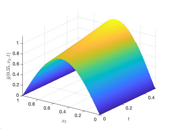
Figure 1: Projected uncontrolled state at $x_{1}=0.35$ and $x_{2}=0.4$.

In order to apply our results, let us define the appropariate weight functions. Suppose that the control region can be written in the following way:  $\omega=(a_{1},b_{1})\times(a_{2},b_{2})$, with $a_{i},b_{i}\in(0,1)$ and $a_{i}<b_{i}$, for $i=1,2$. For $s_{i}\in(0,1)$ with $i=1,2$, we consider the following real-valued function $\beta_{0,s_{i}}$:

$$\beta_{0,s_{i}}(x)=\dfrac{x(1-x)e^{-(x-c_{s_{i}})^{2}}}{s_{i}(1-s_{i})e^{-(s_{i}-c_{s_{i}})^{2}}},\quad c_{s_{i}}:=s_{i}-\dfrac{1-2s_{i}}{2s_{i}(1-s_{i})},\quad i=1,2.$$

Then, we set

$$\eta^{0}(x_{1},x_{2})=\beta_{0,s_{1}}(x_{1})\beta_{0,s_{2}}(x_{2})\quad\forall\,(x_{1},x_{2})\in\overline{\Omega}.$$ (6.2)

It is easy to check that $\eta^{0}$ fulfills the Fursikov-Imanuvilov conditions in (2.1). In the sequel, we define the weight functions $\rho$ and $\rho_{0}$ as in (2.2), with $\eta^{0}$ given by (6.2), $s_{i}=(b_{i}-a_{i})/2$ for $i=1,2$, $K_{1}=1/10$ and $K_{2}=2\|\eta^{0}\|_{L^{\infty}}=2$.

Several numerical experiments concerning (6.1) using ALG 3 are presented in the following sections. In all of them, ALG 3 is initiated with $q^{0}\equiv 0$ and the number of steps used for time discretization is denoted by $N_{t}$.

6.1 Test #1: Controlling with $\omega$ small enough

In this experiment, we consider the controlled heat equation where the action of the control is given in a small subset of the domain.

More precisely, in this case the control function in (6.1) is supported in the set $\omega=(0.2,0.5)\times(0.2,0.6)\subset\Omega$. Then, we use Uzawa’s algorithm proposed in ALG 3 with $R:=10^{5}$, $tol:=2\cdot 10^{-5}$, and $K=0.1$. We use an initial mesh with 2358 triangles and take $N_{t}=80$. We adapt the mesh every 10 iterates according to the values of

$$\tilde{y}^{k}(x):=\frac{1}{\Delta t}\sum_{n=0}^{N_{t}}y^{k}(x,t_{n}),\quad x\in\Omega.$$

where $t_{n}=n\Delta t$. In order to illustrate the evolution of the controlled solution, we have depicted the state $y=y(x_{1},x_{2},t)$ for some selected times in Figures 2 and  3. It is shown there that, as time evolves, the action of the control makes the computed solution locally negative; this is coherent with the Maximum Principle for the parabolic equation. Then, after a while, the solution tends rapidly to zero.

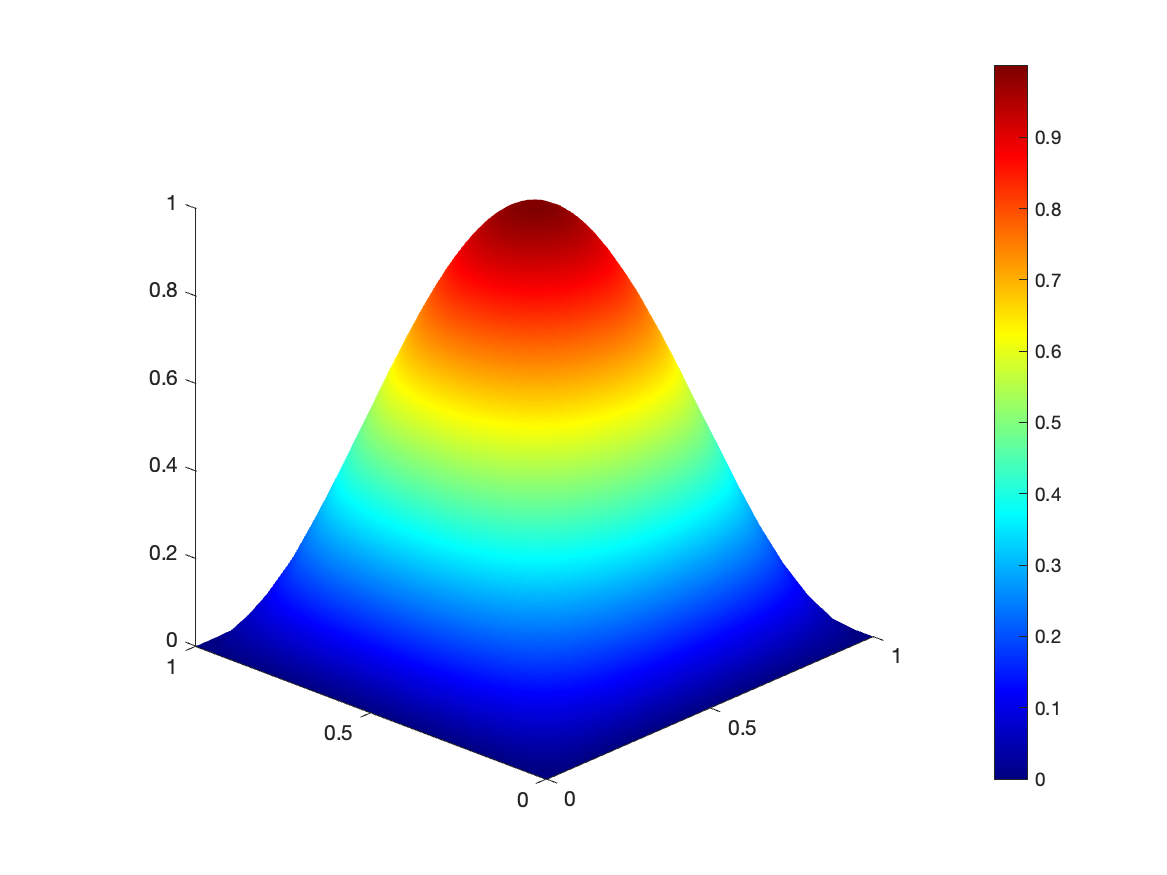
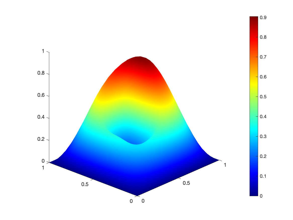
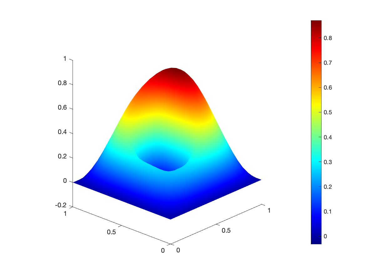
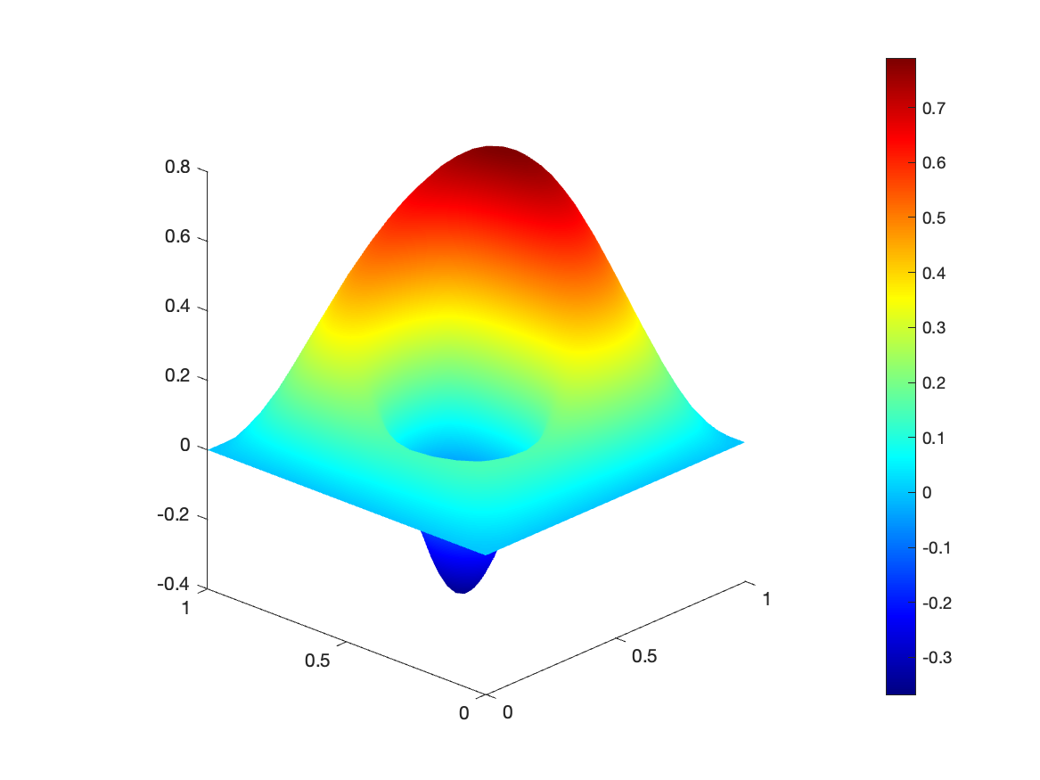
Figure 2: Evolution of the controlled state at $t=0,\,0.0625,\,0.0875$ and $0.15$ (From left to right).

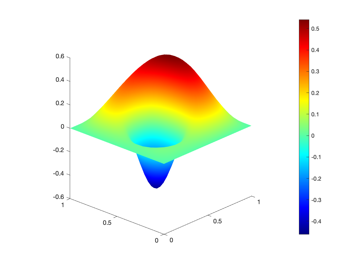
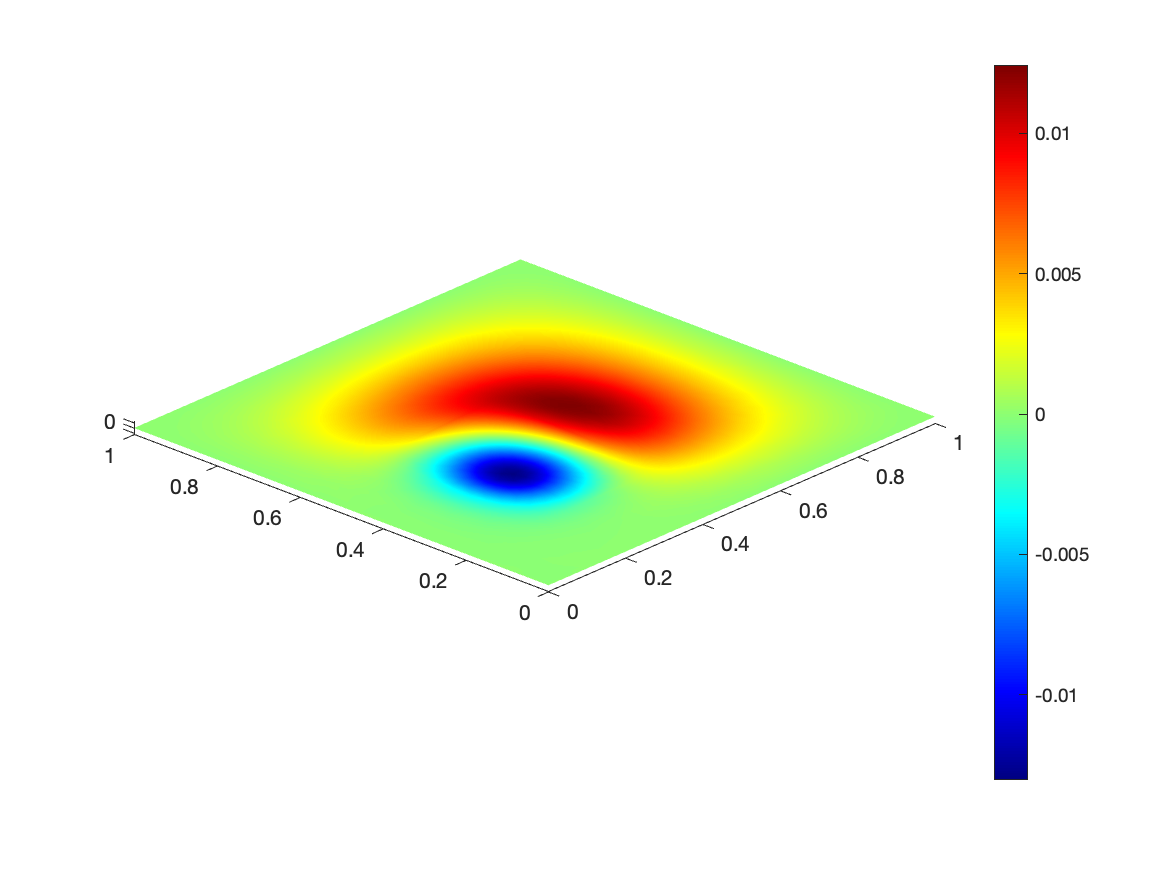
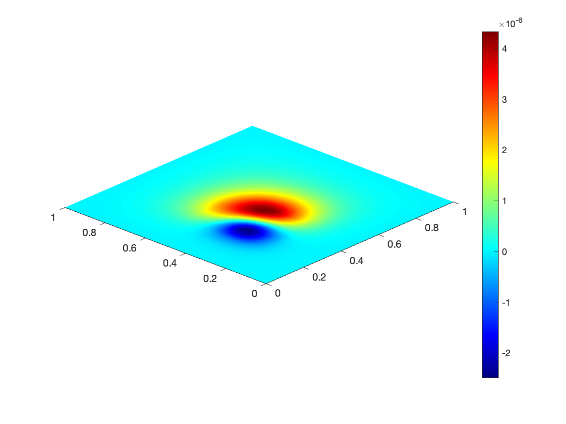
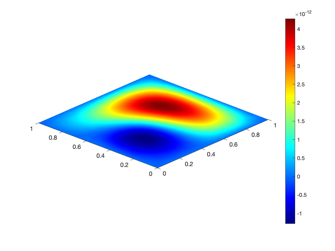
Figure 3: Evolution of the controlled state at $t=0.25,\,0.375,\,0.4375$ and $0.5$ (from left to right).

On the other hand, the projections of the control computed by ALG 3 at $x_{1}=0.35$ and then at $x_{2}=0.3$ are exhibited in Figure 4. We observe that, in Figure 4, the control takes positive values for some values of $t$ close to the final time. Again, this is coherent with the Maximum Principle for the heat equation.

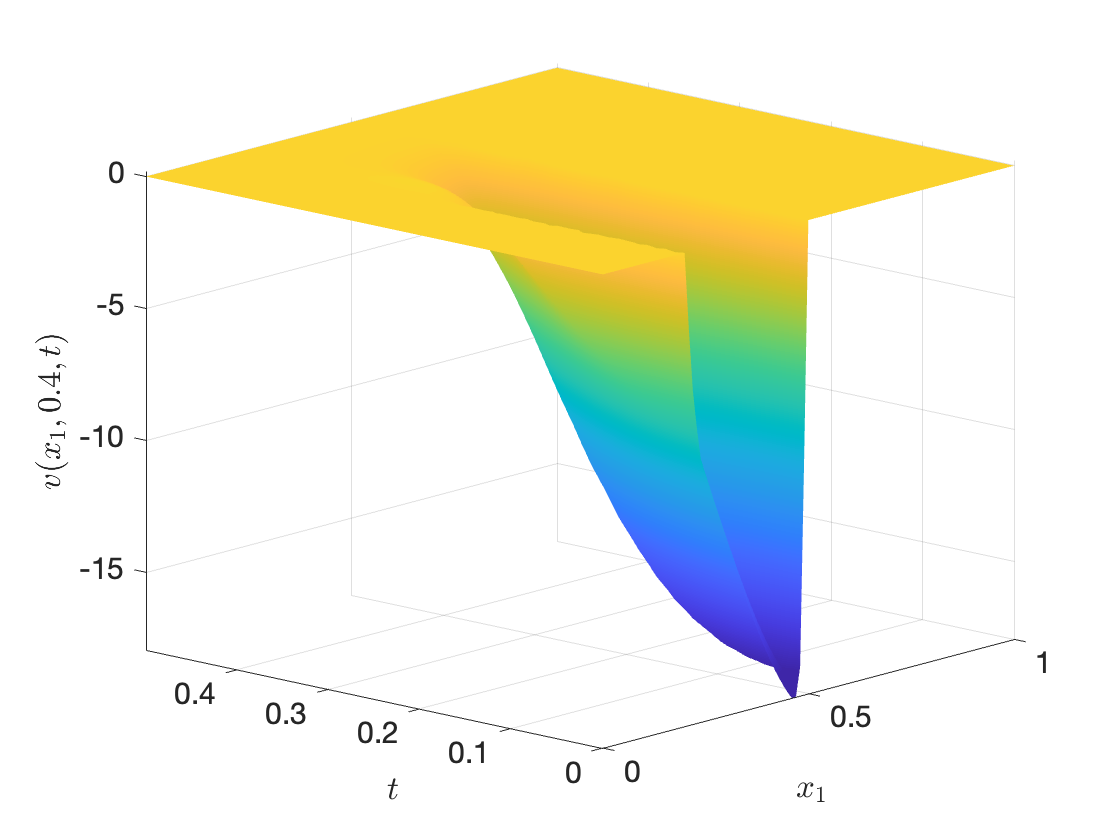
Figure 4: Projected uncontrolled state at $x_{1}=0.35$ (left) and $x_{2}=0.4$ (right).

The norms of $y$ and $q$ at final time $T$ are given by

$$\|y(\cdot\,,T)\|_{L^{2}(\Omega)}=1.71997\cdot 10^{-12},\quad\|q(\cdot\,,T)\|_{L^{2}(\Omega)}=35.0714.$$

For the evolution of the spatial norms of the uncontrolled and controlled states, the control and the computed $q$, see Figures 5 and 6. Note that the norm of the controlled state decays exponentially as $t\to T^{-}$.

The initial and final meshes obtained by the adapt mesh procedure used for the computations can be seen in Figure 7. Observe that they contain $2358$ and $1899$ triangles, respectively.

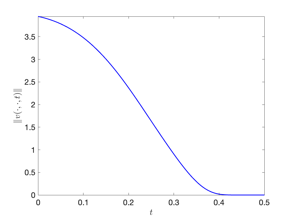
Figure 5: The evolution of $\|\bar{y}(\cdot\,,t)\|_{L^{2}}$ and $\|y(\cdot\,,t)\|_{L^{2}}$ (left) and the evolution of $\|v(\cdot\,,t)\|_{L^{2}(\omega)}$ (right) as $t\in[0,T]$.

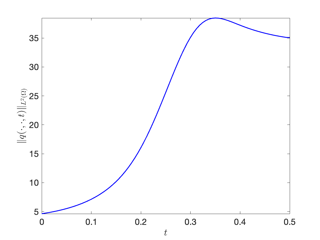
Figure 6: The evolution of $\|q(\cdot\,,t)\|_{L^{2}}$ with $t\in[0,T]$.

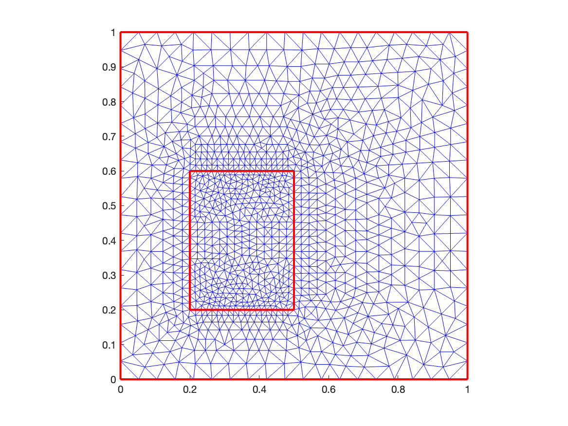
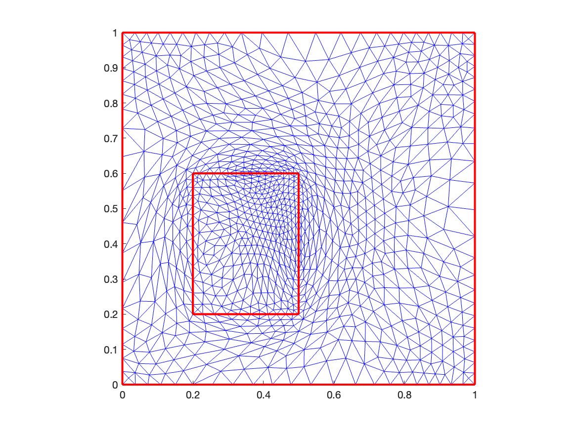
Figure 7: The initial(left) and final(right) meshes.

6.2 Test #2: The behavior of the state and the control as $R\to\infty$ for ALG 3

Let us fix $\omega=(0.2,0.8)\times(0.2,0.8)$, $T=0.5$ and $N_{t}=20$ and let us consider the corresponding system (6.1). We report the performance obtained by ALG 3 with $K=0.1$ by using different values of $R$ and adapting the mesh each $10$ iterates.

In Table 1, we give details on the behavior of the norms of $y$, $v$, $q$, $y(\cdot\,,T)$ and $q(\cdot\,,T)$ with respect to $R$. We observe that $R$ has a weak influence on the $L^{2}$-norms of $y$ and $v$. This confirms that, as $R$ increases, we get the uniform convergence of the state and the control. The same happens to the $L^{2}$-norm of $q$ and the norm in $L^{2}(\Omega)$ of $q(\cdot\,,T)$.

On the other hand, the norm of $\|y(\cdot\,,T)\|_{L^{2}}$ strongly depends on $R$ and we see that it tends to 0 as $R\to\infty$ in practice proportionally to $1/R$.

$R$	$\|y\|_{L^{2}(Q)}$	$\|v\|_{L^{2}(Q_{\omega})}$	$\|q\|_{L^{2}(Q)}$	$\|y(\cdot\,,T)\|_{L^{2}(\Omega)}$	$\|q(\cdot\,,T)\|_{L^{2}(\Omega)}$
$10^{3}$	$0.155245$	$1.47251$	$24.1339$	$1.33195\times 10^{-9}$	$8.55816$
$10^{4}$	$0.155226$	$1.47274$	$24.1122$	$1.32407\times 10^{-11}$	$8.52156$
$10^{5}$	$0.155262$	$1.47354$	$24.1811$	$1.319610^{-13}$	$8.62848$
$10^{6}$	$0.155224$	$1.47355$	$24.1381$	$1.31352\times 10^{-15}$	$8.57142$
$10^{7}$	$0.155211$	$1.47368$	$24.138$	$1.4735\times 10^{-17}$	$8.60645$
$10^{8}$	$0.155186$	$1.47416$	$24.14$	$3.40873\times 10^{-19}$	$8.60533$

Table 1: The values of the norms of $y$, $v$, $q$, $y(\cdot\,,T)$ and $q(\cdot\,,T)$ as $R$ increases.

The number of iterates needed to achieve

$$\dfrac{\|q^{k+1}-q^{k}\|_{L^{2}(Q)}}{\|q^{k}\|_{L^{2}(Q)}}\leqslant tol:=1\cdot 10^{-5}$$ (6.3)

and the numbers of vertices and triangles in the final meshes are furnished in Table 2.

$R$	$\#$ iterates	$\#$ vertices	$\#$ triangles
$10^{3}$	$3035$	$1146$	$2154$
$10^{4}$	$3037$	$1148$	$2159$
$10^{5}$	$3028$	$1151$	$2166$
$10^{6}$	$3030$	$1149$	$2160$
$10^{7}$	$3026$	$1155$	$2174$
$10^{8}$	$3025$	$1149$	$2161$

Table 2: The number of iterates, vertices, and needed triangles as $R$ increases.

We observe that these values remain stable as $R$ increases. This indicates that ALG 3 behaves robustly “with respect to truncation”. Moreover, we observe that the huge number of iterates to achieve (6.3) is similar to those obtained by the conjugate gradient method applied in [8] due to the lack of uniform coercivity of the dual problem.

Tables 1 and 2 suggest that it is not necessary to take $R\to+\infty$ to achieve a good approximation of the controls. In fact, thanks to the use of the weight functions $\rho_{R}$ and $\rho_{0}$, the norms of the computed controls and controlled states change only slightly concerning these parameters. Moreover, in contrast to the case of conjugate gradient algorithm, we do not have a significative increase of iterates when $R$ increases.

6.3 Test #3: Influence of the weights

Let us take $\omega=(0.2,0.8)\times(0.2,0.8)$ and $T=0.5$ and consider again the controlled problem (6.1). We apply again ALG 3 with $K=0.1$, $R=10^{5}$, $q^{0}\equiv 0$, adapting the spatial mesh every 10 iterates. In this case, the stopping criteria is as (6.3) with $tol=10^{-4}$.

In Tables 3 and 4, the behavior of the algorithm is shown for various values of $N_{t}$.

$N_{t}$	$\|y\|_{L^{2}(Q)}$	$\|v\|_{L^{2}(Q_{\omega})}$	$\|q\|_{L^{2}(Q)}$	$\|y(\cdot\,,T)\|_{L^{2}}$	$\|q(\cdot\,,T)\|_{L^{2}}$
20	0.156718	1.17555	5.3525	$2.63373\cdot 10^{-13}$	6.18708
40	0.150623	1.1082	4.29809	$2.78415\cdot 10^{-13}$	5.84151
60	0.147944	1.08737	3.97457	$2.96496\cdot 10^{-13}$	5.7084
80	0.146301	1.07509	3.81718	$3.14825\cdot 10^{-13}$	5.6242
100	0.145286	1.06806	3.73284	$3.28547\cdot 10^{-13}$	5.5786
120	0.144542	1.06397	3.68143	$3.36813\cdot 10^{-13}$	5.55647
160	0.143917	1.06091	3.63826	$3.38874\cdot 10^{-13}$	5.52634
200	0.142921	1.05326	3.57356	$3.61723\cdot 10^{-13}$	5.48535

Table 3: The norms of $y$, $v$, $q$, $y(\cdot\,,T)$ and $q(\cdot\,,T)$ as $N_{t}$ increases.

$N_{t}$	#iterates	#vertices	#triangles
20	462	887	1657
40	379	861	1608
60	342	840	1569
80	321	827	1544
100	309	813	1518
120	301	803	1497
160	294	801	1494
200	284	792	1478

Table 4: The number of iterates, vertices, and triangles of the final mesh when $N_{t}$ increases.

In particular, the uniform convergence of the control and the controlled state is clear. Moreover, the control functions approximate satisfactorily the null controllability requirement, since in each case $\|y(\cdot\,,T)\|_{L^{2}}\sim 10^{-13}$. The number of iterates is slightly reduced when $N_{t}$ increases and the final mesh obtained in each case remains without significative changes.

To end the experiments for the 2D heat equation using ALG3, we study the evolution of the $\log_{10}$ scale of the relative error to achieve the condition

$$\dfrac{\|q^{k+1}-q^{k}\|_{L^{2}(Q)}}{\|q^{k}\|_{L^{2}(Q)}}\leqslant 10^{-6}.$$

This is displayed in the Figure 8.

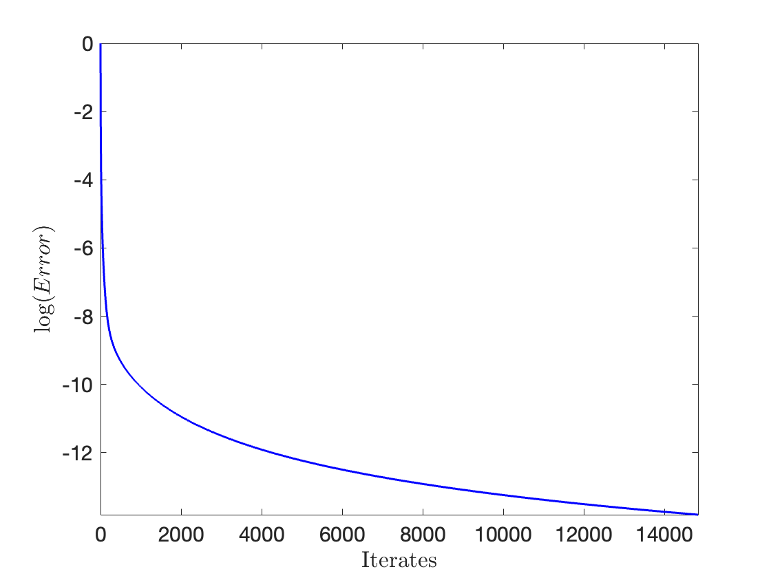
Figure 8: Iterates vs Logarithm of the relative error.

We thus see that the evolution of the relative error is nonlinear with respect to the number of iterates, a usual phenomenon in ill-posed parabolic problems. To be more precise, the slope of the curve reduces significantly after the first 200 iterates.

6.4 Test #4: An experiment for a $3$D heat equation

Now, we consider the $3$D domain $\Omega=[0,1]^{3}$ and the control region $\omega=[0.2,0.4]^{3}$, we fix $T=0.5$ and we deal with the (controlled) heat equation (1.1) with $a=0.01$, $b=-1.0$ and the initial condition

$$y^{0}(x_{1},x_{2},x_{3})=100\cdot\sin(\pi x_{1})\,\sin(\pi x_{2})\,\sin(\pi x_{3})\quad\forall(x_{1},x_{2},x_{3})\in\Omega.$$

We also consider a 3D version of the function $\eta^{0}$ given by (6.2) and set the functions $\rho$ and $\rho_{0}$ accordingly. The goal is to solve the extremal problem (1.4).

We consider a 3D mesh whose numbers of tetrahedrons and vertices are, respectively, $11023$ and $2042$; see Figure 9.

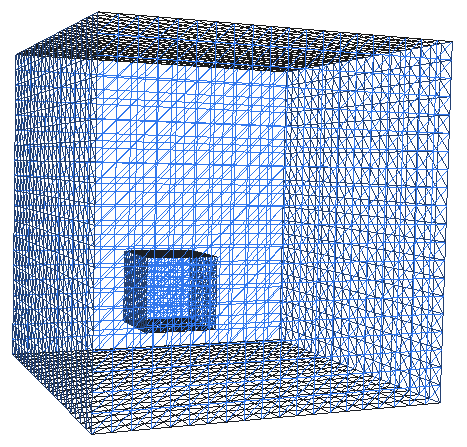
Figure 9: 3D mesh with $\#t=11023$ and $\#v=2042$.

We use ALG 3 to solve the null controllability problem. The stopping criteria is

$$\dfrac{\|q^{k+1}-q^{k}\|_{L^{2}(Q)}}{\|q^{k}\|_{L^{2}(Q)}}\leqslant 10^{-5}.$$

The computed controlled solution can be found in Figure 10 at several times. On the other hand, the projected controlled state and the projected associated control at $x_{1}=x_{2}=0.3$ are given in Figures 12 and 12.

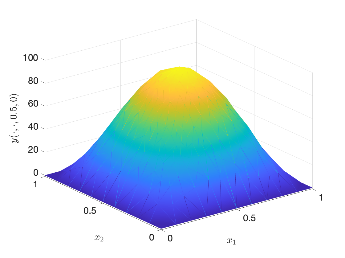
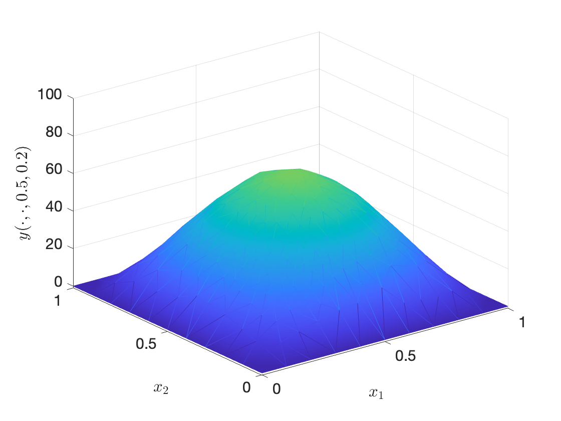
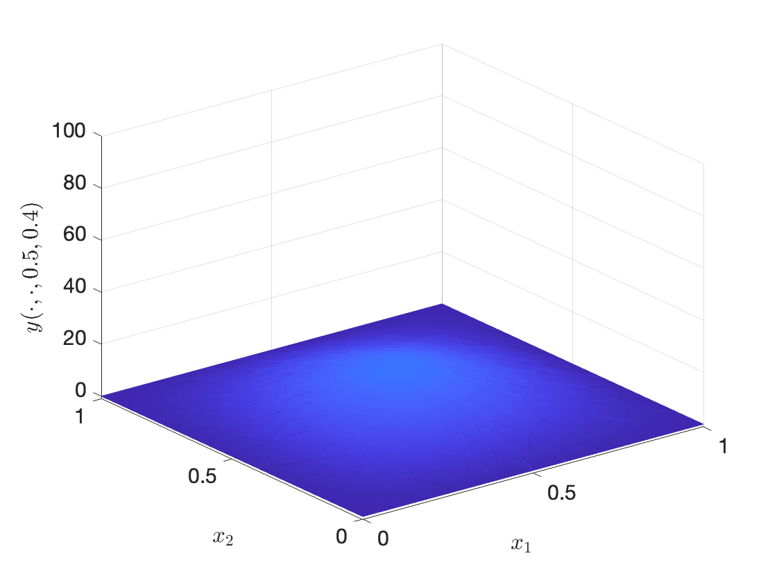
Figure 10: Evolution of the computed state at $t=0$ (left), $0.2$ (center) and $0.4$ (right).

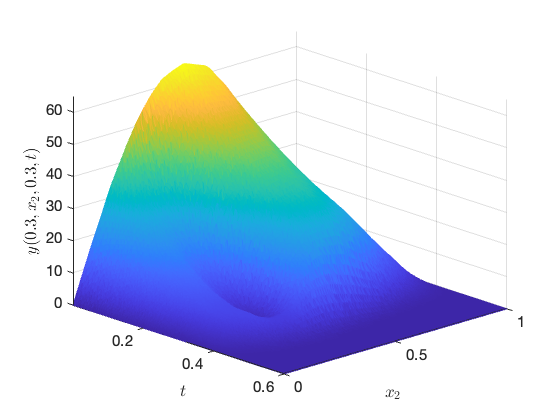
Figure 11: The projected state ($x_{1}\!=\!x_{3}\!=\!0.3$).

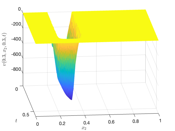
Figure 12: The projected control ($x_{1}\!=\!x_{3}\!=\!0.3$).

In addition, we have

$$\|y(\cdot\,,T)\|_{L^{2}}=2.09824\cdot 10^{-7}\text{ and }\|q(\cdot\,,T)\|_{L^{2}}=45.8320.$$

The evolution in time of $\|\bar{y}(\cdot\,,t)\|_{L^{2}}$, $\|y(\cdot\,,t)\|_{L^{2}}$ and $\|v(\cdot\,,t)\|_{L^{2}(\omega)}$ are depicted in Figures 14 and 14. In addition, the evolution in time of $\|q(\cdot\,,t)\|_{L^{2}}$ is presented in Figure 15.

Figure 13: $\|\bar{y}(\cdot\,,t)\|_{L^{2}}$ and $\|y(\cdot\,,t)\|_{L^{2}}$.

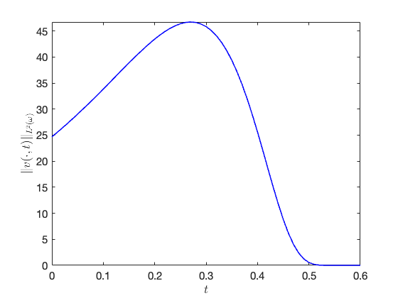
Figure 14: Evolution of $\|v\|_{L^{2}(Q_{\omega})}$.

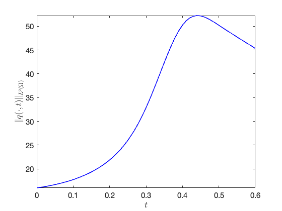
Figure 15: Evolution of $\|q\|_{L^{2}(Q)}$.

6.5 Test #5: An experiment for the $2$D Stokes system

In this experiment, we take $\Omega=(0,1)^{2}\subset\mathbb{R}^{2}$, $\omega=(0.2,0.4)^{2}$ and $T=0.6$. We consider the problem (5.1) with $a=0.05$,

$$\bm{x}=\left(\begin{array}[]{c}x_{1}\\ x_{2}\end{array}\right),\quad\bm{y}=\left(\begin{array}[]{c}y_{1}\\ y_{2}\end{array}\right),\quad\bm{v}=\left(\begin{array}[]{c}v_{1}\\ v_{2}\end{array}\right),$$

with the initial condition

$$\bm{y}^{0}(\bm{x})=10^{3}\left(\begin{array}[]{c}x_{1}^{2}(1-x_{1})^{2}x_{2}(1-x_{2})^{2}\\ -x_{1}(1-x_{1})(0.5-2x_{1})x_{2}^{2}(1-x_{2})^{2}.\end{array}\right).$$

We consider a mesh with $1698$ triangles and $878$ vertices (see Figure 16).

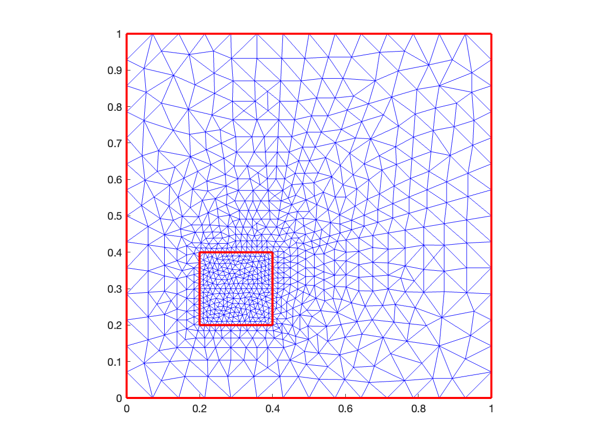
Figure 16: Mesh with 1698 triangles and 878 vertices.

The uncontrolled solution of the Stokes system is depicted in Figure 17. We note that the solution does not vanish at $t=T$. We apply ALG 3 with $K=0.1$, $R=10^{5}$ and stopping criteria

$$\frac{\|\bm{q}^{k+1}-\bm{q}^{k}\|_{\bm{L}^{2}(Q)}}{\|\bm{q}^{k}\|_{\bm{L}^{2}(Q)}}\leqslant 1\cdot 10^{-5}.$$

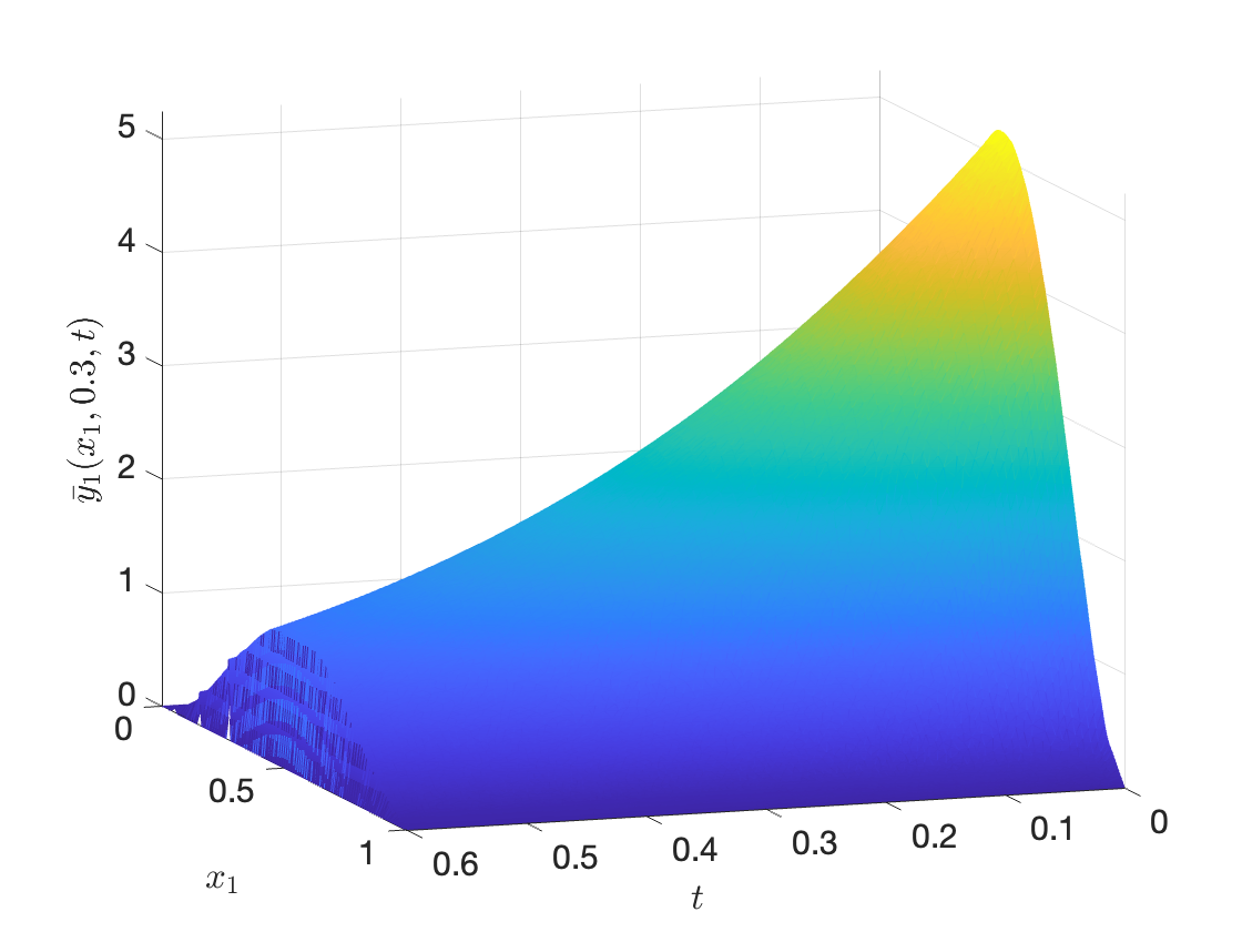
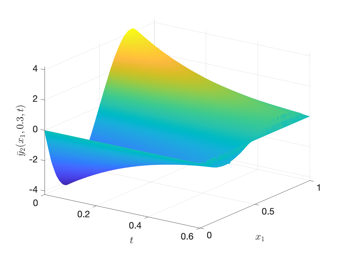
Figure 17: The $x_{1}$-projected first(left) and second(right) component of the uncontrolled solution at $x_{2}=0.3$.

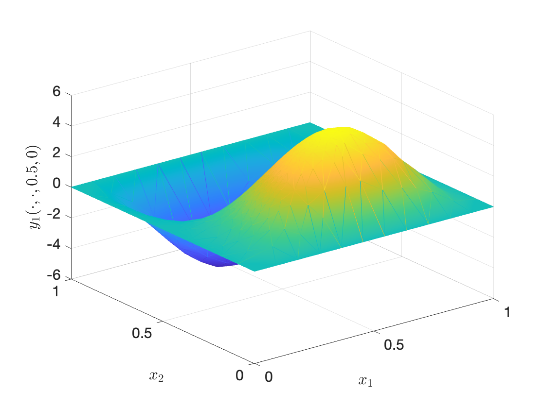
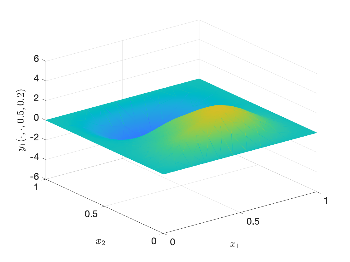
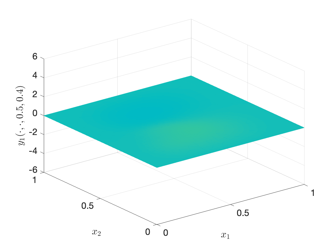
Figure 18: The projected controlled solution component $y_{1}$ in at $t=0$(left), $t=0.2$(center) and $t=0.4$(right).

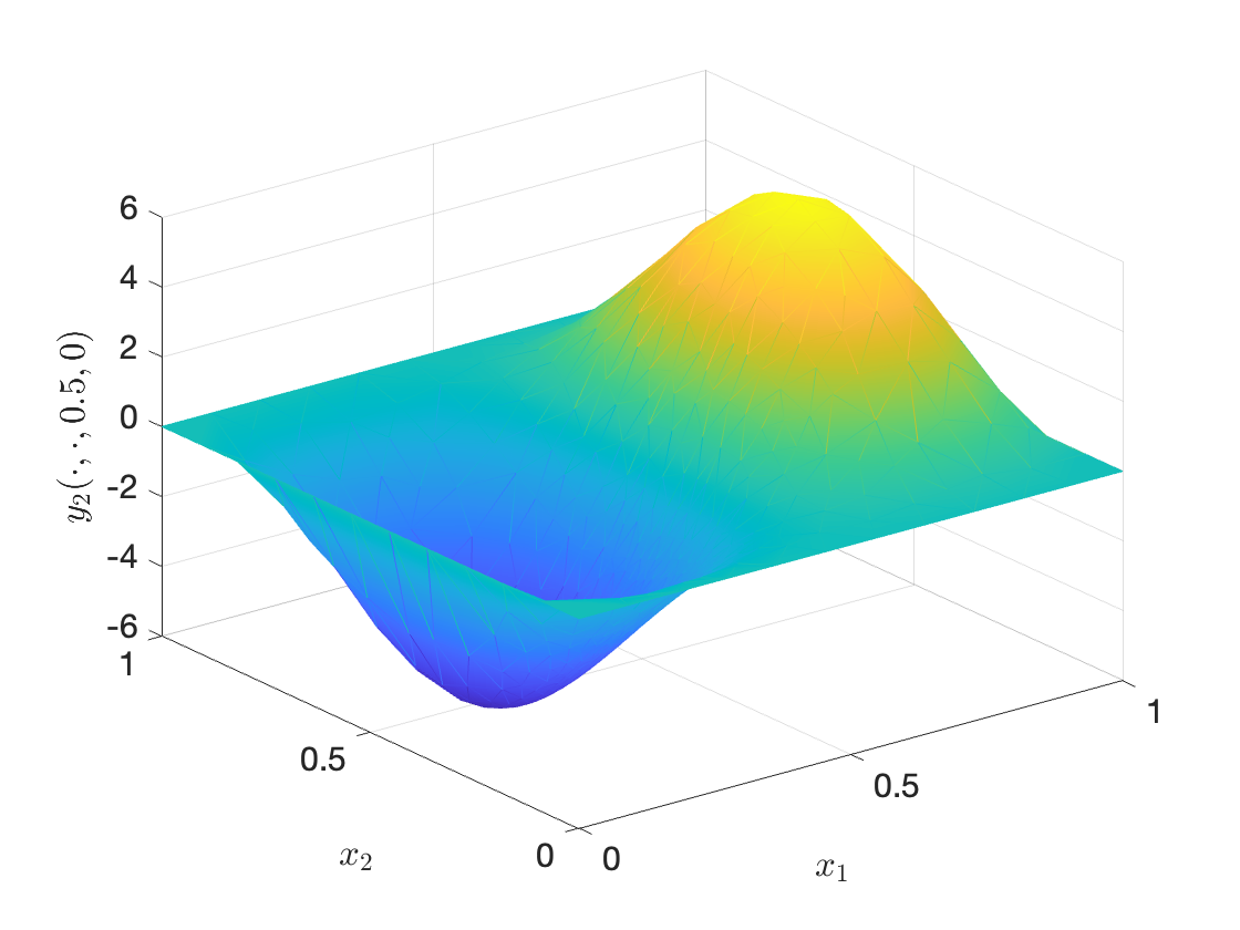
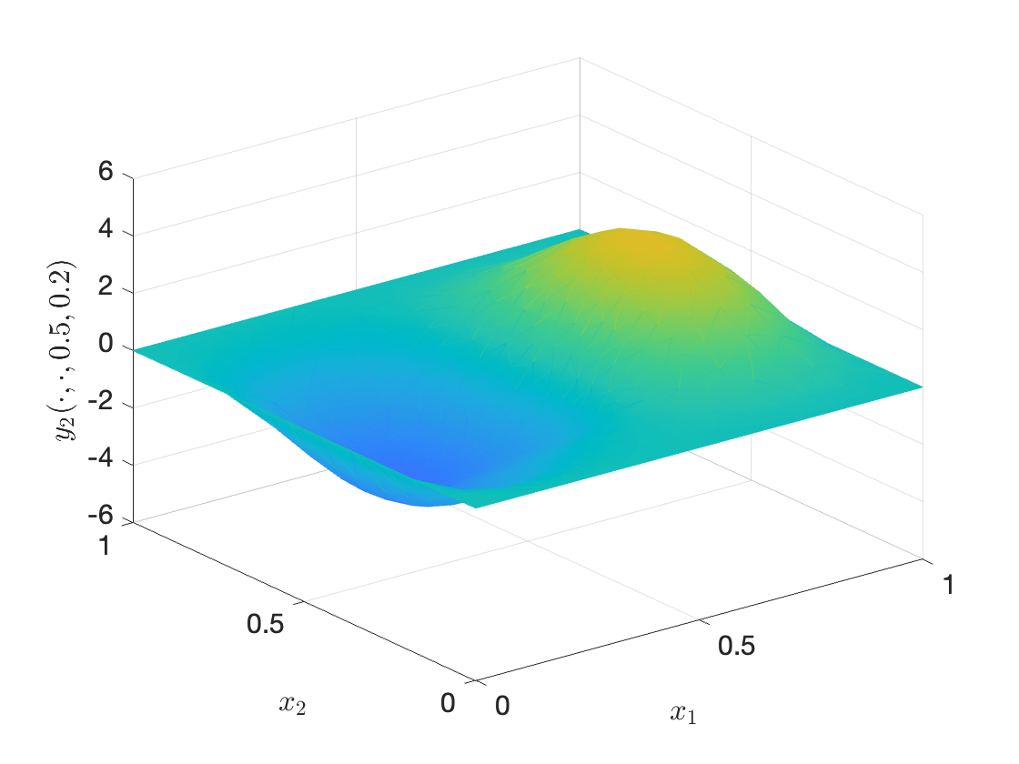
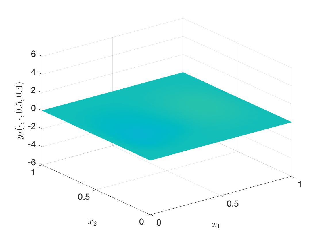
Figure 19: The projected controlled solution component $y_{2}$ in at $t=0$(left), $t=0.2$(center) and $t=0.4$(right).

The components of the projected state are given in Figures 18 and 19. We observe there that the solution vanishes at $t=T$. In fact, the norms of the controlled state and $\bm{q}$ at $t=T$ are given by

$$\|\bm{y}(\cdot\,,T)\|_{L^{2}}=5.50185\times 10^{-9}\text{ and }\|\bm{q}(\cdot\,,T)\|_{L^{2}}=55.0852.$$

The components of the projected control are depicted in Figures 21 and 21.

The evolution in time of the norms of $\bar{\bm{y}}$, $\bm{y}$ and $\bm{v}$ is given in Figures 23 and 23. In addition, the evolution of $\|\bm{q}(\cdot\,,t)\|_{L^{2}}$ is shown in Figure 24.

Once more, we observe in Figures 23 and 23 that the norms of the state and the control go to zero as $t\to T^{-}$.

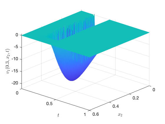
Figure 20: The projected $v_{1}$.

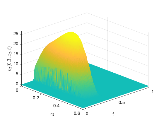
Figure 21: The projected $v_{2}$.

Figure 22: The $L^{2}$-norms of $\bm{y}(\cdot,t)$ and $\bm{\overline{y}}(\cdot,t)$.

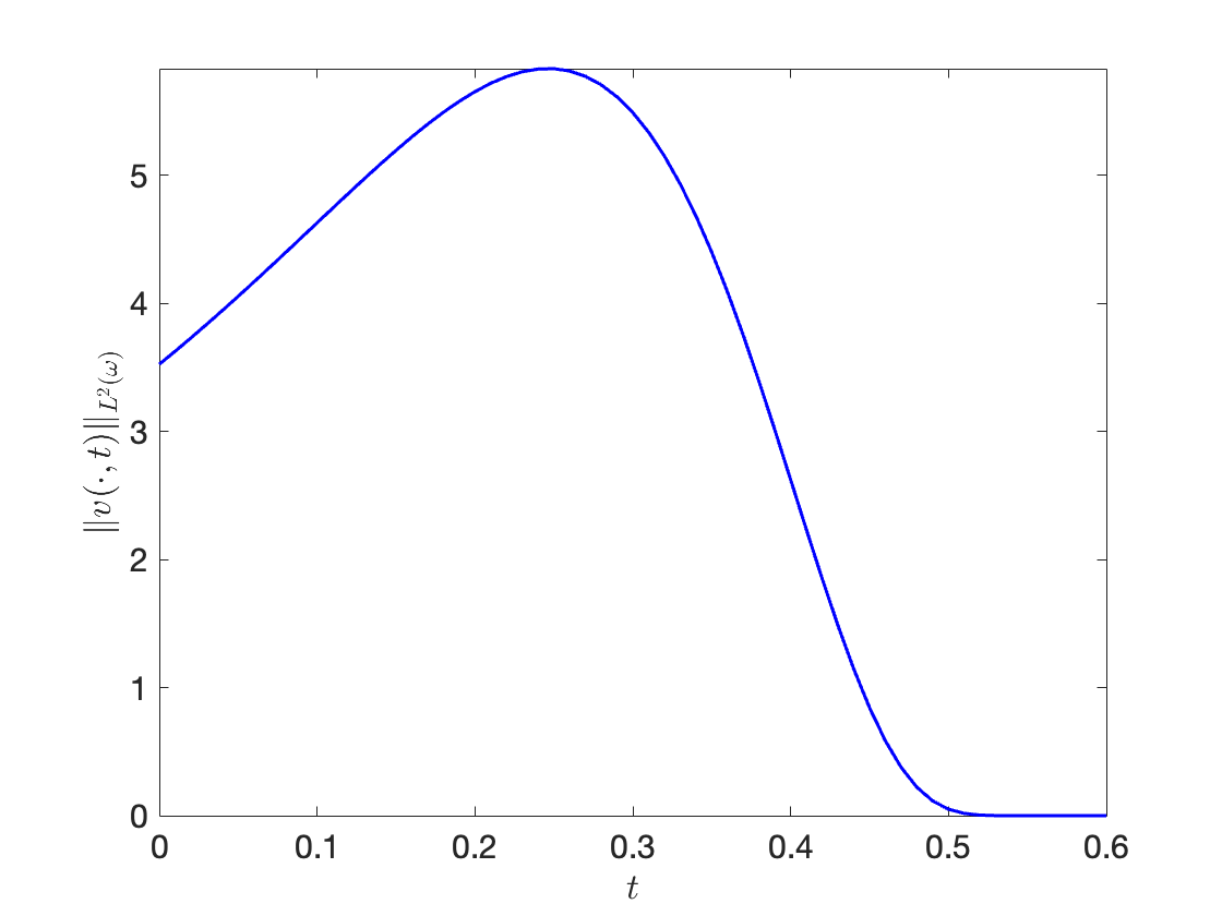
Figure 23: The $L^{2}$-norm of $\bm{v}(\cdot,t)$

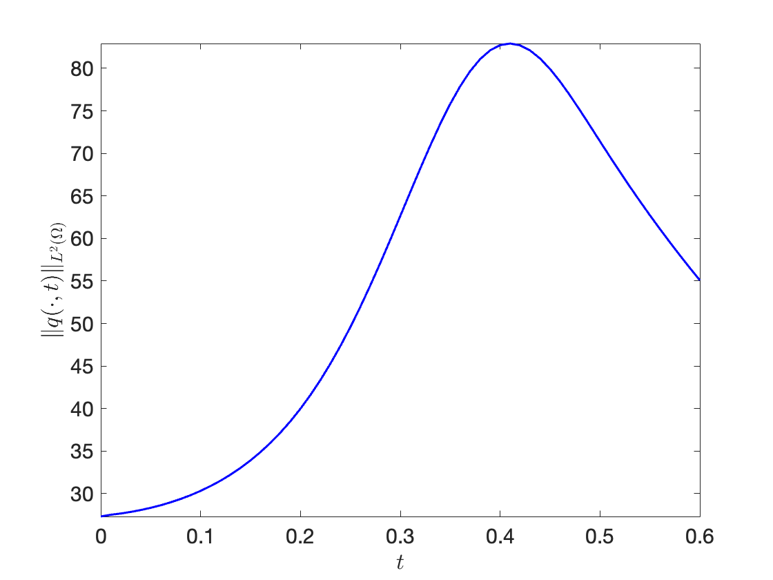
Figure 24: $\|\bm{q}(\cdot\,,t)\|_{\bm{L}^{2}(\omega)}$.

7 Summary and further comments

In this paper, we have presented several algorithms based on Lagrangian and Augmented Lagrangian formulations of null controllability problems for the heat and the Stokes PDEs. To apply the techniques, we introduced a large parameter $R>0$ in order to truncate the weight function associated with the state variable and then a second paremater $K>0$ that plays the role of penalization in the Augmented Lagrangian. As $R$ goes to $+\infty$, we recover the solution of the original problem. This is proved rigorously and has been numerically validated in several experiments.

One of the main virtues of the presented methods is that it can be applied with reasonable effort to control problems for high spatial dimension PDEs, which is not so clear for other strategies.

The arguments and results can be extended and adapted to many other controllability problems. Thus, they are valid for the internal or boundary control of parabolic PDEs and systems complemented with other boundary conditions, control problems in other domains, etc.

In a next future, we will investigate their utility in the context of some semilinear and nonlinear problems like state-dependent diffusion heat equations, Burgers, Navier-Stokes, and Boussinesq systems, etc.

The formulation and resolution of null or exact controllability problems with Lagrangian and Augmented Lagrangian methods for wave and Schrödinger PDEs remain, as far as we know, unexplored. This will also be investigated in forthcoming work.

References

• [1] D. Allonsius and F. Boyer. Boundary null-controllability of semi-discrete coupled parabolic systems in some multi-dimensional geometries. Math. Control Relat. Fields, 10(2):217–256, 2020.
• [2] F. Boyer. On the penalised HUM approach and its applications to the numerical approximation of null-controls for parabolic problems. In CANUM 2012, 41e Congrès National d’Analyse Numérique, volume 41 of ESAIM Proc., pages 15–58. EDP Sci., Les Ulis, 2013.
• [3] C. Carthel, R. Glowinski, and J.-L. Lions. On exact and approximate boundary controllabilities for the heat equation: a numerical approach. J. Optim. Theory Appl., 82(3):429–484, 1994.
• [4] J.-M. Coron. Control and nonlinearity, volume 136 of Mathematical Surveys and Monographs. American Mathematical Society, Providence, RI, 2007.
• [5] I. Ekeland and R. Témam. Convex analysis and variational problems, volume 28 of Classics in Applied Mathematics. Society for Industrial and Applied Mathematics (SIAM), Philadelphia, PA, english edition, 1999. Translated from the French.
• [6] E. Fernández-Cara and S. Guerrero. Global Carleman inequalities for parabolic systems and applications to controllability. SIAM J. Control Optim., 45(4):1399–1446, 2006.
• [7] E. Fernández-Cara and A. Münch. Strong convergent approximations of null controls for the 1D heat equation. SeMA J., 61:49–78, 2013.
• [8] E. Fernández-Cara and A. Münch. Numerical exact controllability of the 1D heat equation: duality and Carleman weights. J. Optim. Theory Appl., 163(1):253–285, 2014.
• [9] M. Fortin and R. Glowinski. Augmented Lagrangian methods, volume 15 of Studies in Mathematics and its Applications. North-Holland Publishing Co., Amsterdam, 1983. Applications to the numerical solution of boundary value problems, Translated from the French by B. Hunt and D. C. Spicer.
• [10] A. V. Fursikov and O. Yu. Imanuvilov. Controllability of evolution equations, volume 34 of Lecture Notes Series. Seoul National University, Research Institute of Mathematics, Global Analysis Research Center, Seoul, 1996.
• [11] R. Glowinski and J.-L. Lions. Exact and approximate controllability for distributed parameter systems. In Acta numerica, 1995, Acta Numer., pages 159–333. Cambridge Univ. Press, Cambridge, 1995.
• [12] R. Glowinski, J.-L. Lions, and J. He. Exact and approximate controllability for distributed parameter systems, volume 117 of Encyclopedia of Mathematics and its Applications. Cambridge University Press, Cambridge, 2008. A numerical approach.
• [13] F. Hecht. New development in freefem++. J. Numer. Math., 20(3-4):251–265, 2012.
• [14] I. Lasiecka and R. Triggiani. Control theory for partial differential equations: continuous and approximation theories. I, volume 74 of Encyclopedia of Mathematics and its Applications. Cambridge University Press, Cambridge, 2000. Abstract parabolic systems.
• [15] I. Lasiecka and R. Triggiani. Control theory for partial differential equations: continuous and approximation theories. II, volume 75 of Encyclopedia of Mathematics and its Applications. Cambridge University Press, Cambridge, 2000. Abstract hyperbolic-like systems over a finite time horizon.
• [16] G. Lebeau and L. Robbiano. Contrôle exact de l’équation de la chaleur. Comm. Partial Differential Equations, 20(1-2):335–356, 1995.
• [17] P. Martin, L. Rosier, and P. Rouchon. Null controllability of the heat equation using flatness. Automatica J. IFAC, 50(12):3067–3076, 2014.
• [18] P. Martin, L. Rosier, and P. Rouchon. Null controllability of one-dimensional parabolic equations by the flatness approach. SIAM J. Control Optim., 54(1):198–220, 2016.
• [19] P. Martin, L. Rosier, and P. Rouchon. Controllability of parabolic equations by the flatness approach. In Evolution equations: long time behavior and control, volume 439 of London Math. Soc. Lecture Note Ser., pages 161–178. Cambridge Univ. Press, Cambridge, 2018.
• [20] S. Micu and E. Zuazua. On the regularity of null-controls of the linear 1-d heat equation. C. R. Math. Acad. Sci. Paris, 349(11-12):673–677, 2011.
• [21] A. Münch and E. Zuazua. Numerical approximation of null controls for the heat equation: ill-posedness and remedies. Inverse Problems, 26(8):085018, 39, 2010.
• [22] D. L. Russell. Controllability and stabilizability theory for linear partial differential equations: recent progress and open questions. SIAM Rev., 20(4):639–739, 1978.