The imaginary-$\theta$ dependence of the SU($N$) spectrum

Abstract

In this talk we will report on a study of the $\theta$-dependence of the string tension and of the mass gap of four-dimensional SU($N$) Yang–Mills theories. The spectrum at $N=3$ and $N=6$ was obtained on the lattice at various imaginary values of the $\theta$-parameter, using Parallel Tempering on Boundary Conditions to avoid topological freezing at fine lattice spacings. The coefficient of the $\mathcal{O}(\theta^{2})$ term in the Taylor expansion of the spectrum around $\theta=0$ could be obtained in the continuum limit for $N=3$, and on two fairly fine lattices for $N=6$.

1 Introduction

The study of systems described by a Yang-Mills (YM) action augmented with a $\theta$-term has provided, historically, several interesting results. Classically speaking, the addition of a $\theta$-term does not alter the classical equations of motion. Yet, its theoretical and phenomenological implications are far reaching, once the quantum fluctuations are taken into account. The $\theta$-dependence lies at the heart of the Witten–Veneziano solution of the $\eta$-$\eta^{\prime}$ puzzle [1, 2, 3, 4] and it is the starting point for the Peccei–Quinn hypothetical solution to the strong-CP problem based on axions. Accordingly, the study of $\theta$-dependence in a variety of different settings has attracted a great deal of attention in the past years. Starting from QCD, SU($N$) and Sp($2N$) models [5, 6, 7] in $4d$, to $CP^{N-1}$ models [8, 9] and U(N) models [10, 11, 12] in $2d$, to quantum mechanical models [13, 14, 15].

So far, the main target of investigation has been the free energy of the system and its $\theta$-dependence, both at zero and finite temperature. Using analytical methods, it is possible to obtain theoretical predictions for the $\theta$-dependence of the QCD vacuum energy either using effective theories close to the chiral limits for low temperatures [16, 17, 18, 19], where the $\theta$-dependence of the vacuum energy essentially stems from the $\theta$-dependence of the pion mass (the $\theta$-dependence of the mass of some light resonances has also been investigated in [20]); or for the $\theta$-dependence of the QCD free energy via perturbative and semi-classical arguments for asymptotically-high temperatures [6, 7, 21]. Away from these regimes, the $\theta$-dependence of the vacuum energy has been investigated by means of numerical Monte Carlo simulations of the lattice-discretized theory, both in QCD [22, 23, 24, 25, 26, 27, 28, 29] and in $\mathrm{SU}(N)$ pure-gauge theories [30, 31, 32, 33, 34, 35, 36, 37, 38, 39, 40, 41, 42, 43, 44, 45, 46, 47], with particular focus on the large-$N$ limit of these models, due to its relation with the Witten–Veneziano mechanism [1, 2, 3, 4].
Concerning two-dimensional models, the $\theta$-dependence of $2d$ $\mathrm{CP}^{N-1}$ models is amenable to be exactly computed using analytical methods in the large-$N$ limit up to the next-to-leading-order in the $1/N$ expansion [8, 48, 49, 50, 45], and such predictions have been verified to be supported by numerical evidence [51, 52, 53, 12, 11]. The $\theta$-dependence of $2d$ $\mathrm{CP}^{N-1}$ models has also been studied numerically [54, 55] in the limit $N\to 2$, as these theories reduce to the $2d$ O(3) non-linear $\sigma$ model in this limit (see also [56, 57]), whose $\theta$-dependence is theoretically interesting due to its connection with the Haldane conjecture. Finally, also the $\theta$-dependence of $2d$ $\mathrm{U}(N)$ Yang–Mills theories can be exactly computed analytically [10, 11, 12].

The $\theta$-dependence of the spectrum of the theory has received comparatively less attention, with only one exploratory lattice study [49] present in the literature. Our main goal is to bridge that gap. In particular, we report on our study [58] of the $\theta$-dependence of the spectrum of glueballs and fluxtubes of pure-gauge $\mathrm{SU}(N)$ models in $4d$. The results that we have obtained constitute a substantial improvement over the previously available results. This could be achieved with the combination of the imaginary-$\theta$ method and of the Parallel Tempering on Boundary Conditions (PTBC) algorithm. The former enables us to improve the signal-to-noise ratio compared to the standard Taylor expansion approach, and the latter enabled us to avoid the freezing of topology, especially at large-$N$.

This proceeding is organized as follows. In Sec. 2 we describe our numerical setup. In Sec. 3 we present the main results of [58]. Finally, in Sec. 4 we draw our conclusions.

2 Numerical Setup

Direct lattice simulations of the Yang–Mills theory at non-zero values of $\theta$ are hindered by the infamous sign problem, as the topological term is purely imaginary, thus yielding a complex action. A popular technique to bypass the sign-problem is to resort to simulations of imaginary-values of $\theta_{{}_{\scriptscriptstyle{\mathrm{I}}}}\equiv\mathrm{i}\theta$, characterized by a purely-real action. Assuming analyticity around $\theta=0$ it is possible to use analytic continuation and infer the dependence on the real parameter $\theta$ from the observed dependence on the imaginary one $\theta_{{}_{\scriptscriptstyle{\mathrm{I}}}}$, at least for small enough values of $\theta$. The imaginary-$\theta$ method has been shown to be extremely effective in improving the signal-to-noise-ratio of the higher-order coefficients in the $\theta$-expansion of several quantities, compared to simulations at $\theta=0$ alone [59, 60, 61, 62, 63, 38, 57, 64, 65, 44, 45, 46, 47, 52, 53, 66, 67]. Our lattice action at non-zero imaginary-$\theta$ reads:

$$\mathcal{S}_{\scriptscriptstyle{\mathrm{L}}}(\theta_{\scriptscriptstyle{\mathrm{L}}})=\mathcal{S}_{{}_{\scriptscriptstyle{\mathrm{W}}}}+\theta_{\scriptscriptstyle{\mathrm{L}}}Q_{{\scriptscriptstyle{\mathrm{clov}}}},$$ (1)

where $S_{w}$ is the standard Wilson plaquette action,

$$\mathcal{S}_{{}_{\scriptscriptstyle{\mathrm{W}}}}=-\frac{\beta}{2N}\sum_{x}\sum_{\nu>\mu}\mathrm{Tr}\left[\mathcal{P}_{\mu\nu}(x)\right]~{},$$ (2)

with $\beta$ the bare gauge coupling, $\mathcal{P}_{\mu\nu}(x)$ the product of gauge links around an elementary plaquette,

$$\mathcal{P}_{\mu\nu}(x) = U_{\mu}(x)U_{\nu}(x+a\hat{\mu})U_{\mu}^{\dagger}(x+a\hat{\nu})U_{\nu}^{\dagger}(x),$$ (3)

based in the site $x$ of the lattice and lying in the $(\mu,\nu)$ plane, and $U_{\mu}(x)\in\mathrm{SU}(N)$ are gauge link variables.

For the lattice topological charge, we employed the standard clover discretization,

$$Q_{{\scriptscriptstyle{\mathrm{clov}}}}=\frac{1}{2^{9}\pi^{2}}\sum_{\mu\nu\rho\sigma=\pm 1}^{\pm 4}\varepsilon_{\mu\nu\rho\sigma}\mathrm{Tr}\left[\mathcal{P}_{\mu\nu}(x)\mathcal{P}_{\rho\sigma}(x)\right]~{}.$$ (4)

$Q_{{\scriptscriptstyle{\mathrm{clov}}}}$ is not integer-valued on the lattice and is related to the continuum topological charge via a finite renormalization [68], $Q_{{\scriptscriptstyle{\mathrm{clov}}}}=Z_{{}_{Q}}Q$, where $Z_{{}_{Q}}(\beta)<1$ tends to $1$ only in the continuum limit ($\beta\to\infty$). As a result, the lattice parameter $\theta_{\scriptscriptstyle{\mathrm{L}}}$ is thus related to the physical one by: $\theta=\mathrm{i}Z_{{}_{Q}}\theta_{\scriptscriptstyle{\mathrm{L}}}$.

Obtaining the renormalization constant $Z_{{}_{Q}}$ requires the calculation of the lattice topological charge. This can be computed by means of smoothing. To this end one can adopt any of the various algorithms that have been proposed in the literature, such as cooling [69, 70, 71, 72, 73, 74, 75], smearing [76, 77], or gradient flow [78, 79, 80], as they have been shown to be all numerically equivalent when matched to one another [75, 81, 82]. In this work, we determine the lattice topological charge and the renormalization factor $Z_{{}_{Q}}$ via cooling as follows [38]:

$$Z_{Q}=\frac{\braket{Q_{{}_{\scriptscriptstyle{\mathrm{I}}}}Q_{\scriptscriptstyle{\mathrm{clov}}}}}{\braket{Q_{{}_{\scriptscriptstyle{\mathrm{I}}}}^{2}}},\quad Q_{{}_{\scriptscriptstyle{\mathrm{I}}}}=\mathrm{round}\left\{\alpha\,Q_{\scriptscriptstyle{\mathrm{clov}}}^{({\scriptscriptstyle{\mathrm{cool}}})}\right\},$$ (5)

with $Q_{{}_{\scriptscriptstyle{\mathrm{I}}}}$ the lattice integer-valued topological charge [33], $Q_{\scriptscriptstyle{\mathrm{clov}}}^{({\scriptscriptstyle{\mathrm{cool}}})}$ the clover-discretized charge computed after 20 cooling steps, and $\alpha$ the numerical value minimizing

$$\left\langle\left(\alpha Q_{\scriptscriptstyle{\mathrm{clov}}}^{({\scriptscriptstyle{\mathrm{cool}}})}-\mathrm{round}\left\{\alpha\,Q_{\scriptscriptstyle{\mathrm{clov}}}^{({\scriptscriptstyle{\mathrm{cool}}})}\right\}\right)^{2}\right\rangle,\quad 1<\alpha<2.$$ (6)

We performed simulations for $N=3$ and $N=6$ on hypercubic lattices $L^{4}$ and several values of $\beta$. For the $N=3$ runs, we adopted the standard 4:1 mixture of over-relaxation [83] and heat-bath [84, 85] algorithms. For $N=6$ runs we instead adopted the Parallel Tempering on Boundary Conditions (PTBC) algorithm [86] to overcome the severe critical slowing down experienced at large-$N$ and close to the continuum limit by topological modes [87, 88, 89], known as topological freezing. The PTBC algorithm has been extensively applied both in $2d$ models [86, 53, 90] and in $4d$ gauge theories, both with [91] and without [66, 92, 93, 67, 94] dynamical fermions. This algorithm consists in simulating several replicas of the lattice, all differing from each other by just for the boundary conditions imposed on a small sub-region of the lattice, known as the defect. Boundary conditions are taken to be periodic everywhere but on the defect where, on each replica, they are chosen to interpolate between periodic and open. The state of each replica is evolved with a standard local Monte Carlo updating algorithm except for swaps between gauge configurations of the different replicas, that are proposed and stochastically accepted/rejected via a standard Metropolis step. The calculation of observables is always performed on the replica with periodic boundary conditions. This algorithm enables us to enjoy the fast decorrelation of topological modes achieved with open boundaries (which is transferred towards the periodic replica by the swaps) and, at the same time, to avoid the systematic effects introduced with open boundary conditions.

We determine the $\mathrm{SU}(N)$ spectrum with the variational method. An appropriate variational basis of zero-momentum projected operators $\left\{O_{i}(t)\right\}$ was defined for each symmetry channel of interest. In particular, the operators were path ordered products of link variables along space-like paths of various shapes and sizes, and at different levels of blocking and smearing [95, 76, 96, 97, 98, 99, 100, 101, 102, 103, 104]. Their correlator was computed on the generated ensembles,

$$C_{ij}(t)=\braket{O_{i}(t)O_{j}(0)}$$ (7)

and then a Generalized EigenValue Problem (GEVP), $C_{ij}(t)v_{j}=\lambda(t,t_{0})C_{ij}(t_{0})v_{j}$, was solved. This enabled us to find the optimal combination of operators for each symmetry channel, and to define the corresponding correlation function,

$$\overline{C}(t)=C_{ij}(t)\overline{v}_{j},$$ (8)

with $\overline{v}$ the eigenvector related to the largest eigenvalue $\lambda(t,t_{0})$. The GEVP was always solved for $t_{0}=a$, and we checked in a few cases that $t_{0}=2a$ gave compatible results. The ground state mass was then obtained via a best fit of $A\left[\exp(-mt)+\exp(-m(La-t))\right]$ to the correlator, using $m$ and $A$ as fitting parameters, over a range of $t$ where the effective mass, defined as follows,

$$am_{{}_{\mathrm{eff}}}(t)=-\log\left[\frac{\overline{C}(t+a)}{\overline{C}(t)}\right]~{},$$ (9)

exhibited a plateaux.

For the mass gap of the theory, we considered a variational basis made of 4-, 6- and 8-link operators in the $\mathrm{A}_{1}$ representation of the octahedral group. For the torelon mass we used a variational basis made of products of fat-links winding around the time direction once. We then extracted the string tension using [105] (with $L$ the lattice size in lattice units):

$$a^{2}\sigma=\frac{am_{{\scriptscriptstyle{\mathrm{tor}}}}}{L}+\frac{\pi}{3L^{2}}.$$ (10)

3 Results

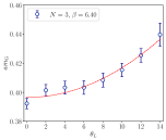
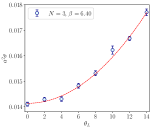
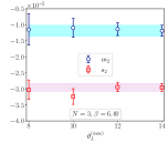
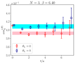
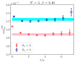
Figure 1: Results for $N=3$ with $\beta=6.40$ (finest lattice spacing explored).

We determined the mass gap of the theory (i.e., the mass of the lightest glueball state) and the string tension in lattice units for several values of $\beta$ and $\theta_{{\scriptscriptstyle{\mathrm{L}}}}$. The $\theta$ dependence was parameterized by Taylor expanding in up to the next-to-leading order, around $\theta=0$,

$$am_{{\scriptscriptstyle{\mathrm{G}}}}(\theta) = am_{{\scriptscriptstyle{0^{++}}}}\left[1+m_{2}\theta^{2}+\mathcal{O}(\theta^{2})\right],$$ (11)

$$a^{2}\sigma(\theta) = a^{2}\sigma\left[1+s_{2}\theta^{2}+\mathcal{O}(\theta^{2})\right]~{},$$ (12)

where the well-established fact that at $\theta=0$ the mass of the $0^{++}$ glueball is the lightest one in pure-Yang–Mills theories [99, 103, 104, 106]) was used. Using analyticity, and the renormalization property of the lattice imaginary-$\theta$ parameter, one simply has:

$$am_{{\scriptscriptstyle{\mathrm{G}}}}(\theta_{{\scriptscriptstyle{\mathrm{L}}}}) = am_{{\scriptscriptstyle{0^{++}}}}\left[1-m_{2}Z_{{}_{Q}}^{2}\theta_{\scriptscriptstyle{\mathrm{L}}}^{2}+\mathcal{O}(\theta_{\scriptscriptstyle{\mathrm{L}}}^{2})\right],$$ (13)

$$a^{2}\sigma(\theta_{{\scriptscriptstyle{\mathrm{L}}}}) = a^{2}\sigma\left[1-s_{2}Z_{{}_{Q}}^{2}\theta_{\scriptscriptstyle{\mathrm{L}}}^{2}+\mathcal{O}(\theta_{\scriptscriptstyle{\mathrm{L}}}^{2})\right].$$ (14)

We thus performed a best fit of our determinations of $m_{{\scriptscriptstyle{\mathrm{G}}}}(\theta_{{\scriptscriptstyle{\mathrm{L}}}})$ and $\sigma(\theta_{{\scriptscriptstyle{\mathrm{L}}}})$ as a function of $\theta_{\scriptscriptstyle{\mathrm{L}}}$ at fixed $\beta$ and determined the quantities $m_{2}Z_{{}_{Q}}^{2}$ and $s_{2}Z_{{}_{Q}}^{2}$. Since the value of $Z_{{}_{Q}}(\beta)$ was known for each $\beta$, we could obtain $m_{2}$ and $s_{2}$. Our results for $m_{2}$ and $s_{2}$ at $N=3$ are displayed in Fig. 1. They are very stable as a function of the fitting range, signaling that we are insensitive to the effects of higher-order corrections. We also display a few examples of plateaux of effective masses.

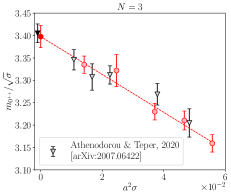
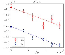
Figure 2: Continuum limit of our $N=3$ results for $m_{2}$ and $s_{2}$. We also computed the continuum limit of $m_{{\scriptscriptstyle{0^{++}}}}/\sqrt{\sigma}$, which is in perfect agreement with the previous result of [103].

In Fig. 2 we display the continuum extrapolation of our results for $m_{2}$ and $s_{2}$. We also extrapolated towards the continuum limit the dimensionless ratio $m_{{\scriptscriptstyle{0^{++}}}}/\sqrt{\sigma}$ in order to verify that our result is in agreement with the previous determination provided in Ref. [103].

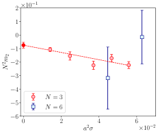
Figure 3: Continuum scaling of $N^{2}m_{2}$ and $N^{2}s_{2}$ for $N=3$ and $N=6$.

These are our final determinations for $N=3$, in the continuum limit,

$$\frac{m_{{\scriptscriptstyle{0^{++}}}}}{\sqrt{\sigma}}=3.398(25),\qquad\text{(continuum limit, $N=3$)},$$ (15)

$$m_{2}=-0.0083(23),\qquad\text{(continuum limit, $N=3$)},$$ (16)

$$s_{2}=-0.0258(14),\qquad\text{(continuum limit, $N=3$)}.$$ (17)

Concerning $N=6$, we obtained results only for two fairly fine lattice spacings, thus we cannot perform a continuum limit of these data alone. However, our data allowed for a first quantitative check of the following expected large-$N$ scaling:

$$m_{2}=\frac{\overline{m}_{2}}{N^{2}}+\mathcal{O}\left(\frac{1}{N^{4}}\right),\quad s_{2}=\frac{\overline{s}_{2}}{N^{2}}+\mathcal{O}\left(\frac{1}{N^{4}}\right).$$ (18)

Our $N=3$ and 6 results are perfectly compatible with this expected scaling, see Fig. 3. Thus, in the end we can quote the following estimates:

$$\overline{s}_{2}\simeq-0.23(1)\ ,\quad\overline{m}_{2}\simeq-0.075(20)\ .$$ (19)

4 Conclusions

The present manuscript reports on the main finding of [58]. We have studied the $\theta$-dependence of the $\mathrm{SU}(N)$ spectrum, focusing on the mass gap of the theory and on the string tension for $N=3$ and $N=6$.

For $\mathrm{SU}(3)$, in the continuum limit we found:

$$\frac{m_{{\scriptscriptstyle{\mathrm{G}}}}}{\sqrt{\sigma}}\Bigg{|}_{\theta=0}=\frac{m_{{\scriptscriptstyle{0^{++}}}}}{\sqrt{\sigma}}=3.398(25)~{},\quad m_{2}=-0.0083(23),\quad s_{2}=-0.0258(14),$$ (20)

where

$$m_{2}\equiv\frac{1}{2m_{{\scriptscriptstyle{0^{++}}}}}\times\frac{\mathrm{d}m_{{\scriptscriptstyle{\mathrm{G}}}}(\theta)}{\mathrm{d}\theta^{2}}\Bigg{|}_{\theta\,=\,0},\quad s_{2}\equiv\frac{1}{2\sigma}\times\frac{\mathrm{d}\sigma(\theta)}{\mathrm{d}\theta^{2}}\Bigg{|}_{\theta\,=\,0}.$$ (21)

The results obtained at $N=6$ also enabled us to check that the expected large-$N$ scaling was realized and to estimate:

$$m_{2}(N)\simeq\frac{-0.075(20)}{N^{2}}+\mathcal{O}\left(\frac{1}{N^{4}}\right),\quad s_{2}(N)\simeq\frac{-0.23(1)}{N^{2}}+\mathcal{O}\left(\frac{1}{N^{4}}\right).$$ (22)

Note that for $N=3$, the value of $m_{2}$ is very close to $s_{2}/2$. As a result, the coefficient $g_{2}$ of the order $\mathcal{O}(\theta^{2})$ correction to the dimensionless ratio $m_{\scriptscriptstyle{\mathrm{G}}}/\sqrt{\sigma}$,

$$\left(\frac{m_{\scriptscriptstyle{\mathrm{G}}}}{\sqrt{\sigma}}\right)(\theta)=\frac{m_{\scriptscriptstyle{0^{++}}}}{\sqrt{\sigma}}\left(1+g_{2}\theta^{2}+\mathcal{O}(\theta^{4})\right),$$ (23)

is compatible with zero within two standard deviations,

$$g_{2}=m_{2}-\frac{s_{2}}{2}=0.0046(24)~{}.$$ (24)

We are not aware of any general theoretical argument that would dictate the $\theta$-independence of this dimensionless ratio. Actually, we can provide a counter-example to this. In Refs. [64, 65, 67], the $\theta$-dependence of the $\mathrm{SU}(N)$ deconfinement critical temperature $T_{c}$ was investigated for $N\geq 3$ (for a first SU(2) study see [107]). It was concluded that if

$$T_{c}(\theta)=T_{c}[1-R\theta^{2}+\mathcal{O}(\theta^{4})]~{},$$ (25)

then

$$R(N=3)=0.0178(5)~{},\quad R(N)=\frac{0.159(4)}{N^{2}}+\mathcal{O}\left(\frac{1}{N^{4}}\right)\quad(N>3)~{}.$$ (26)

Using our result for $s_{2}$, we would then find,

$$\frac{T_{c}(\theta)}{\sqrt{\sigma(\theta)}}=\frac{T_{c}}{\sqrt{\sigma}}[1-t_{2}\theta^{2}+\mathcal{O}(\theta^{4})]~{},$$ (27)

and the coefficient $t_{2}$ would then be non-vanishing,

$$t_{2}=R+\frac{s_{2}}{2}=0.0049(9)~{}.$$ (28)

It is interesting to observe that the $\theta$-dependence of $m_{{\scriptscriptstyle{\mathrm{G}}}}$ and $\sigma$ in large-$N$ Yang–Mills theories has been also addressed within holographic models in [108], providing the following prediction:

$$\frac{s_{2}}{m_{2}}=\frac{\overline{s}_{2}}{\overline{m}_{2}}=4,\qquad\qquad\text{(holography),}$$ (29)

which nicely agrees with our lattice result

$$\frac{s_{2}}{m_{2}}=\frac{\overline{s}_{2}}{\overline{m}_{2}}=3.07(82),\qquad\qquad\text{(lattice).}$$ (30)

On the other hand, Ref. [108] predicts that the ratio $T_{c}(\theta)/m_{{\scriptscriptstyle{\mathrm{G}}}}(\theta)$ is $\theta$-independent at $\mathcal{O}(\theta^{2})$, i.e., $R/m_{2}=-1$, in contrast with our lattice result $R/m_{2}=-2.14(57)$ indicating that $T_{c}(\theta)/m_{{\scriptscriptstyle{\mathrm{G}}}}(\theta)$ has a non-trivial $\theta$-dependence already at leading order in $\theta$.

Finally, we recall the interesting role played by $m_{2}$, identified in [109, 110] in the estimation of the systematic error introduced in lattice spectra calculations performed at fixed topological sector. At a fixed value $Q$ of the topological charge, the following approximate relation holds for the mass $M$ of any bound state,

$$\frac{M^{(Q)}-M}{M}\approx\frac{M_{2}}{2\chi V}~{},$$ (31)

where $\chi=\braket{Q^{2}}/V$ is the topological susceptibility and $M_{2}$ is the order $\mathcal{O}(\theta)^{2}$ coefficient of $M(\theta)=M[1+M_{2}\theta^{2}+\mathcal{O}(\theta^{4})]$. For $N=3$ the topological susceptibility is roughly $\chi\simeq(1\text{ fm})^{-4}$. For a standard lattice volume of $V=(1.5\text{ fm})^{4}$, one has the following bound on the systematic error on the numerical estimation of the lightest $0^{++}$ glueball:

$$\frac{\Delta m_{{\scriptscriptstyle{0^{++}}}}}{m_{{\scriptscriptstyle{0^{++}}}}}\Bigg{|}_{N=3}\approx\frac{m_{2}}{2\chi V}\approx-0.08\%.$$ (32)

This bound will become even more favorable at larger value of $N$, since $\chi$ does not change appreciably with $N$, while $m_{2}\sim\mathcal{O}(1/N^{2})$.

References

- [1] E. Witten, Current Algebra Theorems for the Goldstone Boson, Nucl. Phys. B 156 (1979) 269.
- [2] G. Veneziano, Without Instantons, Nucl. Phys. B 159 (1979) 213.
- [3] K. Kawarabayashi and N. Ohta, The Problem of in the Large Limit: Effective Lagrangian Approach, Nucl. Phys. B 175 (1980) 477.
- [4] E. Witten, Large Chiral Dynamics, Annals Phys. 128 (1980) 363.
- [5] S. Coleman, Aspects of Symmetry: Selected Erice Lectures. Cambridge University Press, Cambridge, U.K., 1985.
- [6] D. J. Gross, R. D. Pisarski and L. G. Yaffe, QCD and Instantons at Finite Temperature, Rev. Mod. Phys. 53 (1981) 43.
- [7] T. Schäfer and E. V. Shuryak, Instantons in QCD, Rev. Mod. Phys. 70 (1998) 323 [hep-ph/9610451].
- [8] A. D’Adda, M. Lüscher and P. Di Vecchia, A Expandable Series of Nonlinear Sigma Models with Instantons, Nucl. Phys. B 146 (1978) 63.
- [9] E. Witten, Instantons, the Quark Model, and the Expansion, Nucl. Phys. B 149 (1979) 285.
- [10] T. G. Kovacs, E. T. Tomboulis and Z. Schram, Topology on the lattice: 2-d Yang-Mills theories with a theta term, Nucl. Phys. B 454 (1995) 45 [hep-th/9505005].
- [11] C. Bonati and P. Rossi, Topological susceptibility of two-dimensional gauge theories, Phys. Rev. D 99 (2019) 054503 [1901.09830].
- [12] C. Bonati and P. Rossi, Topological effects in continuum two-dimensional gauge theories, Phys. Rev. D 100 (2019) 054502 [1908.07476].
- [13] R. Jackiw, Introduction to the Yang-Mills Quantum Theory, Rev. Mod. Phys. 52 (1980) 661.
- [14] D. Gaiotto, A. Kapustin, Z. Komargodski and N. Seiberg, Theta, Time Reversal, and Temperature, JHEP 05 (2017) 091 [1703.00501].
- [15] C. Bonati and M. D’Elia, Topological critical slowing down: variations on a toy model, Phys. Rev. E 98 (2018) 013308 [1709.10034].
- [16] P. Di Vecchia and G. Veneziano, Chiral Dynamics in the Large Limit, Nucl. Phys. B 171 (1980) 253.
- [17] G. Grilli di Cortona, E. Hardy, J. Pardo Vega and G. Villadoro, The QCD axion, precisely, JHEP 01 (2016) 034 [1511.02867].
- [18] F.-K. Guo and U.-G. Meißner, Cumulants of the QCD topological charge distribution, Phys. Lett. B 749 (2015) 278 [1506.05487].
- [19] Z.-Y. Lu, M.-L. Du, F.-K. Guo, U.-G. Meißner and T. Vonk, QCD -vacuum energy and axion properties, JHEP 05 (2020) 001 [2003.01625].
- [20] N. R. Acharya, F.-K. Guo, M. Mai and U.-G. Meißner, -dependence of the lightest meson resonances in QCD, Phys. Rev. D 92 (2015) 054023 [1507.08570].
- [21] A. Boccaletti and D. Nogradi, The semi-classical approximation at high temperature revisited, JHEP 03 (2020) 045 [2001.03383].
- [22] C. Bonati, M. D’Elia, M. Mariti, G. Martinelli, M. Mesiti, F. Negro et al., Axion phenomenology and -dependence from lattice QCD, JHEP 03 (2016) 155 [1512.06746].
- [23] P. Petreczky, H.-P. Schadler and S. Sharma, The topological susceptibility in finite temperature QCD and axion cosmology, Phys. Lett. B 762 (2016) 498 [1606.03145].
- [24] J. Frison, R. Kitano, H. Matsufuru, S. Mori and N. Yamada, Topological susceptibility at high temperature on the lattice, JHEP 09 (2016) 021 [1606.07175].
- [25] S. Borsanyi et al., Calculation of the axion mass based on high-temperature lattice quantum chromodynamics, Nature 539 (2016) 69 [1606.07494].
- [26] C. Bonati, M. D’Elia, G. Martinelli, F. Negro, F. Sanfilippo and A. Todaro, Topology in full QCD at high temperature: a multicanonical approach, JHEP 11 (2018) 170 [1807.07954].
- [27] F. Burger, E.-M. Ilgenfritz, M. P. Lombardo and A. Trunin, Chiral observables and topology in hot QCD with two families of quarks, Phys. Rev. D 98 (2018) 094501 [1805.06001].
- [28] TWQCD collaboration, Y.-C. Chen, T.-W. Chiu and T.-H. Hsieh, Topological susceptibility in finite temperature QCD with physical (u/d,s,c) domain-wall quarks, Phys. Rev. D 106 (2022) 074501 [2204.01556].
- [29] A. Athenodorou, C. Bonanno, C. Bonati, G. Clemente, F. D’Angelo, M. D’Elia et al., Topological susceptibility of Nf = 2 + 1 QCD from staggered fermions spectral projectors at high temperatures, JHEP 10 (2022) 197 [2208.08921].
- [30] B. Alles, M. D’Elia and A. Di Giacomo, Topological susceptibility at zero and finite T in SU(3) Yang-Mills theory, Nucl. Phys. B 494 (1997) 281 [hep-lat/9605013].
- [31] B. Alles, M. D’Elia and A. Di Giacomo, Topology at zero and finite in Yang–Mills theory, Phys. Lett. B 412 (1997) 119 [hep-lat/9706016].
- [32] L. Del Debbio, L. Giusti and C. Pica, Topological susceptibility in the gauge theory, Phys. Rev. Lett. 94 (2005) 032003 [hep-th/0407052].
- [33] L. Del Debbio, H. Panagopoulos and E. Vicari, dependence of gauge theories, JHEP 08 (2002) 044 [hep-th/0204125].
- [34] M. D’Elia, Field theoretical approach to the study of theta dependence in Yang-Mills theories on the lattice, Nucl. Phys. B 661 (2003) 139 [hep-lat/0302007].
- [35] B. Lucini, M. Teper and U. Wenger, Topology of gauge theories at and , Nucl. Phys. B 715 (2005) 461 [hep-lat/0401028].
- [36] L. Giusti, S. Petrarca and B. Taglienti, dependence of the vacuum energy in the gauge theory from the lattice, Phys. Rev. D 76 (2007) 094510 [0705.2352].
- [37] E. Vicari and H. Panagopoulos, dependence of gauge theories in the presence of a topological term, Phys. Rept. 470 (2009) 93 [0803.1593].
- [38] H. Panagopoulos and E. Vicari, The gauge theory with an imaginary term, JHEP 11 (2011) 119 [1109.6815].
- [39] C. Bonati, M. D’Elia, H. Panagopoulos and E. Vicari, Change of Dependence in Gauge Theories Across the Deconfinement Transition, Phys. Rev. Lett. 110 (2013) 252003 [1301.7640].
- [40] M. Cè, C. Consonni, G. P. Engel and L. Giusti, Non-Gaussianities in the topological charge distribution of the Yang–Mills theory, Phys. Rev. D 92 (2015) 074502 [1506.06052].
- [41] M. Cè, M. Garcia Vera, L. Giusti and S. Schaefer, The topological susceptibility in the large- limit of SU() Yang-Mills theory, Phys. Lett. B 762 (2016) 232 [1607.05939].
- [42] E. Berkowitz, M. I. Buchoff and E. Rinaldi, Lattice QCD input for axion cosmology, Phys. Rev. D 92 (2015) 034507 [1505.07455].
- [43] S. Borsanyi, M. Dierigl, Z. Fodor, S. Katz, S. Mages, D. Nogradi et al., Axion cosmology, lattice QCD and the dilute instanton gas, Phys. Lett. B 752 (2016) 175 [1508.06917].
- [44] C. Bonati, M. D’Elia and A. Scapellato, dependence in Yang-Mills theory from analytic continuation, Phys. Rev. D 93 (2016) 025028 [1512.01544].
- [45] C. Bonati, M. D’Elia, P. Rossi and E. Vicari, dependence of 4D gauge theories in the large- limit, Phys. Rev. D 94 (2016) 085017 [1607.06360].
- [46] C. Bonati, M. Cardinali and M. D’Elia, dependence in trace deformed Yang-Mills theory: a lattice study, Phys. Rev. D 98 (2018) 054508 [1807.06558].
- [47] C. Bonati, M. Cardinali, M. D’Elia and F. Mazziotti, -dependence and center symmetry in Yang-Mills theories, Phys. Rev. D 101 (2020) 034508 [1912.02662].
- [48] M. Campostrini and P. Rossi, expansion of the topological susceptibility in the models, Phys. Lett. B 272 (1991) 305.
- [49] L. Del Debbio, G. M. Manca, H. Panagopoulos, A. Skouroupathis and E. Vicari, -dependence of the spectrum of gauge theories, JHEP 06 (2006) 005 [hep-th/0603041].
- [50] P. Rossi, Effective Lagrangian of models in the large limit, Phys. Rev. D D94 (2016) 045013 [1606.07252].
- [51] E. Vicari, Monte Carlo simulation of lattice models at large , Phys. Lett. B 309 (1993) 139 [hep-lat/9209025].
- [52] C. Bonanno, C. Bonati and M. D’Elia, Topological properties of models in the large- limit, JHEP 01 (2019) 003 [1807.11357].
- [53] M. Berni, C. Bonanno and M. D’Elia, Large- expansion and -dependence of models beyond the leading order, Phys. Rev. D 100 (2019) 114509 [1911.03384].
- [54] M. Berni, C. Bonanno and M. D’Elia, -dependence in the small- limit of models, Phys. Rev. D 102 (2020) 114519 [2009.14056].
- [55] C. Bonanno, M. D’Elia and F. Margari, Topological susceptibility of the 2D CP1 or O(3) nonlinear model: Is it divergent or not?, Phys. Rev. D 107 (2023) 014515 [2208.00185].
- [56] D. Nogradi, An ideal toy model for confining, walking and conformal gauge theories: the O(3) sigma model with theta-term, JHEP 05 (2012) 089 [1202.4616].
- [57] B. Alles, M. Giordano and A. Papa, Behavior near of the mass gap in the two-dimensional O(3) non-linear sigma model, Phys. Rev. B 90 (2014) 184421 [1409.1704].
- [58] C. Bonanno, C. Bonati, M. Papace and D. Vadacchino, The -dependence of the Yang-Mills spectrum from analytic continuation, JHEP 05 (2024) 163 [2402.03096].
- [59] G. Bhanot and F. David, The Phases of the Model for Imaginary , Nucl. Phys. B 251 (1985) 127.
- [60] V. Azcoiti, G. Di Carlo, A. Galante and V. Laliena, New proposal for numerical simulations of theta vacuum - like systems, Phys. Rev. Lett. 89 (2002) 141601 [hep-lat/0203017].
- [61] B. Alles and A. Papa, Mass gap in the non-linear sigma model with a term, Phys. Rev. D 77 (2008) 056008 [0711.1496].
- [62] M. Imachi, M. Kambayashi, Y. Shinno and H. Yoneyama, The -term, model and the inversion approach in the imaginary- method, Prog. Theor. Phys. 116 (2006) 181.
- [63] S. Aoki, R. Horsley, T. Izubuchi, Y. Nakamura, D. Pleiter, P. E. L. Rakow et al., The Electric dipole moment of the nucleon from simulations at imaginary vacuum angle theta, 0808.1428.
- [64] M. D’Elia and F. Negro, dependence of the deconfinement temperature in Yang–Mills theories, Phys. Rev. Lett. 109 (2012) 072001 [1205.0538].
- [65] M. D’Elia and F. Negro, Phase diagram of Yang-Mills theories in the presence of a term, Phys. Rev. D 88 (2013) 034503 [1306.2919].
- [66] C. Bonanno, C. Bonati and M. D’Elia, Large- Yang-Mills theories with milder topological freezing, JHEP 03 (2021) 111 [2012.14000].
- [67] C. Bonanno, M. D’Elia and L. Verzichelli, The -dependence of the critical temperature at large , JHEP 02 (2024) 156 [2312.12202].
- [68] M. Campostrini, A. Di Giacomo and H. Panagopoulos, The Topological Susceptibility on the Lattice, Phys. Lett. B 212 (1988) 206.
- [69] B. Berg, Dislocations and Topological Background in the Lattice Model, Phys. Lett. B 104 (1981) 475.
- [70] Y. Iwasaki and T. Yoshie, Instantons and Topological Charge in Lattice Gauge Theory, Phys. Lett. B 131 (1983) 159.
- [71] S. Itoh, Y. Iwasaki and T. Yoshie, Stability of Instantons on the Lattice and the Renormalized Trajectory, Phys. Lett. B 147 (1984) 141.
- [72] M. Teper, Instantons in the Quantized Vacuum: A Lattice Monte Carlo Investigation, Phys. Lett. B 162 (1985) 357.
- [73] E.-M. Ilgenfritz, M. Laursen, G. Schierholz, M. Müller-Preussker and H. Schiller, First Evidence for the Existence of Instantons in the Quantized Lattice Vacuum, Nucl. Phys. B 268 (1986) 693.
- [74] M. Campostrini, A. Di Giacomo, H. Panagopoulos and E. Vicari, Topological Charge, Renormalization and Cooling on the Lattice, Nucl. Phys. B 329 (1990) 683.
- [75] B. Alles, L. Cosmai, M. D’Elia and A. Papa, Topology in models on the lattice: A Critical comparison of different cooling techniques, Phys. Rev. D 62 (2000) 094507 [hep-lat/0001027].
- [76] APE collaboration, M. Albanese et al., Glueball Masses and String Tension in Lattice QCD, Phys. Lett. B 192 (1987) 163.
- [77] C. Morningstar and M. J. Peardon, Analytic smearing of SU(3) link variables in lattice QCD, Phys. Rev. D 69 (2004) 054501 [hep-lat/0311018].
- [78] M. Lüscher, Trivializing maps, the Wilson flow and the HMC algorithm, Commun. Math. Phys. 293 (2010) 899 [0907.5491].
- [79] M. Lüscher, Properties and uses of the Wilson flow in lattice QCD, JHEP 08 (2010) 071 [1006.4518].
- [80] M. Luscher and P. Weisz, Perturbative analysis of the gradient flow in non-abelian gauge theories, JHEP 02 (2011) 051 [1101.0963].
- [81] C. Bonati and M. D’Elia, Comparison of the gradient flow with cooling in pure gauge theory, Phys. Rev. D D89 (2014) 105005 [1401.2441].
- [82] C. Alexandrou, A. Athenodorou and K. Jansen, Topological charge using cooling and the gradient flow, Phys. Rev. D 92 (2015) 125014 [1509.04259].
- [83] M. Creutz, Overrelaxation and Monte Carlo Simulation, Phys. Rev. D 36 (1987) 515.
- [84] M. Creutz, Monte Carlo Study of Quantized Gauge Theory, Phys. Rev. D 21 (1980) 2308.
- [85] A. D. Kennedy and B. J. Pendleton, Improved Heat Bath Method for Monte Carlo Calculations in Lattice Gauge Theories, Phys. Lett. B 156 (1985) 393.
- [86] M. Hasenbusch, Fighting topological freezing in the two-dimensional model, Phys. Rev. D 96 (2017) 054504 [1706.04443].
- [87] B. Alles, G. Boyd, M. D’Elia, A. Di Giacomo and E. Vicari, Hybrid Monte Carlo and topological modes of full QCD, Phys. Lett. B 389 (1996) 107 [hep-lat/9607049].
- [88] L. Del Debbio, G. M. Manca and E. Vicari, Critical slowing down of topological modes, Phys. Lett. B 594 (2004) 315 [hep-lat/0403001].
- [89] ALPHA collaboration, S. Schaefer, R. Sommer and F. Virotta, Critical slowing down and error analysis in lattice QCD simulations, Nucl. Phys. B 845 (2011) 93 [1009.5228].
- [90] C. Bonanno, Lattice determination of the topological susceptibility slope of CPN-1 models at large , Phys. Rev. D 107 (2023) 014514 [2212.02330].
- [91] C. Bonanno, G. Clemente, M. D’Elia, L. Maio and L. Parente, Full QCD with milder topological freezing, JHEP 08 (2024) 236 [2404.14151].
- [92] C. Bonanno, M. D’Elia, B. Lucini and D. Vadacchino, Towards glueball masses of large-N SU(N) pure-gauge theories without topological freezing, Phys. Lett. B 833 (2022) 137281 [2205.06190].
- [93] J. L. Dasilva Golán, C. Bonanno, M. D’Elia, M. García Pérez and A. Giorgieri, The twisted gradient flow strong coupling with parallel tempering on boundary conditions, PoS LATTICE2023 (2024) 354 [2312.09212].
- [94] C. Bonanno, J. L. Dasilva Golán, M. D’Elia, M. García Pérez and A. Giorgieri, The twisted gradient flow strong coupling without topological freezing, Eur. Phys. J. C 84 (2024) 916 [2403.13607].
- [95] B. Berg and A. Billoire, Glueball spectroscopy in su() lattice gauge theory (i), Nuclear Physics B 221 (1983) 109.
- [96] M. Teper, An improved method for lattice glueball calculations, Physics Letters B 183 (1987) 345.
- [97] M. J. Teper, SU() gauge theories in -dimensions, Phys. Rev. D 59 (1999) 014512 [hep-lat/9804008].
- [98] B. Lucini and M. Teper, gauge theories in four-dimensions: Exploring the approach to , JHEP 06 (2001) 050 [hep-lat/0103027].
- [99] B. Lucini, M. Teper and U. Wenger, Glueballs and -strings in gauge theories: Calculations with improved operators, JHEP 06 (2004) 012 [hep-lat/0404008].
- [100] B. Blossier, M. Della Morte, G. von Hippel, T. Mendes and R. Sommer, On the generalized eigenvalue method for energies and matrix elements in lattice field theory, JHEP 04 (2009) 094 [0902.1265].
- [101] B. Lucini, A. Rago and E. Rinaldi, Glueball masses in the large- limit, JHEP 08 (2010) 119 [1007.3879].
- [102] E. Bennett, J. Holligan, D. K. Hong, J.-W. Lee, C. J. D. Lin, B. Lucini et al., Glueballs and strings in Yang-Mills theories, Phys. Rev. D 103 (2021) 054509 [2010.15781].
- [103] A. Athenodorou and M. Teper, The glueball spectrum of SU(3) gauge theory in 3 + 1 dimensions, JHEP 11 (2020) 172 [2007.06422].
- [104] A. Athenodorou and M. Teper, SU(N) gauge theories in 3+1 dimensions: glueball spectrum, string tensions and topology, JHEP 12 (2021) 082 [2106.00364].
- [105] P. de Forcrand, G. Schierholz, H. Schneider and M. Teper, The String and Its Tension in SU(3) Lattice Gauge Theory: Towards Definitive Results, Phys. Lett. B 160 (1985) 137.
- [106] D. Vadacchino, A review on Glueball hunting, 2305.04869.
- [107] N. Yamada, M. Yamazaki and R. Kitano, dependence of in SU(2) Yang-Mills theory, 2411.00375.
- [108] F. Bigazzi, A. L. Cotrone and R. Sisca, Notes on Dependence in Holographic Yang–Mills, JHEP 08 (2015) 090 [1506.03826].
- [109] R. Brower, S. Chandrasekharan, J. W. Negele and U. J. Wiese, QCD at fixed topology, Phys. Lett. B 560 (2003) 64 [hep-lat/0302005].
- [110] S. Aoki, H. Fukaya, S. Hashimoto and T. Onogi, Finite volume QCD at fixed topological charge, Phys. Rev. D 76 (2007) 054508 [0707.0396].