Dissecting Buchdahl’s limit: A surgeon’s guide to compact objects

Abstract

One of the theoretical motivations behind the belief that black holes as described by general relativity exist in nature is that it is hard to find matter configurations that mimic their properties, especially their compactness. One of the classic results that goes in this direction is the so-called Buchdahl limit: a bound for the maximum compactness that, under a few assumptions, static fluid spheres in hydrostatic equilibrium can possibly have. We highlight two of the main assumptions that could be violated in physically realistic situations: i) isotropy and ii) an outward-decreasing monotonicity of the density profile, which, as we discuss in detail, can be understood as a form of energy condition. We construct a pair of toy models that exemplify how the Buchdahl limit can be overcome if any of these two assumptions is individually relaxed. In particular, we show that relaxing the monotonicity assumption alone yields a new, less restrictive compactness limit as long as the energy density is not allowed to become negative. If negative energies are permitted, the compactness of these toy models can be as close to the black hole limit as desired. We also discuss how these toy models represent some of the main features of realistic systems, and how they could be extended to find more refined models.

I Introduction

Verifying whether the dark and compact objects that we observe in the universe strictly correspond to general relativistic black holes is still an open question that is attracting a large amount of interest and effort Collmar et al. (1998); Abramowicz et al. (2002); Carballo-Rubio et al. (2022). In an astrophysical context, any object that displays a sufficiently large gravitational mass in a sufficiently small region is believed to be a black hole. Probing and analyzing astrophysical black-hole systems could be our best chance to find a robust path beyond standard general relativity.

On theoretical grounds, the first result pointing out that black holes might be inevitable can be traced back to Chandrasekhar’s mass limit for white dwarf stars Chandrasekhar (1931, 1931). As a dwarf star increases its mass, the electrons become more relativistic, and a mass limit appears at which the pressure provided by Pauli’s exclusion principle for fermions is unable to counteract gravity. An equivalent limit appears for neutron stars, now with the exclusion applied to neutrons Oppenheimer and Volkoff (1939). In both cases, adding some more mass to the limiting configuration would cause the star to collapse into a black hole. It is interesting to recall that these limits are found even without invoking pure general relativistic effects.

Making use of the full Einstein equations one can find, in addition to the previous limits, some bounds to the compactness of those stars Nilsson and Uggla (2000). We shall define the compactness $C(R)$ of a spherically symmetric configuration to be the quotient between twice the total mass of the object $2M$ and its radius $R$: $C(R)=2M/R$. For example, typical neutron stars have compactness of around $C(R)\sim 0.4$. This is to be contrasted with the maximum compactness attainable in general relativity: the limit $C(R)=1$ representing a black hole, i.e. a completely collapsed star.

Now, armed with the full Einstein equations one can analyze whether there could be, at least in principle, stellar objects more compact than neutron stars. Here comes the surprise. Under mild conditions there exists a limit to the maximum compactness attainable by a static, spherically symmetric sphere of perfect fluid matching the Schwarzschild metric at its surface. This so-called Buchdahl limit Buchdahl (1959); Bondi (1964); Wald (1984) is $C(R)<8/9$, and its origins can be traced back to Schwarzschild’s work on stellar interiors Schwarzschild (1916). Buchdahl proved that $C(R)<8/9$ as a theorem, making no strong hypothesis regarding the equation of state of matter beyond being barotropic. Its two central assumptions are just the isotropy of the fluid, namely that pressures in the tangential and radial directions are equal, and that the energy density is a positive, (outwards) monotonically decreasing function of the radius.

Our aim in this paper is to explore the consequences and the physical viability of relaxing each individual assumption behind the Buchdahl theorem (assuming for simplicity a Schwarzschild exterior, i.e., vacuum, staticity and spherical symmetry). In particular, we are interested in understanding whether such relaxation leads to new, less restrictive, compactness bounds, or to no further compactness bounds at all. We restrict ourselves to static and spherically symmetric configurations, since potential generalizations to stationary and axisymmetric scenarios are far from straightforward.

First, we will explore the role of the monotonicity and positivity of the energy density by introducing a stellar model composed of two thick layers of constant energy density: an internal core and an external crust, with the condition that the density is always larger for the crust than for the core. For this model, we analyze two very different situations: one in which we constrain the core density to be positive, and another in which we allow it to take negative values. We show that, in the first situation, a new bound on the compactness arises. We find numerically that this bound is approximately $C(R)\leq 0.9706$ (which is less restrictive than the Buchdahl bound $C(R)<8/9\simeq 0.888$, but still well-below the black hole compactness $C(R)=1$). Furthermore, we conjecture that a general bound on the compactness exists for a generic positive density independently of its behaviour, but at this stage we are unable to provide a complete proof. Meanwhile, when we allow for negative densities in the core, we show that there is no compactness bound; hence it is possible to build solutions as close to the black hole limit as desired, at least as long as we do not impose any energy condition on the fluid.

Within these bilayered models we find one specially simple and interesting: a stellar structure that we have decided to call anti-de Sitter star. It is similar to a gravastar Mazur and Mottola (2023) but with an anti-de Sitter (AdS) core instead of a de Sitter core. These stars have also some similarities with AdS black shells Danielsson et al. (2017), the central difference being precisely their compactness. While AdS black shells have compactness around the Buchdahl limit, AdS stars have compactness close to the black hole limit. As we will discuss, it is interesting to highlight that these AdS stars appear as idealizations of the semiclassical stellar configurations found in Arrechea et al. (2021, 2024).

Secondly, as a separate situation, we will test the relevance of relaxing the isotropy of the pressure. For this, we present a toy model consisting of a thin shell matching an internal Minkowskian core with an external Schwarzschild solution. We show that the shell can be placed as close to its Schwarzschild radius as desired, making the configuration arbitrarily close to the black hole compactness. However, the price to pay is that the distributional tangential pressures of the shell grow without upper bounds as this limit is approached, while the surface density remains finite. In that sense, the Dominant Energy Condition (DEC) is guaranteed to be violated beyond some compactness. In other words, imposing energy conditions sets a compactness bound in the anisotropic case. We revisit and compare our findings with similar results in the literature presenting bounds for anisotropic configurations.

In a final section we also provide a detailed discussion on how these toy models capture some of the main physical ingredients that are required to violate the Buchdahl limit, and propose ways in which more realistic models can be built taking these toy models as departure points. We also analyze some of the arguments that are sometimes used to discard the possibility that these objects are physically meaningful, e.g., the putative violations of causality that might arise if the DEC is violated.

The paper is structured as follows. In Section II, we revisit Buchdahl’s theorem as a warm-up exercise to show how the isotropy of the pressures and monotonicity of the positive density function enter into the proof. In Section III, we discuss the toy model that illustrates how to violate the Buchdahl limit relaxing the monotonicity of the density. In Subsec. III.1, we restrict ourselves to positive densities and show that there is an upper limit to the compactness that these objects can display, which is maximized when the internal core is “empty” (i.e., vanishing density in the internal layer). We conjecture that for positive monotonically increasing densities there should always exist an upper bound to the compactness. In Subsec. III.3, we consider the possibility of a negative inner core density, and we show that there is no limit to the compactness that these objects can have, illustrating the fact that allowing for any kind of negative density inner core would open the possibility of having objects as close to the black hole’s compactness as desired. In Section IV, we discuss the AdS star model: a particular case of bilayered star in which the inner core is described by AdS spacetime and the outer layer is reduced to a thin shell. In Section V, we introduce the model of a shell matching an inner Minkowskian core with an outer Schwarzschild metric. We show that it can get arbitrarily close to the compactness of a black hole, although there is a threshold beyond which energy conditions are violated. We use this result to illustrate the possibility of violating Buchdahl’s limit by considering anisotropic pressures. Finally, we conclude in Section VI with a discussion on the features of potentially realistic configurations that are reproduced by these toy models, and ways in which they could be improved in the future. Appendix A discusses the constant density perfect fluid spheres, and Appendix B provides the details of the construction of the AdS stars and the second toy model, i.e., the shell matching the internal Minkowskian or AdS core with the external Schwarzschild metric.

Notation and conventions.

In this article, we use the signature $(-,+,+,+)$ for the spacetime metric, and we work in geometric units with $c=G=1$. Einstein’s summation convention is used throughout the work unless otherwise stated. For the connection and curvature tensors we use the conventions of Wald’s book Wald (1984), which we summarize here for completeness. The covariant derivative of a vector is given by $\nabla_{a}V^{b}=\partial_{a}V^{b}+\Gamma^{b}{}_{ac}V^{c}$; the commutator of covariant derivatives is $[\nabla_{a},\nabla_{b}]V^{c}=-R_{abd}{}^{c}V^{d}$ and, finally, the Ricci tensor is obtained as $R_{ab}:=R_{acb}{}^{c}$. The symbolic computations presented here were performed with the assistance of the software xAct Martin-Garcia et al. (2021).

II Buchdahl’s limit

We first review the Buchdahl limit in an attempt to present with clarity the steps in its derivation. The purpose of this section is twofold, serving both to settle the notation that will be used during this work, and to pose the problem that we will be studying. Importantly, we will enumerate the hypotheses behind the Buchdahl limit, i.e., the existence in general relativity of an upper bound to the compactness of stars in hydrostatic equilibrium.

Consider the following line element that represents static and spherically-symmetric spacetimes:

$$ds^{2}=-f(r)dt^{2}+h(r)dr^{2}+r^{2}d\Omega^{2}_{2}.$$ (1)

For some purposes it is useful to use an alternative set of functions:

$$f(r)=e^{2\Phi(r)},~{}~{}~{}~{}~{}~{}~{}~{}h(r)=\frac{1}{1-\frac{2m(r)}{r}},$$ (2)

where $\Phi(r)$ is the redshift function and $m(r)$ is the Misner-Sharp mass function Misner and Sharp (1964); Hernandez and Misner (1966).

We want to study solutions representing a star composed by the stress-energy tensor (SET) of a perfect fluid, i.e., a tensor that reads:

$$T_{ab}=\rho u_{a}u_{b}+p\left(g_{ab}+u_{a}u_{b}\right),$$ (3)

where $u^{a}$ is the vector field representing the velocity of the fluid, $\rho$ is the density of the fluid, and $p$ is the pressure. Staticity requires that the vector $u^{a}$ is aligned with the timelike Killing vector associated with the staticity of the spacetime, $u^{a}=e^{-\Phi}\delta^{a}_{\ t}$. Furthermore, we will restrict our considerations to barotropic fluids, i.e., fluids admitting an equation of state of the form $\rho=\rho(p)$. We focus on solutions that are empty, i.e., with $\rho,p=0$, for $r>R$, corresponding to a sphere filled with a perfect fluid that matches an exterior vacuum spherically symmetric static solution at $r=R$. In virtue of Birkhoff’s theorem, the only exterior solution fulfilling these properties is the Schwarzschild solution, and hence we have that for $r>R$:

$$\Phi(r)=\frac{1}{2}\log\left(1-\frac{2M}{r}\right),$$ (4)

$$m(r)=M,$$ (5)

with $M\in\mathbb{R}$.

If we plug the ansatz from Eqs. (1) and (2) into Einstein equations, we are led to the following equation that determines $\Phi(r)$:

$$\frac{d\Phi(r)}{dr}=\frac{m(r)+4\pi r^{3}p}{r\left[r-2m(r)\right]},$$ (6)

with $m(r)$ defined in terms of an integral of the energy density given in Eq. (3),

$$m(r)=4\pi\int dr^{\prime}r^{\prime 2}\rho(r^{\prime}).$$ (7)

Combining Eq. (6) with the conservation relation for the SET,

$$p^{\prime}(r)=-\left(\rho+p\right)\Phi^{\prime},$$ (8)

we arrive at the Tolman-Oppenheimer-Volkoff (TOV) equation, which is given by

$$\frac{dp}{dr}=-(p+\rho)\frac{m(r)+4\pi r^{3}p}{r\left[r-2m(r)\right]}.$$ (9)

Alternatively, this equation can be rewritten using a local compactness function defined in terms of the Misner-Sharp mass function as $C(r)=2m(r)/r$:

$$\frac{dp}{dr}=-\frac{(p+\rho)}{2r}~{}\frac{\left[C(r)+8\pi r^{2}p\right]}{\left[1-C(r)\right]}.$$ (10)

Expressions (7–9), together with the equation of state $\rho(p)$, form a closed system of differential equations to be solved for $\Phi,m,\rho$, and $p$. In order to find a specific solution, we take a central density $\rho(0)=\rho_{c}$ which, by virtue of the equation of state determines a central pressure $p(0)=p_{c}$. This allows to integrate the TOV equation together with the equation of state and Eq. (7) for $m(r)$. Finally, it is possible to determine the redshift by integrating Eq. (6) (or, equivalently, Eq. (8)) and matching the redshift of the surface $r=R$ with its Schwarzschild counterpart, given in Eq. (4).

Buchdahl’s limit sets an upper bound on the total mass $M$ that a star with a given radius $R$ can have. To understand what we need in order to surpass Buchdahl’s compactness limit, we will express its underlying assumptions in its most conservative version. This is best done by stating the result in the form of a theorem.

Buchdahl’s theorem: Consider the problem of finding the solution to the TOV equations (7–9) assuming a perfect fluid with an equation of state that fulfils the following properties:

1. The redshift function $f(r)$ is at least a $\mathcal{C}^{1}$ function while $h(r)$ at least $\mathcal{C}^{0}$. We integrate the equations from the centre $r=0$ with given pressures and densities $\{\rho_{c},p_{c}\}$ towards the surface $r=R$, defined by the condition $p(R)=0$. From that point on ($r>R$) we match an exterior (vacuum) Scwharzschild solution with $\rho=p=0$, independently of the value of $\rho\left(R^{-}\right)$.

2. The density is a monotonically decreasing function. The continuity and monotonicity assumptions along with the boundary conditions require that $\rho(r)\geq 0$.

For any such solution, the compactness satisfies the inequality $C(R)<8/9$.

Proof: Demanding staticity automatically enforces $2M/R\leq 1$, since $C(R)=1$ will lead directly to a diverging pressure. This limit corresponds to a black hole, and physically it is not possible to have a matter content with an energy-momentum tensor that obeys energy conditions (in particular the dominant energy condition Wald (1984)) sitting statically onto an event horizon.

In this limit we have an event horizon, which, in virtue of Eq. (8), is incompatible with a gravitating perfect fluid as long as $\rho+p\neq 0$. Regular black hole models Bardeen (1968); Hayward (1996); Dymnikova (1992) satisfy $p+\rho=0$ and thus exhibit event horizons coexisting with perfect fluids. Leaving this particular case aside, it is possible to obtain a lower compactness limit by integrating Einstein equations with $\rho(r)\geq 0$ and $d\rho/dr\leq 0$ and requiring regularity of the solutions. Using the parametrization of the metric given by Eq. (1), Einstein equations read

$$G_{tt} =(rh^{2})^{-1}h^{\prime}+r^{-2}\left(1-h^{-1}\right)=8\pi\rho,$$ (11)

$$G_{rr} =(rfh)^{-1}f^{\prime}-r^{-2}\left(1-h^{-1}\right)=8\pi p,$$ (12)

$$G_{\theta\theta} =\frac{1}{2}(fh)^{-1/2}\frac{d}{dr}\left[(fh)^{-1/2}f^{\prime}\right]+\frac{1}{2}(rfh)^{-1}f^{\prime}-\frac{1}{2}(rh^{2})^{-1}h=8\pi p.$$ (13)

Eq. (11), associated with the tt component, is precisely condition (7). Moreover, because we have assumed isotropic pressure, we can equate $G_{rr}$ and $G_{\theta\theta}$. Using Eq. (2) and after some manipulations, we find the following identity:

$$\frac{d}{dr}\left[r^{-1}h^{-1/2}\frac{df^{1/2}}{dr}\right]=(fh)^{1/2}\frac{d}{dr}\left(\frac{m(r)}{r^{3}}\right).$$ (14)

We now use the second assumption: that $\rho$ is monotonically decreasing. This implies that the right-hand side of Eq. (14) needs to be non-positive, since it is proportional to the derivative of the average density, and the average density is required to be also a monotonically decreasing function. Of course, this implies that the left-hand side needs to be non-positive as well, hence

$$\frac{d}{dr}\left[r^{-1}h^{-1/2}\frac{df^{1/2}}{dr}\right]\leq 0.$$ (15)

Integrating this inequality from the surface of the star located at a radius $R$ to some smaller radius $r$, we find the inequality

$$\frac{1}{rh^{1/2}(r)}\frac{df^{1/2}}{dr}\geq\frac{1}{Rh^{1/2}(R)}\frac{df^{1/2}}{dr}(R)=\left.\frac{(1-2M/R)^{1/2}}{R}\frac{d}{dr}\left(1-\frac{2M}{r}\right)^{1/2}\right\rvert_{r=R}=\frac{M}{R^{3}},$$ (16)

where we are using the respective $\mathcal{C}^{1}$ and $\mathcal{C}^{0}$ properties of $f$ and $h$ to match their values at the surface $r=R$ with their known Schwarzschild counterparts. We now multiply the equation by $rh^{1/2}$ and integrate inwards from the surface $r=R$ to the centre at $r=0$. We use the value of $f$ at the surface and the expression of $h$ in terms of $m(r)$ to find

$$f^{1/2}(0)\leq\left(1-2M/R\right)^{1/2}-\frac{M}{R^{3}}\int^{R}_{0}dr\frac{r}{\sqrt{1-\frac{2m(r)}{r}}}.$$ (17)

The monotonicity condition on $\rho(r)$ implies that $m(r)$ can be, in the best scenario, as small as the value it would have for a uniform density function, that is,

$$m(r)\geq Mr^{3}/R^{3}.$$ (18)

Thus, the best upper bound that we can provide for $f^{1/2}(0)$ from Eq. (17) corresponds to the case when $m(r)=Mr^{3}/R^{3}$, i.e., the constant density scenario yields the optimal bound. Performing the integral for this $m(r)$ we find

$$f^{1/2}(0)\leq\frac{3}{2}\left(1-2M/R\right)^{1/2}-\frac{1}{2}.$$ (19)

But for regular stellar configurations $f$ must be positive, so we are left with the bound

$$(1-2M/R)^{1/2}>1/3,$$ (20)

and hence

$$C(R)=\frac{2M}{R}<8/9,$$ (21)

which is the so-called Buchdahl limit.

Observation 1: Notice that, by the Tolman-Oppenheimmer-Volkoff equation, it is interchangable to assume $\{\rho\geq 0,d\rho/dr\leq 0\}$ and $\{p\geq 0,dp/d\rho\geq 0\}$. In that sense, imposing that the pressure and density are positive, together with the causality condition $dp/d\rho\geq 0$, ensure that the density is monotonically decreasing toward the surface of the star.

Observation 2: Notice that we are starting with a perfect fluid and hence the distribution of pressures is isotropic. As we illustrate below, the anisotropic case in which pressures in the angular directions are allowed to grow without bounds does not lead to any limit on the compactness of the object. By forcing the fluid to satisfy energy conditions, though, it becomes possible to find some compactness bounds as well Lindblom (1984); Ivanov (2002); Barraco et al. (2003); Boehmer and Harko (2006); Urbano and Veermäe (2019) (we will revisit this in Section V).

Observation 3: Notice that the proof also tells us which density profile saturates the bound: the uniform density profile. Actually, instead of putting an upper bound to the mass to radius ratio, we can think of it as setting a limit to the maximum mass that a sphere of a given uniform density can display. The properties of this solution are discussed in detail in Appendix A. One interesting feature of these constant density solutions is that, for compact enough configurations, the dominant energy condition is violated. This is the case for values of the compactness $2M/R>6/8$, where we have that $p_{c}>\rho_{0}$. This will become relevant later on when we analyze the anisotropic toy model in Section V.

Having detailed the hypotheses behind Buchdahl’s theorem, we devote the next three sections to presenting two stellar toy models for which said hypotheses do not hold, and to analyzing how this affects the maximum compactness they can possibly achieve.

III Bilayered stars with non-monotonically decreasing density profiles

In this section we will focus on the study of a toy model displaying a very simple outward increasing density profile. Specifically, we consider a star whose internal structure displays two constant-density layers:

$$\rho(r)=\begin{cases}\rho_{i}&r<R_{i}\\ \rho_{o}&R_{i}<r<R\\ 0&r>R\end{cases},$$ (22)

with $\rho_{i}<\rho_{o}$ and $R_{i}<R$. As indicated in previous sections, the exterior metric ($r>R$) is Schwarzschild. The setup is represented in Fig. 1.

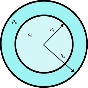
Figure 1: Pictorial representation of the two-layered toy model that we are considering in this section. The density of the outer layer is bigger than that of the inner layer, $\rho_{i}<\rho_{o}$.

We impose that the Misner-Sharp mass function is continuous everywhere. Physically, this means that all the mass of the system is entirely provided by the two layers (i.e. there are not additional shell-like contributions). This implies that we have

$$m(r)=\begin{cases}\frac{4}{3}\pi r^{3}\rho_{i}&r<R_{i}\\ \frac{4}{3}\pi R_{i}^{3}\rho_{i}+\frac{4}{3}\pi\rho_{o}(r^{3}-R_{i}^{3})&R_{i}<r<R\\ M&r>R\end{cases},$$ (23)

together with the constraint:

$$M=\frac{4}{3}\pi R_{i}^{3}\rho_{i}+\frac{4}{3}\pi\rho_{o}(R^{3}-R_{i}^{3}).$$ (24)

As mentioned before, $M$, which represents the ADM mass of the spacetime, cannot surpass the black hole limit: $M<R/2$. The inner radius $R_{i}$ can, at most, range between the centre of the star and the total radius

$$0<R_{i}<R,$$ (25)

since the star would become single-layered in both limits. The outer density $\rho_{o}$ is allowed to vary within the range

$$\rho_{c}<\rho_{o}<\infty,$$ (26)

with $\rho_{c}=3M/4\pi R^{3}$ being the critical density, which corresponds to the limiting case in which $\rho_{i}=\rho_{o}$, i.e., the star has constant density, and therefore it cannot be more compact than what the Buchdahl limit dictates.

Bilayered fluid stars satisfy Israel junction conditions at $R_{i}$ since, by virtue of (8), the discrete jump in $\rho$ between the inner and outer layers translates into a compensatory discontinuity in $p^{\prime}$ that guarantees the continuity of $\Phi^{\prime}$. Consequently, the metric components $g_{tt}$ and $g_{rr}$ are $C^{1}$ and $C^{0}$ functions, respectively. This discontinuous behaviour in the $tt$ component of the stress-energy tensor is of the same kind as the one that occurs at the surface of the star and, therefore, does not carry along the introduction of distributional stress-energy sources of any kind.

The structure of this bilayered fluid sphere is specified by the set of five parameters $\{\rho_{i},R_{i},\rho_{o},R,M\}$. However, not all of the parameters are independent. First of all, since the TOV equation that we are going to solve does not incorporate any additional length scales (such as the one that appears in the semiclassical TOV Carballo-Rubio (2018); Arrechea et al. (2021)), for the numerical problem we can fix one of the parameters as a unit to which the rest are compared. In our case, we will choose $R$ to be that parameter of choice: for all plots, we set $R=1$. Moreover, we have the constraint given in Eq. (24), which reduces the number of independent parameters to four. We will rewrite the parameter $\rho_{i}$ in terms of the other variables

$$\rho_{i}=\frac{3M}{4\pi R_{i}^{3}}+\rho_{o}\left(1-\frac{R^{3}}{R_{i}^{3}}\right),$$ (27)

and take the independent parameters to be $\{M,R_{i},\rho_{o}\}$.

We decide to integrate the TOV equations from the surface of the star towards its centre. Although this is entirely equivalent to outward integrations from a regular centre, our strategy allows to select the compactness of the fluid sphere beforehand, thus proving to be more efficient to search for compactness bounds from the numerical point of view.

Solutions for the functions $p$ and $\Phi$ at the inner layer are straightforward to obtain by integrating the TOV equation (see Appendix A), and fixing the corresponding integration constants in terms of the parameters of the outer layer. Defining the constants $\Phi_{\text{i}}$ and $p_{i}$ as

$$\Phi_{i}=\Phi(R_{i}),\quad p_{i}=p(R_{i}),$$ (28)

we obtain

$$\Phi(r)=\Phi_{i}\log\left[3\left(p_{i}+\rho_{i}\right)-\left(3p_{i}+\rho_{i}\right)\sqrt{\frac{3-8\pi r^{2}\rho_{i}}{3-8\pi R_{i}^{2}\rho_{i}}}~{}\right]-\Phi_{i}\log\left(2\rho_{i}\right),$$ (29)

and

$$p(r)=-\rho+e^{-\Phi(r)+\Phi_{i}}\left[p_{i}+\rho_{i}\right],$$ (30)

for $r<R_{i}$, i.e., inside the inner layer. For the outer layer, instead, the solution can be written as combinations of elliptic functions of cubic roots Wyman (1949), resulting in lengthy and non-illuminating expressions that we omit here but which were obtained and evaluated numerically using the software Mathematica. We have attached a Mathematica notebook containing the pressure, mass, and redshift functions of the outer layers. The query about the maximum compactness allowed by these bilayered toy models reduces to an inquiry about whether there exists a maximum possible value for the total mass $M$ (always below the black hole limit, or $M<R/2$), beyond which there is not any solution in the family preserving a finite and regular pressure function everywhere inside (and equivalently for the redshift function).

We distinguish two situations: the case in which the inner density $\rho_{i}$ is strictly positive, which we explore in detail in Subsec. III.1, with the limiting case $\rho_{i}=0$ presented separately in Subsec. III.2; and the case in which the density of the inner layer is negative, which we discuss in Subsec. III.3. For positive inner densities, the Misner-Sharp function is everywhere positive, and we show that there is a maximum value of the compactness that can be reached around $2M/R\lesssim 0.9706$. For negative inner densities, regions with negative Misner-Sharp mass are allowed in the interior and we find that it allows for stars as compact as desired all the way up to the black hole limit.

III.1 Bilayered stars with positive core densities

Let us begin analyzing the case in which we have $\rho_{i}>0$. The positivity of the right hand side of Eq. (27) imposes a lower bound on $R_{i}$. Explicitly, we have that

$$\left(1-\rho_{c}/\rho_{o}\right)^{1/3}R<R_{i}<R.$$ (31)

We demonstrate that there is an upper bound to the compactness that these stars can achieve, beyond which no regular solutions exist. To establish this, we fix the parameters $R_{i}$ and $\rho_{o}$, and we determine numerically the value of $M_{\infty}(R_{i},\rho_{o})$ that leads to a solution where the central pressure becomes infinite. This solution defines the maximum mass that a sphere with outer density $\rho_{o}$ and inner radius $R_{i}$ can sustain. Spheres with masses below this maximum will have finite pressures throughout, whereas for larger masses, an “infinite pressure surface” emerges at some finite radius of the star $r>0$.

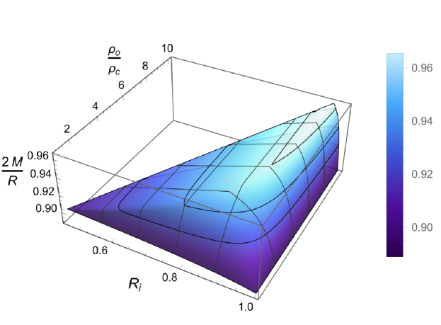
Figure 2: Three dimensional representation of the surface in the $\{R_{i},\rho_{o},M\}$ space corresponding to solutions with an infinite central pressure and $\rho_{i}>0$. Every point on this surface lies above the standard Buchdahl limit $2M/R=8/9$, which is reached in the $\rho_{o}/\rho_{c}\to 1,~{}R_{i}/R\to 1$ limits. Lighter colours denote larger values of $2M/R$, and the black contour lines correspond to the $2M/R=\{0.92,0.94,0.96\}$ planes. This surface can be extended further in the $\rho_{o}/\rho_{c}\gg 1$ direction, where we find a maximum compactness value of $2M/R\approx 0.9706$. We have included a Mathematica notebook containing the pressure, mass, and redshift functions of both the inner and outer layers, as well as this 3D plot, so that any interested reader can visualize it from other angles.

By varying the values of $\rho_{o}$ and $R_{i}$, we can map out a surface in the three-dimensional parameter space $\{R_{i},\rho_{o},M\}$ that precisely represents the value of $M_{\infty}(R_{i},\rho_{o})$ for each pair $\left(R_{i},\rho_{o}\right)$. This surface is shown in Fig. 2. The vertical axis represents the maximum mass allowed for a given $R_{i}$ and $\rho_{o}$. All points on this surface lie between two constant $2M/R$ planes: one above Buchdahl’s limit ($2M/R=8/9$), which it intersects in the limits $\rho_{o}/\rho_{c}\to 1$ and $R_{i}/R\to 1$, and the other below the black hole limit ($2M/R=1$), which it neither intersects nor approaches asymptotically. Extending Fig. 2 in the direction of $\rho_{o}/\rho_{c}\gg 1$, we find the maximum value allowed for the compactness in the model, $C_{\text{max}}$, corresponding to the highest point in the 3D plot. The specific value is

$$C_{\text{max}}=2\sup_{R_{i},\rho_{o}}\frac{M_{\infty}(R_{i},\rho_{o})}{R}\approx 0.9706.$$ (32)

We have constructed a model in which the energy density grows outwards (albeit in a step-function-like fashion) while remaining always positive, thus breaking the second assumption from Buchdahl’s theorem. Despite this, we found it is not possible to arbitrarily approach the black hole limit $2M/R=1$ while keeping the energy density positive everywhere. Instead, the stars considered here display a maximum compactness $C_{\text{max}}$ beyond which the interior becomes singular. Figure 3 shows how this maximum compactness limit scales with the quotient between the outer and critical densities. The maximum appears around the value $\log\left(\rho_{o}/\rho_{c}\right)\approx 11.86$ for $R-R_{i}\approx 2.35\cdot 10^{-6}$. No additional maxima were found in our numerical explorations. We believe that this result is actually robust in the sense that it is independent of the step-function-like profile under consideration, its only model-dependent feature being the specific value of the maximum compactness bound, and not its overall existence.

Figure 3: Maximum compactness limit as a function of the quotient between the energy density of the outer layer and the critical density for stars with $\rho_{i}>0$. A single maximum compactness value of $2M/R\approx 0.9706$, shown in detail, is reached for $\log\left(\rho_{o}/\rho_{c}\right)\approx 11.86$ and $R-R_{i}\approx 2.35\cdot 10^{-6}$. No further maxima were found numerically for larger density values. For $\rho_{o}/\rho_{c}\to 1$, the compactness limit tends to the Buchdahl limit.

III.2 Bilayered stars with vanishing core densities

A particularly illustrative case is the one in which the density of the inner core is zero. We treat it separately because its simplicity allows to find the compactness limit in an easier way. In this situation, the Misner-Sharp mass vanishes everywhere inside the core, and, for a fixed value of the density $\rho_{o}$ and the mass $M$, Eq. (27) enforces the radius $R_{i}$ to be precisely

$$R_{i}=\left(1-\frac{\rho_{c}}{\rho_{o}}\right)^{1/3}R,$$ (33)

where we recall that the expression of $\rho_{c}$ in terms of $\{M,R\}$ is $\rho_{c}=3M/4\pi R^{3}$. This constraint also restricts pressure to be a positive, inwards-increasing monotonic function. This is because, starting from a positive, inwards-growing pressure, the numerator of the TOV equation (9) is only allowed to change sign if $m(r)<0$. Actually, we can explicitly integrate the TOV equation in the inner layer and find the following pressure profile

$$p=\frac{1}{2\pi r^{2}+\kappa},$$ (34)

where $\kappa$ is an arbitrary integration constant whose value is obtained from the matching to the outer layer, i.e.,

$$\kappa=\frac{1}{p_{i}}-2\pi R_{i}^{2}=\frac{1}{p_{i}}-2\pi R^{2}\left(1-\frac{\rho_{c}}{\rho_{o}}\right)^{2/3}.$$ (35)

In Subsection III.1 we noticed that the regular bilayered star with positive density that exhibits the largest possible compactness $C_{\text{max}}$ consisted of a narrow and highly dense shell surrounding an interior of (nearly) vanishing mass. In the present case where the inner core has exactly zero mass, the maximum compactness is attained by the solution (34) with $\kappa=0$, precisely the one that makes the pressure profile diverge exactly at $r=0$. To find this compactness bound, we calculate how $p_{i}$ scales in the $\rho_{o}/\rho_{c}\to\infty$ limit (the limit in which the outer shell is arbitrarily thin) for different values of the compactness.

We have not been able to obtain an analytic expression but we have clearly seen numerically that $p_{i}$ always approaches a constant positive value, which we denote as $P_{i}^{~{}(\text{max})}$, as we vary $\rho_{o}$ while keeping the mass fixed for $\rho_{o}\gg\rho_{c}$. The particular value of $P_{i}^{~{}(\text{max})}$ is also found to increase with the mass, eventually diverging in the $2M/R\to 1$ limit, in agreement with the staticity requirement from Sec. II. From Eq. (35), we see that such divergent behaviour means that $\kappa\leq 0$ when $2M/R\to 1$. By calculating $P_{i}^{~{}(\text{max})}$ for a range of compactness values between the Buchdahl and black hole limits, we find that the compactness for which $\kappa=0$ agrees up to seven decimal places with the maximum compactness value (32) found for bilayered stars with positive density interiors.

In light of these results, we conjecture that given an outwards-increasing, monotonic density profile, there exists an upper bound to the compactness that isotropic stars can achieve, as long as we restrict ourselves to non-negative densities. In order to contrast this hypothesis, we have explored numerically different families of equations of state with similar characteristics that will be reported elsewhere, and in every case we find that there is a maximum available compactness which is actually smaller than the compactness of the toy model examined here. However, by no means we claim that the bilayered star profile is optimal, since, for instance, it is possible to think about this toy model as the limit of a parametric family of density profiles interpolating two constant density regions when the width of the interpolating region vanishes. Currently we lack any arguments to assert that these families—with the interpolation region keeping a finite width—yield less compact objects than the bilayered, step-function model considered here.

Finally, whereas a bound of the form $2m(r)/r<1$ was found in Baumgarte and Rendall (1993) assuming positive energy density and isotropy (see Mars et al. (1996) for an interesting extension to the anisotropic case, where only regularity at $r=0$ and the condition $\rho+p_{r}+2p_{t}\geq 0$ are assumed), our findings here suggest that a more stringent bound could be provided, although we leave the proof (or rebuttal) of this conjecture for future work.

III.3 Bilayered stars with negative densities in the core

We have seen that, by considering a non-negative density profile that increases outward, the upper bound for the compactness exceeds the Buchdahl limit. However, there remains a gap between this new bound and the black hole limit. The next question that we pose is whether allowing the inner density $\rho_{i}$ to take negative values closes that gap, i.e., permits the existence of objects as compact as desired up to the black hole limit. Notice that this relaxation opens the door to violations of the weak (and hence the dominant) energy conditions.

In the case examined previously, we found that the solution which saturates the maximum compactness limit given in Eq. (32) looks (approximately) like a star with all its positive mass stored in a very narrow outer layer. The inner layer, on the contrary, occupies the whole bulk of the star and does not contribute to the mass at all. Such arrangement of the two layers is optimal in the sense that it maximizes the mass of the configuration for a fixed value of the outer density while varying $R_{i}$. A complementary interpretation is the following: the existence of a limit to the compactness implies that there is an optimal size for the outer layer. If this layer were made arbitrarily narrow, it would cause the central pressure to diverge. On the contrary, allowing for a negative density core enables the construction of stars for which the configuration that minimizes the central pressure does not require a very narrow and highly dense outer layer. Examples of these solutions are found by selecting the position of $R_{i}$ in such a way that the pressure remains almost constant inside the core. The compactness of solutions within this second family can be arbitrarily close to the black hole limit. The rest of this subsection is devoted to prove this statement in detail.

Assume, again, a bilayered model with an internal layer of negative density $\rho_{i}$. In order to proceed with the proof, we need to take a step back and consider for a moment the uniform-density, single-layer model ($R_{i}=0$). By inspection of Eqs. (23) and (24), we see that, for $\rho_{o}>\rho_{c}$, the Misner-Sharp mass $m(r)$ takes negative values in the interval $0\leq r<\left(1-\rho_{c}/\rho_{o}\right)^{1/3}R$. Extrapolated to $r=0$, this would point to the existence of a negative delta contribution to the density at the core $r=0$, meaning that the extrapolation of this configuration all the way to the centre of the star is not regular. Here, we only use this irregular configuration to generate the outer layer of the total geometry. In these configurations it is easy to see that the width of the negative-mass region grows with $\rho_{o}$. Now, by the TOV equation (9) we see that, at the surface $r=R$, pressure always increases inwards:

$$p^{\prime}=-\frac{M\rho_{o}}{\left(R-2M\right)R}<0.$$ (36)

Moreover, a negative Misner-Sharp mass can produce a maximum in the pressure at some $r=r_{\text{max}}$, which, by the Eq. (9), corresponds with the point when $m(r_{\text{max}})=-4\pi r_{\text{max}}^{3}p(r_{\text{max}})$. Values of $\rho_{o}$ bigger than a critical value $\rho_{\text{sep}}$ (whose specific value can be found numerically) ensure that it is possible to generate configurations with pressure profiles that are everywhere finite, in the same way that it is done in Arrechea et al. (2021): starting from $p(R)=0$ at the surface, then reaching a maximum value at $r=r_{\text{max}}$, to finally decrease until the centre $r=0$. In the $r\to 0$ limit, we obtain the following behaviour:

$$p\simeq-\rho+k^{-2}\sqrt{\frac{r}{k}},\quad k>0.$$ (37)

As mentioned above, if only one layer is allowed, these configurations display a curvature singularity at $r=0$. However, if we allow for an inner layer with $\rho_{i}<0$ that provides a physical origin to the negative Misner-Sharp mass, then we can find a range of matching radii $R_{-}\leq R_{i}\leq R_{+}$ that guarantees that $p^{\prime}\geq 0$ inside the core and exactly zero at $r=0$, thus yielding a finite and well-defined pressure everywhere. Inside the core, the solutions for the Misner-Sharp mass, redshift, and pressure are given by Eqs. (23–30).

In fact, the two boundaries of this interval $R_{-}$ and $R_{+}$ correspond to the choices of internal radii that make $p_{i}=-\rho_{i}/3$ and $p_{i}=-\rho_{i}$ respectively. These special values will be analyzed in detail in Sec. IV, as well as their connection with ultracompact objects found through semiclassical analyses. On the one hand, for $R_{i}=R_{+}$, the inner core has constant (positive) pressure in a way that guarantees $p+\rho_{i}=0$ everywhere inside the core. The redshift function adopts the simple form

$$\Phi(r)=\Phi_{i}\log\left(\sqrt{\frac{3-8\pi r^{2}\rho_{i}}{3-8\pi R_{i}^{2}\rho_{i}}}\right).$$ (38)

It is straightforward to check that this solution is regular in the range $0\leq r<R_{i}$, since the only divergences in (38) either come from

$$8\pi r^{2}\rho_{i}-3=0,\quad\text{or}\quad 8\pi R_{\text{i}}^{2}\rho_{i}-3=0,$$ (39)

which do not have real roots if $\rho_{i}<0$. On the other hand, the choice $R_{i}=R_{-}$ leads to an inner core that is characterized by a constant redshift function $\Phi(r)=\Phi_{i}$ and which satisfies the condition $3p+\rho_{i}=0$. Figures 4 and 5 show plots of these two solutions with constant-pressure inner cores. For any choice of $R_{i}$ in between those two values, namely $R_{-}<R_{i}<R_{+}$, we obtain regular solutions with $p^{\prime}>0$ inside the core. Regular solutions can also be found for $R_{i}\gtrsim R_{+}$ and for $R_{i}\lesssim R_{-}$ although we do not focus on them here since our aim is only to show that it is possible to find solutions as compact as desired.

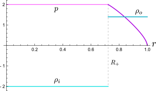
Figure 4: Typical pressure and density profiles for stars displaying a constant-pressure inner layer such that $p+\rho_{i}=0$. The star shown in this Figure has $2M/R=0.99,~{}\rho_{o}=1.4$ and $R_{i}=R_{+}\approx 0.72$. In the limit where the outer layer is infinitesimally thin, these solutions reduce to the AdS star model (see Sec. IV below). It is always possible to find stars belonging to this family for any compactness $2M/R<1$.

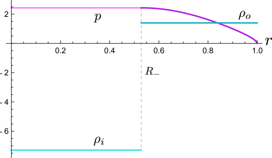
Figure 5: Typical pressure and density profiles for stars displaying a constant-pressure inner layer such that $3p+\rho_{i}=0$. The star shown in this Figure has $2M/R=0.99,~{}\rho_{o}=1.4$ and $R_{i}=R_{-}\approx 0.53$. In the limit where the outer layer is infinitesimally thin, these solutions reduce to the Einstein static star model (see Sec. IV below). It is always possible to find stars belonging to this family for any compactness $2M/R<1$.

Let us now prove that for $R_{i}\in[R_{-},R_{+}]$ the pressure is always bounded in the region $r\in[R_{i},R]$ for any value of $\rho_{o}$ greater than a given value $\rho_{\text{sep}}$. Recall that the density of the inner layer is fixed in terms of the other parameters through Eq. (27). In the $R_{i}\to 0$ limit, it diverges towards negative infinity as

$$\rho_{i}\propto\left(\rho_{c}-\rho_{o}\right)\frac{R^{3}}{R_{i}^{3}},$$ (40)

provided that $\rho_{o}\geq\rho_{\text{sep}}>\rho_{c}$. Since we have chosen $\rho_{o}$ such that pressure in the outer layer remains bounded regardless of the radius $R_{i}$ of the inner layer, and since by moving $R_{i}$ we can construct inner regions with $\rho_{i}\in(-\infty,0)$, there is always an interval $R_{i}\in[R_{-},R_{+}]$ for which $p_{i}/\rho_{i}\in\left[-1,-1/3\right]$. Within this interval of the parameter space, the interior solution for the redshift, given by Eq. (29), is regular, and approaches the solution of Eq. (38) as $R_{i}\to R_{-}$, and the constant solution $\Phi(r)=\Phi_{i}$ as $R_{i}\to R_{+}$. Finally, since $\rho_{\text{sep}}$ exists for every $2M/R<1$, we conclude that, by violating the assumption $\rho_{i}\geq 0$, we can obtain a new family of solutions describing stars with constant-pressure inner layers for which there is no upper compactness bound.

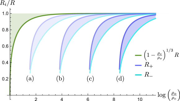
Figure 6: Regions of regular solutions for different compactness values. The shaded green area represents the parameter space for stars with $\rho_{i}>0$, with its boundary is indicated by the green curve. Within this region we find the maximum compactness value $C_{\text{max}}\approx 0.9706$. The shaded blue regions (a), (b), (c) and (d) correspond to regions of the space of parameters (bounded by the curves $R_{+}$ and $R_{-}$) for which we find regular solutions with $2M/R=\left\{0.998,0.9998,0.99998,0.999998\right\}$, respectively. These solutions are necessarily in the $\rho_{i}<0$ region and can be found for any compactness value $2M/R<1$.

As a summary, the main consequence of not constraining the sign of $\rho_{i}$ is that we allow to explore a broader region of the space of parameters $\{R_{i},\rho_{o},M\}$. This is depicted in Fig. 6 where, for some fixed mass value, only solutions inside the green region are allowed to have $\rho_{i}>0$. The green curve $R_{i}=\left(1-\frac{\rho_{c}}{\rho_{o}}\right)^{1/3}R$, where $\rho_{i}=0$, acts as the boundary of this region. Within the green portion of the diagram we find the maximum compactness bound (32). Once we move below said curve, thus allowing for solutions with $\rho_{i}<0$, it is always possible to find broad regions (shaded in blue) of perfectly regular stars, bounded by $R_{+}$ and $R_{-}$. The maximum compactness of these stars can be arbitrarily close to the black hole compactness.

IV AdS Stars and Einstein Static stars

Within the bilayered models with negative energy density at the core, we found two with rather special characteristics whose pressure profiles were plotted in Figs. 4–5. Inspired by these solutions, and considering stars with a compactness close to but below the black hole limit ($8/9<2M/R\sim 1$), we identify configurations with thin external crusts that fall into one of the following two categories:

1. In the core they have a negative density that makes the pressure exactly constant, such that $p(r)=p_{i}=-\rho_{i}$. In the limit in which the outer thick layer becomes infinitesimally thin (distributional), we shall call these stellar configurations AdS stars. See Fig. 4 for a particular example in which the outer shell is thick.

2. In the core they have a negative density that makes the pressure exactly constant, such that $p(r)=p_{i}=-\rho_{i}/3$. In the limit in which the outer thick layer becomes infinitesimally thin (distributional), we shall call these stellar configurations Einstein static stars. See Fig. 5 for a particular example in which the outer shell is thick.

AdS stars are constituted by an anti-de Sitter interior glued through a thin shell to a Schwarzschild exterior. The geometry can be built through a cut and paste procedure with the help of Israel junction conditions. The interesting thing here is that the qualitative behaviour of this ad hoc geometry constructed through this surgery procedure appears naturally within the set of exact regular bilayered models, the only difference being that in that case the shell-like behaviour is absent and the transition between the inside core and the outside is smooth.

An additional feature that AdS and Einstein stars display is that the (distributional) matter supporting the configuration is a non-perfect fluid, e.g., a fluid exhibiting anisotropic pressures. The stress-energy tensor can be expressed in general as:

$$T_{ab}=\rho T_{a}T_{b}+p_{r}R_{a}R_{b}+p_{t}\left(\Theta_{a}\Theta_{b}+\Phi_{a}\Phi_{b}\right),$$ (41)

where $\{T_{a},R_{a},\Theta_{a},\Phi_{b}\}$ represents a tetrad adapted to the symmetry of the problem, and we have introduced the density $\rho$, the radial pressure $p_{r}$, and the tangential pressure $p_{t}$ (notice that the two tangential pressures need to be equal in order for the spherical symmetry to be preserved). The setup that we are considering is depicted in Fig. 7.

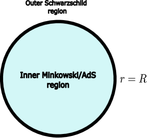
Figure 7: Pictorial representation of the matching of the inner Minkowskian or AdS core with the external Schwarzschild region through a spherically symmetric thin shell.

Let us specify the construction in detail: Take a spherical shell with radius $R$, such that its proper area is $4\pi R^{2}$. Let the spacetime outside the shell be Schwarzschild with a mass $M$, and AdS inside the shell. We denote the Schwarzschild (outside) patch with a $+$ sign, and the AdS (inside) patch with a $-$ sign. The metric reads:

$$ds^{2}_{+}=-f_{+}(r_{+})dt_{+}^{2}+\frac{dr_{+}^{2}}{f_{+}(r_{+})}+r_{+}^{2}d\Omega_{2}^{2},$$ (42)

$$ds^{2}_{-}=-f_{-}(r_{-})dt_{-}^{2}+\frac{dr_{-}^{2}}{f_{-}(r_{-})}+r_{-}^{2}d\Omega_{2}^{2},$$ (43)

with $f_{+}(r_{+})=1-2M/r_{+}$ and $f_{-}(r_{-})=1+\absolutevalue{\lambda}r^{2}$, where $\lambda$ is a real parameter. We locate the shell at $r_{+}=r_{-}=R$. The matching is worked out in detail in Appendix B, and we find that the shell displays a distributional stress-energy tensor with the following densities and pressures:

$$\rho=\sigma\delta(r-R),$$ (44)

$$p_{r}=0,$$ (45)

$$p_{t}=\tilde{p}_{t}\delta(r-R),$$ (46)

with $\sigma$ and $\tilde{p}_{t}$ given by

$$\sigma =\frac{1}{4\pi R}\left(\sqrt{1+|\lambda|R^{2}}-\sqrt{1-\frac{2M}{R}}\right),$$

$$\tilde{p}_{t} =-\frac{1}{8\pi R}\frac{d}{dR}\left(R\sqrt{1+|\lambda|R^{2}}-R\sqrt{1-\frac{2M}{R}}\right).$$ (47)

In the crust of the bilayered model the pressure increases from zero to $p_{i}$. In the distributional limit the pressure exhibits just a jump. The closer the compactness is to 1, the larger this jump in pressure becomes. In this work, we have introduced bilayered models to illustrate their potentiality to generate configurations surpassing the standard Buchdahl limit. However, it is remarkable that the structure of AdS stars is precisely the backbone of the semiclassical stellar solutions found previously in Arrechea et al. (2021, 2024). The only energy-momentum tensor supporting the stellar configurations reported there is that of a perfect fluid of constant density, together with the semiclassical renormalized stress-energy tensor (RSET) that they generate.

In this self-consistent semiclassical solutions there is always a classical positive energy density which in the core is overcome by a negative semiclassical contribution from the RSET. In the limit in which the crust is very thin, these stars can be approximated by AdS stars. In that sense, one can consider AdS stars as idealized models of semiclassical ultracompact stars whose energy momentum tensor is the sum of a perfect fluid and the RSET of a quantum scalar field. It is also interesting to point out that these AdS stars can be interpreted as an inverted version of the well-known gravastar model of Mazur and Mottola Mazur and Mottola (2023), in the sense that gravastars have a de Sitter interior instead of an AdS one.

We also have to mention here the similarities and differences between our AdS stars and the AdS black shells of Danielsson et al. (2017). The biggest difference comes from the compactness. In the AdS black shell construction, the shell is located at around the Buchdahl radius $R=9M/4$. In our case, the shell is located as near to the black hole limit as desired.

Einstein stars are those in which the core has constant positive pressure satisfying $\rho_{i}=-3p_{i}$. We have called them Einstein stars because of their similarities with Einstein static cosmological model Einstein (1917). In that model, a 3-sphere filled with a pressureless dust, representing the matter content of the universe, is counterbalanced by the presence of a cosmological constant. As its cosmological acceleration is zero, we have that $\rho_{\rm total}+3p_{\rm total}=0$. In the cosmological case we have that $\rho_{\rm dust}+\rho_{\Lambda}+3p_{\Lambda}=\rho_{\rm dust}-\Lambda/(4\pi)=0$, with $\Lambda$ the cosmological constant. In the case of our semiclassical stars we have

$$\rho_{\rm class}+\rho_{\rm semiclass}+3p_{\rm semiclass}=0,$$ (48)

with $\rho_{\rm semiclass}$ being the only negative term. Geometrically speaking, these stars have a constant non-zero redshift core.

These models could serve as simple templates of black hole mimickers inspired by semiclassical effects. One central element responsible for both the features of their ringdown Cardoso and Pani (2019) and their associated shadows Ayzenberg et al. (2023) are the redshift and time delay effects suffered by light rays crossing their interiors. While the AdS star has a redshift function that decreases towards the centre, the one associated to the Einstein static star is fully constant. This would result in radically different crossing times for null rays and, in turn, to very different observational signatures both in the electromagnetic and gravitational-wave spectra.

V Anisotropy

To isolate the effect of anisotropy in bypassing the Buchdahl limit, it is convenient to focus on a situation in which there are no violations of energy conditions arising from an interior core. For that purpose, we can analyze a toy model of a shell matching an exterior Schwarzschild spacetime with mass $M$ to an interior flat spacetime (i.e., Schwarzschild with $M=0$). The setup is the same as the one depicted in Fig. 7, but considering the core to be empty instead of AdS. This simply corresponds to setting the AdS constant $\lambda=0$ from previous results, and we find the following energy and tangential pressure densities:

$$\sigma=\frac{1}{4\pi R}\left(1-\sqrt{f_{+}(R)}\right),\quad\tilde{p}_{t}=\frac{1}{16\pi R\sqrt{f_{+}(R)}}\left(-2\sqrt{f_{+}(R)}+2f_{+}(R)+f_{+}^{\prime}(R)R\right).$$ (49)

Given that $\tilde{p}_{t}$ blows up at $R=2M$, and that it goes to zero faster than $\sigma$ as $R\to\infty$, there is a crossover at a given $R=R_{0}$ for which $\sigma=\tilde{p}_{t}$. This means that we can expect violations of energy conditions. In fact, the DEC requires

$$\rho\geq p_{t}.$$ (50)

Given that the two of them have the same distributional behaviour, for our particular example this would imply

$$\sigma\geq\tilde{p}_{t}.$$ (51)

If we plug in the explicit values of $\sigma$ and $\tilde{p}_{t}$ given in Eq. (47), we find the bound:

$$C=\frac{2M}{R}\leq\frac{24}{25}=0.96.$$ (52)

This bound is less stringent than the Buchdahl bound for isotropic situations, $C<8/9\sim 0.888$  Buchdahl (1959). But it is more stringent than the bound that follows from just demanding the positivity of the $g_{rr}$ component of the metric—the black hole limit $C<1$.

In Ivanov (2002), bounds were derived for the maximum redshift that the surfaces of anisotropic stars can have under several assumptions, namely:

$$s=\frac{1}{(1-2M/R)^{1/2}}-1\leq s_{\text{max}},$$ (53)

where the value of the $s_{\text{max}}$ depends on the energy condition that is chosen. In terms of the compactness, we have that the bounds are of the form:

$$\frac{2M}{R}\leq\frac{s_{\text{max}}(s_{\text{max}}+2)}{(1+s_{\text{max}})^{2}}.$$ (54)

In Ivanov (2002), the bounds are derived assuming that the radial pressure is strictly positive (for stability reasons). It is also assumed that $\rho$ is positive and a decreasing function (although it can stay constant for a given interval). Assuming the DEC is obeyed, the upper bound for the redshift found is:

$$s_{\text{max}}^{\text{DEC}}=5.421\rightarrow\frac{2M}{R}\leq 0.974,$$ (55)

whereas imposing the condition that $\rho\geq 2p_{t}$ leads to a more stringent bound:

$$s_{\text{max}}^{\text{SEC}}=3.842\rightarrow\frac{2M}{R}\leq 0.958.$$ (56)

We can compare these bounds with the shell model that we are considering, and we realize that the shell model begins to violate the DEC whenever the compactness is greater than $2M/R=0.96$, which still obeys the bound $2M/R\leq 0.974$ found by Ivanov Ivanov (2002). Further results that put bounds on the compactness of the objects with similar assumptions are the results reported in Barraco et al. (2003); Boehmer and Harko (2006); Lindblom (1984); Urbano and Veermäe (2019). In Barraco et al. (2003), under roughly speaking the same assumptions as Ivanov’s, it is shown that anisotropic models fall into two classes according to whether $p_{r}>p_{t}$ or $p_{t}>p_{r}$. In the case $p_{r}>p_{t}$, they manage to show that the $p_{r}$ function is strictly greater than the one in a fiduciary isotropic model with the same function $m(r)$. This means that these stars cannot be super-Buchdahl; actually, isotropic stars obeying DEC need to be less compact than Buchdahl Barraco and Hamity (2002). Regarding the case $p_{r}<p_{t}$, they show that the radial pressure is always bigger than the one in the fiduciary isotropic model with the same Misner-Sharp mass profile. Imposing the DEC, they derive bounds that are consistent with Ivanov’s. In Boehmer and Harko (2006), under some additional assumptions (about surface density behaviour motivated on physical grounds), slightly sharper bounds are proved. Finally, in Lindblom (1984); Urbano and Veermäe (2019) it is shown that imposing a causality condition, namely that the speed of sound is smaller than the speed of light, there is a maximum compactness that can be reached, which turns out to be below Buchdahl’s limit, namely $2M/R\lesssim 0.768$.

In any case, the simple example exhibited in this section shows that in the absence of energy conditions, anisotropic configurations can be made as compact as desired. Energy conditions set a limit to the compactness, but it is nevertheless far from Buchdahl’s, leaving the door open to having extremely compact objects that are close to forming event horizons, and are even allowed to display photon rings (since for that it is only required that $2M/R>2/3\sim 0.666$).

VI Discussion and future work

In this article, we have presented a comprehensive overview of the ways in which Buchdahl’s limit can be bypassed. We have shown that the relaxation of one (or both) of the main assumptions of Buchdahl’s theorem—namely, the outward decreasing monotonicity of the density profile, and the isotropy of the stress-energy tensor—allows the existence of super-Buchdahl configurations. On the one hand, we have seen that, for non-decreasing (yet everywhere non-negative) density profiles, a new sort of Buchdahl limit seems to arise (as we illustrate for a toy model). We provide compelling evidence that the existence of a less compact bound than the one found in Baumgarte and Rendall (1993) is robust and independent of the model. We also show that as long as we allow negative densities (and hence violations of the weak energy condition), we can make objects as close to the compactness of a black hole as desired. Among the possibilities explored, we derived a particularly simple configuration consisting of an anti-de Sitter interior and a thin shell matching with an exterior Schwarzschild metric, that we have called AdS star, and which bares close resemblance with solutions obtained in semiclassical gravity Arrechea et al. (2024). On the other hand, we also introduced a very simple toy model of an anisotropic shell that allowed us to show that, without further restrictions (such as, e.g., energy conditions), one can conceive objects with compactness arbitrarily close to the black hole limit. The imposition of some energy condition still allows the surpassing of Buchdahl’s limit, but places new upper bounds on the compactness.

Once we allow violations of energy conditions, we need to be careful, since we are opening the door to a plethora of pathological behaviours. For instance, violations of the dominant energy condition are often interpreted as leading to acausal behaviour. The DEC can be understood as representing that the speed of the energy flow of the matter field is always subluminal. This is manifested in a theorem by Hawking Hawking (1970); Hawking and Ellis (2023) which ensures that if the energy-momentum tensor obeys the DEC and it vanishes on a piece of a Cauchy slice, then it vanishes also on the domain of influence of such piece of the Cauchy slice. This can be interpreted as saying that signals obeying the DEC cannot propagate faster than light Wong (2011). However, that the shell (or the constant-density star) itself does not obey the DEC does not necessarily mean that its perturbations are necessarily acausal, since the perturbations with respect to a configuration that violates the DEC are not guaranteed to violate the DEC as well. To put it explicitly, given our configuration with background values of the density and pressure $\bar{\rho},\bar{p}$ that violate the DEC (i.e., $\absolutevalue{\bar{\rho}}\leq\absolutevalue{\bar{p}}$), the perturbations $\delta\rho,\delta p$ do not necessarily obey $\absolutevalue{\delta p}\leq\absolutevalue{\delta\rho}$. Although it might be useful to understand this in terms of a background and a perturbation energy-momentum tensor, such splitting comes with an intrinsic arbitrariness that makes it hard to be precise about in what sense background configurations may violate the DEC without one entering into pathological behaviour for perturbations respecting it. Furthermore, the superluminal behaviour that is tied to violations of the DEC may not necessarily be problematic, as there are examples of situations in which apparently superluminal behaviours do not necessarily entail a pathology Babichev et al. (2008); Geroch (2011); Barceló et al. (2022). We believe that the DEC violation in this case would point to an instability of the background (which in the shell case that we analyze is natural since the object would tend to collapse). The theorems in which the DEC is used, namely, to prove many of the results concerning no-hair theorems, black hole mechanics, and to ensure the well-posedness of the initial value problem in its general formulation Curiel (2017), do not seem to contradict this interpretation.

When we allow non-monotonically decreasing density profiles, we may expect that if the matter content is that of an ordinary fluid, it will display an unstable behaviour, but no energy conditions need to be violated, a priori. If we go further and allow negative energy densities, causally pathological behaviour might arise due to the violation of the WEC. However, if such behaviour of the effective densities and pressures is motivated by an underlying healthy physical mechanism, e.g. semiclassical physics, the pathological behaviour might not arise. In fact, such behaviour is expected from assuming that perturbations with respect to the background constrain the density and pressures in a similar way the background ones do, without this being necessarily the case. For example, a horizonless alternative to GR black holes has recently appeared within semiclassical theories of gravity, where vacuum polarization effects in stars approaching Buchdahl’s limit predict the appearance of outwards increasing (and even negative) energy densities, allowing to bypass Buchdahl’s theorem Arrechea et al. (2024). The bilayered stars proposed in this work capture the core properties of these semiclassical solutions while being devoid of the intricacies of semiclassical analyses, which might foster their phenomenological scrutiny in the future.

Appendix A Fluid spheres in GR

Let us consider the line element in Eq. (1), and the solution corresponding to a perfect fluid with constant density profile, namely:

$$\rho(r)=\begin{cases}\rho_{0}&r\leq R\\ 0&r>R\end{cases}.$$ (57)

For such density profile, the mass function $m(r)$ takes the form

$$m(r)=\begin{cases}\frac{4}{3}\pi r^{3}\rho_{0}&r\leq R\\ \frac{4}{3}\pi R^{3}\rho_{0}&r>R\end{cases},$$ (58)

as a straightforward integration demonstrates, and we have a relation among the parameters $\left(M,R,\rho_{0}\right)$ which is precisely $M=(4/3)\pi R^{3}\rho_{0}$. The pressure and the redshift function also admit explicit expressions given by

$$P(r)=\rho_{0}\left[\frac{(1-2M/R)^{1/2}-(1-2Mr^{2}/R^{3})^{1/2}}{(1-2Mr^{2}/R^{3})^{1/2}-3(1-2M/R)^{1/2}}\right]$$ (59)

and

$$\Phi(r)=\log\left[\frac{3}{2}\left(1-2M/R\right)^{1/2}-\frac{1}{2}\left(1-2Mr^{2}/R^{3}\right)^{1/2}\right].$$ (60)

for $r\leq R$. Everywhere else, the pressure is zero, and the redshift function matches its Schwarzschild counterpart, given in Eq. (4). We can particularize the pressure from Eq. (59) to $r=0$ to realize that the value of the pressure at the core is given by

$$P_{c}=P(0)=\rho_{0}\left[\frac{1-(1-2M/R)^{1/2}}{3(1-2M/R)^{1/2}-1}\right],$$ (61)

which clearly blows up when $R\rightarrow 9M/4$, i.e., as Buchdahl’s limit is approached. Furthermore, it is convenient to rewrite the maximum mass allowed for a star of a given density in terms of the density instead of the radius, namely:

$$M_{\text{Buchdahl}}=\frac{4}{9}R=\frac{4}{9(3\pi)^{1/2}}\rho_{0}^{-1/2}.$$ (62)

Even though the density is not a continuous function because of the jump that it displays at $r=R$, $h$ is still continuous, which is what is required for the proof of Buchdahl’s theorem. In fact, although in this case we are considering a discontinuous function, it is always possible to understand this density profile as a limit that can be approached within a parametric family of smooth $C^{\infty}$ functions $\rho_{\ell}(r)$, such as

$$\rho_{\ell}(r)=\begin{cases}\rho_{0}\,e^{\frac{4\ell^{2}}{R^{2}}+\frac{\ell^{2}}{r(r-R)}}&r<R\\ 0&r>R\end{cases},$$ (63)

which in the limit $\ell\rightarrow 0^{+}$ reduces to a Heaviside function with density $\rho_{0}$ in the interior $r\in(0,R)$ and $0$ in the external region.

Appendix B Fully anisotropic shell matching spherically symmetric spacetimes

Let us consider a static and spherically symmetric spacetime that is foliated in spheres of proper radius $r$. Consider a line element of the form:

$$ds^{2}=-f(r)dt^{2}+\frac{dr^{2}}{f(r)}+r^{2}d\Omega_{2}.$$ (64)

We can consider that the function $f(r)$ is piecewise defined, namely that we have:

$$f(r)=\begin{cases}f_{-}(r)&r<R\\ f_{+}(r)&r>R\end{cases},$$ (65)

where we will consider $f_{+}$ to be that of the Schwarzschild solution $f_{+}(r)=1-2M/r$, with $R\geq 2M$, and $f_{-}(r)$ to be the (A)dS and Minkowski solutions, namely $f_{-}(r)=1+\lambda r^{2}$, being AdS for $\lambda>0$, dS for $\lambda<0$, and Minkowski for $\lambda=0$. We can determine the distributional profile of the energy-momentum tensor that is required to match the two patches using Israel junction conditions.

The first of Israel junction conditions states that the metric needs to be continuous and hence the induced metric on the surface cannot have a discontinuity. The induced metric for the surface (whose components we denote as $h_{ab}$) can be computed from the outside and inside metrics to obtain:

$$ds^{2}_{+}=-f_{+}(R)\left(\frac{dt_{+}}{d\tau}\right)^{2}d\tau^{2}+R^{2}d\Omega_{+,2}^{2},$$ (66)

$$ds^{2}_{-}=-f_{-}(R)\left(\frac{dt_{-}}{d\tau}\right)^{2}d\tau^{2}+R^{2}d\Omega_{-,2}^{2},$$ (67)

where $\tau$ is the proper time of constant $\Theta_{-}$ observers. Continuity of the metric ensures that we can take an orthonormal basis on the surface such that $\Theta^{a}\partial_{a}=\partial_{\theta^{+}}=\partial_{\theta^{-}}$, $\Phi^{a}\partial_{a}=\partial_{\varphi^{+}}=\partial_{\varphi^{-}}$, and

$$f_{+}(R)\left(\frac{dt_{+}}{d\tau}\right)^{2}=f_{-}(R)\left(\frac{dt_{-}}{d\tau}\right)^{2},$$ (68)

which translates into the condition $\sqrt{f_{+}(R)}t_{+}=\sqrt{f_{-}(R)}t_{-}$, choosing the same origin for the time coordinate. The vector tangent to the surface $u=\partial_{\tau}$ can be expressed as:

$$u=\partial_{\tau}=\frac{\partial t_{-}}{\partial\tau}\partial_{t_{-}}=\frac{1}{\sqrt{{f_{-}(R)}}}\partial_{t_{-}},$$ (69)

$$u=\partial_{\tau}=\frac{\partial t_{+}}{\partial\tau}\partial_{t_{+}}=\frac{1}{\sqrt{{f_{+}(R)}}}\partial_{t_{+}}.$$ (70)

We now need $n$, the unit normal vector to the surface which is orthogonal to $u$. It is given by

$$n^{+}_{a}=\frac{1}{\sqrt{f_{+}(r)}}\delta^{r}_{\ a}, n^{-}_{a}=\frac{1}{\sqrt{f_{-}(r+)}}\delta^{r}_{\ a}.$$ (71)

To compute the extrinsic curvature, we need $\nabla_{b}n_{a}$, and we can extract the different components of the extrinsic curvature through

$$K_{\tau\tau}=\nabla_{b}n_{a}u^{b}u^{a},$$ (72)

$$K_{\theta\theta}=\nabla_{b}n_{a}\Theta^{a}\Theta^{b},$$ (73)

$$K_{\Phi\Phi}=\nabla_{b}n_{a}\Phi^{a}\Phi^{b}.$$ (74)

Computed from the outside the extrinsic curvature gives:

$$K^{+}_{\tau\tau}=-\frac{1}{2}\frac{f^{\prime}_{+}}{\sqrt{f_{+}}},$$ (75)

$$K^{+}_{\theta\theta}=\sqrt{f_{+}}R,$$ (76)

$$K^{+}_{\Phi\Phi}=\sqrt{f_{+}}R\sin^{2}\theta,$$ (77)

$$K^{+}=K^{+}_{ab}h^{ab}=\frac{1}{2}\frac{f^{\prime}_{+}}{\sqrt{f_{+}}}+2\frac{\sqrt{f_{+}}}{R},$$ (78)

whereas from the inside we simply need to replace $f_{+}$ by $f_{-}$:

$$K^{-}_{\tau\tau}=-\frac{1}{2}\frac{f^{\prime}_{-}}{\sqrt{f_{-}}},$$ (79)

$$K^{-}_{\theta\theta}=\sqrt{f_{-}}R,$$ (80)

$$K^{-}_{\Phi\Phi}=\sqrt{f_{-}}R\sin^{2}\theta,$$ (81)

$$K^{-}=K^{-}_{ab}h^{ab}=\frac{1}{2}\frac{f^{\prime}_{-}}{\sqrt{f_{-}}}+2\frac{\sqrt{f_{-}}}{R}.$$ (82)

The second junction condition dictates that the jump in the extrinsic curvature is directly proportional to the distributional energy-momentum tensor. Explicitly, we have:

$$8\pi S^{a}_{\ b}=-\left(\left[\left[K^{a}_{\ b}\right]\right]-\left[\left[K\right]\right]\delta^{a}_{\ b}\right),$$ (83)

where we have introduced the notation $\left[\left[\mathcal{O}\right]\right]=\mathcal{O}^{+}-\mathcal{O}^{-}$, representing precisely the jump in the extrinsic curvatures. We can compute it to find:

$$\left[\left[K^{\tau}_{\ \tau}\right]\right]=\frac{1}{2}\frac{f^{\prime}_{+}}{\sqrt{f_{+}}}-\frac{1}{2}\frac{f^{\prime}_{-}}{\sqrt{f_{-}}},$$ (84)

$$\left[\left[K^{\theta}_{\ \theta}\right]\right]=\frac{\sqrt{f_{+}}}{R}-\frac{\sqrt{f_{-}}}{R},$$ (85)

$$\left[\left[K^{\Phi}_{\ \Phi}\right]\right]=\frac{\sqrt{f_{+}}}{R}-\frac{\sqrt{f_{-}}}{R},$$ (86)

$$\left[\left[K\right]\right]=\frac{1}{2}\left(\frac{f^{\prime}_{+}}{\sqrt{f_{+}}}-\frac{f^{\prime}_{-}}{\sqrt{f_{-}}}\right)+2\frac{\sqrt{f_{+}}-\sqrt{f_{-}}}{R}.$$ (87)

From this expression we can determine $S^{a}_{\ b}$. For our purpose, it is interesting that we can express the tensor as that of a perfect fluid,

$$S_{ab}=\sigma u_{a}u_{b}+\tilde{p}_{t}\left(h_{ab}+u_{a}u_{b}\right),$$ (88)

where $\sigma$ and $\tilde{p}_{t}$ represent the surface energy density and the surface tangential pressure, respectively, and are given by

$$\sigma =\frac{1}{4\pi R}\left(\sqrt{f_{-}(R)}-\sqrt{f_{+}(R)}\right),$$ (89)

$$\tilde{p}_{t} =\frac{\sqrt{f_{+}(R)}-\sqrt{f_{-}(R)}}{8\pi R}+\frac{1}{16\pi R}\left(\frac{f^{\prime}_{+}}{\sqrt{f_{+}}}-\frac{f^{\prime}_{-}}{\sqrt{f_{-}}}\right).$$ (90)

References

- Collmar et al. (1998) W. Collmar, N. Straumann, S. K. Chakrabarti, G. ’t Hooft, E. Seidel, and W. Israel, in Black Holes: Theory and Observation, edited by F. W. Hehl, C. Kiefer, and R. J. Metzler (Springer Berlin Heidelberg, Berlin, Heidelberg, 1998) pp. 481–489.
- Abramowicz et al. (2002) M. A. Abramowicz, W. Kluzniak, and J.-P. Lasota, Astron. Astrophys. 396, L31 (2002), arXiv:astro-ph/0207270 .
- Carballo-Rubio et al. (2022) R. Carballo-Rubio, V. Cardoso, and Z. Younsi, Phys. Rev. D 106, 084038 (2022), arXiv:2208.00704 [gr-qc] .
- Nauenberg (2008) M. Nauenberg, Journal for the History of Astronomy 39, 297 (2008).
- Chandrasekhar (1931) S. Chandrasekhar, The London, Edinburgh, and Dublin Philosophical Magazine and Journal of Science 11, 592 (1931), https://doi.org/10.1080/14786443109461710 .
- Chandrasekhar (1931) S. Chandrasekhar, Astrophys. J. 74, 81 (1931).
- Oppenheimer and Volkoff (1939) J. R. Oppenheimer and G. M. Volkoff, Phys. Rev. 55, 374 (1939).
- Nilsson and Uggla (2000) U. S. Nilsson and C. Uggla, Annals of Physics 286, 292 (2000).
- Buchdahl (1959) H. A. Buchdahl, Phys. Rev. 116, 1027 (1959).
- Bondi (1964) H. Bondi, Proceedings of the Royal Society of London. Series A. Mathematical and Physical Sciences 282, 303 (1964).
- Wald (1984) R. M. Wald, General Relativity (Chicago Univ. Pr., Chicago, USA, 1984).
- Schwarzschild (1916) K. Schwarzschild, in Sitzungsberichte der Königlich Preussischen Akademie der Wissenschaften zu Berlin (1916) pp. 424–434.
- Mazur and Mottola (2023) P. O. Mazur and E. Mottola, Universe 9, 88 (2023).
- Danielsson et al. (2017) U. H. Danielsson, G. Dibitetto, and S. Giri, JHEP 10, 171 (2017), arXiv:1705.10172 [hep-th] .
- Arrechea et al. (2021) J. Arrechea, C. Barceló, R. Carballo-Rubio, and L. J. Garay, Phys. Rev. D 104, 084071 (2021), arXiv:2105.11261 [gr-qc] .
- Arrechea et al. (2024) J. Arrechea, C. Barceló, R. Carballo-Rubio, and L. J. Garay, Phys. Rev. D 109, 104056 (2024), arXiv:2310.12668 [gr-qc] .
- Martin-Garcia et al. (2021) J. M. Martin-Garcia, A. García-Parrado, A. Stecchina, B. Wardell, C. Pitrou, D. Brizuela, et al., http://www.xact.es (latest version Oct. 2021).
- Misner and Sharp (1964) C. W. Misner and D. H. Sharp, Phys. Rev. 136, B571 (1964).
- Hernandez and Misner (1966) J. Hernandez, Walter C. and C. W. Misner, Astrophys. J. 143, 452 (1966).
- Bardeen (1968) J. Bardeen, in Proceedings of the 5th International Conference on Gravitation and the Theory of Relativity (1968) p. 87.
- Hayward (1996) S. A. Hayward, Phys. Rev. D53, 1938 (1996), arXiv:gr-qc/9408002 [gr-qc] .
- Dymnikova (1992) I. Dymnikova, Gen. Rel. Grav. 24, 235 (1992).
- Lindblom (1984) L. Lindblom, Astrophys. J. 278, 364 (1984).
- Ivanov (2002) B. V. Ivanov, Phys. Rev. D 65, 104011 (2002), arXiv:gr-qc/0201090 .
- Barraco et al. (2003) D. E. Barraco, V. H. Hamity, and R. J. Gleiser, Phys. Rev. D 67, 064003 (2003).
- Boehmer and Harko (2006) C. G. Boehmer and T. Harko, Class. Quant. Grav. 23, 6479 (2006), arXiv:gr-qc/0609061 .
- Urbano and Veermäe (2019) A. Urbano and H. Veermäe, JCAP 04, 011 (2019), arXiv:1810.07137 [gr-qc] .
- Carballo-Rubio (2018) R. Carballo-Rubio, Phys. Rev. Lett. 120, 061102 (2018), arXiv:1706.05379 [gr-qc] .
- Wyman (1949) M. Wyman, Phys. Rev. 75, 1930 (1949).
- Baumgarte and Rendall (1993) T. W. Baumgarte and A. D. Rendall, Classical and Quantum Gravity 10, 327 (1993).
- Mars et al. (1996) M. Mars, M. M. Martin-Prats, and J. M. M. Senovilla, Phys. Lett. A 218, 147 (1996), arXiv:gr-qc/0202003 .
- Einstein (1917) A. Einstein, Sitzungs. König. Preuss. Akad. , 142 (1917).
- Cardoso and Pani (2019) V. Cardoso and P. Pani, Living Rev. Rel. 22, 4 (2019), arXiv:1904.05363 [gr-qc] .
- Ayzenberg et al. (2023) D. Ayzenberg et al., (2023), arXiv:2312.02130 [astro-ph.HE] .
- Barraco and Hamity (2002) D. Barraco and V. H. Hamity, Phys. Rev. D 65, 124028 (2002).
- Hawking (1970) S. Hawking, Commun. Math. Phys. 18, 301 (1970).
- Hawking and Ellis (2023) S. W. Hawking and G. F. R. Ellis, The Large Scale Structure of Space-Time, Cambridge Monographs on Mathematical Physics (Cambridge University Press, 2023).
- Wong (2011) W. W.-Y. Wong, Class. Quant. Grav. 28, 215008 (2011), arXiv:1011.3029 [math-ph] .
- Babichev et al. (2008) E. Babichev, V. Mukhanov, and A. Vikman, JHEP 02, 101 (2008), arXiv:0708.0561 [hep-th] .
- Geroch (2011) R. Geroch, AMS/IP Stud. Adv. Math. 49, 59 (2011), arXiv:1005.1614 [gr-qc] .
- Barceló et al. (2022) C. Barceló, J. E. Sánchez, G. García-Moreno, and G. Jannes, Eur. Phys. J. C 82, 299 (2022), arXiv:2201.11072 [gr-qc] .
- Curiel (2017) E. Curiel, Einstein Stud. 13, 43 (2017), arXiv:1405.0403 [physics.hist-ph] .