Market Making without Regret

Nicolò Cesa-Bianchi Università degli Studi di Milano, Milano, Italy Politecnico di Milano, Milano, Italy Tommaso Cesari University of Ottawa, Ottawa, Italy Roberto Colomboni Università degli Studi di Milano, Milano, Italy Politecnico di Milano, Milano, Italy Luigi Foscari Università degli Studi di Milano, Milano, Italy Vinayak Pathak Independent researcher
Abstract

We consider a sequential decision-making setting where, at every round $t$, a market maker posts a bid price $B_{t}$ and an ask price $A_{t}$ to an incoming trader (the taker) with a private valuation for one unit of some asset. If the trader’s valuation is lower than the bid price, or higher than the ask price, then a trade (sell or buy) occurs. If a trade happens at round $t$, then letting $M_{t}$ be the market price (observed only at the end of round $t$), the maker’s utility is $M_{t}-B_{t}$ if the maker bought the asset, and $A_{t}-M_{t}$ if they sold it. We characterize the maker’s regret with respect to the best fixed choice of bid and ask pairs under a variety of assumptions (adversarial, i.i.d., and their variants) on the sequence of market prices and valuations. Our upper bound analysis unveils an intriguing connection relating market making to first-price auctions and dynamic pricing. Our main technical contribution is a lower bound for the i.i.d. case with Lipschitz distributions and independence between prices and valuations. The difficulty in the analysis stems from the unique structure of the reward and feedback functions, allowing an algorithm to acquire information by graduating the “cost of exploration” in an arbitrary way.

Keywords: Regret minimization, online learning, market making, first-price auctions, dynamic pricing.

1 Introduction

Trading in financial markets is a crucial activity that helps keep the world’s economy running, and several players, including hedge funds, prop trading firms, investment banks, central banks, and retail traders participate in it daily. While every actor has their own objective function (for example, a hedge fund wants to maximize profit whereas a central bank wants to keep inflation in check), at a fundamental level, trading can be viewed as a stochastic control problem where agents want the state to evolve so as to maximize their objective function. In this work we focus on market makers, i.e., traders whose job is to facilitate other trades to happen. One way to do so is by broadcasting, at all times, a price (bid) at which they are willing to buy, and a price (ask) at which they are willing to sell the asset being traded. This way when a buyer (seller) arrives, they do not have to wait for a seller (buyer) to be able to perform a transaction. A market where it is easy to make trades is called liquid, and liquidity is a desirable property for any kind of market. A market maker thus provides an essential service by increasing the liquidity of the market, and collects compensation for it by (among other ways) ensuring that the bid is always smaller than the ask, thus making a profit proportional to the difference between the bid and the ask. Market making is challenging, and a lot of thought goes into making it profitable, see [38] for an overview. A major risk that a market maker has to deal with, called adverse selection, is the risk that your counterpart is an informed trader who knows something about the future direction of the price movement. For example, an informed trader who knows that an asset is soon about to become cheaper will sell it to you thus forcing you to buy something whose price crashes. One way to mitigate this risk is to immediately offload your positions elsewhere. This strategy can be profitable if, for example, you have access to two markets for the same asset where one market is less liquid than the other. You can be a market maker for the less liquid market while offloading your positions in the more liquid one. We call this strategy “market making with instant clearing”.

1.1 Related works

Perhaps closest to our work is the paper [10], where they compete against a class of $N$ constant-spread dynamic strategies. Although we also compete with constant-spread (static) strategies, their results are not directly comparable to ours for several reasons. First, in their model the only unknown parameter is the market price, whose change from step to step is adversarial yet bounded by a known quantity. As the market price is revealed at the end of each step, their utility function at time $t$ is fully known at the end of step $t$. This implies that their model has a full information feedback, which yields a regret of order $\sqrt{T\ln N}$ against the best constant-spread strategy. In our setting, instead, we compete against a continuum of strategies parametrized by ask-bid pairs. This forces us to simultaneously control estimation and approximation error. Moreover, and crucially, our market model does not have a full information feedback, as our reward function depends on the taker’s private valuations which remain unknown. Hence, we need to carefully exploit the structure of the reward function to compensate for the missing information. Please see Section 5 for an extensive list of related works.

1.2 Our contributions

Adversarial IID
General Lip General Lip IV Lip+IV
Realistic $T$ $T^{\nicefrac{{2}}{{3}}}$ $T$ $T^{\nicefrac{{2}}{{3}}}$ $T^{\nicefrac{{2}}{{3}}}$ $T^{\nicefrac{{2}}{{3}}}$
Full $T$ $\sqrt{T}$ $\sqrt{T}$ $\sqrt{T}$ $\sqrt{T}$ $\sqrt{T}$
Table 1: A summary of the regret guarantees we prove for each variant of the online market-making problem. All the rates are optimal up to logarithmic factors.

We study the question of market making with instant clearing in an online learning setup. Here, trading happens in discrete time steps and an unknown stochastic process governs the prices of the asset being traded as well as the private valuations assigned to the asset by market participants (see details in Section 2). The market maker is an online learning algorithm that posts a bid and an ask at the beginning of each time step and receives some feedback at the end of the time step. We are interested in controlling the regret suffered by this learner at the end of $T$ time steps. We consider two feedback models. In both models, the learner can see the price (called the market price) at which they are able to offload their position at the end of the time step. However, in the realistic feedback model, they can only see whether their bid or the ask (or neither) got successfully traded, whereas in the full feedback model, they also get to see the private valuations of their counterpart in the trade. For each feedback model, we consider the i.i.d. setting, where the unknown stochastic process is i.i.d., as well as the adversarial setting, where no such assumption is made on the process. Our results are summarized in Table 1.

In the realistic feedback model, we make the following contributions.

  1. 1.

    We design the M3 (meta-)algorithm (Algorithm 2) and prove a $\mathcal{O}(T^{\nicefrac{{2}}{{3}}})$ upper bound on its regret under the assumption that either the cumulative distribution functions of the takers’ valuations are Lipschitz or the sequence of market prices and takers’ valuations are i.i.d. with market prices being independent of taker’s valuations (Theorem 3.3).

  2. 2.

    Our main technical contribution is a lower bound of order $\Omega(T^{\nicefrac{{2}}{{3}}})$ that matches M3’s upper bound, and holds even under the simultaneous assumptions that the sequence of market prices and takers’ valuations is i.i.d., admits Lipschitz cumulative distribution functions, and is such that market prices are independent of takers’ valuations (Theorem 3.4).

  3. 3.

    We then investigate the necessity of assuming either Lipschitzness of the cumulative distribution function of the takers’ valuations or independence of market values and takers’ valuations. We prove that, if both assumptions are dropped, learning is impossible in general, even when market values and takers’ valuations are i.i.d. (Theorem 3.5).

Lastly, we discuss the full-feedback case to flesh out the impact of limited feedback on learning rates and learnability. We show that learning is impossible in the adversarial setting (Theorem 4.1), while it is possible to achieve an $\mathcal{O}(\sqrt{T})$ regret rate when market values and takers’ valuations are i.i.d. (Theorem 4.3), or when the cumulative distribution functions of takers’ valuations are Lipschitz (Theorem 4.4). This rate is unimprovable, even if the three previous assumptions hold at the same time (Theorem 4.2).

1.3 Techniques and challenges

We now move on to describe the main technical challenges encountered when proving our results.

Upper bounds. First observe that the learner’s action space (i.e., the set of ask/bid pairs) is the two dimensional set $\{(b,a)\in[0,1]^{2}\mid b\leq a\}$. If market prices and takers’ valuations are both generated adversarially, standard bandit approaches typically require Lipschitzness (or the weaker one-side Lipschitzness) of the reward function, a property that is unfortunately missing in our setting. We can recover Lipschitzness (in expectation) by smoothing111I.e., by assuming that their cumulative distribution function is Lipschitz. the taker’s valuations, while the market prices remain adversarial. Under the smoothness assumption, the problem can be seen as an instance of $2$-dimensional Lipschitz bandits, and a black-box application of existing continuous bandits techniques [60] would give us only a suboptimal regret rate $\mathcal{O}(T^{\nicefrac{{3}}{{4}}})$. Using a different approach that exploits the structure of our feedback and reward functions, we manage to effectively reduce the dimensionality of the problem by $1$, thus obtaining an improved (and optimal, as discussed later) $\mathcal{O}(T^{\nicefrac{{2}}{{3}}})$ regret rate, see Theorem 3.2.

The previous result is based on discretizing the action space and exploiting the Lipschitzness of the expected reward function provided by the smoothness assumption, together with the available feedback (which is sufficient to reconstruct bandit feedback). Can discretization be used to obtain the same rate when smoothed adversarial valuations are replaced by a different, yet natural, assumption? In Section 3.1 we consider an i.i.d. setting with independence between market prices and private valuations. Although this assumption does not provide Lipschitzness (not even in expectation), we show that the same algorithm as before has a regret again bounded by $\mathcal{O}(T^{\nicefrac{{2}}{{3}}})$. However, the analysis relies on a different observation: although we cannot guarantee that the reward of all actions is well approximated by that of a corresponding point in the grid, we can guarantee the weaker property that the expected reward of the best actions are approximated by the expected reward of a point in the grid, which is sufficient to prove the desired rate.

Lower bounds. A first roadblock in constructing regret lower bounds is that, in contrast to standard multi-armed bandits problems, we can control the distribution of the feedback and the expected reward functions only indirectly, through the joint distribution of market prices and valuations. In particular, there are constraints on the types of reward functions we can design, and it is non-trivial to design underlying joint distributions of market prices and valuations whose corresponding expected reward functions have the desired properties.

Another challenge is that the learner’s feedback in our setting is richer than bandit feedback. Therefore, even if we could encode our expected reward functions in hard multi-armed bandit instances, we would not be able to rely on the same arguments. A similar reason prevents us from applying the known $\Omega(T^{\nicefrac{{2}}{{3}}})$ lower bounds for dynamic pricing and first-price auctions, two problems that turn out to be closely related to ours. Proving the optimality of the $T^{\nicefrac{{2}}{{3}}}$ rate in the i.i.d. setting under the assumptions of smoothness and independence of market prices and taker’s valuations is a highly nontrivial task which represents the main technical contribution of this work.

To understand the complexity of proving a lower bound, we now compare the trade-offs between regret and amount of feedback in hard instances of our setting and of other related settings. The three main ingredients in the standard lower bound approach for online learning with partial feedback are:

  • Hard instances, constructed as “$\varepsilon$-perturbations” of a base instance obtained by slightly altering the base distributions of some of the random variables drawn by the environment.

  • The amount of information acquired when playing an action, quantified by the Kullback-Leibler (KL) divergence between the distribution of the feedback obtained when selecting the action in the perturbed instance and the corresponding feedback distribution when selecting the action in the base instance—the higher, the better.

  • The regret of an action, simply measured by the expected instantaneous regret of the action in the perturbed instance—the smaller, the better.

In hard instances of $K$-armed bandits, an arm is drawn uniformly at random from a $K$-sized set and assigned an expected reward $\varepsilon$-higher than the other arms in the set. Selecting an optimal arm costs zero regret and provides $\Theta(\varepsilon^{2})$ bits of information. Selecting a non-optimal arm, instead, provides no information and costs $\varepsilon$ regret [6]. This implies that any algorithm has only one way to acquire information about an arm, i.e., to play that arm. A similar situation occurs in other settings, including those with continuous decision spaces.

Refer to caption
Figure 1: Utility (in red) and amount of acquired information (in blue) in a hard instance of the classic multi-armed bandit problem with a finite set of arms (on the left) and in a hard instance of the first-price auctions problem with a continuous set of bids (on the right). Both quantities are maximized at the same point. In particular where there is no perturbation, there is no information and some amount of reward, otherwise the KL can grow up to a quantity of order $\varepsilon^{2}$ and the utility can grow by a quantity of order $\varepsilon$.

For example, to acquire information about a bid in the standard hard instance of first-price auctions, the only reasonable option is to post that price, incurring regret $\Theta(\varepsilon)$ if the arm is non-optimal and acquiring $\Theta(\varepsilon^{2})$ bits of information if the arm is optimal [25]. See Figure 1 for a pictorial representation of the expected reward and KL divergence in said hard instances.

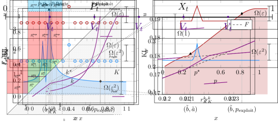
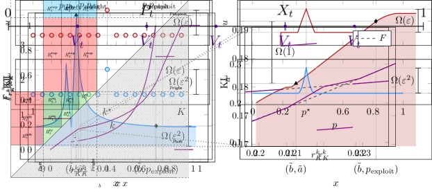
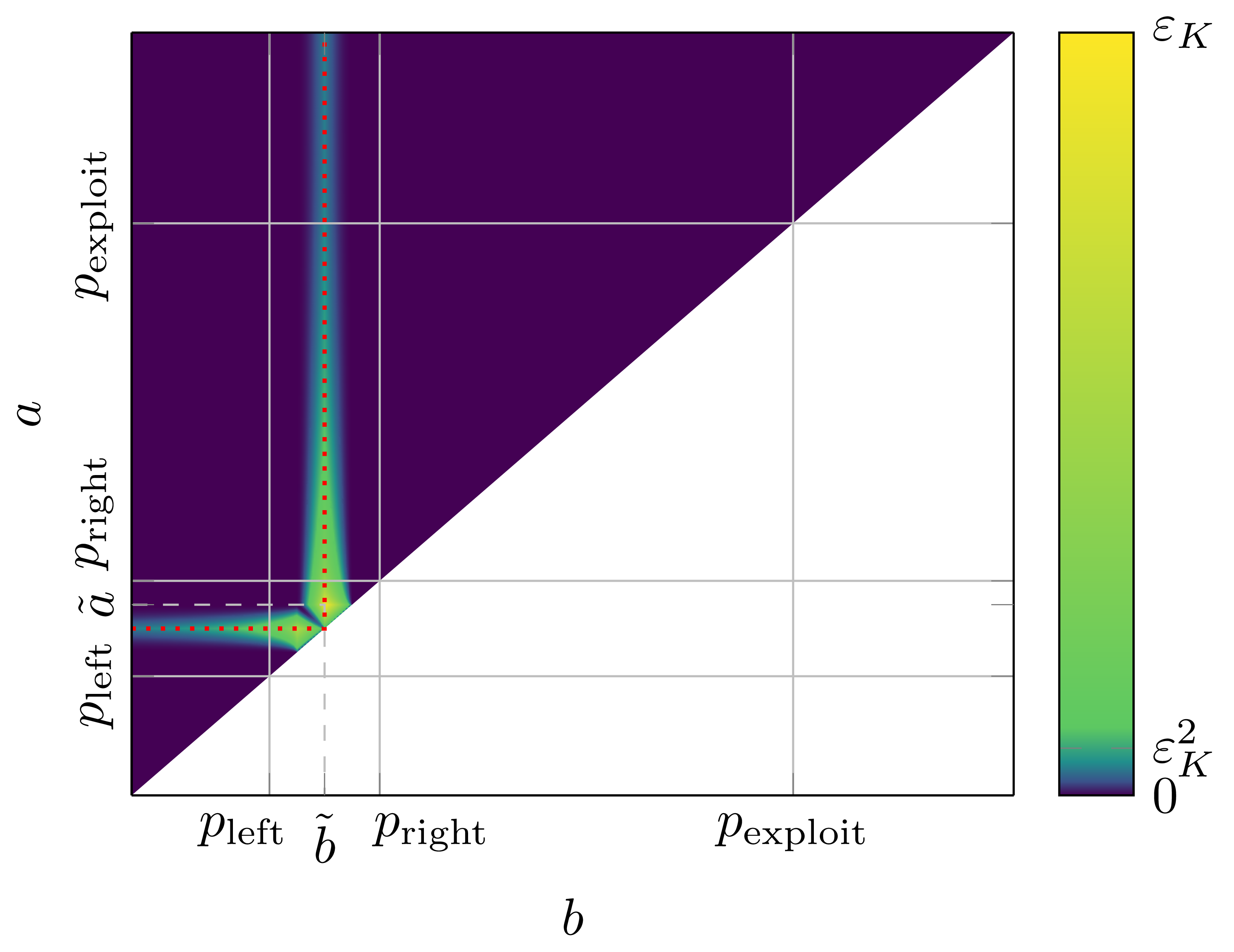
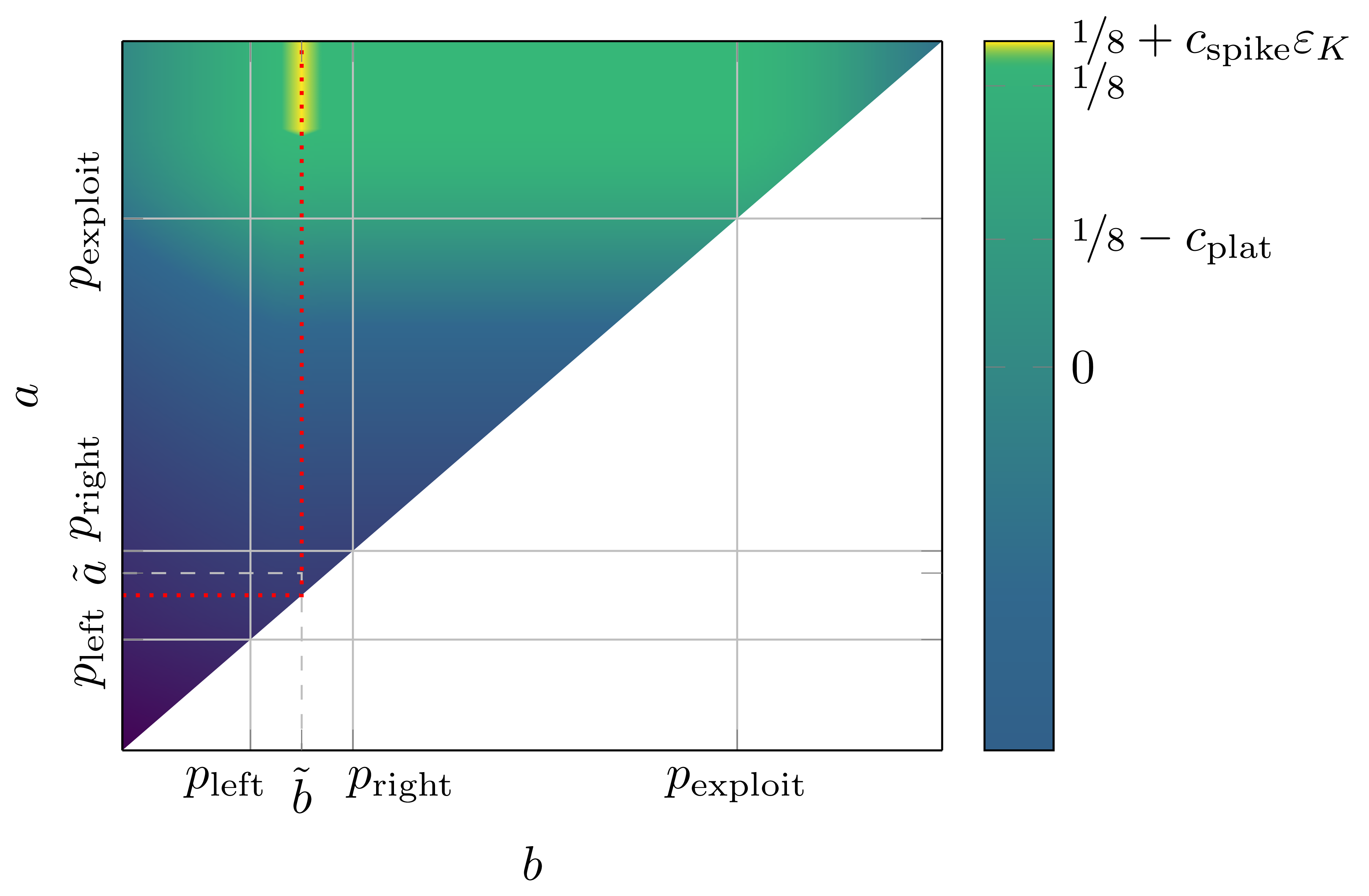
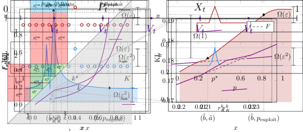
In a hard instance of market-making, a price $b^{\star}$ is drawn uniformly at random from a known finite set of bid prices and the bid/ask pair $(b^{\star},1)$ is given a reward $\varepsilon$-higher than the other bid/ask pairs of the form $(b^{\prime},1)$. The amount of information and corresponding regret of each pair of prices $(b,a)$ can be visualized by looking at the qualitative plots in Figure 3. Note that there are uncountably many ways to determine if a pair of prices $(b,1)$ is optimal: playing any pair in the non-blue area of the left plot in Figure 3 allows to modulate the amount of exploration, with the points that yield the highest quality feedback being the ones with low reward and high regret (for a plot representing the growth of the amount of feedback and the corresponding reward as a function of the pair $(b,a)$ taken along a representative path, see Figure 4). Consequently, the exploration-exploitation trade-off consists in first choosing whether to exploit with some pair $(b,1)$, or instead pick another potentially optimal pair $(b^{\prime},1)$ to explore, then choosing from an uncountable set of options $(b^{\prime\prime},a^{\prime\prime})$ how much regret one is willing to suffer in order to acquire more information about the optimality of $(b^{\prime},1)$.222 The situation is even more complex because, in the realistic feedback model, pairs $(b,a)$ allow to test for the optimality not just of the pair $(b,1)$, but also of the pair $(a,1)$. To build a lower bound, we then need to consider all possible ways a learner can handle these multiple trade-offs between information and regret. To the best of our knowledge, this is the first lower bound for a problem exhibiting a continuum of trade-offs between reward and feedback. As our setting is arguably simple, we expect the same phenomenon to occur in other applications of online learning to digital markets. We solve the problem by partitioning the action space into finitely many elements (or clusters) that can be further grouped in three macro-categories: “get high regret but (potentially) lots of information”, “get (potentially) small regret but also little information”, and clearly suboptimal actions where we “get some regret and no information”. We then analyze an algorithm in terms of how many times it selects an action from each cluster, using similar techniques for all clusters belonging to the same macro-category. We believe that the clustering technique developed in this work could be helpful in tackling similar lower bounds exhibiting a continuum of trade-offs that might appear in future works applying online learning to digital market problems.

We close this section with a last remark. When investigating the necessity of the assumptions of smoothness and independence of valuations and prices, if both these assumptions are dropped, an intriguing needle-in-a-haystack phenomenon arises: by devising discrete entangled takers’ valuations and market prices distributions, we show that it becomes impossible for the learner to determine an optimal action within a finite horizon in a continuum of potentially optimal actions.

2 Setting

In online market making, the action space of the maker is the upper triangle $\mathcal{U}\coloneqq\bigl{\{}(b,a)\in[0,1]^{2}\,:\,b\leq a\bigr{\}}$, enforcing the constraint that a bid price $b$ is never larger than the corresponding ask price $a$. For an overview of the notation, see Table 2, in Appendix A. The utility of the market maker, for all $(b,a)\in\mathcal{U}$ and $m,v\in[0,1]$, is

$$u(b,a,m,v)\coloneqq(m-b)\cdot\underbrace{\mathbb{I}\{b\geq v\}}_{\text{Maker buys}}+\;(a-m)\cdot\underbrace{\mathbb{I}\{a<v\}}_{\text{Maker sells}}\;,$$ (1)

where $v$ is the taker’s private valuation and $m$ is the market price.333The choice of buying when $b\geq v$ and selling when $a<v$ models a taker that is slightly more inclined to sell rather than buy: in this case, the taker is willing to sell even when their valuation is exactly equal to the bid. This choice is completely immaterial for the results that follow and is merely done for the sake of simplicity. All the results we present still hold if trades happen according to a similar rule but with a taker that is slightly more inclined to buy rather than sell (i.e., if a trade occurs whenever $b>v$ or $a\leq v$) or if this inclination changes arbitrarily whenever a new taker comes at any new time step.

for time t=1,2,𝑡12t=1,2,\ldots  do
      Taker arrives with a private valuation $V_{t}\in[0,1]$;
      Maker posts bid/ask prices $(B_{t},A_{t})\in\mathcal{U}$;
      Feedback $\mathbb{I}\{B_{t}\geq V_{t}\}$ and $\mathbb{I}\{A_{t}<V_{t}\}$ is revealed;
      if $B_{t}\geq V_{t}$ then Maker buys and pays $B_{t}$ to Taker;
      else if $A_{t}<V_{t}$ then Maker sells (short) and is paid $A_{t}$ by Taker;
      else no trade happens;
      The market price $M_{t}\in[0,1]$ is revealed;
     
     if Maker bought from Taker then Maker offloads to Market at price $M_{t}$;
     else if Maker sold (short) to Taker then Maker buys from Market at price $M_{t}$;
      Maker’s utility is $U_{t}(B_{t},A_{t})\coloneqq u(B_{t},A_{t},M_{t},V_{t})$;
     
tradingprotocol]a:trading-protocol
Trading protocol 1 Market making with instant clearing and realistic feedback

Our online market making protocol is specified in LABEL:a:trading-protocol. At every round $t$, a taker arrives with a private valuation $V_{t}\in[0,1]$ and the maker posts bid/ask prices $(B_{t},A_{t})\in\mathcal{U}$. If $B_{t}<V_{t}\leq A_{t}$ (i.e., if the taker is not willing to sell nor to buy at the proposed bid/ask prices), then no trade happens. If $B_{t}\geq V_{t}$ (buy) or $A_{t}<V_{t}$ (sell), a trade happens. At the end of each round, the maker observes the market price $M_{t}$ and the type of trade (buy, sell, none) that took place in that round. The maker’s utility is determined by $U_{t}(B_{t},A_{t})\coloneqq u(B_{t},A_{t},M_{t},V_{t})$. Hence, any (possibly randomized) learning strategy for the maker at time $t$ is a map that takes all previous feedback $\big{\{}\big{(}\mathbb{I}\{B_{\tau}\geq V_{\tau}\},\mathbb{I}\{A_{\tau}<V_{\tau}\},M_{\tau}\big{)}\big{\}}_{\tau<t}$, plus some optional random seeds, to a (random) pair $(B_{t},A_{t})$ of bid/ask prices in $\mathcal{U}$.

The maker’s goal is to minimize, for any time horizon $T\in\mathbb{N}$, the regret after $T$ time steps:

$$R_{T}\coloneqq\sup_{(b,a)\in\mathcal{U}}\mathbb{E}\left[\sum_{t=1}^{T}U_{t}(b,a)\right]-\mathbb{E}\left[\sum_{t=1}^{T}U_{t}(B_{t},A_{t})\right]\;,$$

where the expectations are with respect to the (possible) randomness of the market prices, takers’ valuations, and (possibly) the internal randomization of the algorithm. Note that the supremum is not attained in general, because of the strict inequality in one of the two indicator functions in Equation 1.

Types of feedback.

We call the feedback received in the protocol above “realistic feedback”. In a real market, we very rarely have access to the private valuation $V_{t}$ of the taker and thus it is safe to assume that the learner only gets to observe $\mathbb{I}\{B_{t}\geq V_{t}\}$ and $\mathbb{I}\{A_{t}<V_{t}\}$. Still, one can imagine scenarios where additional information about $V_{t}$ is sometimes available. In this spirit and with the goal of contrasting the effect of partial feedback on learnability and learning rates, it is of theoretical interest to study what happens in the other extreme, the full feedback scenario, where the learner gets to observe the value of $V_{t}$ (in addition to $M_{t}$) at the end of each time step $t$. There might be other interesting feedback models between realistic and full that we leave for future work.

3 Realistic feedback

Note that the utility of our market-making problem can be viewed as the sum of the utilities of two related sub-problems: the first addend in (1) corresponds to the utility in a repeated first-price auction problem with unknown valuations, while the second addend corresponds to the utility in a dynamic pricing problem with unknown costs. This suggests trying to use two algorithms for the two problems to solve our market-making problem. However, in our problem we have the further constraint that the bid we propose in the first-price auction is no greater than the price we propose in the dynamic pricing problem. This constraint prevents us from running directly two independent no-regret algorithms for the two different problems because the bid/ask pair produced this way may violate the constraint. To cope with this obstruction, we present a meta-algorithm (Algorithm 2) that takes as input two algorithms for the two sub-problems and combines them to post pairs in $\mathcal{U}$ while preserving the respective guarantees. We now formally introduce the two related problems and build the explicit reduction.

Repeated first-price auctions with unknown valuations.

Consider the following online problem of repeated first-price auctions where the learner only learns the valuation of the good they are bidding on after the auction is cleared. At any time $t$, two $[0,1]$-valued random variables $Z_{t}$ and $H_{t}$ are generated and hidden from the learner: $Z_{t}$ is the current valuation of the good and $H_{t}$ is the highest competing bid for the good, both unknown to the learner at the time of bidding. Then, the learner bids an amount $X_{t}\in[0,1]$ and wins the bid if and only if their bid is higher than or equal to the highest competing bid. The utility of the learner is $Z_{t}-X_{t}$ if they win the auction and zero otherwise. Finally, the valuation of the good $Z_{t}$ and the indicator function $\mathbb{I}\{X_{t}\geq H_{t}\}$ (representing whether or not the learner won the auction) are revealed to the learner.

The goal is to minimize, for any time horizon $T\in\mathbb{N}$, the regret after $T$ time steps

$$R^{\mathrm{fpa}}_{T}\coloneqq\sup_{x\in[0,1]}\mathbb{E}\left[\sum_{t=1}^{T}(Z_{t}-x)\cdot\mathbb{I}\{x\geq H_{t}\}\right]-\mathbb{E}\left[\sum_{t=1}^{T}(Z_{t}-X_{t})\cdot\mathbb{I}\{X_{t}\geq H_{t}\}\right]\;,$$

where the expectations are taken with respect to the (possible) randomness of $(Z_{1},H_{1}),\dots(Z_{T},H_{T})$ and the (possible) internal randomization of the algorithm that outputs the bids $X_{1},\dots,X_{T}$.

The same setting was studied in [25], but with different feedback models.

Dynamic pricing with unknown costs.

Consider the following online problem of dynamic pricing where the learner only learns the current cost of the item they are selling after interacting with the buyer. At any time $t$, two $[0,1]$-valued random variables $C_{t}$ and $W_{t}$ are generated and hidden from the learner: $C_{t}$ is the current cost of the item, and $W_{t}$ is the buyer’s valuation for the item. Then, the learner posts a price $P_{t}\in[0,1]$ and the buyer buys the item if and only if their valuation is higher than the posted price. The utility of the learner is $P_{t}-C_{t}$ if the buyer bought the item and zero otherwise. Finally, the cost of the item $C_{t}$ and the indicator function $\mathbb{I}\{P_{t}<W_{t}\}$ (representing whether or not the buyer bought the item) are revealed to the learner.

The goal is to minimize, for any time horizon $T\in\mathbb{N}$, the regret after $T$ time steps

$$R^{\mathrm{dp}}_{T}\coloneqq\sup_{p\in[0,1]}\mathbb{E}\left[\sum_{t=1}^{T}(p-C_{t})\cdot\mathbb{I}\{p<W_{t}\}\right]-\mathbb{E}\left[\sum_{t=1}^{T}(P_{t}-C_{t})\cdot\mathbb{I}\{P_{t}<W_{t}\}\right]\;,$$

where the expectations are taken with respect to the (possible) randomness of $(C_{1},W_{1}),\dots(C_{T},W_{T})$ and the (possible) internal randomization of the algorithm that outputs the posted prices $P_{1},\dots,P_{T}$.

Dynamic pricing is generally studied under the assumption that costs are known and all equal to zero, and assuming that the buyer buys whenever their evaluation is greater than or equal to the posted price—see, e.g., [46, 26, 52, 51].

First-price auctions plus dynamic pricing implies market making.

In this section, we introduce a meta-algorithm that combines two sub-algorithms, one for repeated first-price auctions with unknown valuations and one for dynamic pricing with unknown costs. This way, we obtain an algorithm for market-making and we show in Theorem 3.1 that its regret can be upper bounded by the sum of the regrets of the two sub-algorithms (in two corresponding sub-problems). The idea of our meta-algorithm M3 (Algorithm 2) begins with the observation that the utility of the market maker is a sum of two terms that correspond to the utilities of the learner in first-price auctions and dynamic pricing respectively. This suggests maintaining two algorithms in parallel, one to determine buying prices and one to determine selling prices. M3 then enforces the constraint that buying prices should be no larger than selling prices by swapping the recommendations of the two sub-algorithms whenever they generate corresponding bid/ask prices that would violate the constraint. Finally, M3 leverages the available feedback $\left(\mathbb{I}\{B_{t}\geq V_{t}\},\mathbb{I}\{A_{t}<V_{t}\},M_{t}\right)$ at time $t$ to reconstruct and relay back to the two sub-algorithms the counterfactual feedback they would have observed if the swap didn’t happen (i.e., if the learner always posted the prices determined by the sub-algorithms).

input: Algorithm $\mathcal{A}$ for repeated first-price auctions with unknown valuations
Algorithm $\mathcal{A}^{\prime}$ for dynamic pricing with unknown costs
for time t=1,2,𝑡12t=1,2,\ldots  do
      Let $X_{t}$ be the output of $\mathcal{A}$ at time $t$ and let $P_{t}$ be the output of $\mathcal{A}^{\prime}$ at time $t$;
      if $X_{t}\leq P_{t}$ then  let $B_{t}:=X_{t}$ and $A_{t}:=P_{t}$;
      else if $X_{t}>P_{t}$ then  let $B_{t}:=P_{t}$ and $A_{t}:=X_{t}$;
      Post buying/selling prices $(B_{t},A_{t})$ and observe feedback $\mathbb{I}\{B_{t}\geq V_{t}\}$, $\mathbb{I}\{A_{t}<V_{t}\}$, and $M_{t}$;
      if $X_{t}\leq P_{t}$ then  feed $(\mathbb{I}\{B_{t}\geq V_{t}\},M_{t})$ back to $\mathcal{A}$ and $(\mathbb{I}\{A_{t}<V_{t}\},M_{t})$ to $\mathcal{A}^{\prime}$;
      else if $X_{t}>P_{t}$ then  feed $(1-\mathbb{I}\{A_{t}<V_{t}\},M_{t})$ back to $\mathcal{A}$ and $(1-\mathbb{I}\{B_{t}\geq V_{t}\},M_{t})$ to $\mathcal{A}^{\prime}$;
     
Algorithm 2 M3 (Meta Market Making)

The next result shows that the regret of M3 is upper bounded by the sum of the regrets of the two sub-algorithms.

Theorem 3.1.

Let $T\in\mathbb{N}$. Suppose that $(M_{t},V_{t})_{t\in[T]}$ is a $[0,1]^{2}$-valued stochastic process.

  • $\bullet$

    Let $\mathcal{A}^{\mathrm{fpa}}$ be an algorithm for repeated first-price auctions with unknown valuations and let $R^{\mathrm{fpa}}_{T}$ be its regret over the sequence $(Z_{t},H_{t})_{t\in[T]}\coloneqq(M_{t},V_{t})_{t\in[T]}$ of unknown valuations and highest competing bids.

  • $\bullet$

    Let $\mathcal{A}^{\mathrm{dp}}$ be an algorithm for dynamic pricing with unknown costs and let $R^{\mathrm{dp}}_{T}$ be its regret over the sequence $(C_{t},W_{t})_{t\in[T]}\coloneqq(M_{t},V_{t})_{t\in[T]}$ of unknown costs and buyers’ valuations.

Then, in the realistic-feedback online market-making problem, the regret of M3 run with parameters $\mathcal{A}^{\mathrm{fpa}}$ and $\mathcal{A}^{\mathrm{dp}}$ over the sequence $(M_{t},V_{t})_{t\in[T]}$ of market values and takers’ valuations satisfies

$$R_{T}\leq R^{\mathrm{fpa}}_{T}+R^{\mathrm{dp}}_{T}\;.$$
Proof.

First, notice that the feedback received by the two algorithms is equal to the feedback they would have retrieved in the corresponding instances regardless of whether or not the prices are swapped. Hence, the regret guarantees of the prices posted by the two algorithm on the original sequence still hold true. Notice that, for each $t\in\mathbb{N}$, we have that

$$(\textrm{I}_{t})\coloneqq U_{t}(B_{t},A_{t})\geq(M_{t}-X_{t})\mathbb{I}\{X_{t}\geq V_{t}\}+(P_{t}-M_{t})\mathbb{I}\{V_{t}>P_{t}\}\eqqcolon(\textrm{II}_{t})\;.$$

In fact, if $X_{t}\leq P_{t}$ the two quantities are equal because $B_{t}=X_{t}$ and $A_{t}=P_{t}$. Instead, if $P_{t}<X_{t}$ (Figure 2), then $B_{t}=P_{t}$ and $A_{t}=X_{t}$, and a direct computation shows that

  • if $V_{t}\leq P_{t}$ then $(\textrm{I}_{t})=M_{t}-P_{t}>M_{t}-X_{t}=(\textrm{II}_{t})$

  • if $P_{t}<V_{t}\leq X_{t}$ then $(\textrm{I}_{t})=0>P_{t}-X_{t}=(\textrm{II}_{t})$

  • if $X_{t}<V_{t}$ then $(\textrm{I}_{t})=X_{t}-M_{t}>P_{t}-M_{t}=(\textrm{II}_{t})\;.$

It follows that

$\displaystyle R_{T}$ $\displaystyle=\sup_{(b,a)\in\mathcal{U}}\mathbb{E}\left[\sum_{t=1}^{T}U_{t}(b,a)\right]-\mathbb{E}\left[\sum_{t=1}^{T}(\mathrm{I}_{t})\right]\leq\sup_{(b,a)\in\mathcal{U}}\mathbb{E}\left[\sum_{t=1}^{T}U_{t}(b,a)\right]-\mathbb{E}\left[\sum_{t=1}^{T}(\mathrm{II}_{t})\right]$
$\displaystyle\leq\sup_{b\in[0,1]}\mathbb{E}\left[\sum_{t=1}^{T}(M_{t}-b)\mathbb{I}\{b\geq V_{t}\}\right]-\mathbb{E}\left[\sum_{t=1}^{T}(M_{t}-X_{t})\mathbb{I}\{X_{t}\geq V_{t}\}\right]$
$\displaystyle\qquad+\sup_{a\in[0,1]}\mathbb{E}\left[\sum_{t=1}^{T}(a-M_{t})\mathbb{I}\{a<V_{t}\}\right]-\mathbb{E}\left[\sum_{t=1}^{T}(P_{t}-M_{t})\mathbb{I}\{P_{t}<V_{t}\}\right]=R^{\mathrm{fpa}}_{T}+R^{\mathrm{dp}}_{T}\;.\qed$
Refer to caption
Figure 2: Possible relative positioning of $V_{t}$ with respect to $P_{t}$ and $X_{t}$, when $P_{t}<X_{t}$.

3.1 $T^{\nicefrac{{2}}{{3}}}$ upper bound (Adversarial+Lip) or (IID+IV)

Consider the problem of repeated first-price auctions with unknown valuations. Since the feedback received at the end of each round allows to compute the utility of the learner, a natural strategy is to simply discretize the interval $[0,1]$ and run a bandit algorithm on the discretization. The pseudo-code of this simple meta-algorithm can be found in Algorithm 3. The following theorem shows its guarantees.

input: Number of arms $K\in\{2,3,\dots\}$, Algorithm $\mathcal{A}$ for $K$-armed bandits
initialization: Let $q_{k}\coloneqq\frac{k-1}{K-1}$, for all $k\in[K]$
for time t=1,2,𝑡12t=1,2,\ldots do
      Let $I_{t}\in[K]$ be the output of $\mathcal{A}$ at time $t$;
      Post bid $X_{t}\coloneqq q_{I_{t}}$ and observe feedback $Z_{t}$ and $\mathbb{I}\{X_{t}\geq H_{t}\}$;
      Compute utility $(Z_{t}-X_{t})\cdot\mathbb{I}\{X_{t}\geq H_{t}\}$ and feed it back to $\mathcal{A}$;
     
Algorithm 3 Discretized Bandits for First Price Auctions
Theorem 3.2.

In the repeated first-price auctions with unknown valuations problem, let $T\in\mathbb{N}$ be the time horizon and let $(Z_{t},H_{t})_{t\in[T]}$ be the $[0,1]^{2}$-valued stochastic process representing the sequence of valuations and highest competing bids. Assume that one of the two following conditions is satisfied:

  1. 1.

    For each $t\in[T]$, the cumulative distribution function of $H_{t}$ is $L$-Lipschitz, for some $L>0$.

  2. 2.

    The process $(Z_{t},H_{t})_{t\in[T]}$ is i.i.d. and, for each $t\in[T]$, the two random variables $Z_{t}$ and $H_{t}$ are independent of each other.

Then, for any $K\geq 2$ and any $K$-armed bandit algorithm $\mathcal{A}$, letting $R^{K}_{T}$ be the regret of $\mathcal{A}$ when the reward at any time $t\in[T]$ of any arm $k\in[K]$ is $(Z_{t}-q_{k})\mathbb{I}\{q_{k}\geq H_{t}\}$, the regret of Algorithm 3 run with parameters $K$ and $\mathcal{A}$ satisfies $R_{T}\leq R_{T}^{K}+\frac{\widetilde{L}+1}{2(K-1)}T\;,$ with $\widetilde{L}=L$ (resp., $\widetilde{L}=1$) if Item 1 (resp., Item 2) holds. In particular, if $T\geq 2$, by choosing $K\coloneqq\lceil T^{\nicefrac{{1}}{{3}}}\rceil+1$ and, as the underlying learning procedure $\mathcal{A}$, an adapted version of Poly INF [2], the regret of Algorithm 3 run with parameters $K$ and $\mathcal{A}$ satisfies $R_{T}\leq c\cdot T^{\nicefrac{{2}}{{3}}}\;,$ where $c\leq L+50$ (resp. $c\leq 51$) if Item 1 (resp., Item 2) holds.

A completely analogous theorem can be proved for Algorithm 4 for the problem of dynamic pricing with unknown costs (see Theorem B.1 in Appendix B).

input: Number of arms $K\in\{2,3,\dots\}$, Algorithm $\mathcal{A}$ for $K$-armed bandits
initialization: Let $q_{k}\coloneqq\frac{k-1}{K-1}$, for all $k\in[K]$
for time t=1,2,𝑡12t=1,2,\ldots do
      Let $I_{t}\in[K]$ be the output of $\mathcal{A}$ at time $t$;
      Post price $P_{t}\coloneqq q_{I_{t}}$ and observe feedback $C_{t}$ and $\mathbb{I}\{P_{t}<W_{t}\}$;
      Compute utility $(P_{t}-C_{t})\cdot\mathbb{I}\{P_{t}<W_{t}\}$ and feed it back to $\mathcal{A}$;
     
Algorithm 4 Discretized Bandits for Dynamic Pricing

Next, we use Theorem 3.2 and Theorem B.1 to show that the regret of M3 is bounded by $\mathcal{O}(T^{\nicefrac{{2}}{{3}}})$.

Theorem 3.3.

In the realistic-feedback online market-making problem, let $T\in\mathbb{N}$ be the time horizon and let $(M_{t},V_{t})_{t\in[T]}$ be the $[0,1]^{2}$-valued stochastic process representing the sequence of market prices and takers’ valuations. Assume that one of the two following conditions is satisfied:

  1. 1.

    For each $t\in[T]$, the cumulative distribution function of $V_{t}$ is $L$-Lipschitz, for some $L>0$.

  2. 2.

    The process $(M_{t},V_{t})_{t\in[T]}$ is i.i.d. and, for each $t\in[T]$, the two random variables $M_{t}$ and $V_{t}$ are independent of each other.

Then, let $K\coloneqq\lceil T^{\nicefrac{{1}}{{3}}}\rceil+1$, let $\mathcal{A}$ be the instance of Algorithm 3 that uses Poly INF as described in Theorem 3.2, and $\mathcal{A}^{\prime}$ be the instance of Algorithm 4 that uses Poly INF as described in Theorem B.1. Then the regret of M3 (Algorithm 2) run with parameters $\mathcal{A}$ and $\mathcal{A}^{\prime}$ satisfies $R_{T}\leq cT^{\nicefrac{{2}}{{3}}}$ with $c\leq 2L+100$ (resp., $c\leq 102$) if Item 1 (resp., Item 2) holds.

Proof.

By Algorithm 2, the regret of M3 is upper bounded by the regret of a repeated first-price auctions problem with unknown valuations plus a dynamic pricing problem with unknown costs. Plugging in the bounds from Theorem 3.2 and Theorem B.1, we get the required result. ∎

3.2 $T^{\nicefrac{{2}}{{3}}}$ lower bound (IID+Lip+IV)

In this section we prove the main lower bound, showing that no algorithm can achieve a regret better than $\Omega(T^{\nicefrac{{2}}{{3}}})$ even when the sequence of market values and taker’s valuations is i.i.d. with a smooth distribution, and market values and taker’s valuations are independent of each other.

Theorem 3.4.

In the realistic-feedback online market-making problem, for each $L\geq 8$, each time horizon $T\geq 42$, and each (possibly randomized) algorithm for realistic-feedback online market making, there exists a $[0,1]^{2}$-valued i.i.d. sequence $(M_{t},V_{t})_{t\in[T]}$ of market values and taker’s valuations such that for each $t\in[T]$ the two random variables $M_{t}$ and $V_{t}$ are independent of each other, they admit an $L$-Lipschitz cumulative distribution function, and the regret of the algorithm over the sequence $(M_{t},V_{t})_{t\in[T]}$ is lower bounded by $R_{T}\geq cT^{\nicefrac{{2}}{{3}}}$ where $c$ is a constant and $c\geq 10^{-6}$.

Before presenting the full proof of this theorem, we give a high-level description of its key ideas. The first step is to build a base joint distribution over market values and takers’ valuations such that the expected utility function of the learner is maximized over an entire segment of pairs of prices $(b,1)$, for $b$ that belongs to some interval (which are instances where it is never optimal to sell). Then, we partition this set of maximizers into $K=\Theta(T^{\nicefrac{{1}}{{3}}})$ segments with the same size and build $K$ perturbations of the base distribution such that, in each one of these perturbations, the corresponding expected utilities have a small $\varepsilon=\Theta(1/K)$-spike inside one of these subsegments. To obtain this result, we draw market values uniformly on $\bigl{[}\frac{7}{8},1\bigr{]}$ and define a more involved distribution for the takers’ valuations (see Figure 5 for the plot of one of these perturbed distributions over takers’ valuations). From here, we start with a simple observation: If we content ourselves with proving a lower bound for algorithms that play exclusively bid/ask pairs of the form $(b,1)$, our problem reduces to repeated first-price auctions with unknown valuations. In this simplified problem, the learner has to essentially locate an $\varepsilon$-spike present in one of $\nicefrac{{1}}{{\varepsilon}}$ locations. Therefore, the learner can either refuse to locate the spike, consequently paying an overall $\Theta(\varepsilon T)$ regret in the worst case, or invest $\Omega(\nicefrac{{1}}{{\varepsilon^{2}}})$ rounds444Given that the KL divergence between the base distribution of the feedback of points in a perturbed region and the perturbed distribution of the feedback of the same points is $O(\varepsilon^{2})$, a standard information-theoretic argument shows that $\Omega(\nicefrac{{1}}{{\varepsilon^{2}}})$ samples of points in a region are needed to determine if the spike is present in that region. in trying to locate each one of the $\nicefrac{{1}}{{\varepsilon}}$ potential spikes, paying $\Omega(\varepsilon)$ each time a point in the wrong region is selected, for an overall regret of $\Omega\bigl{(}\frac{1}{\varepsilon^{2}}\cdot\frac{1}{\varepsilon}\cdot\varepsilon\bigr{)}=\Omega(\nicefrac{{1}}{{\varepsilon^{2}}})$. The hardest instance is when $\varepsilon T=\nicefrac{{1}}{{\varepsilon^{2}}}$, i.e., when $\varepsilon=T^{\nicefrac{{1}}{{3}}}$. In this case, no matter what the learner decides, they will always pay at least $\Omega(\varepsilon T)=\Omega(\nicefrac{{1}}{{\varepsilon^{2}}})=\Omega(T^{\nicefrac{{2}}{{3}}})$ regret. The problem becomes substantially more delicate in our setting because, now, to explore a potential action $(b,1)$, the learner has access to uncountably more options $(b,a)$ (see Figure 3).

Refer to caption
Refer to caption
Figure 3: The heat maps of the amount of information (on the left) and the expected utilities (on the right) obtained by selecting pairs of prices in a hard instance we construct in our $\Omega(T^{\nicefrac{{2}}{{3}}})$ lower bound for i.i.d. smooth instances with market values independent of takers’ valuations (Theorem 3.4). To distinguish the optimal region with reward of (at least) $\nicefrac{{1}}{{8}}+c_{\mathrm{spike}}\varepsilon_{K}$ (the yellow region at the top of the right plot) from the suboptimal region with reward $\nicefrac{{1}}{{8}}$, one could play any point in the non-blue horizontal and vertical regions on the left plot. Note that the pairs that yield the highest amount of feedback (the two small yellow neighborhoods close to the diagonal on the left plot) give highly suboptimal rewards, which are at least $c_{\textrm{plat}}=\Omega(1)$ below $\nicefrac{{1}}{{8}}$.

This complicates things because, in usual online learning lower bounds, the worst-case regret of an algorithm is analyzed by counting how many times the algorithm plays exploiting and exploring arms, then quantifying how much information was gathered from the exploration and summing over all exploring arms. This strategy is hardly implementable in our setting because each exploiting pair $(b,1)$ can be explored with uncountably many other arms $(b^{\prime},s^{\prime})$, and each one trades off some reward to gather some amount of feedback (see Figure 4)—for example, one could post two prices $(b,b+\theta)$, for some small $\theta>0$ paying $\Omega(1)$ regret to obtain much higher quality feedback than if they played $(b,1)$ ($\varepsilon$ vs $\varepsilon^{2}$ KL-divergence information).

Refer to caption
Figure 4: The amount of information (on the left) and the corresponding expected utility (on the right) as a function of pairs of prices $(b,a)$, with $(b,a)$ following the red dashed line in Figure 3 starting at the left boundary of the horizontal non-blue region at the point $(0,\widetilde{b})$, moving horizontally up to the diagonal, then vertically up to the optimal pairs $(b^{\star},1)$, parameterized by a real number $x$. The points $(\widetilde{b},\widetilde{a})$ and $(\widetilde{b},p_{\mathrm{exploit}})$ illustrate how regions of high reward and regions of high information do not coincide, in fact the cost of gathering more information (play $(\widetilde{b},\widetilde{a})$ instead of $(\widetilde{b},p_{\mathrm{exploit}})$) can be a constant $\Omega(1)$ in the reward. On the other hand, a high-reward play can cost $\Omega(\epsilon)$ in the amount of information (but still gathering a quantity $\Omega(\epsilon^{2})$).

We circumvent this problem by clustering the action set $\mathcal{U}$ into finitely many disjoint subsets (see Figure 6) and analyzing all points belonging to the same set in a similar way. This way, we are able to prove that no matter how an algorithm decides to play, there will always be instances where it has to pay a regret of order at least $\Omega(T^{\nicefrac{{2}}{{3}}})$.

Proof.

Fix $T\geq 42$. We define the following constants that will be used in the proof.

$\displaystyle K$ $\displaystyle\coloneqq\bigl{\lceil}T^{\nicefrac{{1}}{{3}}}\bigr{\rceil}$ $\displaystyle\varepsilon_{K}$ $\displaystyle\coloneqq\nicefrac{{1}}{{16K}}$ $\displaystyle\forall k\in[K],\ r_{K}^{k}$ $\displaystyle\coloneqq\nicefrac{{3}}{{16}}+\left(k-\nicefrac{{1}}{{2}}\right)\varepsilon_{K}$
$\displaystyle p_{\textbf{left}}$ $\displaystyle\coloneqq\nicefrac{{3}}{{16}}$ $\displaystyle p_{\textbf{right}}$ $\displaystyle\coloneqq\nicefrac{{1}}{{4}}$ $\displaystyle p_{\textbf{exploit}}$ $\displaystyle\coloneqq\nicefrac{{3}}{{4}}$
$\displaystyle c_{\textbf{plat}}$ $\displaystyle\coloneqq\nicefrac{{1}}{{32}}$ $\displaystyle c_{\textbf{spike}}$ $\displaystyle\coloneqq\nicefrac{{1}}{{72}}$

Define the density

$$f\colon[0,1]\to[0,\infty)\;,\qquad x\mapsto\frac{8}{9}\cdot\mathbb{I}_{\left[0,\frac{3}{16}\right]}(x)+\frac{1}{8}\frac{1}{\left(\frac{15}{16}-x\right)^{2}}\cdot\mathbb{I}_{\left(\frac{3}{16},\frac{3}{4}\right]}(x)+\frac{8}{3}\cdot\mathbb{I}_{\left(\frac{3}{4},\frac{7}{8}\right]}(x)\;,$$
Refer to caption

; Refer to caption;

Figure 5: Above, the perturbed density $f_{r^{k}_{K},\varepsilon_{K}}(x)$ and below, the perturbed cumulative density $F_{r^{k}_{K},\varepsilon_{K}}(x)$ with $K=3$, $k=2$, the highlighted portions show the effects of the perturbation $\Lambda_{r^{k}_{K},\varepsilon_{K}}$ on the density function $f(x)$ and on the cumulative distribution function $F(x)$ respectively. The dotted lines represent the base functions.

so that the corresponding cumulative distribution function $F$ satisfies, for each $x\in[0,1]$,

$$F(x)=\frac{8}{9}x\cdot\mathbb{I}_{\left[0,\frac{3}{16}\right]}(x)+\frac{1}{8}\frac{1}{\frac{15}{16}-x}\cdot\mathbb{I}_{\left(\frac{3}{16},\frac{3}{4}\right]}(x)+\frac{8}{3}\left(x-\frac{1}{2}\right)\cdot\mathbb{I}_{\left(\frac{3}{4},\frac{7}{8}\right]}(x)+\mathbb{I}_{\left(\frac{7}{8},1\right]}(x)\;.$$ (2)

We define a family of perturbations parameterized by the set $\Xi\coloneqq\{(r,\varepsilon)\in[\frac{3}{16},\frac{11}{16}]\times[0,1]\mid\frac{3}{16}\leq r-\frac{\varepsilon}{2}\leq r+\frac{\varepsilon}{2}\leq\frac{11}{16}\}$; for each $(r,\varepsilon)\in\Xi$, define $g_{r,\varepsilon}\coloneqq\frac{1}{9}\cdot\mathbb{I}_{[r-\frac{\varepsilon}{2},r]}-\frac{1}{9}\cdot\mathbb{I}_{(r,r+\frac{\varepsilon}{2}]}$ and $f_{r,\varepsilon}\coloneq f+g_{r,\varepsilon}$. Notice that for each $(r,\varepsilon)\in\Xi$ the function $f_{r,\varepsilon}$ is still a density function whose corresponding cumulative distribution function $F_{r,\varepsilon}$ satisfies, for each $x\in[0,1]$,

$$F_{r,\varepsilon}(x)=F(x)+\frac{\varepsilon}{18}\Lambda_{r,\varepsilon}(x)\;,$$

where $\Lambda_{r,\varepsilon}$ is the tent function of height $1$ and width $\varepsilon$ centered in $r$, i.e., the function defined, for each $x\in\mathbb{R}$, by

$$\Lambda_{r,\varepsilon}(x)\coloneqq\left(1-\frac{2}{\varepsilon}(r-x)\right)\cdot\mathbb{I}_{\left[r-\frac{\varepsilon}{2},r\right]}(x)+\left(1-\frac{2}{\varepsilon}(x-r)\right)\cdot\mathbb{I}_{\left(r,r+\frac{\varepsilon}{2}\right]}(x)\;.$$

Note that $F_{r,\varepsilon}$ is $4$-Lipschitz; indeed, for each $(b,a)\in\mathcal{U}$,

$$\left\lvert F_{r,\varepsilon}(a)-F_{r,\varepsilon}(b)\right\rvert=\int^{a}_{b}f_{r,\varepsilon}(x)\,\,\mathrm{d}x=\max_{c\in[b,a]}f_{r,\varepsilon}(c)(a-b)\leq\left(\max_{c^{\prime}\in[0,1]}f(c^{\prime})+\frac{1}{9}\right)(a-b)=4\,(a-b)\,,$$

where $f$ is maximized in $\nicefrac{{3}}{{4}}$. Consider an independent family $\{M_{t},V_{t},V_{r,\varepsilon,t}\}_{t\in\mathbb{N},(r,\varepsilon)\in\Xi}$ such that for each $t\in\mathbb{N}$ the distribution $\mu$ of $M_{t}$ is a uniform on $\left[\frac{7}{8},1\right]$ (therefore, $M_{t}$ admits an $8$-Lipschitz cumulative distribution function), for each $t\in\mathbb{N}$ the distribution $\nu$ of $V_{t}$ has $f$ as density, while for each $(r,\varepsilon)\in\Xi$ and each $t\in\mathbb{N}$ the distribution $\nu_{r,\varepsilon}$ of $V_{r,\varepsilon,t}$ has $f_{r,\varepsilon}$ as density. Notice that for each $k\in[K]$ we have that $(r_{K}^{k},\varepsilon_{K})\in\Xi$. Now, partition $\mathcal{U}$ in the following regions (see Figure 6 for a not-to-scale illustration).

$\displaystyle R^{\textbf{left}}_{1}$ $\displaystyle\coloneqq\left\{(b,a)\in\mathcal{U}\mid(b\leq p_{\textbf{left}})\land\left(p_{\textbf{right}}-\varepsilon_{K}\leq a\leq p_{\textbf{right}}\right)\right\}$
$\displaystyle R^{\textbf{left}}_{2}$ $\displaystyle\coloneqq\left\{(b,a)\in\mathcal{U}\mid(b\leq p_{\textbf{left}})\land\left(p_{\textbf{right}}-2\varepsilon_{K}\leq a<p_{\textbf{right}}-\varepsilon_{K}\right)\right\}$
$\displaystyle\vdots$
$\displaystyle R^{\textbf{left}}_{K-1}$ $\displaystyle\coloneqq\left\{(b,a)\in\mathcal{U}\mid(b\leq p_{\textbf{left}})\land\left(p_{\textbf{left}}+\varepsilon_{K}\leq a<p_{\textbf{left}}+2\varepsilon_{K}\right)\right\}$
$\displaystyle R^{\textbf{left}}_{K}$ $\displaystyle\coloneqq\left\{(b,a)\in\mathcal{U}\mid(b\leq p_{\textbf{left}})\land\left(p_{\textbf{left}}\leq a<p_{\textbf{left}}+\varepsilon_{K}\right)\right\}$

and

$\displaystyle R^{\textbf{top}}_{1}$ $\displaystyle\coloneqq\left\{(b,a)\in\mathcal{U}\mid(p_{\textbf{left}}\leq b\leq p_{\textbf{left}}+\varepsilon_{K})\land\left(p_{\textbf{right}}\leq a\leq p_{\textbf{exploit}}\right)\right\}$
$\displaystyle R^{\textbf{top}}_{2}$ $\displaystyle\coloneqq\left\{(b,a)\in\mathcal{U}\mid(p_{\textbf{left}}+\varepsilon_{K}<b\leq p_{\textbf{left}}+2\varepsilon_{K})\land\left(p_{\textbf{right}}\leq a\leq p_{\textbf{exploit}}\right)\right\}$
$\displaystyle\vdots$
$\displaystyle R^{\textbf{top}}_{K-1}$ $\displaystyle\coloneqq\left\{(b,a)\in\mathcal{U}\mid(p_{\textbf{right}}-2\varepsilon_{K}<b\leq p_{\textbf{right}}-\varepsilon_{K})\land\left(p_{\textbf{right}}\leq a\leq p_{\textbf{exploit}}\right)\right\}$
$\displaystyle R^{\textbf{top}}_{K}$ $\displaystyle\coloneqq\left\{(b,a)\in\mathcal{U}\mid(p_{\textbf{right}}-\varepsilon_{K}<b\leq p_{\textbf{right}})\land\left(p_{\textbf{right}}\leq a\leq p_{\textbf{exploit}}\right)\right\}$

and, for each $i,j\in[K]$ such that $i+j\leq K$

$\displaystyle R^{\textbf{square}}_{i,j}\coloneqq\{(b,a)\in\mathcal{U}$ $\displaystyle\mid(p_{\textbf{left}}+(i-1)\varepsilon_{K}<b\leq p_{\textbf{left}}+i\varepsilon_{K})\land$
$\displaystyle\quad(p_{\textbf{right}}-j\varepsilon_{K}<a\leq p_{\textbf{right}}-(j-1)\varepsilon_{K})\}$

and, for each $k\in[K]$

$\displaystyle R^{\textbf{triangle}}_{k}\coloneqq\{(b,a)\in\mathcal{U}$ $\displaystyle\mid(p_{\textbf{left}}+(k-1)\varepsilon_{K}<b\leq p_{\textbf{left}}+k\varepsilon_{K})\land$
$\displaystyle\quad(p_{\textbf{left}}+(k-1)\varepsilon_{K}<a\leq p_{\textbf{left}}-k\varepsilon_{K})\}$

and

$\displaystyle R^{\textbf{exploit}}_{1}$ $\displaystyle\coloneqq\{(b,a)\in\mathcal{U}\mid\left\{(b,a)\in\mathcal{U}\mid(p_{\textbf{left}}\leq b\leq p_{\textbf{left}}+\varepsilon_{K})\land\left(p_{\textbf{exploit}}<a\right)\right\}\}$
$\displaystyle R^{\textbf{exploit}}_{2}$ $\displaystyle\coloneqq\{(b,a)\in\mathcal{U}\mid\left\{(b,a)\in\mathcal{U}\mid(p_{\textbf{left}}+\varepsilon_{K}<b\leq p_{\textbf{left}}+2\varepsilon_{K})\land\left(p_{\textbf{exploit}}<a\right)\right\}\}$
$\displaystyle\vdots$
$\displaystyle R^{\textbf{exploit}}_{K-1}$ $\displaystyle\coloneqq\{(b,a)\in\mathcal{U}\mid\left\{(b,a)\in\mathcal{U}\mid(p_{\textbf{right}}-2\varepsilon_{K}<b\leq p_{\textbf{right}}-\varepsilon_{K})\land\left(p_{\textbf{exploit}}<a\right)\right\}\}$
$\displaystyle R^{\textbf{exploit}}_{K}$ $\displaystyle\coloneqq\{(b,a)\in\mathcal{U}\mid\left\{(b,a)\in\mathcal{U}\mid(p_{\textbf{right}}-\varepsilon_{K}<b\leq p_{\textbf{right}})\land\left(p_{\textbf{exploit}}<a\right)\right\}\}$

Let $R^{\textbf{white}}$ be the part of $\mathcal{U}$ not covered by the union of the previous regions and define

$$R^{\textbf{exploit}}\coloneqq R^{\textbf{exploit}}_{1}\cup\cdots\cup R^{\textbf{exploit}}_{K}\;,\qquad R^{\textbf{explore}}\coloneqq\mathcal{U}\backslash(R^{\textbf{white}}\cup R^{\textbf{exploit}})\;.$$

Notice that, for each $k\in[K]$, each $t\in\mathbb{N}$, and each $(b,a)\in\mathcal{U}$, given that $\mathbb{P}[V_{r_{K}^{k},\varepsilon_{K},t}\leq M_{t}]=1$, it holds that

$\displaystyle\mathbb{E}\bigl{[}u(b,a,M_{t},V_{r_{K}^{k},\varepsilon_{K},t})\bigr{]}$ $\displaystyle\leq\mathbb{E}\bigl{[}u(b,1,M_{t},V_{r_{K}^{k},\varepsilon_{K},t})\bigr{]}$
$\displaystyle=\mathbb{E}\bigl{[}(M_{t}-b)\mathbb{I}\{b>V_{r_{K}^{k},\varepsilon_{K},t}\}\bigr{]}=\left(\frac{15}{16}-b\right)F_{r_{K}^{k},\varepsilon_{K}}(b)$
$\displaystyle=\frac{8}{9}b\left(\frac{15}{16}-b\right)\cdot\mathbb{I}_{\left[0,\frac{3}{16}\right]}(b)+\frac{1}{8}\cdot\mathbb{I}_{\left(\frac{3}{16},\frac{3}{4}\right]}(b)+\frac{\varepsilon_{K}}{18}\left(\frac{15}{16}-b\right)\cdot\Lambda_{r_{K}^{k},\varepsilon_{K}}(b)$
$\displaystyle\qquad+\frac{8}{3}\left(b-\frac{1}{2}\right)\left(\frac{15}{16}-b\right)\cdot\mathbb{I}_{(\frac{3}{4},\frac{7}{8}]}(b)+\left(\frac{15}{16}-b\right)\cdot\mathbb{I}_{\left(\frac{7}{8},1\right]}(b)\;,$

from which it follows that:

  • $\bullet$

    The pair of prices with highest expected utility is $(r_{K}^{k},1)$ and

    $$\max_{(b,a)\in\mathcal{U}}\mathbb{E}\bigl{[}u(b,a,M_{t},V_{r_{K}^{k},\varepsilon_{K},t})\bigr{]}=\mathbb{E}\left[u\left(r_{K}^{k},1,M_{t},V_{r_{K}^{k},\varepsilon_{K},t}\right)\right]\geq\frac{1}{8}+c_{\textbf{spike}}\cdot\varepsilon_{K}\;.$$
  • $\bullet$

    The maximum expected utility when $b$ is not in the perturbation is

    $$\max_{(b,a)\in\mathcal{U},b\notin[r_{K}^{k}-\frac{\varepsilon_{K}}{2},r_{K}^{k}+\frac{\varepsilon_{K}}{2}]}\mathbb{E}\left[u(b,a,M_{t},V_{r_{K}^{k},\varepsilon_{K},t})\right]=\frac{1}{8}\;.$$
  • $\bullet$

    The expected utility in the exploration region is upper bounded by

    $$\max_{(b,a)\in R^{\textbf{explore}}}\mathbb{E}\left[u(b,a,M_{t},V_{r_{K}^{k},\varepsilon_{K},t})\right]\leq\mathbb{E}\left[u(r_{K}^{k},p_{\textbf{exploit}},M_{t},V_{r_{K}^{k},\varepsilon_{K},t})\right]\leq\frac{1}{8}-c_{\textbf{plat}}\;.$$

Also note that:

  • $\bullet$

    For each $x\in[0,1]$, if $x\notin[r_{K}^{k}-\nicefrac{{\varepsilon_{K}}}{{2}},r_{K}^{k}+\nicefrac{{\varepsilon_{K}}}{{2}}]$, then $\mathbb{P}[V_{r_{K}^{k},\varepsilon_{K},t}<x]=F(x)$.

Crucially, given that the setting is stochastic, without loss of generality, we can consider only deterministic algorithms. Fix a deterministic algorithm $(\mathscr{A}_{t})_{t\in\mathbb{N}}\coloneqq(\mathcal{B}_{t},\mathcal{A}_{t})_{t\in\mathbb{N}}$, i.e., a sequence of functions such that for each $t\in\mathbb{N}$ we have that $\mathscr{A}_{t}=(\mathcal{B}_{t},\mathcal{A}_{t})\colon([0,1]\times\{0,1\}\times\{0,1\})^{t-1}\to\mathcal{U}$, with the understanding that $\mathscr{A}_{1}=(\mathcal{B}_{1},\mathcal{A}_{1})\in\mathcal{U}$. For each $k\in[K]$, let $(B_{t}^{k},A_{t}^{k})_{t\in[T]}$ be the prices posted by the algorithm when the underlying instance is $(M_{t},V_{\varepsilon_{K},r_{K}^{k},t})_{t\in[T]}$, i.e., let $(B_{1}^{k},A_{1}^{k})\coloneqq\mathscr{A}_{1}$ and for each $t\in[T]$ with $t\geq 2$ let $(B_{t}^{k},A_{t}^{k})\coloneqq\mathscr{A}_{t}(M_{1},\mathbb{I}\{V_{\varepsilon_{K},r_{K}^{k},1}\leq B_{1}^{k}\},\mathbb{I}\{V_{\varepsilon_{K},r_{K}^{k},1}>A_{1}^{k}\},\dots,M_{t-1},\mathbb{I}\{V_{\varepsilon_{K},r_{K}^{k},{t-1}}\leq B_{t-1}^{k}\},\mathbb{I}\{V_{\varepsilon_{K},r_{K}^{k},{t-1}}>A_{t-1}^{k}\})$. Analogously, let $(B_{t},A_{t})_{t\in[T]}$ be the prices posted by the algorithm when the underlying instance is $(M_{t},V_{t})_{t\in[T]}$. For each $k\in[K]$ and each $t\in[T]$, let also $W_{t}^{k}\coloneqq(\mathbb{I}\{V_{\varepsilon_{K},r_{K}^{k},t}\leq B_{t}^{k}\},\mathbb{I}\{V_{\varepsilon_{K},r_{K}^{k},t}>A_{t}^{k}\})$ and $W_{t}\coloneqq(\mathbb{I}\{V_{t}\leq B_{t}\},\mathbb{I}\{V_{t}>A_{t}\})$.

Refer to caption
Figure 6: (Not-to-scale) Division of the upper triangle $\mathcal{U}$ in regions with $K=3$, to illustrate the relative positions of the exploitation regions (in blue) and the exploration regions (in red, green and lime).

Define the following auxiliary random variables. For each $i,k\in[K]$, define

$$N^{\textbf{left}}_{i,k}(t)\coloneqq\sum_{s=1}^{t}\mathbb{I}\left\{\mathscr{A}_{s}(M_{1},W_{1}^{k},\dots,M_{s-1},W_{s-1}^{k})\in R^{\textbf{left}}_{i}\right\}$$

and for each $i\in[K]$, define

$$N^{\textbf{left}}_{i}(t)\coloneqq\sum_{s=1}^{t}\mathbb{I}\left\{\mathscr{A}_{s}(M_{1},W_{1},\dots,M_{s-1},W_{s-1})\in R^{\textbf{left}}_{i}\right\}\;.$$

Analogously, for each $i,k\in[K]$, define

$$N^{\textbf{top}}_{i,k}(t)\coloneqq\sum_{s=1}^{t}\mathbb{I}\left\{\mathscr{A}_{s}(M_{1},W_{1}^{k},\dots,M_{s-1},W_{s-1}^{k})\in R^{\textbf{top}}_{i}\right\}$$

and for each $i\in[K]$, define

$$N^{\textbf{top}}_{i}(t)\coloneqq\sum_{s=1}^{t}\mathbb{I}\left\{\mathscr{A}_{s}(M_{1},W_{1},\dots,M_{s-1},W_{s-1})\in R^{\textbf{top}}_{i}\right\}\;.$$

Also, for each $i,j,k\in[K]$ with $i+j\leq K$, define

$$N^{\textbf{square}}_{i,j,k}(t)\coloneqq\sum_{s=1}^{t}\mathbb{I}\left\{\mathscr{A}_{s}(M_{1},W_{1}^{k},\dots,M_{s-1},W_{s-1}^{k})\in R^{\textbf{square}}_{i,j}\right\}$$

and for each $i,j\in[K]$ with $i+j\leq K$, define

$$N^{\textbf{square}}_{i,j}(t)\coloneqq\sum_{s=1}^{t}\mathbb{I}\left\{\mathscr{A}_{s}(M_{1},W_{1},\dots,M_{s-1},W_{s-1})\in R^{\textbf{square}}_{i,j}\right\}\;.$$

Then, for each $i,k\in[K]$, define

$$N^{\textbf{triangle}}_{i,k}(t)\coloneqq\sum_{s=1}^{t}\mathbb{I}\left\{\mathscr{A}_{s}(M_{1},W_{1}^{k},\dots,M_{s-1},W_{s-1}^{k})\in R^{\textbf{triangle}}_{i}\right\}$$

and for each $i\in[K]$, define

$$N^{\textbf{triangle}}_{i}(t)\coloneqq\sum_{s=1}^{t}\mathbb{I}\left\{\mathscr{A}_{s}(M_{1},W_{1},\dots,M_{s-1},W_{s-1})\in R^{\textbf{triangle}}_{i}\right\}\;.$$

Moreover, for each $i,k\in[K]$, define

$$N^{\textbf{exploit}}_{i,k}(t)\coloneqq\sum_{s=1}^{t}\mathbb{I}\left\{\mathscr{A}_{s}(M_{1},W_{1}^{k},\dots,M_{s-1},W_{s-1}^{k})\in R^{\textbf{exploit}}_{i}\right\}$$

and for each $i\in[K]$, define

$$N^{\textbf{exploit}}_{i}(t)\coloneqq\sum_{s=1}^{t}\mathbb{I}\left\{\mathscr{A}_{s}(M_{1},W_{1},\dots,M_{s-1},W_{s-1})\in R^{\textbf{exploit}}_{i}\right\}\;.$$

Finally, for each $k\in[K]$, define

$$N^{\textbf{white}}_{k}(t)\coloneqq\sum_{s=1}^{t}\mathbb{I}\left\{\mathscr{A}_{s}(M_{1},W_{1}^{k},\dots,M_{s-1},W_{s-1}^{k})\in R^{\textbf{white}}\right\}$$

and for each $i\in[K]$, define

$$N^{\textbf{white}}(t)\coloneqq\sum_{s=1}^{t}\mathbb{I}\left\{\mathscr{A}_{s}(M_{1},W_{1},\dots,M_{s-1},W_{s-1})\in R^{\textbf{white}}\right\}\;.$$

Let $R^{k}_{T}$ be the regret of the algorithm $\mathscr{A}$ up to the time horizon $T$ when the underlying instance is $(V_{t}^{k},M_{t})_{t\in\mathbb{N}}$ and let $R_{T}$ be the regret of the algorithm $\mathscr{A}$ up to the time horizon $T$ when the underlying instance is $(V_{t},M_{t})_{t\in\mathbb{N}}$. Start by considering

$\displaystyle\frac{1}{K}\sum_{k\in[K]}R^{k}_{T}$ $\displaystyle\geq\frac{1}{K}\sum_{k\in[K]}\left(c_{\textbf{spike}}\cdot\varepsilon_{K}\cdot\Bigl{(}T-\mathbb{E}\bigl{[}N^{\textbf{exploit}}_{k,k}(T)\bigr{]}\Bigr{)}\right)\eqqcolon(\square)\;.$

We recall that if $(\mathcal{X},\mathcal{F})$ is a measurable space and $X$ is a $\mathcal{X}$-valued random variable, we denote by $\mathbb{P}_{X}$ the push-forward probability measure of $\mathbb{P}$ induced by $X$ on $\mathcal{X}$, i.e., $\mathbb{P}_{X}[E]\coloneqq\mathbb{P}[X\in E]$, for any $E\in\mathcal{F}$. Also, with $\left\lVert\cdot\right\rVert_{\text{TV}}$ we denote the total variation norm for measures, and for any two probability measures $\mathbb{Q},\mathbb{Q}^{\prime}$ defined on the same sample space, we denote their Kullback-Leibler divergence by $\mathcal{D}_{\text{KL}}(\mathbb{Q},\mathbb{Q}^{\prime})$. Now, for each $k\in[K]$, using Pinsker’s inequality [65, Lemma 2.5] that upper bounds the difference in the total variation $\left\lVert\cdot\right\rVert_{\text{TV}}$ of two probability measures using their Kullback-Leibler divergence $\mathcal{D}_{\text{KL}}$, we have that

$\displaystyle\left\lvert\mathbb{E}[N^{\textbf{exploit}}_{k,k}(T)]-\mathbb{E}[N_{k}^{\textbf{exploit}}(T)]\right\rvert$ $\displaystyle\leq\sum_{t=1}^{T}\left\lvert\mathbb{P}[(B_{t}^{k},A_{t}^{k})\in R^{\textbf{exploit}}_{k}]-\mathbb{P}[(B_{t},A_{t})\in R^{\textbf{exploit}}_{k}]\right\rvert$
$\displaystyle\leq\sum_{t=1}^{T-1}\left\lVert\mathbb{P}_{(M_{1},W_{1},\dots,M_{t},W_{t})}-\mathbb{P}_{(M_{1},W_{1}^{k},\dots,M_{t},W_{t}^{k})}\right\rVert_{\text{TV}}$
$\displaystyle\leq\sum_{t=1}^{T-1}\sqrt{\frac{1}{2}\mathcal{D}_{\text{KL}}\left(\mathbb{P}_{(M_{1},W_{1},\dots,M_{t},W_{t})},\mathbb{P}_{(M_{1},W_{1}^{k},\dots,M_{t},W_{t}^{k})}\right)}\eqqcolon(\star_{k})\;.$

Now, for each $t\in[T-1]$, each $m_{1},\dots,m_{t}\in[0,1]$, and each $w_{1},\dots,w_{t}\in\{0,1\}^{2}$, defining $a\coloneqq\mathcal{A}_{t+1}(m_{1},w_{1},\dots,m_{t},w_{t})$ and $b\coloneqq\mathcal{B}_{t+1}(m_{1},w_{1},\dots,m_{t},w_{t})$, we have

$$\mathcal{D}_{\text{KL}}\left(\mathbb{P}_{(M_{t+1},W_{t+1})\mid(M_{1},W_{1},\dots,M_{t},W_{t})=(m_{1},w_{1},\dots,m_{t},w_{t}))},\mathbb{P}_{(M_{t+1},W_{t+1}^{k})\mid(M_{1},W_{1}^{k},\dots,M_{t},W_{t}^{k})=(m_{1},w_{1},\dots,m_{t},w_{t}))}\right)\\ =\mathcal{D}_{\text{KL}}\left(\mathbb{P}_{(\mathbb{I}\{V_{t+1}\leq b\},\mathbb{I}\{a<V_{t+1}\})},\mathbb{P}_{(\mathbb{I}\{V_{t+1}^{k}\leq b\},\mathbb{I}\{a<V_{t+1}^{k}\})}\right)\cdot\bigg{(}\mathbb{I}\{(a,b)\in R^{\textbf{left}}_{k}\}+\sum_{j=1}^{k-1}\mathbb{I}\{(a,b)\in R^{\textbf{square}}_{k,j}\}\\ +\mathbb{I}\{(a,b)\in R^{\textbf{triangle}}_{k}\}+\sum_{i=1}^{k-1}\mathbb{I}\{(a,b)\in R^{\textbf{square}}_{i,k}\}+\mathbb{I}\{(a,b)\in R^{\textbf{top}}_{k}\}+\mathbb{I}\{(a,b)\in R^{\textbf{exploit}}_{k}\}\bigg{)}$$

A direct verification (see Lemma C.3 in Appendix C) shows that, letting $c_{2}\coloneqq\nicefrac{{65}}{{9}}$, for each $k\in[K]$, and $i,j\in[K-1]$, if $(a,b)\in R^{\textbf{left}}_{k}\cup R^{\textbf{square}}_{k,j}\cup R^{\textbf{triangle}}_{k}\cup R^{\textbf{square}}_{i,k}\cup R^{\textbf{top}}_{k}$, then

$$\mathcal{D}_{\text{KL}}\left(\mathbb{P}_{(\mathbb{I}\{V_{t+1}\leq b\},\mathbb{I}\{a<V_{t+1}\})},\mathbb{P}_{(\mathbb{I}\{V_{t+1}^{k}\leq b\},\mathbb{I}\{a<V_{t+1}^{k}\})}\right)\leq c_{2}\cdot\varepsilon_{K}\;,$$

likewise (see, again, Lemma C.3 in Appendix C), letting $c_{1}\coloneqq\nicefrac{{2}}{{81}}$ such that, for each $k\in[K]$, if $(a,b)\in R^{\textbf{exploit}}_{k}$, then

$$\mathcal{D}_{\text{KL}}\left(\mathbb{P}_{(\mathbb{I}\{V_{t+1}\leq b\},\mathbb{I}\{a<V_{t+1}\})},\mathbb{P}_{(\mathbb{I}\{V_{t+1}^{k}\leq b\},\mathbb{I}\{a<Z_{t+1}^{k}\})}\right)\leq c_{1}\cdot\varepsilon_{K}^{2}\;.$$

For notational convenience, set

$\displaystyle\mathbb{P}^{k}_{t+1,m_{1:t},w_{1:t}}$ $\displaystyle\coloneqq\mathbb{P}_{(M_{t+1},W_{t+1}^{k})\mid(M_{1},W_{1}^{k},\dots,M_{t},W_{t}^{k})=(m_{1},w_{1},\dots,m_{t},w_{t}))}$
$\displaystyle\mathbb{P}_{t+1,m_{1:t},w_{1:t}}$ $\displaystyle\coloneqq\mathbb{P}_{(M_{t+1},W_{t+1})\mid(M_{1},W_{1},\dots,M_{t},W_{t})=(m_{1},w_{1},\dots,m_{t},w_{t}))}$

and notice that, for each $t\in[T-1]$ such that $t\geq 2$, using the chain rule for the Kullback-Leibler divergence [31, Theorem 2.5.3], we have that

$\displaystyle\mathcal{D}_{\text{KL}}\left(\mathbb{P}_{(M_{1},W_{1},\dots,M_{t},W_{t})},\mathbb{P}_{(M_{1},W_{1}^{k},\dots,M_{t},W_{t}^{k})}\right)$
$\displaystyle=\mathcal{D}_{\text{KL}}\left(\mathbb{P}_{(M_{1},W_{1},\dots,M_{t-1},W_{t-1})},\mathbb{P}_{(M_{1},W_{1}^{k},\dots,M_{t-1},W_{t-1}^{k})}\right)$
$\displaystyle\qquad+\int_{\left([0,1]\times\{0,1\}^{2}\right)^{t-1}}\mathcal{D}_{\text{KL}}\left(\mathbb{P}_{t,m_{1:t-1},w_{1:t-1}},\mathbb{P}^{k}_{t,m_{1:t-1},w_{1:t-1}}\right)\,\mathrm{d}\mathbb{P}_{(M_{1},W_{1},\dots,M_{t-1},W_{t-1})}(m_{1},w_{1},\dots,m_{t-1},w_{t-1})$
$\displaystyle\leq\mathcal{D}_{\text{KL}}\left(\mathbb{P}_{(M_{1},W_{1}^{k},\dots,M_{t-1},W_{t-1}^{k})},\mathbb{P}_{(M_{1},W_{1},\dots,M_{t-1},W_{t-1})}\right)$
$\displaystyle\qquad+c_{1}\cdot\varepsilon_{K}^{2}\cdot\mathbb{P}\left[(A_{t},B_{t})\in R^{\textbf{exploit}}_{k}\right]$
$\displaystyle\qquad+c_{2}\cdot\varepsilon_{K}\cdot\bigg{(}\mathbb{P}\left[(B_{t},A_{t})\in R^{\textbf{left}}_{k}\right]+\sum_{j=1}^{k-1}\mathbb{P}\left[(B_{t},A_{t})\in R^{\textbf{square}}_{k,j}\right]$
$\displaystyle\qquad\qquad+\mathbb{P}\left[(B_{t},A_{t})\in R^{\textbf{triangle}}_{k}\right]+\sum_{i=1}^{k-1}\mathbb{P}\left[(B_{t},A_{t})\in R^{\textbf{square}}_{i,k}\right]+\mathbb{P}\left[(B_{t},A_{t})\in R^{\textbf{top}}_{k}\right]\bigg{)}$

and iterating (and repeating essentially the same calculations in the last step where there is no conditioning), we get

$\displaystyle\mathcal{D}_{\text{KL}}\left(\mathbb{P}_{(M_{1},W_{1},\dots,M_{t},W_{t})},\mathbb{P}_{(M_{1},W_{1}^{k},\dots,M_{t},W_{t}^{k})}\right)$
$\displaystyle\leq c_{1}\cdot\varepsilon_{K}^{2}\cdot\mathbb{E}\left[N^{\textbf{exploit}}_{k}(t-1)\right]$
$\displaystyle\qquad+c_{2}\cdot\varepsilon_{K}\cdot\bigg{(}\mathbb{E}\left[N^{\textbf{left}}_{k}(t-1)\right]+\sum_{j=1}^{k-1}\mathbb{E}\left[N^{\textbf{square}}_{k,j}(t-1)\right]$
$\displaystyle\qquad\qquad+\mathbb{E}\left[N^{\textbf{triangle}}_{k}(t-1)\right]+\sum_{i=1}^{k-1}\mathbb{E}\left[N^{\textbf{square}}_{i,k}(t-1)\right]+\mathbb{E}\left[N^{\textbf{top}}_{k}(t-1)\right]\bigg{)}$
$\displaystyle\leq c_{1}\cdot\varepsilon_{K}^{2}\cdot\mathbb{E}\left[N^{\textbf{exploit}}_{k}(T)\right]$
$\displaystyle\qquad+c_{2}\cdot\varepsilon_{K}\cdot\bigg{(}\mathbb{E}\left[N^{\textbf{left}}_{k}(T)\right]+\sum_{j=1}^{k-1}\mathbb{E}\left[N^{\textbf{square}}_{k,j}(T)\right]$
$\displaystyle\qquad\qquad+\mathbb{E}\left[N^{\textbf{triangle}}_{k}(T)\right]+\sum_{i=1}^{k-1}\mathbb{E}\left[N^{\textbf{square}}_{i,k}(T)\right]+\mathbb{E}\left[N^{\textbf{top}}_{k}(T)\right]\bigg{)}$

It follows that, for each $k\in[K]$,

$\displaystyle(\star_{k})$ $\displaystyle\leq T\cdot\sqrt{\frac{1}{2}}\cdot\bigg{(}c_{1}\cdot\varepsilon_{K}^{2}\cdot\mathbb{E}\left[N^{\textbf{exploit}}_{k}(T)\right]+c_{2}\cdot\varepsilon_{K}\cdot\bigg{(}\mathbb{E}\left[N^{\textbf{left}}_{k}(T)\right]+\sum_{j=1}^{k-1}\mathbb{E}\left[N^{\textbf{square}}_{k,j}(T)\right]$
$\displaystyle\qquad+\mathbb{E}\left[N^{\textbf{triangle}}_{k}(T)\right]+\sum_{i=1}^{k-1}\mathbb{E}\left[N^{\textbf{square}}_{i,k}(T)\right]+\mathbb{E}\left[N^{\textbf{top}}_{k}(T)\right]\bigg{)}\bigg{)}^{\nicefrac{{1}}{{2}}}$
$\displaystyle\leq T\cdot\sqrt{\frac{1}{2}}\cdot\varepsilon_{K}\cdot\sqrt{c_{1}\mathbb{E}\left[N^{\textbf{exploit}}_{k}(T)\right]}$
$\displaystyle\qquad+T\cdot\sqrt{\frac{1}{2}}\cdot\sqrt{\varepsilon_{K}}\cdot\bigg{(}c_{2}\cdot\bigg{(}\mathbb{E}\left[N^{\textbf{left}}_{k}(T)\right]+\sum_{j=1}^{k-1}\mathbb{E}\left[N^{\textbf{square}}_{k,j}(T)\right]$
$\displaystyle\qquad\qquad+\mathbb{E}\left[N^{\textbf{triangle}}_{k}(T)\right]+\sum_{i=1}^{k-1}\mathbb{E}\left[N^{\textbf{square}}_{i,k}(T)\right]+\mathbb{E}\left[N^{\textbf{top}}_{k}(T)\right]\bigg{)}\bigg{)}^{\nicefrac{{1}}{{2}}}$

For notational convenience, define

$$N^{\textbf{explore}}\coloneqq\sum_{i\in[K]}N^{\textbf{left}}_{i}(T)+\sum_{j\in[K]}N^{\textbf{top}}_{j}(T)+\sum_{k\in[K]}N^{\textbf{triangle}}_{k}(T)+\sum_{i,j\in[K],\,i+j\leq K}N^{\textbf{square}}_{i,j}(T)$$

and

$$N^{\textbf{exploit}}\coloneqq\sum_{k\in[K]}N^{\textbf{exploit}}_{k}(T)$$

Notice that, after bringing the summation under the square root leveraging Jensen’s inequality, we sum each of the terms $N^{\textbf{left}}_{i}(T),N^{\textbf{top}}_{j}(T),N^{\textbf{triangle}}_{k}(T),N^{\textbf{square}}_{i,j}(T)$ at most two times, we get:

$\displaystyle\frac{1}{K}\sum_{k\in[K]}(\star_{k})$ $\displaystyle\leq T\cdot\varepsilon_{K}\cdot\sqrt{\frac{c_{1}}{2}}\cdot\sqrt{\frac{\mathbb{E}\bigl{[}N^{\textbf{exploit}}\bigr{]}}{K}}+T\cdot\sqrt{\varepsilon_{K}}\cdot\sqrt{c_{2}}\cdot\sqrt{\frac{\mathbb{E}\bigl{[}N^{\textbf{explore}}\bigr{]}}{K}}$
$\displaystyle\leq\;T\cdot\varepsilon_{K}\cdot\sqrt{\frac{c_{1}}{2}}\cdot\sqrt{\frac{T}{K}}+T\cdot\sqrt{\varepsilon_{K}}\cdot\sqrt{c_{2}}\cdot\sqrt{\frac{\mathbb{E}\bigl{[}N^{\textbf{explore}}\bigr{]}}{K}}\;.$

It follows that

$\displaystyle(\square)$ $\displaystyle=c_{\textbf{spike}}\cdot\varepsilon_{K}\cdot\left(T-\frac{1}{K}\sum_{k\in[K]}\mathbb{E}[N^{\textbf{exploit}}_{k,k}]\right)$
$\displaystyle\geq c_{\textbf{spike}}\cdot\varepsilon_{K}\cdot\left(T-\frac{1}{K}\sum_{k\in[K]}\mathbb{E}[N^{\textbf{exploit}}_{k}]-\frac{1}{K}\sum_{k\in[K]}(\star_{k})\right)$
$\displaystyle=c_{\textbf{spike}}\cdot\varepsilon_{K}\cdot\left(T-\frac{\mathbb{E}[N^{\textbf{exploit}}]}{K}-\frac{1}{K}\sum_{k\in[K]}(\star_{k})\right)$
$\displaystyle\geq c_{\textbf{spike}}\cdot\varepsilon_{K}\cdot T\cdot\left(1-\frac{1}{K}-\varepsilon_{K}\cdot\sqrt{\frac{c_{1}}{2}}\cdot\sqrt{\frac{T}{K}}-\sqrt{\varepsilon_{K}}\cdot\sqrt{c_{2}}\cdot\sqrt{\frac{\mathbb{E}\bigl{[}N^{\textbf{explore}}\bigr{]}}{K}}\right)\eqqcolon(\widetilde{\square})\;.$

Now, if $\mathbb{E}\bigl{[}N^{\textbf{explore}}\bigr{]}\geq T^{\nicefrac{{2}}{{3}}}$ then

$$R_{T}\geq c_{\textbf{plat}}\cdot\mathbb{E}\bigl{[}N^{\textbf{explore}}\bigr{]}\geq c_{\textbf{plat}}\cdot T^{\nicefrac{{2}}{{3}}}\;.$$

Instead, if $\mathbb{E}\bigl{[}N^{\textbf{explore}}\bigr{]}\leq T^{\nicefrac{{2}}{{3}}}$, then

$\displaystyle(\widetilde{\square})$ $\displaystyle\geq c_{\textbf{spike}}\cdot\varepsilon_{K}\cdot T\cdot\left(1-\frac{1}{K}-\varepsilon_{K}\cdot\sqrt{\frac{c_{1}}{2}}\cdot\sqrt{\frac{T}{K}}-\sqrt{\varepsilon_{K}}\cdot\sqrt{c_{2}}\cdot\sqrt{\frac{T^{\nicefrac{{2}}{{3}}}}{K}}\right)$
$\displaystyle=c_{\textbf{spike}}\cdot\frac{T}{16\bigl{\lceil}T^{\nicefrac{{1}}{{3}}}\bigr{\rceil}}\left(1-\frac{1}{\bigl{\lceil}T^{\nicefrac{{1}}{{3}}}\bigr{\rceil}}-\frac{1}{16\bigl{\lceil}T^{\nicefrac{{1}}{{3}}}\bigr{\rceil}}\cdot\sqrt{\frac{c_{1}}{2}}\cdot\sqrt{\frac{T}{\bigl{\lceil}T^{\nicefrac{{1}}{{3}}}\bigr{\rceil}}}-\sqrt{\frac{1}{16\bigl{\lceil}T^{\nicefrac{{1}}{{3}}}\bigr{\rceil}}}\cdot\sqrt{c_{2}}\cdot\sqrt{\frac{T^{\nicefrac{{2}}{{3}}}}{\bigl{\lceil}T^{\nicefrac{{1}}{{3}}}\bigr{\rceil}}}\right)$
$\displaystyle\geq 10^{-6}\cdot T^{\nicefrac{{2}}{{3}}}\;$

for $T\geq 42$, where in the last step we have plugged in the values of $c_{1}$ and $c_{2}$. Since we proved that

$$\frac{1}{K}\sum_{k\in[K]}R^{k}_{T}\geq 10^{-6}\cdot T^{\nicefrac{{2}}{{3}}}\;,$$

then, there exists an instance $k\in[K]$ such that the regret of the algorithm over $(M_{t},V_{\varepsilon_{K},r_{K}^{k},t})_{t\in[T]}$ is at least $T^{\nicefrac{{2}}{{3}}}$, concluding the result. ∎

3.3 Linear lower bound (IID)

Our last lower bound for the realistic setting shows that, in the i.i.d. setting, without smoothness or independence between market values and taker’s valuations learning becomes impossible in general.

The idea of the proof is that, in an i.i.d. setting, it is sufficient to consider deterministic algorithms, which, if market prices are always equal to 00 or $1$, can only generate finitely many points over a finite time horizon. Therefore, for any fixed deterministic algorithm and any small $0<\varepsilon\approx 0$, there exists a small interval $[c,d]$ included in $\bigl{[}\frac{1}{2}-\varepsilon,\frac{1}{2}+\varepsilon\bigr{]}$ where the algorithm never plays over a finite time horizon. Building an i.i.d. family of market values and takers’ valuations such that $(M_{t},V_{t})=(0,d)$ or $(M_{t},V_{t})=(1,c)$ with probability $1/2$ each, one can prove that the best fixed bid/ask pair belongs to the open interval $(c,d)$, that this pair always wins (roughly) at least $1/2$ reward in expectation, and the algorithm (roughly) gains 00 in expectation.

Theorem 3.5.

In the realistic-feedback online market-making problem, for each time horizon $T\in\mathbb{N}$ and each $\delta\in(0,\nicefrac{{1}}{{2}})$ and each (possibly randomized) algorithm for realistic-feedback online market making, there exists a $[0,1]^{2}$-valued i.i.d. sequence $(M_{t},V_{t})_{t\in[T]}$ of market values and takers’ valuations such that the regret of the algorithm over the sequence $(M_{t},V_{t})_{t\in[T]}$ is lower bounded by

$$R_{T}\geq\left(\frac{1}{2}-\delta\right)\cdot T\;.$$
Proof.

Given that the sequence is $(M_{t},V_{t})_{t\in[T]}$ i.i.d., without any loss of generality we can consider deterministic algorithms to post prices $(B_{1},A_{1}),\dots,(B_{T},A_{T})$. Fix a time horizon $T\in\mathbb{N}$. We build an instance where, for each $t\in[T]$, the random variable $M_{t}$ takes values in $\{0,1\}$. In this case, notice that there are at most $8^{T}$ sequences of feedback

$$(M_{1},\mathbb{I}\{B_{1}\geq V_{1}\},\mathbb{I}\{A_{1}<V_{1}\}),\dots,(M_{T-1},\mathbb{I}\{B_{T-1}\geq V_{T-1}\},\mathbb{I}\{A_{T-1}<V_{T-1}\})$$

and, consequently, the set $\mathcal{P}\subset[0,1]$ where the algorithm posts prices up to time contains at most $\sum_{t=1}^{T-1}2\cdot 8^{t}$ different prices. Let $\varepsilon\in(0,\nicefrac{{1}}{{4}})$. Given that $\mathcal{P}$ is finite, we can select $\nicefrac{{1}}{{2}}-\varepsilon<c<d<\nicefrac{{1}}{{2}}+\varepsilon$ such that the closed interval $[c,d]$ does not contain any point in $\mathcal{P}$. Now, select $(M_{1},V_{1}),\dots,(M_{T},V_{T})$ as an i.i.d. sequence drawn uniformly in the set $\{(0,d),(1,c)\}$. Notice that, for any time $t\in[T]$, a maker that posts $(b,a)\in\mathcal{U}$ such that $c<b=a<d$ gains (deterministically) at least $\nicefrac{{1}}{{2}}-\varepsilon$ regardless of the realization of $(M_{t},V_{t})$ (if $(M_{t},V_{t})=(0,d)$ then the maker always sells while if $(M_{t},V_{t})=(1,c)$ the maker always buys). On the other hand, the pair of prices $(B_{t},A_{t})$ posted by the algorithm at any time $t\in[T]$ is such that one and only one of the following alternatives hold true:

  • $\bullet$

    $B_{t}\leq A_{t}<c$. In this case, the maker always sells to the taker, but with probability $\nicefrac{{1}}{{2}}$ the maker gains at most $\nicefrac{{1}}{{2}}+\varepsilon$ (when $(M_{t},V_{t})=(0,d)$) and with probability $\nicefrac{{1}}{{2}}$ the maker loses at least $\nicefrac{{1}}{{2}}-\varepsilon$ (when $(M_{t},V_{t})=(1,c)$).

  • $\bullet$

    $B_{t}<c$ and $d<A_{t}$. In this case, then the maker never sells or buys (because the proposed selling price is too high and the proposed buying price is too low) and hence the maker gains zero.

  • $\bullet$

    $d<B_{t}\leq A_{t}$. In this case, then the maker always buys from the taker, but with probability $\nicefrac{{1}}{{2}}$ the maker gains at most $\nicefrac{{1}}{{2}}+\varepsilon$ (when $(M_{t},V_{t})=(1,c)$) and with probability $\nicefrac{{1}}{{2}}$ the maker loses at least $\nicefrac{{1}}{{2}}-\varepsilon$ (when $(M_{t},V_{t})=(0,d)$).

Overall, the algorithm gains in expectation at most 00 when the underlying instance is $(M_{t},V_{t})_{t\in[T]}$. Hence, for any fixed pair of prices $(b,a)\in\mathcal{U}$ such that $c<b=a<d$, we have that

$\displaystyle R_{T}$ $\displaystyle\geq\mathbb{E}\left[\sum_{t=1}^{T}u(b,a,M_{t},V_{t})\right]-\mathbb{E}\left[\sum_{t=1}^{T}u(B_{t},A_{t},M_{t},V_{t})\right]$
$\displaystyle\geq\left(\frac{1}{2}-\varepsilon\right)\cdot T-\left(\left(\frac{1}{2}+\varepsilon\right)\cdot\frac{1}{2}-\left(\frac{1}{2}-\varepsilon\right)\cdot\frac{1}{2}\right)\cdot T=\left(\frac{1}{2}-2\varepsilon\right)\cdot T\;.$

Setting $\delta\coloneqq 2\varepsilon$ and noticing that $\varepsilon$ was chosen arbitrarily in the interval $(0,\nicefrac{{1}}{{4}})$, the conclusion follows. ∎

4 Full feedback

Recall the full feedback scenario where, at the end of every round $t$, the learner gets to observe the value of $V_{t}$ (in addition to $M_{t}$). In this section we prove tight upper and lower bounds of order $T$ (for the adversarial case) and of order $\sqrt{T}$ for the smooth adversarial and the i.i.d. setting. Although this feedback model is not very plausible, the characterization of its regret rates allows us to quantify the cost of realistic feedback (i.e., how much we lose in the rate when moving from full to realistic feedback).

4.1 Linear lower bound (Adversarial)

In this section we show that in the oblivious adversarial feedback model, when the sequence of market values and taker’s valuations is an arbitrary and unknown deterministic sequence, any (possibly randomized) algorithm is bound to suffer linear regret.

Theorem 4.1.

In the full-feedback online market-making problem, for each time horizon $T\in\mathbb{N}$, each $\delta\in(0,\nicefrac{{1}}{{8}})$, and each (possibly randomized) algorithm for full-feedback online market making, there exists a $[0,1]^{2}$-valued deterministic sequence $(m_{t},v_{t})_{t\in[T]}$ of market values and taker’s valuations such that the regret of the algorithm over the sequence $(m_{t},v_{t})_{t\in[T]}$ is lower bounded by

$$R_{T}\geq\left(\frac{1}{4}-\delta\right)T\;.$$
Proof.

Fix a randomized algorithm $(\mathcal{B}_{t},\mathcal{A}_{t})_{t\in\mathbb{N}}$ for the full-feedback setting, i.e., a sequence of pairs of maps such that, for each time $t\in\mathbb{N}$, it holds that $(\mathcal{B}_{t},\mathcal{A}_{t})\colon[0,1]^{t}\times\bigl{(}[0,1]\times[0,1]\bigr{)}^{t-1}\to\mathcal{U}$. Let $(Y_{t})_{t\in\mathbb{N}}$ be the $\mathbb{P}$-i.i.d. sequence of $[0,1]$-uniform random seeds used by the algorithm for randomization purposes. Then, if at the beginning of time $t$ the feedback received by the algorithm so far is $(M_{1},V_{1}),\dots,(M_{t-1},V_{t-1})\in[0,1]^{2}$, while the sequence of uniform random seeds in $[0,1]$ (used for randomization purposes) are $Y_{1},\dots,Y_{t}$, the algorithm posts a pair of buying/selling prices $(B_{t},A_{t})\in\mathcal{U}$, where $B_{t}\coloneqq\mathcal{B}_{t}(Y_{1},\dots,Y_{t},M_{1},V_{1},\dots,M_{t-1},V_{t-1})$ and $A_{t}\coloneqq\mathcal{A}_{t}(Y_{1},\dots,Y_{t},M_{1},V_{1},\dots,M_{t-1},V_{t-1})$.

We recall that if $(\mathcal{X},\mathcal{F})$ is a measurable space and $X$ is a $\mathcal{X}$-valued random variable, we denote by $\mathbb{P}_{X}$ the push-forward probability measure of $\mathbb{P}$ induced by $X$ on $\mathcal{X}$, i.e., $\mathbb{P}_{X}[E]\coloneqq\mathbb{P}[X\in E]$, for any $E\in\mathcal{F}$.

Fix $\varepsilon\in(0,1/18)$ and define $c_{0}\coloneqq\frac{1-3\varepsilon}{2}$ and $d_{0}\coloneqq\frac{1+3\varepsilon}{2}$. Recursively for $t=0,1,2,\dots$, define

$$\bar{\mathcal{B}}_{t+1}:[0,1]^{t+1}\to[0,1],(y_{1},\dots,y_{t+1})\mapsto\mathcal{B}_{t+1}\bigl{(}y_{1},\dots,y_{t+1}\underbrace{,(m_{1},v_{1}),\dots,(m_{t},v_{t})}_{\text{doesn't appear when }t=0}\bigr{)},$$

call the induced push-forward probability measure $\nu_{t+1}\coloneqq\mathbb{P}_{\bar{\mathcal{B}}_{t+1}(Y_{1},\dots,Y_{t+1})}$, and

$$\begin{cases}c_{t+1}\coloneqq c_{t},\ d_{t+1}\coloneqq d_{t}-\frac{2\varepsilon}{3^{t}},\ m_{t+1}\coloneqq 0,\ v_{t+1}\coloneqq d_{t+1},&\text{if }\nu_{t+1}\Bigl{[}\bigl{[}\frac{c_{t}+d_{t}}{2},1\bigr{]}\Bigr{]}\geq\frac{1}{2}\;,\\ c_{t+1}\coloneqq c_{t}+\frac{2\varepsilon}{3^{t}},\ d_{t+1}\coloneqq d_{t},\ m_{t+1}\coloneqq 1,\ v_{t+1}\coloneqq c_{t+1},&\text{otherwise}.\end{cases}$$

Then $(\bar{\mathcal{B}}_{t})_{t\in\mathbb{N}},(\nu_{t})_{t\in\mathbb{N}},(c_{t})_{t\in\mathbb{N}},(d_{t})_{t\in\mathbb{N}},(m_{t})_{t\in\mathbb{N}},(v_{t})_{t\in\mathbb{N}}$ are well-defined, and hence also the sequence of pair of random (the randomness is induced by the sequence of uniform random seeds $(Y_{t})_{t\in\mathbb{N}}$) prices $(B_{t},A_{t})_{t\in\mathbb{N}}$ when the underlying instance is $(M_{t},V_{t})_{t\in\mathbb{N}}\coloneqq(m_{t},v_{t})_{t\in\mathbb{N}}$ , and satisfy:

  • $\bullet$

    For each $t\in\mathbb{N}$, $d_{t}-c_{t}=\nicefrac{{\varepsilon}}{{3^{t-1}}}$.

  • $\bullet$

    For each $t\in\mathbb{N}$, $\nicefrac{{(1-3\varepsilon)}}{{2}}=c_{0}\leq c_{1}\leq\dots\leq c_{t}\leq v_{t}\leq d_{t}\leq\dots\leq d_{1}\leq d_{0}=\nicefrac{{(1+3\varepsilon)}}{{2}}$.

  • $\bullet$

    There exists (a unique) $x^{\star}$ in $\bigcap_{t=0}^{\infty}[c_{t},d_{t}]$.

  • $\bullet$

    For each $t\in\mathbb{N}$, $u\left(x^{\star},x^{\star},m_{t},v_{t}\right)\geq\min(x^{\star},1-x^{\star})\geq\nicefrac{{(1-3\varepsilon)}}{{2}}$.

  • $\bullet$

    For each $t\in\mathbb{N}$, $\mathbb{P}\bigl{[}B_{t}>v_{t}\bigr{]}\geq\nicefrac{{1}}{{2}}$ or $\mathbb{P}\bigl{[}B_{t}<v_{t}\bigr{]}\geq\nicefrac{{1}}{{2}}$.

  • $\bullet$

    For each $t\in\mathbb{N}$, if $\mathbb{P}\bigl{[}B_{t}>v_{t}\bigr{]}\geq\nicefrac{{1}}{{2}}$ then $m_{t}=0$.

  • $\bullet$

    For each $t\in\mathbb{N}$, if $\mathbb{P}\bigl{[}B_{t}<v_{t}\bigr{]}\geq\nicefrac{{1}}{{2}}$ then $m_{t}=1$.

Now, if $\mathbb{P}\bigl{[}B_{t}>v_{t}\bigr{]}\geq\nicefrac{{1}}{{2}}$, given that $A_{t}\geq B_{t}$ and $m_{t}=0$, it follows that

$\displaystyle\mathbb{E}\bigl{[}u(B_{t},A_{t},m_{t},v_{t})\bigr{]}$ $\displaystyle=\mathbb{E}\bigl{[}-B_{t}\mathbb{I}\{B_{t}\geq v_{t}\}+A_{t}\mathbb{I}\{A_{t}<v_{t}\}\bigr{]}\leq\mathbb{E}\bigl{[}-B_{t}\mathbb{I}\{B_{t}>v_{t}\}+A_{t}\mathbb{I}\{A_{t}<v_{t}\}\bigr{]}$
$\displaystyle\leq\mathbb{E}\bigl{[}-v_{t}\mathbb{I}\{B_{t}>v_{t}\}+\mathbb{I}\{B_{t}<v_{t}\}\bigr{]}\leq\frac{1-v_{t}}{2}\leq\frac{1}{2}\left(\frac{1}{2}+\frac{3\varepsilon}{2}\right)\;.$

On the other hand, if $\mathbb{P}\bigl{[}B_{t}<v_{t}\bigr{]}\geq\frac{1}{2}$, given that $A_{t}\geq B_{t}$ and $m_{t}=1$, we have

$\displaystyle\mathbb{E}\bigl{[}u(B_{t},A_{t},m_{t},v_{t})\bigr{]}$ $\displaystyle=\mathbb{E}\bigl{[}(1-B_{t})\mathbb{I}\{B_{t}\geq v_{t}\}+(A_{t}-1)\mathbb{I}\{A_{t}<v_{t}\}\bigr{]}$
$\displaystyle\leq\mathbb{E}\bigl{[}(1-v_{t})\mathbb{I}\{B_{t}\geq v_{t}\}\bigr{]}\leq\frac{1-v_{t}}{2}\leq\frac{1}{2}\left(\frac{1}{2}+\frac{3\varepsilon}{2}\right)\;.$

In any case, it follows that, for each $T\in\mathbb{N}$,

$$\sum_{t=1}^{T}\mathbb{E}\bigl{[}u(x^{\star},x^{\star},m_{t},v_{t})-u(B_{t},A_{t},m_{t},v_{t})\bigr{]}\geq\left(\frac{1-3\varepsilon}{2}-\frac{1}{2}\left(\frac{1}{2}+\frac{3\varepsilon}{2}\right)\right)\cdot T\geq\left(\frac{1}{4}-\frac{9}{4}\varepsilon\right)\cdot T\;.$$

Since $\varepsilon$ was chosen arbitrarily in the interval (0, $\nicefrac{{1}}{{18}}$), the conclusion follows. ∎

4.2 $\sqrt{T}$ lower bound (IID+IV+Lip)

We now state and prove the analogue of Theorem 3.4 in the full-feedback model. Namely, that in the i.i.d. case, when market values and taker’s valuations are also independent between each other, and their distribution is Lipschitz, the regret of any algorithm is $\Omega(\sqrt{T})$.

Theorem 4.2.

In the full-feedback online market-making problem, for each $L\geq 8$, each time horizon $T\geq 3$, and each (possibly randomized) algorithm for full-feedback online market making, there exists a $[0,1]^{2}$-valued i.i.d. sequence $(M_{t},V_{t})_{t\in\mathbb{N}}$ of market values and taker’s valuations such that for each $t\in[T]$ the two random variables $M_{t}$ and $V_{t}$ are independent of each other, they admit a $L$-Lipschitz cumulative distribution function, and the regret of the algorithm over the sequence $(M_{t},V_{t})_{t\in[T]}$ is lower bounded by

$$R_{T}\geq\frac{1}{200}\sqrt{T}\;.$$
Proof.

Define the density

$$f\colon[0,1]\to[0,\infty)\;,\quad x\mapsto\frac{8}{9}\cdot\mathbb{I}_{[0,\frac{3}{16}]}(x)+\frac{1}{8}\frac{1}{\left(\frac{15}{16}-x\right)^{2}}\cdot\mathbb{I}_{(\frac{3}{16},\frac{3}{4}]}(x)+\frac{8}{3}\cdot\mathbb{I}_{(\frac{3}{4},\frac{7}{8}]}(x)\;,$$

so that the corresponding cumulative distribution function $F$ satisfies, for each $x\in[0,1]$,

$$F(x)=\frac{8}{9}x\cdot\mathbb{I}_{[0,\frac{3}{16}]}(x)+\frac{1}{8}\frac{1}{\frac{15}{16}-x}\cdot\mathbb{I}_{(\frac{3}{16},\frac{3}{4}]}(x)+\frac{8}{3}\left(x-\frac{1}{2}\right)\cdot\mathbb{I}_{(\frac{3}{4},\frac{7}{8}]}(x)+\mathbb{I}_{(\frac{7}{8},1]}(x)\;.$$

For each $\varepsilon\in[-\frac{1}{2},\frac{1}{2}]$, define $g_{\varepsilon}\coloneqq\varepsilon\cdot\mathbb{I}_{[\frac{1}{16},\frac{3}{16}]}-\varepsilon\cdot\mathbb{I}_{(\frac{3}{4},\frac{7}{8}]}$ and $f_{\varepsilon}\coloneq f+g_{\varepsilon}$. Notice that for each $\varepsilon\in[-\frac{1}{2},\frac{1}{2}]$ the function $f_{\varepsilon}$ is still a density function whose probability distribution $\nu_{\varepsilon}$ has a corresponding cumulative distribution functions $F_{\varepsilon}$ satisfies, for each $x\in[0,1]$,

$$F_{\varepsilon}(x)=F(x)+\varepsilon\left(x-\frac{1}{16}\right)\cdot\mathbb{I}_{[\frac{1}{16},\frac{3}{16}]}(x)+\frac{\varepsilon}{8}\cdot\mathbb{I}_{(\frac{3}{16},\frac{3}{4}]}(x)+\varepsilon\left(\frac{1}{8}-\left(x-\frac{3}{4}\right)\right)\cdot\mathbb{I}_{(\frac{3}{4},\frac{7}{8}]}(x)\;.$$

Consider an independent family $\{M_{t},V_{\varepsilon,t}\}_{t\in\mathbb{N},\varepsilon\in[-\frac{1}{2},\frac{1}{2}]}$ such that for each $t\in\mathbb{N}$ the distribution $\mu$ of $M_{t}$ is a uniform on $\left[\frac{7}{8},1\right]$, while for each $\varepsilon\in[-\frac{1}{2},\frac{1}{2}]$ and each $t\in\mathbb{N}$ the distribution of $V_{\varepsilon,t}$ has $f_{\varepsilon}$ as density. Then, notice that, for each $\varepsilon\in[-\frac{1}{2},\frac{1}{2}]$, each $t\in\mathbb{N}$, and each $(b,a)\in\mathcal{U}$, given that $\mathbb{P}[V_{\varepsilon,t}\leq M_{t}]=1$, it holds that

$\displaystyle\mathbb{E}\bigl{[}u(b,a,M_{t},V_{\varepsilon,t})\bigr{]}$ $\displaystyle\leq\mathbb{E}\bigl{[}u(b,1,M_{t},V_{\varepsilon,t})\bigr{]}$
$\displaystyle=\mathbb{E}\bigl{[}(M_{t}-b)\mathbb{I}\{b\geq V_{\varepsilon,t}\}\bigr{]}=\left(\frac{15}{16}-b\right)F_{\varepsilon}(b)$
$\displaystyle=\frac{8}{9}b\left(\frac{15}{16}-b\right)\cdot\mathbb{I}_{[0,\frac{1}{16}]}(b)$
$\displaystyle\qquad+\left(\left(\frac{8}{9}+\varepsilon\right)b-\frac{\varepsilon}{16}\right)\left(\frac{15}{16}-b\right)\cdot\mathbb{I}_{(\frac{1}{16},\frac{3}{16}]}(b)$
$\displaystyle\qquad+\left(\frac{1}{8}+\left(\frac{15}{16}-b\right)\frac{\varepsilon}{8}\right)\cdot\mathbb{I}_{(\frac{3}{16},\frac{3}{4}]}(b)$
$\displaystyle\qquad+\left(\varepsilon\left(\frac{7}{8}-b\right)+\frac{8}{3}\left(b-\frac{1}{2}\right)\right)\left(\frac{15}{16}-b\right)\cdot\mathbb{I}_{(\frac{3}{4},\frac{7}{8}]}(b)$
$\displaystyle\qquad+\left(\frac{15}{16}-b\right)\cdot\mathbb{I}_{(\frac{7}{8},1]}(b)\;,$

and consequently, if $\varepsilon>0$ then

  • $\bullet$

    $\max_{(b,a)\in\mathcal{U}}\mathbb{E}\bigl{[}u(b,a,M_{t},V_{\varepsilon,t})\bigr{]}=\mathbb{E}\left[u\left(\frac{3}{16},1,M_{t},V_{\varepsilon,t}\right)\right]=\frac{1}{8}+\frac{3\varepsilon}{32}$

  • $\bullet$

    $\max_{(b,a)\in\mathcal{U},b\geq\frac{15}{32}}\mathbb{E}\left[u(b,a,M_{t},V_{\varepsilon,t})\right]=\mathbb{E}\left[u\left(\frac{15}{32},1,M_{t},V_{\varepsilon,t}\right)\right]=\frac{1}{8}+\frac{15\varepsilon}{256}$

  • $\bullet$

    $\mathbb{E}\left[u\left(\frac{3}{16},1,M_{t},V_{\varepsilon,t}\right)\right]-\mathbb{E}\left[u\left(\frac{15}{32},1,M_{t},V_{\varepsilon,t}\right)\right]=\frac{9\varepsilon}{256}\geq\frac{1}{32}\cdot|\varepsilon|$

while if $\varepsilon<0$ then

  • $\bullet$

    $\max_{(b,a)\in\mathcal{U}}\mathbb{E}\left[u(b,a,M_{t},V_{\varepsilon,t})\right]=\mathbb{E}\left[u\left(\frac{3}{4},1,M_{t},V_{\varepsilon,t}\right)\right]=\frac{1}{8}+\frac{3\varepsilon}{128}$

  • $\bullet$

    $\max_{(b,a)\in\mathcal{U},b\leq\frac{15}{32}}\mathbb{E}\left[u(b,a,M_{t},V_{\varepsilon,t})\right]=\mathbb{E}\left[u\left(\frac{15}{32},1,M_{t},V_{\varepsilon,t}\right)\right]=\frac{1}{8}+\frac{15\varepsilon}{256}$

  • $\bullet$

    $\mathbb{E}\left[u\left(\frac{3}{4},1,M_{t},V_{\varepsilon,t}\right)\right]-\mathbb{E}\left[u\left(\frac{15}{32},1,M_{t},V_{\varepsilon,t}\right)\right]=-\frac{9\varepsilon}{256}\geq\frac{1}{32}\cdot|\varepsilon|$

Given that we are in a stochastic i.i.d. setting, without loss of generality we can consider only deterministic algorithms. Fix a deterministic algorithm for the full-feedback setting $(\mathcal{B}_{t},\mathcal{A}_{t})_{t\in\mathbb{N}}$, i.e., a sequence of pairs of maps such that, for each time $t\in\mathbb{N}$, it holds that $(\mathcal{B}_{t},\mathcal{A}_{t})\colon\bigl{(}[0,1]\times[0,1]\bigr{)}^{t-1}\to\mathcal{U}$ (with the convention that $(\mathcal{B}_{1},\mathcal{A}_{1})$ is just an element of $\mathcal{U}$). Then, if at the beginning of time $t$ the feedback received by the algorithm so far is $(M_{1},V_{1}),\dots,(P_{t-1},V_{t-1})\in[0,1]^{2}$, the algorithm posts a pair of buying/selling prices $(B_{t},A_{t})\in\mathcal{U}$, where $B_{t}\coloneqq\mathcal{B}_{t}(M_{1},V_{1},\dots,P_{t-1},V_{t-1})$ and $A_{t}\coloneqq\mathcal{A}_{t}(M_{1},V_{1},\dots,P_{t-1},V_{t-1})$.

Fix a time horizon $T\geq 3$. For any $\varepsilon\in[-\nicefrac{{1}}{{2}},\nicefrac{{1}}{{2}}]$, let $N^{\varepsilon}_{T}$ be the (random) number of times that the algorithm has played in $\{(b,a)\in\mathcal{U}\mid b\geq\nicefrac{{15}}{{32}}\}$ up to time $T$ when the underlying instance is $(M_{t},V_{\varepsilon,t})_{t\in\mathbb{N}}$. In what follows, if $\mathbb{Q}$ and $\mathbb{Q}^{\prime}$ are two probability measures, we denote by $\mathbb{Q}\otimes\mathbb{Q}^{\prime}$ their product probability measure. Now, for any $\varepsilon\in\left(0,\nicefrac{{1}}{{2}}\right)$, leveraging Pinsker’s inequality [65, Lemma 2.5] that upper bounds the difference in the total variation $\left\lVert\cdot\right\rVert_{\text{TV}}$ of two probability measures using their Kullback-Leibler divergence $\mathcal{D}_{\text{KL}}$, the chain rule for the Kullback-Leibler divergence [31, Theorem 2.5.3], and the fact that the Kullback-Leibler divergence is upper bounded by the $\chi^{2}$ divergence $\mathcal{D}_{\chi^{2}}$ [65, Lemma 2.7], we have that

$\displaystyle\mathbb{E}\bigl{[}N_{T}^{-\varepsilon}-N_{T}^{\varepsilon}\bigr{]}$
$\displaystyle=\sum_{t=1}^{T-1}\left(\mathbb{P}_{(M_{1},V_{-\varepsilon,1},\dots,M_{t},V_{-\varepsilon,t})}\left[\mathcal{B}_{t+1}^{-1}\left(\left[\frac{15}{32},1\right]\right)\right]-\mathbb{P}_{(M_{1},V_{\varepsilon,1},\dots,M_{t},V_{\varepsilon,t})}\left[\mathcal{B}_{t+1}^{-1}\left(\left[\frac{15}{32},1\right]\right)\right]\right)$
$\displaystyle\leq\sum_{t=1}^{T-1}\left\lVert\mathbb{P}_{(M_{1},V_{-\varepsilon,1},\dots,M_{t},V_{-\varepsilon,t})}-\mathbb{P}_{(M_{1},V_{\varepsilon,1},\dots,M_{t},V_{\varepsilon,t})}\right\rVert_{\text{TV}}$
$\displaystyle=\sum_{t=1}^{T-1}\left\lVert\bigotimes_{s=1}^{t}(\mu\otimes\nu_{-\varepsilon})-\bigotimes_{s=1}^{t}(\mu\otimes\nu_{\varepsilon})\right\rVert_{\text{TV}}$
$\displaystyle\leq\sum_{t=1}^{T-1}\sqrt{\frac{1}{2}\mathcal{D}_{\text{KL}}\left(\bigotimes_{s=1}^{t}(\mu\otimes\nu_{-\varepsilon}),\bigotimes_{s=1}^{t}(\mu\otimes\nu_{\varepsilon})\right)}$
$\displaystyle=\sum_{t=1}^{T-1}\sqrt{\frac{t}{2}\mathcal{D}_{\text{KL}}\left(\nu_{-\varepsilon},\nu_{\varepsilon}\right)}\leq\sum_{t=1}^{T-1}\sqrt{\frac{t}{2}\mathcal{D}_{\chi^{2}}\left(\nu_{-\varepsilon},\nu_{\varepsilon}\right)}$
$\displaystyle=\sum_{t=1}^{T-1}\sqrt{\frac{t}{2}\int_{0}^{1}\left\lvert\frac{f_{\varepsilon}(x)}{f_{-\varepsilon}(x)}-1\right\rvert^{2}f_{-\varepsilon}(x)\,\mathrm{d}x}$
$\displaystyle\leq\varepsilon\sum_{t=1}^{T-1}\sqrt{t}\leq\frac{2\varepsilon}{3}T^{3/2}\;.$

Now, notice that, for each $\varepsilon\in\left(0,\nicefrac{{1}}{{2}}\right)$, the regret when the underlying instance is determined by $(M_{t},V_{\varepsilon,t})_{t\in[T]}$ is lower bounded by $\mathbb{E}[N^{\varepsilon}_{T}]\frac{1}{32}|\varepsilon|$, while the regret when the underlying instance is determined by $(M_{t},V_{-\varepsilon,t})_{t\in[T]}$ is lower bounded by $\bigl{(}T-\mathbb{E}[N^{\varepsilon}_{T}]\bigr{)}\frac{1}{32}|\varepsilon|$. Hence, by setting $\varepsilon\coloneqq\nicefrac{{3}}{{4\sqrt{T}}}$ (and noticing that $\varepsilon\leq\nicefrac{{1}}{{2}}$ given that $T\geq 3$), we have

$\displaystyle\max\left(\mathbb{E}\bigl{[}N^{\varepsilon}_{T}\bigr{]}\frac{1}{32}\varepsilon,\bigl{(}T-\mathbb{E}\bigl{[}N^{-\varepsilon}_{T}\bigr{]}\bigr{)}\frac{1}{32}\varepsilon\right)$ $\displaystyle\geq\frac{1}{2}\left(\mathbb{E}\bigl{[}N^{\varepsilon}_{T}\bigr{]}\frac{1}{32}\varepsilon+\bigl{(}T-\mathbb{E}\bigl{[}N^{-\varepsilon}_{T}\bigr{]}\bigr{)}\frac{1}{32}\varepsilon\right)$
$\displaystyle\geq\frac{1}{64}\varepsilon\left(T-\mathbb{E}\bigl{[}N^{-\varepsilon}_{T}-N^{\varepsilon}_{T}\bigr{]}\right)$
$\displaystyle\geq\frac{1}{64}\varepsilon\left(T-\frac{2\varepsilon}{3}T^{3/2}\right)=\frac{1}{64}\frac{3}{8}\sqrt{T}\geq\frac{1}{200}\sqrt{T}\;,$

and hence the algorithm regrets at least $\frac{1}{200}\sqrt{T}$ in one of the two instances $(M_{t},V_{\varepsilon,t})_{t\in[T]}$ or $(M_{t},V_{-\varepsilon,t})_{t\in[T]}$. ∎

4.3 $\sqrt{T}$ upper bound (IID)

Next, we prove a $\mathcal{O}(\sqrt{T})$ upper bound matching Theorem 4.2 up to constants in the standard i.i.d. case; i.e., without assuming neither independence between market values and taker’s valuations nor smoothness of the joint distributions of these values. This is in sharp contrast with the realistic setting, for which we proved in Theorem 3.5 a linear $\Omega(T)$ lower bound on the regret. To do so, we introduce the Follow The Approximately Best Prices (FTABP) algorithm, which at any time step posts a pair of bid/ask prices that nearly maximizes the empirical reward observed so far. The reason why we play an approximate maximum instead of the maximum stems from the fact that, given that our expected reward function is not upper semicontinuous, said maximum may not exist.

initialization: let $B_{1}\leftarrow 1/2,A_{1}\leftarrow 1/2$
for $t=1,2,\dots$ do
      Post prices $(B_{t},A_{t})$;
      Receive feedback $(M_{t},V_{t})$;
      Pick $(B_{t+1},A_{t+1})\in\mathcal{U}$ such that $\displaystyle{\frac{1}{t}\sum_{i=1}^{t}U_{i}(B_{t+1},A_{t+1})\geq\sup_{(b,a)\in\mathcal{U}}\frac{1}{t}\sum_{i=1}^{t}U_{i}(b,a)-\frac{1}{t(t+1)}}$;
     
Algorithm 5 FTABP (Follow The Approximately-Best Prices)
Theorem 4.3.

In the full-feedback online market-making problem, let $T\in\mathbb{N}$ be the time horizon and assume that the sequence $(M_{t},V_{t})_{t\in[T]}$ of market prices and takers’ valuations is an i.i.d. $[0,1]^{2}$-valued stochastic process. Then, the regret of FTABP satisfies

$$R_{T}\leq 3+c\cdot\sqrt{T-1}\;,$$

where $c\leq 4590152$.

Proof.

To prove this result, we draw ideas from the somewhat related problem of online bilateral trade (see, e.g., [23, Theorem 1]). Assume without loss of generality that $T>2$. For any $t\in[T-1]$ and all $(b,a)\in\mathcal{U}$, a direct verification shows the validity of the following decomposition:

$\displaystyle U_{t}(b,a)$ $\displaystyle=\int_{b}^{M_{t}}\mathbb{I}\{V_{t}\leq b\}\,\mathrm{d}\lambda+\int_{M_{t}}^{a}\mathbb{I}\{V_{t}>a\}\,\mathrm{d}\lambda$
$\displaystyle=\int_{b}^{1}\mathbb{I}\{M_{t}\geq\lambda,V_{t}\leq b\}\,\mathrm{d}\lambda-\int_{0}^{b}\mathbb{I}\{M_{t}\leq\lambda,V_{t}\leq b\}\,\mathrm{d}\lambda$
$\displaystyle\qquad+\int_{0}^{a}\mathbb{I}\{M_{t}\leq\lambda,V_{t}>a\}\,\mathrm{d}\lambda-\int_{a}^{1}\mathbb{I}\{M_{t}\geq\lambda,V_{t}>a\}\,\mathrm{d}\lambda\;,$

which, by Fubini’s theorem, further implies that

$\displaystyle\mathbb{E}\bigl{[}U_{t}(b,a)\bigr{]}$ $\displaystyle=\int_{b}^{1}\mathbb{P}[M_{t}\geq\lambda,V_{t}<b]\,\mathrm{d}\lambda-\int_{0}^{b}\mathbb{P}[M_{t}\leq\lambda,V_{t}<b]\,\mathrm{d}\lambda$
$\displaystyle\qquad+\int_{0}^{a}\mathbb{P}[M_{t}\leq\lambda,V_{t}>a]\,\mathrm{d}\lambda-\int_{a}^{1}\mathbb{P}[M_{t}\geq\lambda,V_{t}>a]\,\mathrm{d}\lambda\;.$

Now, fix any $t\in[T-1]$ and define, for any $(b,a)\in\mathcal{U}$, the random variable

$$L_{t}(b,a)\coloneq\frac{1}{t}\sum_{i=1}^{t}U_{i}(b,a)-\mathbb{E}\bigl{[}U_{1}(b,a)\bigr{]}\;.$$

Noting that the pair of prices $(B_{t+1},A_{t+1})$ computed by Algorithm 5 at time $t$ are independent of $(V_{t+1},M_{t+1})$ by our i.i.d. assumption, and that, for all $(b,a)\in\mathcal{U}$ and $i\in[T]$, by the same assumption, $\mathbb{E}\bigl{[}U_{i}(b,a)\bigr{]}=\mathbb{E}\bigl{[}U_{1}(b,a)\bigr{]}$, we have, for all $(b,a)\in\mathcal{U}$,

$$\mathbb{E}\bigl{[}U_{t+1}(b,a)\bigr{]}-\mathbb{E}\bigl{[}U_{t+1}(B_{t+1},A_{t+1})\bigr{]}\leq\frac{1}{t(t+1)}+\mathbb{E}\left[\frac{1}{t}\sum_{i=1}^{t}U_{i}(B_{t+1},A_{t+1})\right]-\mathbb{E}\bigl{[}U_{t+1}(B_{t+1},A_{t+1})\bigr{]}\\ \leq\frac{1}{t(t+1)}+\mathbb{E}\left[\frac{1}{t}\sum_{i=1}^{t}U_{i}(B_{t+1},A_{t+1})-\mathbb{E}\bigl{[}U_{t+1}(B_{t+1},A_{t+1})|B_{t+1},A_{t+1}\bigr{]}\right]=\frac{1}{t(t+1)}+\mathbb{E}\bigl{[}L_{t}(B_{t+1},A_{t+1})\bigr{]}\;.$$

Using the decomposition we proved earlier, we get

$\displaystyle L_{t}(B_{t+1},A_{t+1})$ $\displaystyle\leq\sup_{(b,a)\in\mathcal{U}}L_{t}(b,a)$
$\displaystyle=\sup_{(b,a)\in\mathcal{U}}\left(\frac{1}{t}\sum_{i=1}^{t}U_{i}(b,a)-\mathbb{E}[U_{1}(b,a)]\right)$
$\displaystyle=\sup_{(b,a)\in\mathcal{U}}\Bigg{(}\int_{b}^{1}\left(\frac{1}{t}\sum_{i=1}^{t}\mathbb{I}\{M_{i}\geq\lambda,V_{i}\leq b\}-\mathbb{P}[M_{i}\geq\lambda,V_{i}\leq b]\right)\,\mathrm{d}\lambda$
$\displaystyle\qquad\qquad-\int_{0}^{b}\left(\frac{1}{t}\sum_{i=1}^{t}\mathbb{I}\{M_{i}\leq\lambda,V_{i}\leq b\}-\mathbb{P}[M_{i}\leq\lambda,V_{i}\leq b]\right)\,\mathrm{d}\lambda$
$\displaystyle\qquad\qquad+\int_{0}^{a}\left(\frac{1}{t}\sum_{i=1}^{t}\mathbb{I}\{M_{i}\leq\lambda,V_{i}>a\}-\mathbb{P}[M_{i}\leq\lambda,V_{i}>a]\right)\,\mathrm{d}\lambda$
$\displaystyle\qquad\qquad-\int_{a}^{1}\left(\frac{1}{t}\sum_{i=1}^{t}\mathbb{I}\{M_{i}\geq\lambda,V_{i}>a\}-\mathbb{P}[M_{i}\geq\lambda,V_{i}>a]\right)\,\mathrm{d}\lambda\Bigg{)}$

We now upper bound each of the four addends inside the supremum on the right-hand side. For any $(b,a)\in\mathcal{U}$, the first term can be upper bounded by

$$\sup_{b^{\prime}\in[0,1]}\int_{b^{\prime}}^{1}\left(\frac{1}{t}\sum_{i=1}^{t}\mathbb{I}\{M_{i}\geq\lambda,V_{i}\leq b^{\prime}\}-\mathbb{P}[M_{i}\geq\lambda,V_{i}\leq b^{\prime}]\right)\,\mathrm{d}\lambda\\ =\sup_{b^{\prime}\in[0,1]}\int_{b^{\prime}}^{1}\left(\frac{1}{t}\sum_{i=1}^{t}\mathbb{I}\{-M_{i}\leq-\lambda,V_{i}\leq b^{\prime}\}-\mathbb{P}[-M_{i}\leq-\lambda,V_{i}\leq b^{\prime}]\right)\,\mathrm{d}\lambda\\ \leq\sup_{b^{\prime}\in[0,1],x\in[-1,-b^{\prime}]}\left|\frac{1}{t}\sum_{i=1}^{t}\mathbb{I}\{-M_{i}\leq x,V_{i}\leq b^{\prime}\}-\mathbb{P}[-M_{i}\leq x,V_{i}\leq b^{\prime}]\right|\\ \leq\sup_{(x,y)\in\mathbb{R}^{2}}\left|\frac{1}{t}\sum_{i=1}^{t}\mathbb{I}\{-M_{i}\leq x,V_{i}\leq y\}-\mathbb{P}[-M_{i}\leq x,V_{i}\leq y]\right|\;,$$

the second term can be upper bounded by

$$\sup_{b^{\prime}\in[0,1]}\left(-\int_{0}^{b^{\prime}}\left(\frac{1}{t}\sum_{i=1}^{t}\mathbb{I}\{M_{i}\leq\lambda,V_{i}\leq b^{\prime}\}-\mathbb{P}[M_{i}\leq\lambda,V_{i}\leq b^{\prime}]\right)\,\mathrm{d}\lambda\right)\\ \leq\sup_{(x,y)\in\mathbb{R}^{2}}\left|\frac{1}{t}\sum_{i=1}^{t}\mathbb{I}\{M_{i}\leq x,V_{i}\leq y\}-\mathbb{P}[M_{i}\leq x,V_{i}\leq y]\right|\;,$$

the third term can be upper bounded by

$$\sup_{a^{\prime}\in[0,1]}\int_{0}^{a^{\prime}}\left(\frac{1}{t}\sum_{i=1}^{t}\mathbb{I}\{M_{i}\leq\lambda,V_{i}>a^{\prime}\}-\mathbb{P}[M_{i}\leq\lambda,V_{i}>a^{\prime}]\right)\,\mathrm{d}\lambda\\ \leq\sup_{(x,y)\in\mathbb{R}^{2}}\left\lvert\frac{1}{t}\sum_{i=1}^{t}\mathbb{I}\{M_{i}\leq x,\,-V_{i}<y\}-\mathbb{P}[M_{i}\leq x,\,-V_{i}<y]\right\rvert\;,$$

and the fourth term can be upper bounded by

$$\sup_{a^{\prime}\in[0,1]}\left(-\int_{a^{\prime}}^{1}\left(\frac{1}{t}\sum_{i=1}^{t}\mathbb{I}\{M_{i}\geq\lambda,V_{i}>a^{\prime}\}-\mathbb{P}[M_{i}\geq\lambda,V_{i}>a^{\prime}]\right)\,\mathrm{d}\lambda\right)\\ \leq\sup_{(x,y)\in\mathbb{R}^{2}}\left\lvert\frac{1}{t}\sum_{i=1}^{t}\mathbb{I}\{-M_{i}\leq x,\,-V_{i}<y\}-\mathbb{P}[-M_{i}\leq x,\,-V_{i}<y]\right\rvert\;.$$

Each of the terms can be upper bounded with high probability using some version of the bivariate DKW inequalities (see Appendix D). Considering as an example the first term, define $m_{0}$, $c_{1}$, $c_{2}$ as in Theorem D.1 and, for each $t\in[T]$, let $\varepsilon_{t}\coloneq\sqrt{m_{0}/t}$. Then, for each $t\in\mathbb{N}$, after taking expectation, and using Fubini theorem, we get

$$\mathbb{E}\left[\sup_{(x,y)\in\mathbb{R}^{2}}\left|\frac{1}{t}\sum_{i=1}^{t}\mathbb{I}\{-M_{i}\leq x,V_{i}<y\}-\mathbb{P}[-M_{i}\leq x,V_{i}<y]\right|\right]\\ \leq\varepsilon_{t}+\int_{\varepsilon_{t}}^{1}\mathbb{P}\left[\sup_{(x,y)\in\mathbb{R}^{2}}\left|\frac{1}{t}\sum_{i=1}^{t}\mathbb{I}\{-M_{t}\leq x,V_{t}<y\}-\mathbb{P}[-M_{t}\leq x,V_{t}<y]\right|>\varepsilon\right]\,\mathrm{d}\varepsilon\\ \leq\varepsilon_{t}+\int_{\varepsilon_{t}}^{1}c_{1}e^{-c_{2}t\varepsilon^{2}}\,\mathrm{d}\varepsilon\leq\varepsilon_{t}+\frac{c_{1}}{\sqrt{c_{2}t}}\int_{0}^{\infty}e^{-u}u^{-1/2}\,\mathrm{d}u=\left(\sqrt{m_{0}}+c_{1}\sqrt{\frac{\pi}{c_{2}}}\right)\frac{1}{\sqrt{t}}\;.$$

The same bound also holds for all the other terms. Finally, knowing that $\sum_{t=1}^{T-1}t^{-\nicefrac{{1}}{{2}}}\leq 2\sqrt{T-1}$, we can upper bound the the regret as follows

$\displaystyle R_{T}$ $\displaystyle=2+\sup_{(b,a)\in\mathcal{U}}\sum_{t=1}^{T-1}\Bigl{(}\mathbb{E}\bigl{[}U_{t+1}(b,a)\bigr{]}-\mathbb{E}\bigl{[}U_{t+1}(B_{t+1},S_{t+1})\bigr{]}\Bigr{)}$
$\displaystyle\leq 2+\sum_{t=1}^{T}\frac{1}{t(t+1)}+\sum_{t=1}^{T-1}\mathbb{E}[L_{t}(B_{t+1},S_{t+1})]\leq 3+4\left(\sqrt{m_{0}}+c_{1}\sqrt{\frac{\pi}{c_{2}}}\right)\sum_{t=1}^{T-1}\frac{1}{\sqrt{t}}$
$\displaystyle\leq 3+8\left(\sqrt{m_{0}}+c_{1}\sqrt{\frac{\pi}{c_{2}}}\right)\sqrt{T-1}\leq 3+4590152\cdot\sqrt{T-1}\;.\qed$

4.4 $\sqrt{T}$ upper bound (Adversarial+Lip)

We conclude with a last upper bound for the smoothed adversarial case.

Theorem 4.4.

In the full-feedback online market-making problem, for any time horizon $T\geq 2$, if the sequence $(M_{t},V_{t})_{t\in\mathbb{N}}$ of market prices and takers’ valuations is such that there exists $L\geq 2$ such that for each $t\in[T]$ the cumulative distribution function of $V_{t}$ is $L$-Lipschitz, then, the regret of the Hedge-in-the-continuum algorithm satisfies

$$R_{T}\leq c\sqrt{T\ln(T)}\ln(L)\;,$$

where $c\leq\sqrt{2\cdot(e-2)}$.

Proof.

This is an immediate application of [24, Corollary 1 in Appendix A]. ∎

5 Additional related works

There exists a vast literature that treats various trading-related tasks as specific stochastic control problems and solves them using techniques from stochastic control theory [57, 58, 28, 35]. However, most of that work assumes that the parameters of the underlying stochastic process are known or have been fitted to historical data in a previous “calibration” step. Fitting a distribution to data is challenging, especially in a market with hundreds of thousands of assets. Moreover, the distribution-fitting process is typically unaware of the downstream optimization problem the distribution is going to be fed into, and thus is unlikely to minimize generalization error on the downstream task. The field of online learning [27, 61, 39, 55] provides adversarial or distribution-free approaches for solving exactly the kinds of sequential decision making problems that are common in financial trading, and even though some recent research does apply these approaches to trading, they are still far from being widely adopted. An early contribution to this area is Cover’s model of “universal portfolios” [30], where a problem of portfolio construction is solved in the case where asset returns are generated by an adversary. Cover showed that one can still achieve logarithmic regret with respect to the best “constantly rebalanced portfolio”, that ensures the fraction of wealth allocated to each asset remains constant through time. A long line of work has built up on his model to handle transaction costs [17] and side information [29], as well as optimizing the trade-off between regret and computation [43, 15, 16, 66]. The problem of pricing derivatives such as options has also been tackled using online learning, where the prices are generated by an adversary as opposed to a geometric Brownian motion [34, 8, 3]. However, most of the problems considered in the online learning framework are from the point of view of a liquidity seeker as opposed to a liquidity provider, such as a market maker. Here we begin a rigorous study of possibly the simplest online market making setup: online market making with instant clearing.

This work contributes to the existing body of research on first-price auctions and dynamic pricing within the online learning paradigm, specifically the multi-armed bandit framework, which boasts a substantial literature base across Statistics, Operations Research, Computer Science, and Economics [5, 50, 18, 47]. Our focus centers on environments exhibiting Lipschitz continuity [47, 9, 11] and how this property aids learning under different assumptions on the level of information shared with the learner while bidding.

Smoothed adversary

Popularized by [62, 56, 41], smoothness analysis provides a framework for analyzing algorithms in problems parameterized by distributions that are not “too” concentrated. Recent advancements in the smoothed analysis of online learning algorithms include contributions from [48, 40, 42, 13, 33, 21, 22, 12, 24]. In this work, we exploit the connection between the smoothness of the takers’ valuations distributions (i.e., the Lipschitzness of the corresponding cumulative distribution function, or, equivalently, the boundedness of the corresponding probability density function) and Lipschitzness of the expected utility. This property is crucial to achieving sublinear regret guarantees in adversarial settings.

First-price auctions with unknown evaluations

When restricted solely to the option of buying stock, our problem can be viewed as a series of repeated first-price auctions with unknown valuations. This scenario has received prior attention within the context of regret minimization [25, 7]. The present work leverages these existing results but applies them within a more intricate setting. A recent work [25] explored this problem with varying degrees of transparency, defined as the information revealed by the auctioneer, and provide a comprehensive characterization. In our framework, the level of transparency is higher than that encountered in the bandit case, orthogonal to the semi-transparent case, and less informative that the transparent case; this positioning offers a novel perspective on the problem. Another work [7] investigated the repeated first-price auction problem within a fixed stochastic environment with independence assumptions and provide instance-dependent bounds, we tackle a similar problem in Theorem 3.2 and present distribution-free guarantees. Other types of feedback have been considered, e.g., the case where the maximum bids $(V_{t})_{t\in[T]}$ form an i.i.d. process and are observed only when the auction is lost [45], for the case where the private evaluations $(M_{t})_{t\in[T]}$ are i.i.d. it is possible to achieve regret $\widetilde{O}(\sqrt{T})$.

Dynamic pricing with unknown costs

When considering solely the option of selling stock, our problem aligns with the well-established field of dynamic pricing with unknown costs. This area boasts a rich body of research, prior research analyzed the setting in which the learner has $I$ items to sell to $N$ independent buyers and, with regularity assumptions of the underlying distributions, can achieve a $O((I\log T)^{\nicefrac{{2}}{{3}}})$ regret bound against an offline benchmark with knowledge of the buyer’s distribution [14]. It is known that in the stochastic setting and, under light assumptions on the reward function, achieve regret $O(\sqrt{T\log{T}})$ [46]; this result has been expanded upon by considering discrete price distributions supported on a set of prices of unknown size $K$ and it has been shown to be possible to achieve regret of order $O(\sqrt{KT})$ [26]. Our work on dynamic pricing focuses on a scenario where the learner maintains an unlimited inventory and must incur an unknown cost per trade before realizing any profit.

Online market making

The Glosten-Milgrom model [36] introduces the concept of a market specialist (the market maker) within an exchange who provides liquidity to the market. The specialist interacts with both informed traders (whose valuations are informed by future marker prices) and uninformed traders (who places without any private valuation). The model’s objective is for the specialist to identify informed traders and optimize the bid-ask spread accordingly. There has been some work [32] towards a learning algorithm in an extended version of the Glosten-Milgrom model for the market maker with a third type of “noisy-informed” trader, whose current valuation is a noisy version of the future market price. However, to the best of our knowledge, they do not provide any regret guarantees.

Traditional finance

Traditionally, the finance literature first fits the parameters of a stochastic process to the market and then optimizes trading based on those parameters. For example, the Nobel prize-winning Black-Scholes-Merton formula [20] assumes that the price of a stock follows a geometric Brownian motion with known volatility and prices an option on the stock by solving a Hamilton-Jacobi-Bellman equation to compute a dynamic trading strategy whose value at any time matches the value of the option. Many similar formulae have since been derived for more exotic derivatives and for more complex underlying stochastic processes (see [44] for an overview). A stochastic control approach has also been taken to solve the problem of “optimal trade execution,” which involves trading a large quantity of an asset over a specified period of time while minimizing market impact [4, 19], to compute a sequence of trades such that the total cost matches a pre-specified benchmark [49], and also for the problem of market making [28]. Once again, the underlying stochastic process is assumed to be known. The two-step approach of first fitting a distribution and then optimizing a function over the fitted distribution is very popular even for simpler questions. For example, the problem of “portfolio optimization/construction” deals with computing the optimal allocation of your wealth into various assets in order to maximize some notion of future utility. The celebrated Kelly criterion [59, 64, 63, 37, 54] recommends one to use the allocation that maximizes the expected log return, and the mean-variance theory [53] (another Nobel prize-winning work) says one should maximize a sum of expected return and the variance of returns (scaled by some measure of your risk tolerance). However both assume that one knows the underlying distribution over returns.

6 Conclusions

We initiated an investigation of a market making problem under an online learning framework and provided tight bounds on the regret under various natural assumptions. While the regret of various problems related to financial trading was previously investigated, most of these results are from the viewpoint of a liquidity seeker. Liquidity providers are crucial for the functioning of the markets,

and we believe our work may have some practical impact. There are many future directions worth exploring and we list a few of them.

  • What other feedback models are interesting? In this paper, we studied two extremes: when the private valuations of the market participants are never available and when they are always available. What can be done when they are sometimes available?

  • What happens if we are unable to offload our positions immediately? What if we are allowed to hold onto them for multiple rounds? Can we manage our inventory in a way that we come out profitable in the end?

  • Can we make a market in several related assets at the same time? How do we exploit the relationship between assets to increase the liquidity of the market?

7 Acknowledgments

NCB, RC, and LF are partially supported by the MUR PRIN grant 2022EKNE5K (Learning in Markets and Society), the FAIR (Future Artificial Intelligence Research) project, funded by the NextGenerationEU program within the PNRR-PE-AI scheme, and the EU Horizon CL4-2022-HUMAN-02 research and innovation action under grant agreement 101120237, project ELIAS (European Lighthouse of AI for Sustainability). TC gratefully acknowledges the support of the University of Ottawa through grant GR002837 (Start-Up Funds) and that of the Natural Sciences and Engineering Research Council of Canada (NSERC) through grants RGPIN-2023-03688 (Discovery Grants Program) and DGECR2023-00208 (Discovery Grants Program, DGECR - Discovery Launch Supplement).

References

  • AB [09] Martin Anthony and Peter L Bartlett. Neural network learning: Theoretical foundations. cambridge university press, 2009.
  • AB [10] Jean-Yves Audibert and Sébastien Bubeck. Regret bounds and minimax policies under partial monitoring. Journal of Machine Learning Research, 11(94):2785–2836, 2010.
  • ABFW [13] Jacob Abernethy, Peter L Bartlett, Rafael Frongillo, and Andre Wibisono. How to hedge an option against an adversary: Black-Scholes pricing is minimax optimal. Advances in Neural Information Processing Systems, 26, 2013.
  • AC [01] Robert Almgren and Neil Chriss. Optimal execution of portfolio transactions. Journal of Risk, 3:5–40, 2001.
  • ACBF [02] Peter Auer, Nicolò Cesa-Bianchi, and Paul Fischer. Finite-time analysis of the multiarmed bandit problem. Mach. Learn., 2002.
  • ACBFS [02] Peter Auer, Nicolo Cesa-Bianchi, Yoav Freund, and Robert E Schapire. The nonstochastic multiarmed bandit problem. SIAM journal on computing, 32(1):48–77, 2002.
  • ACG [21] Juliette Achddou, Olivier Cappé, and Aurélien Garivier. Fast rate learning in stochastic first price bidding. In Vineeth N. Balasubramanian and Ivor Tsang, editors, Proceedings of the 13th asian conference on machine learning, volume 157 of Proceedings of Machine Learning Research, 2021.
  • AFW [12] Jacob Abernethy, Rafael M Frongillo, and Andre Wibisono. Minimax option pricing meets Black-Scholes in the limit. In Proceedings of the Forty-Fourth Annual ACM Symposium on Theory of Computing, pages 1029–1040, 2012.
  • Agr [95] Rajeev Agrawal. The Continuum-Armed Bandit Problem. SIAM Journal on Control and Optimization, 33, 1995.
  • AK [13] Jacob Abernethy and Satyen Kale. Adaptive market making via online learning. Advances in Neural Information Processing Systems, 26, 2013.
  • AOS [07] Peter Auer, Ronald Ortner, and Csaba Szepesvári. Improved rates for the stochastic continuum-armed bandit problem. In Proceedings of the 20th annual conference on learning theory, COLT’07, 2007.
  • BCC [24] Natasa Bolić, Tommaso Cesari, and Roberto Colomboni. An online learning theory of brokerage. In Proceedings of the 23rd International Conference on Autonomous Agents and Multiagent Systems, pages 216–224, 2024.
  • BDGR [22] Adam Block, Yuval Dagan, Noah Golowich, and Alexander Rakhlin. Smoothed online learning is as easy as statistical learning. In COLT, volume 178 of Proceedings of Machine Learning Research, pages 1716–1786. PMLR, 2022.
  • BDKS [15] Moshe Babaioff, Shaddin Dughmi, Robert Kleinberg, and Aleksandrs Slivkins. Dynamic Pricing with Limited Supply. ACM Trans. Econ. Comput., 3, 2015.
  • BEYG [00] Allan Borodin, Ran El-Yaniv, and Vincent Gogan. On the competitive theory and practice of portfolio selection. In LATIN 2000: Theoretical Informatics: 4th Latin American Symposium, Punta del Este, Uruguay, April 10-14, 2000 Proceedings 4, pages 173–196. Springer, 2000.
  • BEYG [03] Allan Borodin, Ran El-Yaniv, and Vincent Gogan. Can we learn to beat the best stock. Advances in Neural Information Processing Systems, 16, 2003.
  • BK [97] Avrim Blum and Adam Kalai. Universal portfolios with and without transaction costs. In Proceedings of the Tenth Annual Conference on Computational Learning Theory, pages 309–313, 1997.
  • BKS [18] Ashwinkumar Badanidiyuru, Robert Kleinberg, and Aleksandrs Slivkins. Bandits with Knapsacks. Journal of the ACM, 2018.
  • BL [98] Dimitris Bertsimas and Andrew W Lo. Optimal control of execution costs. Journal of Financial Markets, 1(1):1–50, 1998.
  • BS [73] Fischer Black and Myron Scholes. The pricing of options and corporate liabilities. Journal of Political Economy, 81(3):637–654, 1973.
  • CBCC+ [21] Nicolò Cesa-Bianchi, Tommaso R Cesari, Roberto Colomboni, Federico Fusco, and Stefano Leonardi. A regret analysis of bilateral trade. In Proceedings of the 22nd ACM Conference on Economics and Computation, pages 289–309, 2021.
  • CBCC+ [23] Nicolò Cesa-Bianchi, Tommaso R Cesari, Roberto Colomboni, Federico Fusco, and Stefano Leonardi. Repeated bilateral trade against a smoothed adversary. In The Thirty Sixth Annual Conference on Learning Theory, pages 1095–1130. PMLR, 2023.
  • [23] Nicolò Cesa-Bianchi, Tommaso Cesari, Roberto Colomboni, Federico Fusco, and Stefano Leonardi. Bilateral trade: A regret minimization perspective. Mathematics of Operations Research, 49(1):171–203, 2024.
  • [24] Nicolò Cesa-Bianchi, Tommaso Cesari, Roberto Colomboni, Federico Fusco, and Stefano Leonardi. Regret analysis of bilateral trade with a smoothed adversary. Journal of Machine Learning Research, 25(234):1–36, 2024.
  • [25] Nicolò Cesa-Bianchi, Tommaso Cesari, Roberto Colomboni, Federico Fusco, and Stefano Leonardi. The role of transparency in repeated first-price auctions with unknown valuations. In Proceedings of the 56th Annual ACM Symposium on Theory of Computing, pages 225–236, 2024.
  • CBCP [19] Nicolo Cesa-Bianchi, Tommaso Cesari, and Vianney Perchet. Dynamic pricing with finitely many unknown valuations. In Algorithmic Learning Theory, pages 247–273. PMLR, 2019.
  • CBL [06] Nicolo Cesa-Bianchi and Gabor Lugosi. Prediction, Learning, and Games. Cambridge University Press, USA, 2006.
  • CJP [15] Álvaro Cartea, Sebastian Jaimungal, and José Penalva. Algorithmic and high-frequency trading. Cambridge University Press, 2015.
  • CO [96] Thomas M Cover and Erik Ordentlich. Universal portfolios with side information. IEEE Transactions on Information Theory, 42(2):348–363, 1996.
  • Cov [91] Thomas M. Cover. Universal portfolios. Mathematical Finance, 1991.
  • CT [06] T. M. Cover and J. A. Thomas. Elements of Information Theory. Wiley-Interscience, 2006.
  • Das [05] Sanmay Das. A learning market-maker in the glosten–milgrom model. Quantitative Finance, 5:169–180, 04 2005.
  • DHZ [23] Naveen Durvasula, Nika Haghtalab, and Manolis Zampetakis. Smoothed analysis of online non-parametric auctions. In EC, pages 540–560. ACM, 2023.
  • DKM [06] Peter DeMarzo, Ilan Kremer, and Yishay Mansour. Online trading algorithms and robust option pricing. In Proceedings of the Thirty-Eighth Annual ACM Symposium on Theory of computing, pages 477–486, 2006.
  • Gat [11] J Gatheral. The volatility surface: A Practitioner’s Guide. John Wiley and Sons, Inc, 2011.
  • GM [85] Lawrence R. Glosten and Paul R. Milgrom. Bid, ask and transaction prices in a specialist market with heterogeneously informed traders. Journal of Financial Economics, 14, 1985.
  • Hak [75] Nils H Hakansson. Optimal investment and consumption strategies under risk for a class of utility functions. In Stochastic Optimization Models in Finance, pages 525–545. Elsevier, 1975.
  • Har [03] Larry Harris. Trading and exchanges: Market microstructure for practitioners. OUP USA, 2003.
  • Haz [16] Elad Hazan. Introduction to online convex optimization. Foundations and Trends® in Optimization, 2(3-4):157–325, 2016.
  • HHSY [22] Nika Haghtalab, Yanjun Han, Abhishek Shetty, and Kunhe Yang. Oracle-efficient online learning for smoothed adversaries. In NeurIPS, 2022.
  • HRS [20] Nika Haghtalab, Tim Roughgarden, and Abhishek Shetty. Smoothed analysis of online and differentially private learning. In NeurIPS, 2020.
  • HRS [21] Nika Haghtalab, Tim Roughgarden, and Abhishek Shetty. Smoothed analysis with adaptive adversaries. In FOCS, pages 942–953. IEEE, 2021.
  • HSSW [98] David P Helmbold, Robert E Schapire, Yoram Singer, and Manfred K Warmuth. On-line portfolio selection using multiplicative updates. Mathematical Finance, 8(4):325–347, 1998.
  • Hul [17] J.C. Hull. Options, Futures, and Other Derivatives. Pearson Education, 2017.
  • HZW [24] Yanjun Han, Zhengyuan Zhou, and Tsachy Weissman. Optimal no-regret learning in repeated first-price auctions, 2024.
  • KL [03] Robert Kleinberg and Tom Leighton. The value of knowing a demand curve: Bounds on regret for online posted-price auctions. In 44th Annual IEEE Symposium on Foundations of Computer Science, 2003. Proceedings., pages 594–605. IEEE, 2003.
  • Kle [04] Robert D. Kleinberg. Nearly tight bounds for the continuum-armed bandit problem. In Neural Information Processing Systems, 2004.
  • KMR+ [18] Sampath Kannan, Jamie H Morgenstern, Aaron Roth, Bo Waggoner, and Zhiwei Steven Wu. A smoothed analysis of the greedy algorithm for the linear contextual bandit problem. Advances in neural information processing systems, 31, 2018.
  • Kon [02] Hizuru Konishi. Optimal slice of a vwap trade. Journal of Financial Markets, 5(2):197–221, 2002.
  • LS [20] T. Lattimore and C. Szepesvári. Bandit Algorithms. Cambridge University Press, 2020.
  • LSL [24] Yiyun Luo, Will Wei Sun, and Yufeng Liu. Distribution-free contextual dynamic pricing. Mathematics of Operations Research, 49(1):599–618, 2024.
  • LSTW [21] Renato Paes Leme, Balasubramanian Sivan, Yifeng Teng, and Pratik Worah. Learning to price against a moving target. In International Conference on Machine Learning, pages 6223–6232. PMLR, 2021.
  • Mar [52] Harry Markowitz. Portfolio selection. The Journal of Finance, 7(1):77–91, 1952.
  • MTZ [12] L.C. MacLean, E.O. Thorp, and W.T. Ziemba. The Kelly Capital Growth Investment Criterion: Theory and Practice. Handbook in Financial Economics. World Scientific, 2012.
  • Ora [19] Francesco Orabona. A modern introduction to online learning. arXiv preprint arXiv:1912.13213, 2019.
  • RST [11] Alexander Rakhlin, Karthik Sridharan, and Ambuj Tewari. Online learning: Stochastic, constrained, and smoothed adversaries. In NIPS, 2011.
  • Shr [04] Steven Shreve. Stochastic calculus for finance II: Continuous-time models, volume 11. Springer, 2004.
  • Shr [05] Steven Shreve. Stochastic calculus for finance I: the binomial asset pricing model. Springer Science & Business Media, 2005.
  • SKSA [20] Stanislav Shalunov, Alexei Kitaev, Yakov Shalunov, and Arseniy Akopyan. Calculated boldness. arXiv preprint arXiv:2012.13830, 2020.
  • Sli [19] Aleksandrs Slivkins. Introduction to multi-armed bandits. Foundations and Trends® in Machine Learning, 12(1-2):1–286, 2019.
  • SS [12] Shai Shalev-Shwartz. Online learning and online convex optimization. Foundations and Trends® in Machine Learning, 4(2):107–194, 2012.
  • ST [04] Daniel A Spielman and Shang-Hua Teng. Smoothed analysis of algorithms: Why the simplex algorithm usually takes polynomial time. Journal of the ACM (JACM), 51(3):385–463, 2004.
  • Tho [69] E. O. Thorp. Optimal gambling systems for favorable games. Revue de l’Institut International de Statistique / Review of the International Statistical Institute, 1969.
  • Tho [75] Edward O Thorp. Portfolio choice and the kelly criterion. In Stochastic optimization models in finance, pages 599–619. Elsevier, 1975.
  • Tsy [08] Alexandre B. Tsybakov. Introduction to Nonparametric Estimation. Springer Publishing Company, Incorporated, 2008.
  • ZAK [22] Julian Zimmert, Naman Agarwal, and Satyen Kale. Pushing the efficiency-regret pareto frontier for online learning of portfolios and quantum states. In Conference on Learning Theory, pages 182–226. PMLR, 2022.

Appendix A Notation

In this section, we collect the main pieces of notation used in this paper.

$T$ Time horizon
$K$ Step of the grid over $[0,1]$
$\mathcal{U}$ Upper triangle over $[0,1]^{2}$
Market making
$M_{t}$ Market price
$V_{t}$ Taker’s valuation
$B_{t}$ Bid presented by the learner
$A_{t}$ Ask presented by the learner
First-price auction with unknown valuations
$Z_{t}$ Unknown valuation of the auctioned item
$H_{t}$ Highest competing bid in the auction
$X_{t}$ Bid presented by the learner
Dynamic pricing with unknown costs
$C_{t}$ Unknown cost of the item for sale
$W_{t}$ Buyer’s valuation of the item
$P_{t}$ Price presented by the learner
Table 2: Notation

Appendix B Missing details of Section 3.1

See 3.2

Proof.

The regret $R_{T}^{K}$ of $\mathcal{A}$, when the reward at any time $t\in[T]$ of an arm $k\in[K]$ is $(Z_{t}-q_{k})\mathbb{I}\{q_{k}\geq H_{t}\}$, is defined by

$$R_{T}^{K}=\max_{k\in[K]}\mathbb{E}\left[\sum_{t=1}^{T}(Z_{t}-q_{k})\cdot\mathbb{I}\{q_{k}\geq H_{t}\}\right]-\mathbb{E}\left[\sum_{t=1}^{T}(Z_{t}-q_{I_{t}})\cdot\mathbb{I}\{q_{I_{t}}\geq H_{t}\}\right].$$

The regret $R_{T}$ of Algorithm 3 when the unknown valuations are $Z_{1},\dots,Z_{T}$ and the highest competing bids are $H_{1},\dots,H_{T}$ is

$$R_{T}=\sup_{x\in[0,1]}\mathbb{E}\left[\sum_{t=1}^{T}(Z_{t}-x)\cdot\mathbb{I}\{x\geq H_{t}\}\right]-\mathbb{E}\left[\sum_{t=1}^{T}(Z_{t}-q_{I_{t}})\cdot\mathbb{I}\{q_{I_{t}}\geq H_{t}\}\right].$$

Hence $R_{T}=R_{T}^{K}+\delta_{K}$, where $\delta_{K}$ is the discretization error

$$\delta_{K}\coloneqq\sup_{x\in[0,1]}\mathbb{E}\left[\sum_{t=1}^{T}(Z_{t}-x)\cdot\mathbb{I}\{x\geq H_{t}\}\right]-\max_{k\in[K]}\mathbb{E}\left[\sum_{t=1}^{T}(Z_{t}-q_{k})\cdot\mathbb{I}\{q_{k}\geq H_{t}\}\right].$$

We now proceed to bound the discretization error $\delta_{K}$ in the two cases:

  1. 1.

    If the cumulative distribution function of $H_{t}$ is $L$-Lipschitz, for some $L>0$, then for all $t\in[T]$ the expected utility is $\phi(q)=\mathbb{E}\bigl{[}(Z_{t}-q)\cdot\mathbb{I}\{q\geq H_{t}\}\bigr{]}$ is $(L+1)$-Lipschitz; indeed, for all $q,q^{\prime}\in[0,1]$, if (without loss of generality) $q>q^{\prime}$, then

    $$\left\lvert\phi(q)-\phi(q^{\prime})\right\rvert=\Bigl{\lvert}\mathbb{E}\bigl{[}(Z_{t}-q)\mathbb{I}\{H_{t}\leq q\}-(Z_{t}-q^{\prime})\mathbb{I}\{H_{t}\leq q^{\prime}\}\bigr{]}\Bigr{\rvert}\\ =\Bigl{\lvert}\mathbb{E}\bigl{[}(Z_{t}-q)\mathbb{I}\{q^{\prime}<H_{t}\leq q\}+(q^{\prime}-q)\mathbb{I}\{H_{t}\leq q^{\prime}\}\bigr{]}\Bigr{\rvert}\\ \leq\bigl{(}\mathbb{P}[H_{t}\leq q]-\mathbb{P}[H_{t}\leq q^{\prime}]\bigr{)}+(q-q^{\prime})\leq(L+1)(q-q^{\prime}).$$

    Define the supremum $x^{\star}\in[0,1]$ in the definition of $\delta_{K}$, which exists because $\phi$ is continuous and $[0,1]$ is compact. Let $k^{\star}=\operatorname*{argmin}_{k\in[K]}|q_{k}-x^{\star}|$ be the point in the grid closest to $x^{\star}$. Since

    $$\max_{k\in[K]}\mathbb{E}\left[\sum_{t=1}^{T}(Z_{t}-q_{k})\cdot\mathbb{I}\{q_{k}\geq H_{t}\}\right]\geq\mathbb{E}\left[\sum_{t=1}^{T}(Z_{t}-q_{k^{\star}})\cdot\mathbb{I}\{q_{k^{\star}}\geq H_{t}\}\right]\;,$$

    the function $\phi$ is $(L+1)$-Lipschitz, and $\left\lvert x^{\star}-q_{k^{\star}}\right\rvert\leq\nicefrac{{1}}{{2(K-1)}}$ we obtain

    $$\delta_{K}\leq\sum_{t=1}^{T}\Bigl{(}\mathbb{E}\bigl{[}(Z_{t}-x^{\star})\cdot\mathbb{I}\{x^{\star}\geq H_{t}\}\bigr{]}-\mathbb{E}\bigl{[}(Z_{t}-q_{k^{\star}})\cdot\mathbb{I}\{q_{k^{\star}}\geq H_{t}\}\bigr{]}\Bigr{)}\leq\frac{L+1}{2(K-1)}T\;.$$
  2. 2.

    If the process $(Z_{t},H_{t})_{t\in[T]}$ is i.i.d. and for each $t\in[T]$ the two random variables $Z_{t}$ and $H_{t}$ are independent of each other, then for all $t\in[T]$ the expected utility is $\psi(x)\coloneqq(\mu-x)F(x)$ where $\mu:=\mathbb{E}[Z_{t}]$ and $F(x)\coloneqq\mathbb{P}[H_{t}\leq x]$. Fix $\eta>0$. If $\sup_{x\in[0,1]}\psi(x)\leq\eta$, set $k^{\star}=K$ and note that for each $x\in[0,1]$ we have that $\psi(x)\leq\eta\leq\psi(1)+\eta=\psi(q_{k^{\star}})+\eta$, which means $\delta_{K}\leq\eta T$. Otherwise, let $x^{\star}_{\eta}$ be such that $\sup_{x\in[0,1]}\psi(x)-\psi(x^{\star}_{\eta})\leq\eta$ and notice that we can assume that $x^{\star}_{\eta}\leq\mu$ because otherwise $\psi(x^{\star}_{\eta})\leq 0$, hence we would have been in the first case when $\sup_{x\in[0,1]}\psi(x)\leq\eta$. The expected reward achieved by playing bid $x^{\star}_{\eta}$ can be controlled with any point $q_{k}$ on the grid such that $q_{k}\geq x^{\star}_{\eta}$ as

    $$\psi(x^{\star}_{\eta})-\psi(q_{k})=(\mu-x^{\star}_{\eta})F(x_{\eta}^{\star})-(\mu-q_{k})F(q_{k})\leq(\mu-x^{\star}_{\eta})F(q_{k})-(\mu-q_{k})F(q_{k})\leq q_{k}-x^{\star}_{\eta}\;.$$

    Call $k^{\star}\in[K]$ the index of the arm closest to $x_{\eta}^{\star}$ such that $q_{k^{\star}}\geq x^{\star}_{\eta}$, note that $q_{k^{\star}}-x^{\star}_{\eta}\leq\nicefrac{{1}}{{(K-1)}}$. Thus

    $$\delta_{K}\leq\eta T+\sum_{t=1}^{T}\left(\psi(x^{\star}_{\eta})-\psi(q_{k^{\star}})\right)\leq\eta T+\sum_{t=1}^{T}|x^{\star}_{\eta}-q_{k^{\star}}|\leq\eta T+\frac{T}{K-1}\;.$$

    Given that $\eta$ was chosen arbitrarily, taking the limit as $\eta\rightarrow 0$, we have that

    $$\delta_{K}\leq\frac{T}{K-1}\;.$$

Define $\widetilde{L}=L$ in the first case and $\widetilde{L}=1$ in the second case. Next, pick the Poly INF algorithm [2] as the underlying learning procedure $\mathcal{A}$ and apply the appropriate rescaling of the utilities $x\mapsto\frac{x+1}{2}$, which is necessary because the utility yields values in $[-1,1]$, while Poly INF was designed for rewards in $[0,1]$, this costs a multiplicative factor of 2 in the regret guarantee. The regret $R_{T}$ of Algorithm 3 can be upper bounded by

$$R_{T}\leq R^{K}_{T}+\frac{\widetilde{L}}{K-1}\cdot T\leq 50\cdot T^{\nicefrac{{2}}{{3}}}+\frac{\widetilde{L}}{K-1}\cdot T\leq(50+\widetilde{L})\cdot T^{\nicefrac{{2}}{{3}}}$$

whenever $K=\lceil T^{\nicefrac{{1}}{{3}}}\rceil+1$ and the second inequality comes from the regret guarantees of the rescaled version of Poly INF [2, Theorem 11].

Theorem B.1.

In the repeated dynamic pricing with unknown costs problem, let $T\in\mathbb{N}$ be the time horizon and let $(C_{t},W_{t})_{t\in[T]}$ be the $[0,1]^{2}$-valued stochastic process representing the sequence of costs and buyer’s valuations. Assume that one of the two following conditions is satisfied:

  1. 1.

    For each $t\in[T]$, the cumulative distribution function of $W_{t}$ is $L$-Lipschitz, for some $L>0$.

  2. 2.

    The process $(C_{t},W_{t})_{t\in[T]}$ is i.i.d. and, for each $t\in[T]$, the two random variables $C_{t}$ and $W_{t}$ are independent of each other.

Then, for any $K\geq 2$ and any $K$-armed bandit algorithm $\mathcal{A}$, letting $R^{K}_{T}$ be the regret of $\mathcal{A}$ when the reward at any time $t\in[T]$ of any arm $k\in[K]$ is $(q_{k}-C_{t})\mathbb{I}\{q_{k}<W_{t}\}$, the regret of Algorithm 4 run with parameters $K$ and $\mathcal{A}$ satisfies

$$R_{T}\leq R_{T}^{K}+\frac{\widetilde{L}+1}{2(K-1)}T\;,$$

with $\widetilde{L}=L$ (resp., $\widetilde{L}=1$) if Item 1 (resp., Item 2) holds. In particular, if $T\geq 2$, by choosing $K\coloneqq\lceil T^{\nicefrac{{1}}{{3}}}\rceil+1$ and, as the underlying learning procedure $\mathcal{A}$, an adapted version of Poly INF [2], the regret of Algorithm 4 run with parameters $K$ and $\mathcal{A}$ satisfies

$$R_{T}\leq c\cdot T^{\nicefrac{{2}}{{3}}}\;,$$

where $c\leq L+50$ (resp. $c\leq 51$) if Item 1 (resp., Item 2) holds.

Proof.

As in Theorem 3.2, we can bound $R_{T}$ for the two cases by controlling the discretization error $\delta_{K}$ on the grid via Lipschitzness (Item 1) or leveraging the structure of the expected utility around the maximum (Item 2). The bound on the regret $\mathcal{R}_{T}$ of $\mathcal{A}$ follows from the same guarantees on Poly INF [2]. ∎

Appendix C Missing details of Section 3.2

Lemma C.1.

For any pair $\varepsilon,r\in(0,1]^{2}$, $\Lambda_{r,\varepsilon}$ is $\frac{2}{\varepsilon}$-Lipschitz.

Proof.

Fix $0\leq b\leq a\leq 1$, we consider all possible cases with respect to the interval $\mathcal{R}=\mathcal{R}^{-}\cup\mathcal{R}^{+}=[r-\nicefrac{{\varepsilon}}{{2}},r]\cup(r,r+\nicefrac{{\varepsilon}}{{2}}]$ to prove that

$$|\Lambda(a)-\Lambda(b)|\leq\frac{2}{\varepsilon}|a-b|$$
  • If $b,a\notin\mathcal{R}$, then $\Lambda(a)=\Lambda(b)=0$ and the property is trivially true.

  • If $b,a\in\mathcal{R}^{-}$ or $b,a\in\mathcal{R}^{+}$ then

    $$|\Lambda(a)-\Lambda(b)|=\left|1-\frac{2}{\varepsilon}(r-a)-1+\frac{2}{\varepsilon}(r-b)\right|=\frac{2}{\varepsilon}\left|a-b\right|$$
  • If $b\in\mathcal{R}^{-}$ and $a\in\mathcal{R}^{+}$ then

    $$|\Lambda(a)-\Lambda(b)|=\left|1-\frac{2}{\varepsilon}(a-r)-1+\frac{2}{\varepsilon}(r-b)\right|=\frac{2}{\varepsilon}\left|a-b-2r\right|\leq\frac{2}{\varepsilon}\left|a-b\right|$$

    because $|s-b|>2r$.

  • If $b\in\mathcal{R}^{+}$ and $a\notin\mathcal{R}$ then

    $$|\Lambda(a)-\Lambda(b)|=\left|1-\frac{2}{\varepsilon}(b-r)\right|=\frac{2}{\varepsilon}\left|\frac{\varepsilon}{2}+r-b\right|\leq\frac{2}{\varepsilon}|a-b|$$

    because $\nicefrac{{\varepsilon}}{{2}}+r\leq a$. The same reasoning applies to the case $b\notin\mathcal{R}$ and $a\in\mathcal{R}^{+}$.

  • If $b\in\mathcal{R}^{-}$ and $a\notin\mathcal{R}$ then

    $$|\Lambda(a)-\Lambda(b)|=\left|1-\frac{2}{\varepsilon}(r-b)\right|=\frac{2}{\varepsilon}\left|\frac{\varepsilon}{2}-r+b\right|=\frac{2}{\varepsilon}\left|r-\frac{\varepsilon}{2}-b\right|\leq\frac{2}{\varepsilon}|a-b|$$

    because $r-\nicefrac{{\varepsilon}}{{2}}\leq-a$. The same reasoning applies to the case $b\notin\mathcal{R}$ and $a\in\mathcal{R}^{-}$.

Lemma C.2.

For all pairs $(b,a)\in\mathcal{U}\setminus[p_{\text{exploit}},1]^{2}$, it holds that

$$F(a)-F(b)\geq\frac{1}{6}(a-b)$$
Proof.

Notice that, for any pair $(b,a)\in\mathcal{U}\setminus[p_{\text{exploit}},1]^{2}$,

$$F(a)-F(b)=\int_{b}^{a}f(x)\,\mathrm{d}x\geq\min_{c\in[b,a]}f(c)(a-b)\;,$$

The minimum value of $f$ is found when approaching $\nicefrac{{3}}{{16}}$ from the right, which yields $f(c)\rightarrow\nicefrac{{1}}{{6}}$, therefore $F(a)-F(b)\geq\nicefrac{{1}}{{6}}\cdot(a-b)$. ∎

Lemma C.3.

For all $K\in\mathbb{N}$, $k\in[K]$, If $(a,b)\in R^{\textbf{exploit}}_{k}$, then we have

$$\mathcal{D}_{\text{KL}}\left(\mathbb{P}_{(\mathbb{I}\{V_{t+1}<b\},\mathbb{I}\{a<V_{t+1}\})},\mathbb{P}_{(\mathbb{I}\{V_{t+1}^{k}<b\},\mathbb{I}\{a<V_{t+1}^{k}\}})\right)\leq\frac{2}{81}\cdot\varepsilon_{K}^{2}\;,$$

while if $(a,b)\in R^{\textbf{left}}_{k}\cup R^{\textbf{square}}_{k,j}\cup R^{\textbf{triangle}}_{k}\cup R^{\textbf{square}}_{i,j}\cup R^{\textbf{top}}_{k}$, then,

$$\mathcal{D}_{\text{KL}}\left(\mathbb{P}_{(\mathbb{I}\{V_{t+1}<b\},\mathbb{I}\{a<V_{t+1}\})},\mathbb{P}_{(\mathbb{I}\{V_{t+1}^{k}<b\},\mathbb{I}\{a<V_{t+1}^{k}\}})\right)\leq\frac{65}{9}\cdot\varepsilon_{K}\;.$$
Proof.

Fix $K\in\mathbb{N}$, $\varepsilon_{K}=\nicefrac{{1}}{{16K}}$ and $r^{k}_{K}=\nicefrac{{3}}{{16}}+\varepsilon_{K}(k-\nicefrac{{1}}{{2}})$, the KL divergence can be decomposed as follows

$\displaystyle\mathcal{D}_{\text{KL}}\left(\mathbb{P}_{(\mathbb{I}\{V_{t+1}<b\},\mathbb{I}\{a<V_{t+1}\})},\mathbb{P}_{(\mathbb{I}\{V_{t+1}^{k}<b\},\mathbb{I}\{a<V_{t+1}^{k}\}})\right)$
$\displaystyle=\log\left(\frac{F(b)}{F_{r^{k}_{K},\varepsilon_{K}}(b)}\right)F(b)+\log\left(\frac{1-F(a)}{1-F_{r^{k}_{K},\varepsilon_{K}}(a)}\right)(1-F(a))$
$\displaystyle\qquad\qquad+\log\left(\frac{F(a)-F(b)}{F_{r^{k}_{K},\varepsilon_{K}}(a)-F_{r^{k}_{K},\varepsilon_{K}}(b)}\right)(F(a)-F(b))$
$\displaystyle=\log\left(\frac{F(b)}{F(b)+\frac{\varepsilon_{K}}{18}\Lambda_{r^{k}_{K},\varepsilon_{K}}(b)}\right)F(b)+\log\left(\frac{1-F(a)}{1-F(a)-\frac{\varepsilon_{K}}{18}\Lambda_{r^{k}_{K},\varepsilon_{K}}(a)}\right)(1-F(a))$
$\displaystyle\qquad\qquad+\log\left(\frac{F(a)-F(b)}{F(a)-F(b)+\frac{\varepsilon_{K}}{18}(\Lambda_{r^{k}_{K},\varepsilon_{K}}(a)-\Lambda_{r^{k}_{K},\varepsilon_{K}}(b))}\right)(F(a)-F(b))=(\star)$

For sake of brevity, we will write $\Lambda$ instead of $\Lambda_{r^{k}_{K},\varepsilon_{K}}$ for the remainder of the proof. Note that the first term is non-positive for any $b\in[0,1]$ , while the second term is non-negative for any $a\in[0,1]$. Furthermore if $\Lambda(b)=0$, then $\log(\nicefrac{{F(b)}}{{F(b)}})F(b)=0$, likewise if $\Lambda(a)=0$ then $\log(\nicefrac{{F(a)}}{{F(a)}})F(a)=0$, if both $\Lambda(b)=\Lambda(a)=0$ then the whole expression is zero.

Exploitation region

If $(a,b)\in R_{k}^{\text{exploit}}$, then $\Lambda(a)=0$ because all perturbations happen within $p_{\text{left}}$ and $p_{\text{right}}$ whereas $a>p_{\text{exploit}}$, If in addition $\Lambda(b)=0$ then the whole expression is zero, otherwise

$\displaystyle(\star)\leq$ $\displaystyle\log\left(\frac{F(a)-F(b)}{F(a)-F(b)-\frac{\varepsilon_{K}}{18}\Lambda(b)}\right)(F(a)-F(b))+\log\left(\frac{F(b)}{F(b)+\frac{\varepsilon_{K}}{18}\Lambda(b)}\right)F(b)$
$\displaystyle=\log\left(\frac{1}{\left(1-\frac{\varepsilon_{K}\Lambda(b)}{18(F(a)-F(b)}\right)^{(F(a)-F(b))}}\right)+\log\left(\frac{1}{\left(1+\frac{\varepsilon_{K}\Lambda(b)}{18F(b)}\right)^{F(b)}}\right)$
$\displaystyle=\log\left(\frac{1}{\left(1-\frac{1}{\frac{18(F(a)-F(b))}{\varepsilon_{K}\Lambda(b)}}\right)^{\frac{18(F(a)-F(b))}{\varepsilon_{K}\Lambda(b)}\cdot\frac{\varepsilon_{K}\Lambda(b)}{18}}}\right)+\log\left(\frac{1}{\left(1+\frac{1}{\frac{18F(b)}{\varepsilon_{K}\Lambda(b)}}\right)^{\frac{18F(b)}{\varepsilon_{K}\Lambda(b)}\cdot\frac{\varepsilon_{K}\Lambda(b)}{18}}}\right)=(\circ)$

We know that for $x>1$ both $(1-1/x)^{x}$ and $(1+1/x)^{x}$ are monotonically increasing functions of $x$. Now, note that both $F(a)-F(b)$ and $F(b)$ are lower bounded by a constant. Indeed, $p_{\text{left}}\leq b\leq p_{\text{right}}$ and $a\geq p_{\text{exploit}}$, thus $F(a)-F(b)\geq F(p_{\text{exploit}})-F(p_{\text{right}})$ and $F(b)\geq F(p_{\text{left}})$. Let $c=\min\{F(p_{\text{exploit}})-F(p_{\text{right}}),F(p_{\text{left}})\}=\nicefrac{{1}}{{6}}$. Therefore we have that both

$$\frac{18(F(a)-F(b))}{\varepsilon_{K}\Lambda(b)}\geq\frac{18c}{\varepsilon_{K}\Lambda(b)}>1\qquad\text{ and }\qquad\frac{18F(b)}{\varepsilon_{K}\Lambda(b)}\geq\frac{18c}{\varepsilon_{K}\Lambda(b)}>1$$

Now, using the monotonicity of the denominators, we can write

$$(\circ)\leq\log\left(\frac{1}{\left(1-\frac{\varepsilon_{K}\Lambda(b)}{18c}\right)^{c}}\right)+\log\left(\frac{1}{\left(1+\frac{\varepsilon_{K}\Lambda(b)}{18c}\right)^{c}}\right)=c\cdot\log\left(\frac{1}{1-\left(\frac{\varepsilon_{K}\Lambda(b)}{18c}\right)^{2}}\right)\\ \leq c\cdot\frac{\left(\frac{\varepsilon_{K}\Lambda(b)}{18c}\right)^{2}}{1-\left(\frac{\varepsilon_{K}\Lambda(b)}{18c}\right)^{2}}\leq\frac{4}{3}\cdot c\cdot\left(\frac{\varepsilon_{K}\Lambda(b)}{18c}\right)^{2}=\frac{4}{3}\cdot\frac{1}{c}\cdot\frac{1}{18^{2}}\cdot\varepsilon_{K}^{2}$$

Here, we first use the inequality that $\log x\leq x-1$, then we use the facts that $\Lambda(b)\leq 1$ and $\varepsilon_{K}\leq 9c$ (loose bound). In practice $c=\nicefrac{{1}}{{6}}$ and $\varepsilon_{K}\leq 9c=\nicefrac{{3}}{{2}}$ holds for any $K\in\mathbb{N}$.

Exploration regions

If $(a,b)\in R^{\textbf{left}}_{k}\cup R^{\textbf{square}}_{k,j}\cup R^{\textbf{triangle}}_{k}\cup R^{\textbf{square}}_{i,k}\cup R^{\textbf{top}}_{k}$, then consider each term in $(\star)$ individually.

The first term is upper bounded by zero for any $b\in[0,1]$.

If $a>p_{\text{right}}$, then $\Lambda(a)=0$ and the second term is zero, otherwise the second term can be bounded as follows:

$$\log\left(\frac{1-F(a)}{1-F(a)-\frac{\varepsilon_{K}}{18}\Lambda(a)}\right)(1-F(a))\leq\frac{\varepsilon_{K}}{18}\cdot\frac{\Lambda(a)}{1-F(a)-\frac{\varepsilon_{K}}{18}\Lambda(a)}(1-F(a))\\ =\frac{\varepsilon_{K}}{18}\cdot\frac{\Lambda(a)}{1-\frac{\varepsilon_{K}}{18}\frac{\Lambda(a)}{1-F(a)}}\leq\frac{\varepsilon_{K}}{18}\cdot\frac{1}{1-\frac{\varepsilon_{K}}{18}\frac{1}{1-F(p_{\text{right}})}}\leq\frac{\varepsilon_{K}}{9}$$

where we used the inequality $\log x<x-1$ and the fact that $\frac{1}{1-\frac{\varepsilon_{K}}{18}F(p_{\text{right}})}\leq\nicefrac{{1}}{{2}}$, which is always true because $\varepsilon_{K}\leq 9(1-F(p_{\text{right}}))\leq\nicefrac{{81}}{{11}}$ holds for any $K\in\mathbb{N}$.

Finally, we just need to bound the third term. We consider the following cases.

  • First consider the case in which $a-b\leq\varepsilon_{K}$, since $F$ is Lipschitz with constant $L$ we have $F(a)-F(b)\leq L\varepsilon_{K}$, thus

    $$\log\left(\frac{F(a)-F(b)}{F(a)-F(b)+\frac{\varepsilon_{K}}{18}(\Lambda(a)-\Lambda(b))}\right)(F(a)-F(b))=\log\left(\frac{1}{1+\frac{\varepsilon_{K}}{18}\cdot\frac{\Lambda(a)-\Lambda(b)}{F(a)-F(b)}}\right)L\varepsilon_{K}$$

    which is maximized when $\frac{\Lambda(a)-\Lambda(b)}{F(a)-F(b)}$ is minimized, by leveraging the Lipschitzness of $\Lambda$ from Lemma C.1 together with the lower bound on $F(a)-F(b)$ from Lemma C.2 we get

    $$\frac{\Lambda(a)-\Lambda(b)}{F(a)-F(b)}\geq\frac{-\nicefrac{{2}}{{\varepsilon_{K}}}(a-b)}{\nicefrac{{1}}{{6}}(a-b)}=-\frac{12}{\varepsilon_{K}}$$

    Substituting in the above, we get the upper bound:

    $\displaystyle\log\left(\frac{1}{1-\frac{\varepsilon_{K}}{18}\frac{12}{\varepsilon_{K}}}\right)L\varepsilon_{K}<2L\varepsilon_{K}=\frac{64}{9}\cdot\varepsilon_{K}$

    where $L=\nicefrac{{32}}{{9}}$ by the definition of $F$ in Equation 2. For the case $a=b$, note that this term is zero because $\Lambda(a)-\Lambda(b)=0$ and can therefore be ignored.

  • Next consider the opposite $a-b>\varepsilon_{K}$. By Lemma C.2 we know that $F(a)-F(b)\geq\nicefrac{{1}}{{6}}(a-b)\geq\nicefrac{{\varepsilon_{K}}}{{6}}$. We use the inequality $\log x\leq x-1$ to get:

    $\displaystyle\log\left(\frac{F(a)-F(b)}{F(a)-F(b)+\frac{\varepsilon_{K}}{18}(\Lambda(a)-\Lambda(b))}\right)(F(a)-F(b))$
    $\displaystyle\leq-\frac{\varepsilon_{K}}{18}\cdot\frac{\Lambda(a)-\Lambda(b)}{F(a)-F(b)+\frac{\varepsilon_{K}}{18}(\Lambda(a)-\Lambda(b))}(F(a)-F(b))$
    $\displaystyle\leq\frac{\varepsilon_{K}}{18}\cdot\frac{F(a)-F(b)}{F(a)-F(b)-\frac{\varepsilon_{K}}{18}}=\frac{\varepsilon_{K}}{18}\cdot\frac{1}{1-\frac{\varepsilon_{K}}{18}\frac{1}{F(a)-F(b)}}$
    $\displaystyle\leq\frac{\varepsilon_{K}}{18}\cdot\frac{1}{1-\frac{\varepsilon_{K}}{18}\frac{6}{\varepsilon_{K}}}=\frac{1}{12}\cdot\varepsilon_{K}$

In conclusion, the result holds with $c_{1}=\nicefrac{{2}}{{81}}$ and $c_{2}=\nicefrac{{1}}{{9}}+\nicefrac{{64}}{{9}}=\nicefrac{{65}}{{9}}$. ∎

Appendix D DKW inequalities for Section 4.3

In this section we present two bivariate DKW inequalities that can be deduced as corollaries of the VC-dimension theory [1, Theorem 4.9; see also Lemmas 4.4, 4.5, and 4.11 for the explicit constants].

Theorem D.1.

There exist positive constants $m_{0}\leq 1200$, $c_{1}\leq 13448$, $c_{2}\geq\nicefrac{{1}}{{576}}$ such that, if $(\Omega,\mathcal{F},\mathbb{P})$ is a probability space, $(X_{n},Y_{n})_{n\in\mathbb{N}}$ is a $\mathbb{P}$-i.i.d. sequence of two-dimensional random vectors, then, for any $\varepsilon>0$ and all $m\in\mathbb{N}$ such that $m\geq\nicefrac{{m_{0}}}{{\varepsilon^{2}}}$, it holds

$$\mathbb{P}\left[\sup_{x,y\in\mathbb{R}}\left\lvert\frac{1}{m}\sum_{k=1}^{m}\mathbb{I}\{X_{k}\leq x,Y_{k}\leq y\}-\mathbb{P}\left[X_{1}\leq x,Y_{1}\leq y\right]\right\rvert>\varepsilon\right]\leq c_{1}e^{-c_{2}m\varepsilon^{2}}\;,$$

and

$$\mathbb{P}\left[\sup_{x,y\in\mathbb{R}}\left\lvert\frac{1}{m}\sum_{k=1}^{m}\mathbb{I}\{X_{k}\leq x,Y_{k}<y\}-\mathbb{P}\left[X_{1}\leq x,Y_{1}<y\right]\right\rvert>\varepsilon\right]\leq c_{1}e^{-c_{2}m\varepsilon^{2}}\;.$$