The Stochastic Bessel operator at high temperatures

Abstract

We know from Ramírez and Rider [12] that the hard edge of the spectrum of the $\beta$-Laguerre ensemble converges, in the high-dimensional limit, to the bottom of the spectrum of the stochastic Bessel operator. Using stochastic analysis techniques, we show that, in the high temperatures limit, the rescaled eigenvalues point process of the stochastic Bessel operator converges to a limiting point process characterized with coupled stochastic differential equations.

Hugo Magaldi

1 Context and motivation

Coulomb gases, also known as $\beta$-ensembles, are probability measures on sets of points. In statistical physics, these points are seen as elementary particles on the real line confined under a random potential while repelling each other. The Dyson parameter $\beta$ acts as an inverse temperature and can affect the shape of the potential and the strength of the repulsive force. When $\beta$ is close to $\infty$, the system becomes ordered due to high repulsion between the particles. Conversely, when $\beta$ is close to $0$, weak repulsion leads to a disordered system. In recent years, $\beta$-ensembles and their connections to stochastic operators have attracted significant interest (see [5], [6], [8], [13], [1], [2], [14], [16], [17], [18]).

The size $n$ $\beta$-Laguerre ensemble is a two-parameter family of distributions on $(\mathbb{R}_{+}^{*})^{n}$ with density function with respect to the Lebesgue measure

$$\mathcal{P}_{n}^{\beta,a}\big{(}\lambda^{(n)}_{0}\leqslant\lambda^{(n)}_{1}\ldots\leqslant\lambda^{(n)}_{n-1}\big{)}=\frac{1}{Z_{n}^{\beta,a}}\prod_{i<j}|\lambda^{(n)}_{i}-\lambda^{(n)}_{j}|^{\beta}\times\prod_{k=0}^{n-1}(\lambda^{(n)}_{k})^{\frac{\beta}{2}(a+1)-1}e^{-\frac{\beta}{2}\lambda^{(n)}_{k}}1_{\lambda^{(n)}_{k}>0}.$$ (1)

The parameters satisfy $\beta>0$ and $a>-1$, and $Z_{n}^{\beta,a}$ is an explicitely computable normalizing constant. When $\beta=1$ (resp. $\beta=2$, $\beta=4$), $\mathcal{P}_{n}^{\beta,a}$ is the density of the eigenvalues of a real (resp. complex, unitary) Wishart matrix of size $(n,n)$. This connection to random matrices was extended to any $\beta>0$ by Dimitriu and Edelman [5, Theorem 3.4], adapting earlier work from Silverstein [15]. They found a set of bidiagonal random matrices $\big{(}L_{n}^{\beta}\big{)}_{n>0}$ of size $(n,n+a)$ such that $\mathcal{P}_{n}^{\beta,a}$ is the density of the eigenvalues of $L_{n}^{\beta}(L_{n}^{\beta})^{T}$.

When $n$ tends to infinity, the rescaled empirical measure of the eigenvalues converges weakly a.s. to the Marchenko-Pastur distribution:

$$\mu(\mathrm{d}x)=\frac{1}{2\pi x}\sqrt{x(4-x)}\mathbf{1}_{[0,2]}(x)\mathrm{d}x.$$

We refer to [7] for a review of the asymptotic global statistics of classical $\beta$-ensembles.

Because of the positivity constraint for the eigenvalues of $L_{n}^{\beta}(L_{n}^{\beta})^{T}$, $0$ is called a hard edge for the $\beta$-Laguerre ensemble. To study local statistics at the hard edge in the high-dimensional limit, Ramírez and Rider [12] introduced a stochastic operator as limiting object for the $\beta$-Laguerre ensemble.

Definition 1.1 (The stochastic Bessel operator)

Let $B$ be a standard Brownian motion on $\mathbb{R}_{+}$. For $\beta>0$ and $a>-1$, the stochastic Bessel operator (known as SBO) is the random differential operator

$$\mathfrak{G}^{\beta,a}=-\frac{1}{m(x)}\frac{\mathrm{d}}{\mathrm{d}x}\Big{(}\frac{1}{s(x)}\frac{\mathrm{d}}{\mathrm{d}x}\Big{)},$$

$$m(x)=\exp\big{(}-(a+1)x-\frac{2}{\sqrt{\beta}}B(x)\big{)},\quad s(x)=\exp\big{(}ax+\frac{2}{\sqrt{\beta}}B(x)\big{)},$$

defined on a subset of $L^{2}(\mathbb{R}_{+},m)$ with Dirichlet and Neumann boundary conditions at $0$ and at infinity, respectively.

They showed a connection between the eigenvalues of the $\beta$-Laguerre ensemble at the hard edge and the low-lying eigenvalues of the SBO:

Proposition 1.2 (Limit of the $\beta$-Laguerre ensemble at the hard edge [12, Theorem 1])

With probability one, when restricted to the positive half-line with Dirichlet conditions at the origin, $\mathfrak{G}^{\beta,a}$ has a discrete spectrum with single eigenvalues $0<\Lambda^{\beta,a}(0)<\Lambda^{\beta,a}(1)<\ldots\uparrow\infty$. Moreover, with $0<\lambda^{(n)}_{0}<\lambda^{(n)}_{1}<\ldots<\lambda^{(n)}_{n}$ the ordered points of the $\beta$-Laguerre ensemble of size $n$,

$$\big{\{}n\lambda^{(n)}_{0},n\lambda^{(n)}_{1},\ldots,n\lambda^{(n)}_{k}\big{\}}\Longrightarrow\big{\{}\Lambda^{\beta,a}(0)<\Lambda^{\beta,a}(1)<\ldots<\Lambda^{\beta,a}(k)\big{\}},$$

(jointly in law) for any fixed $k<\infty$ as $n\uparrow\infty$.

In this paper, we study the convergence of the lowest eigenvalues of the SBO in the high temperatures limit, when the inverse temperature parameter $\beta$ tends to $0$.

2 Our result

When $\beta$ tends to $0$, the smallest eigenvalues of the SBO get close to the hard edge at $0$ at an exponential rate. In order to get a non trivial limit, we therefore consider the rescaled eigenvalues

$$\mu^{\beta}(k):=\beta\ln\big{(}1/\Lambda^{\beta,a}(k)\big{)},\ k\geqslant 0.$$ (2)

Note that we thus reverse the ordering of the eigenvalues, and that any $\mu^{\beta}(k)$ is positive for $\beta$ small enough. We restrict ourselves to the case $a>0$ because the estimations computed in Section 4 and Section 5 differ if $a\in(-1,0]$. Since the parameter $a$ is set, we omit it from our notations going forward.

Theorem 2.1 (Convergence of the low-lying eigenvalues of the SBO)

When $\beta$ tends to $0$, the rescaled eigenvalues point process of the SBO $(\mu^{\beta}(k),\;k\geqslant 0)$ converges in law towards a random simple point process on $\mathbb{R}_{+}$ which can be described using coupled SDEs.

The convergence holds for a well chosen topology of measures on $\mathbb{R}_{+}$, corresponding to a left-vague/right-weak topology (see after Proposition 3.4 for more details). The limiting point process is simple in the sense that all its points are distinct almost surely. We will characterize it (similarly to the SBO eigenvalues) through the coupled diffusions (5) and (6).

Usually, one expects that, when the temperature is high, the limiting point process is no longer repulsive and corresponds to a Poisson point process as the noise becomes dominant. Here, we get a different result. It comes from the competition between the strong repulsive interaction and attraction at the hard edge for small $\beta$ (see (1)). Because of this interaction, the repulsive factor does not disappear in the limit.

3 Strategy of proof and limiting point process

3.1 Riccati transform

If $\psi$ solves the eigenvalues equation $\mathfrak{G}^{\beta,a}\psi=\Lambda^{\beta,a}\psi$ with initial conditions $\psi(0)=c_{0}$, $\psi^{\prime}(0)=c_{1}$, then Dumaz, Li and Valkó [4, Proposition 7] showed that $\left(\psi,\psi^{\prime}\right)$ is the unique strong solution of the stochastic differential equation system:

$$\mathrm{d}\psi(x)=\psi^{\prime}(x)\mathrm{d}x,\quad\mathrm{d}\psi^{\prime}(x)=\frac{2}{\sqrt{\beta}}\psi^{\prime}(x)\mathrm{d}B(x)+\left((a+\frac{2}{\beta})\psi^{\prime}(x)-\Lambda^{\beta,a}e^{-x}\psi(x)\right)\mathrm{d}x,$$

with the corresponding initial conditions, and $B$ the Brownian motion from Definition 1.1.

Using the Riccati transform $p=\psi^{{}^{\prime}}/\psi$ from Halperin [9] defined away from the zeros of $\psi$, Ramírez and Rider [12] introduced the family of coupled diffusions $\big{(}p^{\beta}_{\lambda},\;\lambda\in\mathbb{R}_{+}^{*}\big{)}$:

$$\mathrm{d}p^{\beta}_{\lambda}(t)=\frac{2}{\sqrt{\beta}}p^{\beta}_{\lambda}(t)\mathrm{d}B(t)+\big{(}(a+\frac{2}{\beta})p^{\beta}_{\lambda}(t)-p^{\beta}_{\lambda}(t)^{2}-\lambda e^{-t}\big{)}\mathrm{d}t.$$ (3)

The choice $\psi(0)=0,\psi^{{}^{\prime}}(0)=1$ provides the initial condition $p^{\beta}_{\lambda}(0)=\infty$. The diffusion $p^{\beta}_{\lambda}$ may explode to $-\infty$ if $\psi$ hits $0$, in which case it immediately restarts from $\infty$. Indeed, at the first hitting time $\tau$ of $0$ by $\psi$, we have $\psi^{{}^{\prime}}(\tau)<0$ ($\psi^{{}^{\prime}}(\tau)\leqslant 0$ since $\psi$ is positive near $0$ thus decreasing right before $\tau$, and $\psi^{{}^{\prime}}(\tau)\neq 0$ since $\psi(\tau)=0$ and $\psi$ is not the null solution) and $\psi(t)<0$ after $\tau$. The same analysis can be conducted for potential successive hitting times of $0$.

Ramírez and Rider proved the following equality in law that connects the family $\big{(}p^{\beta}_{\lambda},\;\lambda\in\mathbb{R}_{+}^{*}\big{)}$ to the eigenvalues of $\mathfrak{G}^{\beta,a}$:

$$\forall k\in\mathbb{N},\ \big{\{}p_{\lambda}^{\beta}\mbox{ explodes at most }k\mbox{ times on }(0,\infty)\big{\}}=\big{\{}\Lambda^{\beta,a}(k)>\lambda\big{\}}.$$ (4)

It is crucial to note that the same Brownian motion $B$ from Definition 1.1 drives the whole family of SDEs in (3). It implies important properties such as the monotonicity of the number of explosions of $p^{\beta}_{\lambda}$ (which turns out to be finite). In fact, the number of explosions of $p^{\beta}_{\lambda}$ on $(0,\infty)$ is the number of eigenvalues of $\mathfrak{G}^{\beta,a}$ below $\lambda$.

3.2 Rescaled diffusions

We study the small beta limit of the family of diffusions $(p^{\beta}_{\lambda})$ from (3) when $\lambda$ is properly rescaled with $\beta$, i.e. when $\lambda$ is such that $\beta\ln(1/\lambda)$ is of order $1$.

Notice that, when $p^{\beta}_{\lambda}$ reaches $0$, the random term vanishes and the diffusion drift is negative. It implies that $p^{\beta}_{\lambda}$ never reaches $0$ from below. It is easy to check that the hitting times of $0$ form a discrete point process.

Let us fix $\mu>0$ and set $\Lambda^{\beta}:=\exp(-\mu/\beta)$. Using the property above, we define the diffusion $q^{\beta}_{\mu}(t)$, which equals

$$\mathbb{R}\ni q^{+}_{\mu}(t) :=\beta\ln\big{(}p^{\beta}_{\Lambda^{\beta}}(t/(4\beta))\big{)}\text{ when }p^{\beta}_{\Lambda^{\beta}}(t/(4\beta))>0,$$

$$\mathbb{R}\ni q^{-}_{\mu}(t) :=-\beta\ln\big{(}-p^{\beta}_{\Lambda^{\beta}}(t/(4\beta))\big{)}-\mu-t/4\text{ when }p^{\beta}_{\Lambda^{\beta}}(t/(4\beta))<0,$$

Using the Itô formula $d\ln\big{(}Z(t)\big{)}=dZ(t)/Z(t)-d\langle Z\rangle_{t}/Z^{2}(t)$ for $Z(t)$ a positive Itô process, we can show that the diffusions $q^{+}_{\mu}(t)$ and $q^{-}_{\mu}(t)$ follow the following SDEs:

$$\mathrm{d}q^{+}_{\mu} =\mathrm{d}W(t)+\frac{1}{4}\Big{(}a-\exp(q^{+}_{\mu}(t)/\beta)-\exp(-(q^{+}_{\mu}(t)+t/4+\mu)/\beta)\Big{)}\mathrm{d}t,$$ (5)

$$\mathrm{d}q^{-}_{\mu} =\mathrm{d}W(t)+\frac{1}{4}\Big{(}-(a+1)-\exp(q^{-}_{\mu}(t)/\beta)-\exp(-(q^{-}_{\mu}(t)+t/4+\mu)/\beta)\Big{)}\mathrm{d}t,$$ (6)

where $W$ is a Brownian motion corresponding to different rescalings of the initial Brownian motion $B$. These rescalings, including the new magnitude $t/(4\beta)$, are chosen so that the Brownian motion $W$ stands on its own, allowing an easier comparison between the terms of the drift in the $\beta\rightarrow 0$ limit.

The diffusions $q_{\mu}^{\pm}$ may explode to $-\infty$ in a finite time. By definition, the diffusion $q^{\beta}_{\mu}$ alternates between $q^{+}_{\mu}$ and $q^{-}_{\mu}$: it starts to follow $q_{\mu}^{+}$ and each time $q^{\beta}_{\mu}=q_{\mu}^{+}$ (resp. $q_{\mu}^{-}$) reaches $-\infty$, $q^{\beta}_{\mu}$ immediately restarts from $\infty$ and follows $q_{\mu}^{-}$ (resp. $q_{\mu}^{+}$). This alternating system is a consequence of the logarithmic transformation, which leads to a change of diffusion each time $p^{\beta}_{\Lambda^{\beta}}$ changes sign.
Let us define the critical line:

$$c_{\mu}(t):=-\mu-t/4\,.$$ (7)

This definition of $c_{\mu}$ makes sense in light of the last exponential term from (5) and (6). The positions of $q^{+}_{\mu}$ and $q^{-}_{\mu}$ with respect to $c_{\mu}$ condition the order of magnitude of this term and wether it prevails or not over the other terms of the drift.

Figure 1 shows a sample path of the diffusion $q^{\beta}_{\mu}$. On this event, the diffusion $q^{\beta}_{\mu}$ explodes one time as $q_{\mu}^{+}$ (blue), then one time as $q_{\mu}^{-}$ (red), and then stays above the critical line $c_{\mu}(t)$ as $q_{\mu}^{+}$ (blue) and does not explode anymore.

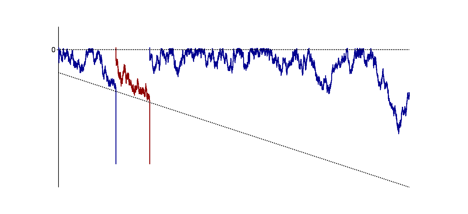
Figure 1: Sample trajectory of the diffusion $q^{\beta}_{\mu}$.

Roughly, the diffusion $q^{+}_{\mu}$ behaves as follows after each explosion time. First, it quickly goes down to values around $0$. Then, it spends some time between the line $t\mapsto c_{\mu}(t)$ and $0$, where it behaves as a reflected (downwards) Brownian motion with drift $a/4$. If it reaches the line $t\mapsto c_{\mu}(t)$ in a finite time then it quickly explodes to $-\infty$ after this hitting time.

The behaviour of the diffusion $q^{-}_{\mu}$ is similar except that in the interval $[c_{\mu}(t),0]$, it behaves as a reflected (downwards) Brownian motion with drift $-(a+1)/4$. Therefore, it almost surely hits $c_{\mu}(t)$ when $a>0$.

There are two types of explosions for $q^{\beta}_{\mu}$: either $q^{\beta}_{\mu}$ explodes at a time $\xi^{+}$ such that $q^{\beta}_{\mu}(\xi^{+})=q^{+}_{\mu}(\xi^{+})$, which corresponds to the (rescaled) hitting times of $0$ by the initial diffusion $p^{\beta}_{\Lambda^{\beta}}$, or $q^{\beta}_{\mu}$ explodes at time $\xi^{-}$ such that $q^{\beta}_{\mu}(\xi^{-})=q^{-}_{\mu}(\xi^{-})$, in which case we get the (rescaled) explosion times of the initial diffusion $p^{\beta}_{\Lambda^{\beta}}$.

In the following, we denote by $\xi^{+}_{\beta}(0)<\xi^{-}_{\beta}(0)<\xi^{+}_{\beta}(1)<\xi^{-}_{\beta}(1)<\ldots$ the explosion times of the diffusion $q_{\mu}^{\beta}$ and by

$$\nu^{\beta}_{\mu}:=\sum_{i\geqslant 0}\delta_{\xi^{-}_{\beta}(i)}\,$$ (8)

the measure corresponding to the (rescaled) explosions of $p^{\beta}_{\Lambda^{\beta}}$.

We will prove that, for a well-chosen topology, the trajectory of the diffusion $q^{\beta}_{\mu}$ converges in law, when $\beta$ tends to $0$, towards a non-trivial limit $r_{\mu}$, that we describe in the following paragraph.

3.3 Description of the limiting point process

Let us now define $r_{\mu}$, the limiting diffusion of $q^{\beta}_{\mu}$, which will characterize the limiting point process from Theorem 2.1. Its definition involves Brownian motions with drift reflected downwards at $0$. By definition, a Brownian motion with drift $\alpha$ reflected downwards at $0$ is a diffusion Markov process with infinitesimal operator $G\;:\;f\in\mathcal{D}\mapsto\frac{1}{2}f^{\prime\prime}+\alpha f^{\prime}$ acting on the domain

$$\mathcal{D}:=\Big{\{}f\in C_{b}[0,\infty[,Gf\in C_{b}\big{(}[0,\infty[\big{)},\;\lim_{x\downarrow 0}f^{\prime}(x)=0\Big{\}}\,,$$

where $C_{b}\big{(}[0,\infty[\big{)}$ denotes the continuous and bounded functions on $[0,\infty[$. Using the Skorohod problem, we can write this diffusion as

$$B(t)+\alpha t-\sup_{s\leqslant t}\big{(}B(s)+\alpha s\big{)}\vee 0\,,$$

where $B$ is a Brownian motion starting at $0$ or any negative point.

To define the limiting diffusion $r_{\mu}$, we use the same Brownian motion $W$ as in the diffusions $q_{\mu}^{+}$ and $q_{\mu}^{-}$ from (5) and (6).

Definition 3.1 (Limiting diffusion)

The limiting diffusion $r_{\mu}$ is defined as follows:

• It starts at $0$ at time $0$: $r_{\mu}(0)=0$.

• It then follows a Brownian motion with drift $a/4$ reflected downwards at $0$ (built from $W$)

  $$r^{+}:=W(t)+at/4-\sup_{s\leqslant t}\big{(}W(s)+as/4\big{)}\vee 0\,$$ (9)

  until its first hitting time of the critical line $c_{\mu}(t)$ from (7).

• If it reaches $t\mapsto c_{\mu}(t)$ in a finite time, it immediately restarts at $0$ at this time, then follows a reflected downwards at $0$ Brownian motion with another drift $-(a+1)/4$ (also built from $W$)

  $$r^{-}:=W(t)-(a+1)t/4-\sup_{s\leqslant t}\big{(}W(s)-(a+1)s/4\big{)}\vee 0\$$ (10)

  until its first hitting time of the critical line $c_{\mu}(t)$ from (7).

And so on, $r_{\mu}$ alternating between $r^{+}$ and $r^{-}$ each time it hits $t\mapsto c_{\mu}(t)$ and restarts at $0$. Note that the probability that $r^{+}$ reaches the critical line decreases with time. On the other hand, since $a>0$, $r^{-}$ almost surely hits the critical line in a finite time.

Let $\xi^{+}_{0}(0)<\xi^{-}_{0}(0)<\xi^{+}_{0}(1)<\xi^{-}_{0}(1)<\ldots$ be the hitting times of the critical line $c_{\mu}$ by the diffusion $r_{\mu}$, where we omit to display the dependency on $\mu$ for lighter notations. We define the random measure associated to the point process $\big{(}\xi^{-}_{0}(k),\;k\geqslant 0\big{)}$:

$$\nu^{0}_{\mu}:=\sum_{i\geqslant 0}\delta_{\xi^{-}_{0}(i)}\,.$$ (11)

We then use the coupled random measures $\big{(}\nu^{0}_{\mu},\;\mu>0\big{)}$ to define a discrete point process on $\mathbb{R}_{+}$. Since $\mu\in\mathbb{R}_{+}\mapsto\nu_{\mu}(\mathbb{R}_{+})$ decreases from $\infty$ to $0$ almost surely, it is easy to prove the following proposition:

Proposition 3.2 (Limiting point process)

There is a random variable $M_{0}$ valued in the Borel sets of $]0,\infty[$, such that, for all fixed $\mu_{1}<\ldots<\mu_{k}$,

$$M_{0}[\mu_{i},\infty[=\nu^{0}_{\mu_{i}}(\mathbb{R}_{+})\,.$$

Almost surely, the measure $M_{0}$ is unique, discrete, bounded from above and has an accumulation point at $0$.

3.4 Strategy of the proof of Theorem 2.1

We can now state the desired convergence results towards the limiting measures which we need to prove Theorem 2.1.

Proposition 3.3 (Convergence of the explosion times of $p^{\beta}_{\Lambda^{\beta}}$)

When $\beta$ tends to $0$, the measure $\nu^{\beta}_{\mu}$ (as in (8)) converges to the measure $\nu^{0}_{\mu}$ (as in (11)), for the topology of weak convergence.

It is immediate to extend this proposition for the joint law of $\nu^{\beta}_{\mu_{i}}$ when $\mu_{1},\ldots,\mu_{k}$ are fixed positive numbers. It directly implies the following result on the finite dimensional laws of the point process $\big{\{}\mu^{\beta}(i),\;i\geqslant 0\big{\}}$, with $\mu^{\beta}(i)$ as in (2). Let us denote by $M_{\beta}$ the measure associated to this point process, i.e. $M_{\beta}:=\sum_{i\geqslant 0}\delta_{\mu^{\beta}(i)}$.

Proposition 3.4 (Convergence of the finite-marginals of the eigenvalue process)

Fix $\mu_{1}<\ldots<\mu_{k}$. When $\beta\to 0$, the random vector $\big{(}M_{\beta}[\mu_{1},\infty[,\ldots,M_{\beta}[\mu_{k},\infty[\big{)}$ converges in law to the random vector $\big{(}M_{0}[\mu_{1},\infty[,\ldots,M_{0}[\mu_{k},\infty[\big{)}$.

Using a similar reasoning as in [3, Proof of Theorem $1$], we consider the space of measures on $]0,\infty[$ with the topology that makes continuous the maps $m\mapsto\langle f,m\rangle$ for any continuous and bounded function $f$ with support bounded to the left. In other words, this is the vague topology towards $0$ and the weak topology towards $\infty$. It allows to control the decreasing sequence of atom locations of $M_{\beta}$ from its first point.

Proposition 3.4 shows that the family of measures $(M_{\beta})_{\beta>0}$ is tight (and therefore relatively compact by Prokhorov’s theorem): indeed, the above convergence provides the required control on the mass given by $M_{\beta}$ to $[\mu,\infty[$ for any given $\mu>0$. Besides, this convergence uniquely identifies the finite-marginals of any limiting point. We thus deduce from Proposition 3.4 the convergence of the left-vague/right-weak topology of the eigenvalues point process stated in Theorem 2.1.

To conclude the proof of Theorem 2.1, we devote the rest of the paper to the proof of Proposition 3.3, also using the unique identification of the finite-marginals and the tightness of the family of measures. In Section 4, we control the first explosion time of the diffusion $q_{\mu}^{\beta}$ in (15) and deduce the weak convergence of its $k$ first explosions times. Then, in Section 5, we show the tightness of the family of measures $(\nu^{\beta}_{\mu})_{\beta>0}$.

Unless specified otherwise, the limits and $o$ now pertain to the asymptotics $\beta\rightarrow 0$. For lighter notations, we also omit the dependency on $\beta$ of our variables.

3.5 Useful concepts and results

We will use the following estimates for any Brownian motion $B$:

$$\forall x\geqslant 0,\ \mathbb{P}\Big{(}\underset{s\in[0,1]}{\sup}B(s)>x\Big{)}\leqslant\mathbb{P}\Big{(}\underset{s\in[0,1]}{\sup}\big{\lvert}B(s)\big{\rvert}>x\Big{)}\leqslant 4e^{-x^{2}/2},$$ (12)

$$\forall x\geqslant 0,\ \mathbb{P}\Big{(}\underset{s\in[0,1]}{\sup}B(s)>x\Big{)}=\mathbb{P}\Big{(}\big{\lvert}B(1)\big{\rvert}>x\Big{)}\geqslant 1-\sqrt{\frac{2}{\pi}}x.$$ (13)

Consider a diffusion $y$ started from $0$ and the same diffusion $\overline{y}$ reflected downwards at the origin:

$$\overline{y}(t)=y(t)-\ \underset{s\leqslant t}{\sup}\ y(s).$$

For all $\delta>0$, $\big{\{}\overline{y}(t)<-\delta\big{\}}=\big{\{}\exists s<t,\ y(t)-y(s)<-\delta\big{\}}$, therefore:

$$\underset{s\in[0,t]}{\sup}\big{\lvert}y(s)\big{\rvert}<\delta/2\Rightarrow\underset{s\in[0,t]}{\inf}\overline{y}(s)>-\delta.$$ (14)

4 Control of the explosion times

In this section, we fix $\mu>0$. Recall the definition of the critical line $c=c_{\mu}$ in (7). Consider the first two explosion times $\xi^{+}:=\xi_{\beta}^{+}(0)$ and $\xi^{-}:=\xi_{\beta}^{-}(0)$ of the diffusion $q_{\mu}^{\beta}$. Until the first explosion time $\xi^{+}$, by definition $q_{\mu}^{\beta}(0)=\infty$ and $q_{\mu}^{\beta}(t)=q^{+}(t)$ follows the SDE (5).

Set $\delta=\beta^{1/8}$ and introduce the first hitting times by the diffusion $q^{+}$:

$$\tau_{0}:=\inf\big{\{}t\geqslant 0,\;q^{+}(t)\leqslant 0\big{\}}\text{ and }\tau_{c}:=\inf\big{\{}t\geqslant 0,\;q^{+}(t)\leqslant c(t)+\delta\big{\}}.$$

We decompose the trajectory of $q^{+}$ into three parts. First, it reaches the axis $x=0$ in a short time (descent from $\infty$). Then, it spends a time of order $O(1)$ in the region $[c(t)+\delta,0]$ and behaves like $r^{+}$, the reflected Brownian motion with drift $a/4$ from (9). Finally, if it approaches the critical line $t\mapsto c(t)$ closer than $\delta$, then it explodes with high probability within a short time (explosion to $-\infty$).

Recall the first hitting times $\xi_{0}^{+}(0)<\xi_{0}^{-}(0)$ of the critical line $c$ by the diffusion $r_{\mu}$ from Definition 3.1.

Proposition 4.1 (Limit behavior of the diffusions $q^{+}$ and $q^{-}$)

Set $T>0$, independent of $\beta$. There exist a deterministic function $\eta(\beta)\rightarrow 0$ and an event $\mathcal{E}_{0}$, $\mathbb{P}(\mathcal{E}_{0})\rightarrow 1$, on which, for $\beta$ small enough:

1. $\tau_{0}<\beta$,

2. $\underset{[\tau_{0},\tau_{c}\wedge T]}{\sup}\big{\lvert}q^{+}(t)-r^{+}(t)\big{\rvert}<\delta$,

3. $\tau_{c}<T\Rightarrow\lvert\xi^{+}-\tau_{c}\rvert<\eta$ and $\lvert\xi_{0}^{+}(0)-\tau_{c}\rvert<\eta$.

Properties (a), (b) and (c) also hold for the diffusions $q^{-}$ from (6) and $r^{-}$ from (10), with their corresponding hitting and explosion times. As a consequence, on the event $\mathcal{E}_{0}$, for $\beta$ small enough,

$$\xi^{-}<T\Rightarrow\big{\lvert}\xi^{-}-\xi_{0}^{-}(0)\big{\rvert}<2\eta.$$ (15)

The control (15) extends to any $\xi_{\beta}^{-}(k)$ and $\xi_{0}^{-}(k)$ for $k\in\mathbb{N}$ and ensures that, for any $T>0$, $\mathbb{P}(\xi_{\beta}^{-}(k)\leqslant T)\rightarrow\mathbb{P}(\xi_{0}^{-}(k)\leqslant T)$, thus identifying the measure $\nu_{\mu}^{0}$ as the unique possible limit for $\nu_{\mu}^{\beta}$.

The rest of this section is dedicated to the proof of Proposition 4.1. Recall that the diffusion $q^{-}$ differs from its counterpart $q^{+}$ only by its constant drift component $-(a+1)/4$ (instead of $+a/4$ for $q^{+}$), which makes $q^{-}$ decrease faster than $q^{+}$. We prove the results for the diffusion $q^{+}$, they extend to the diffusion $q^{-}$ with the same arguments.

We introduce the stationary diffusion $\overline{q}$ on $\mathbb{R}_{+}$, which we use to approximate $q^{+}$ in the region where the drift component $\exp\big{[}-\frac{1}{\beta}\big{(}q^{+}(t)-c(t)\big{)}\big{]}$ becomes negligible as $\beta$ tends to $0$:

$$\mathrm{d}\overline{q}(t)=\mathrm{d}W(t)+\frac{1}{4}\big{(}a-e^{\overline{q}(t)/\beta}\big{)}\mathrm{d}t.\\$$ (16)

4.1 Descent from $\infty$: proof of $(a)$

It suffices to prove property $(a)$ for the diffusion $\overline{q}$, which bounds the diffusion $q^{+}$ from above. Set the level $l_{1}:=\beta^{3/4}$, so that $\beta=o(l_{1})$. As $\beta$ tends to $0$, when the diffusion $\overline{q}$ is above the level $l_{1}$, the term of leading order in the right-hand side of (16) is $e^{\overline{q}(t)/\beta}$.

Consider the ordinary differential equation on $\mathbb{R}_{+}$:

$$\mathrm{d}y(t):=\frac{1}{4}(a-e^{y(t)/(2\beta)})\mathrm{d}t,\ y(0)=\infty,$$

which has for solution $y(t)=-2\beta\ln\big{(}\frac{1}{a}(1-e^{-at/(8\beta)})\big{)}$. The time $t_{1}$ at which $y$ reaches the level $l_{1}/2$ has the asymptotics

$$t_{1}=8\beta e^{-l_{1}/(4\beta)}+o(\beta e^{-l_{1}/(4\beta)}).$$

Introduce the diffusion $\overline{q}_{1}(t):=\overline{q}(t)-W(t)$. Its evolution writes:

$$\mathrm{d}\overline{q}_{1}(t)=\frac{1}{4}\Big{(}a-e^{\big{(}\overline{q}_{1}(t)+W(t)\big{)}/\beta}\Big{)}\mathrm{d}t.$$

Let $\mathcal{E}^{\prime}_{1}:=\big{\{}\underset{[0,t_{1}]}{\sup}\big{\lvert}W(t)\big{\rvert}\leqslant\beta^{2}\big{\}}$. By the Brownian tail bound (12), $\mathbb{P}(\mathcal{E}^{\prime}_{1})\longrightarrow 1$. On the event $\mathcal{E}^{\prime}_{1}$ and while $\overline{q}_{1}(t)\geqslant l_{1}/2$, we have

$$\left|\frac{W(t)}{\overline{q}_{1}(t)}\right|\leqslant\frac{\beta^{2}}{l_{1}/2}\,,\ \text{ i.e }\ \left|\frac{W(t)}{\overline{q}_{1}(t)}\right|\leqslant 2\beta^{5/4}$$

and thus $\overline{q}_{1}(t)+W(t)\geqslant\overline{q}_{1}(t)/2$ for $\beta$ small enough.

Therefore the diffusion $\overline{q}_{1}$ is bounded from above by $y$ for $\beta$ small enough and hits the level $l_{1}/2$ before time $t_{1}$. Since $\big{\lvert}\overline{q}_{1}(t)-\overline{q}(t)\big{\rvert}\leqslant\beta^{2}$ before time $t_{1}$, for $\beta$ small enough, the diffusion $\overline{q}$ hits the level $l_{1}$ before time $t_{1}$ .

After the level $l_{1}$ is reached, we use the Brownian motion $W(t_{1}+\cdot)-W(t_{1})$ to reach $x=0$ in a short additional time. Set the event

$$\mathcal{E}^{{}^{\prime\prime}}_{1}:=\Big{\{}\underset{[0,\beta/2]}{\inf}\Big{\{}W(t_{1}+t)-W(t_{1})+\frac{a}{4}t\Big{\}}<-l_{1}\Big{\}},$$

on which $\tau_{0}<t_{1}+\beta/2$. Since $\mathbb{P}\big{(}\mathcal{E}^{{}^{\prime\prime}}_{1}\big{)}\geqslant\mathbb{P}\Big{(}\underset{[0,\beta/2]}{\inf}W(t_{1}+t)-W(t)<-l_{1}-\frac{a}{8}\beta\Big{)}$, the lower bound (13) and the asymptotics $\beta=o(l_{1})$ and $l_{1}=o(\sqrt{\beta})$ imply that $\mathbb{P}\big{(}\mathcal{E}^{{}^{\prime\prime}}_{1}\big{)}\longrightarrow 1$, thus proving the property $(a)$ on the event $\mathcal{E}_{1}=\mathcal{E}^{\prime}_{1}\cap\mathcal{E}^{{}^{\prime\prime}}_{1}$.

4.2 Convergence to $r^{+}$: proof of $(b)$

The bound (12) shows that the probability of the following event tends to $1$ as $\beta$ tends to $0$:

$$\mathcal{E}^{\prime}_{2}=\big{\{}\underset{t\in[0,\beta]}{\sup}\lvert W(t)\rvert\leqslant\beta^{1/4}\big{\}}.$$

Recall that $\delta=\beta^{1/8}$ so $\beta^{1/4}=o(\delta)$, and note that the diffusion $r^{+}(\tau_{0}+t)-r^{+}(\tau_{0})$ is equal in law to the diffusion $r^{+}$ (as in (9)), by the strong Markov property. Thus, to prove property $(b)$, it suffices to show that, with overwhelming probability as $\beta$ tends to $0$, for $\beta$ small enough,

$$\underset{[0,\tau^{\prime}_{c}\wedge T]}{\sup}\big{\lvert}q_{0}^{+}(t)-r^{+}(t)\big{\rvert}<\delta/2,$$ (17)

where $q_{0}^{+}$ denotes the diffusion $q^{+}$ started from $x=0$ at time $t=0$ and $\tau^{\prime}_{c}$ its first hitting time of $c(t)+\delta$. We write $\overline{q}_{0}$ the stationary diffusion $\overline{q}$ from (16) started from $x=0$ at time $t=0$. For $t\in[0,\tau^{\prime}_{c}\wedge T]$, $q_{0}^{+}(t)\geqslant c(t)+\delta$, so we have the bounds:

$$\forall t\in[0,\tau^{\prime}_{c}\wedge T],\ \overline{q}_{0}(t)-e^{-\delta/\beta}T\leqslant q_{0}^{+}(t)\leqslant\overline{q}_{0}(t).$$

Since $e^{-\delta/\beta}=o\big{(}\delta\big{)}$, to prove property (17), it is enough to show that, on an event $\mathcal{E}^{\prime}_{2}$ of probability going to $1$ as $\beta$ tends to $0$, for $\beta$ small enough,

$$\underset{[0,\tau^{\prime}_{c}\wedge T]}{\sup}\big{\lvert}\overline{q}_{0}(t)-r^{+}(t)\big{\rvert}<\delta/4.$$ (18)

To that end, we bound the diffusion $\overline{q}_{0}(t)$ from below and above by two reflected diffusions $r^{+}_{1}$ and $r^{+}_{2}$ that converge to $r^{+}$ as $\beta$ tends to $0$.

We set the level $l_{2}:=\beta^{1/6}$, so that $l_{2}=o(\delta)\text{ and }\delta=o(\sqrt{l_{2}})$.

4.2.1 Lower bound

We set the level $l_{2}:=\beta^{1/6}$. Let $r_{1}^{+}$ be the following diffusion, reflected downwards at the barrier $-l_{2}$:

$$r_{1}^{+}(t):=-l_{2}+W(t)+at/4-e^{-\frac{l_{2}}{\beta}}T/4-\sup_{s\leqslant t}\big{(}W(s)+as/4-e^{-\frac{l_{2}}{\beta}}T/4\big{)}\vee 0.$$

Since the element of drift $-e^{\overline{q}_{0}(t)/\beta}$ decreases when $\overline{q}_{0}(t)$ goes through $\big{]}-\infty,-l_{2}\big{]}$, we have the lower bound:

$$\forall t\in[0,\tau^{\prime}_{c}\wedge T],\ \overline{q}_{0}(t)\geqslant r_{1}^{+}(t).$$ (19)

It is straightforward that

$$\forall t\in[0,\tau^{\prime}_{c}\wedge T],\ r^{+}(t)-e^{-\frac{l_{2}}{\beta}}T/4-l_{2}\leqslant r_{1}^{+}(t)\leqslant r^{+}(t)-l_{2}.$$

Since $e^{-\frac{l_{2}}{\beta}}=o(l_{2})$, for $\beta$ small enough,

$$\underset{[0,\tau^{\prime}_{c}\wedge T]}{\sup}\big{\lvert}r^{+}(t)-r_{1}^{+}(t)\big{\rvert}<2l_{2}.$$

4.2.2 Upper bound

We wish to bound the diffusion $\overline{q}_{0}(t)$ from above by the diffusion $r^{+}(t)+l_{2}$. To prove that this upper bound holds with high probability as $\beta$ tends to $0$, we use the following result, that shows how unlikely it becomes for the diffusion $\overline{q}_{0}(t)$ to hit the level $l_{2}$ before any negative level.

Lemma 4.2 (Levels hitting times for the diffusion $\overline{q}_{0}(t)$)

For any $\gamma<0$,

$$\mathbb{P}\Big{(}\inf\big{\{}t\geqslant 0,\ \overline{q}_{0}(t)=l_{2}\big{\}}<\inf\big{\{}t\geqslant 0,\ \overline{q}_{0}(t)=\gamma\big{\}}\Big{)}\longrightarrow 0.$$

Lemma 4.2 is proved in the Appendix using standard tools of diffusion analysis.

The choice of level $\gamma=-c(T)$ in Lemma 4.2 provides the existence of an event $\mathcal{E}^{\prime}_{2}$ of probability going to $1$ as $\beta$ tends to $0$ on which the diffusion $\overline{q}_{0}(t)$ hits the barrier $c(t)$ before the level $l_{2}$, and thus:

$$\forall t\ \in[0,\tau^{\prime}_{c}\wedge T],\ \overline{q}_{0}(t)\leqslant r^{+}(t)+l_{2}.$$ (20)

4.2.3 Conclusion

Gathering (19) and (20), we get that, on $\mathcal{E}^{\prime}_{2}$, for $\beta$ small enough,

$$\forall t\ \in[0,\tau^{\prime}_{c}\wedge T],r_{1}^{+}(t)\leqslant\overline{q}_{0}(t)\leqslant r^{+}(t)+l_{2},$$

which implies $\underset{[0,\tau^{\prime}_{c}\wedge T]}{\sup}\big{\lvert}\overline{q}_{0}(t)-r^{+}(t)\big{\rvert}<2l_{2}$. This in turn implies (18) and thus proves property $(b)$.

4.3 Explosion to $-\infty$: proof of $(c)$

We denote by $q_{+\delta}^{+}$ (resp. $q_{-\delta}^{+}$) the diffusion $q^{+}$ started at time $t=0$ from position $-\mu+\delta$ (resp. $-\mu-\delta$). We introduce the first hitting time $\tau_{\delta}$ of the level $c(t)-\delta$ by the diffusion $q_{+\delta}^{+}$, and the explosion time $\tau_{-\infty}$ of the diffusion $q_{-\delta}^{+}$ to $-\infty$.

Recall that $l_{2}=\beta^{1/6}$. To prove property $(c)$, we choose $\eta:=2l_{2}$ and show that there exists an event of probability going to $1$ as $\beta$ tends to $0$ on which, for $\beta$ small enough, $\tau_{\delta}<\eta/2$ and $\tau_{-\infty}<\eta/2$.

4.3.1 Control of $\tau_{\delta}$

Recall that $\delta=\beta^{1/8}$, so that $l_{2}=o(\delta)$ and $\delta=o(\sqrt{l_{2}})$.

We use the variations of the Brownian motion $W$ to cross the critical line $c(t)$. The upper bound $q_{\delta}^{+}(t)\leqslant-\mu+\delta+W(t)+\frac{a}{4}t$ implies that $\tau_{\delta}<l_{2}$ on the event

$$\mathcal{E}_{3}:=\bigg{\{}\underset{[0,l_{2}]}{\inf}\Big{\{}W(s)+\frac{a}{4}s+\frac{1}{4}s+2\delta\Big{\}}<0\bigg{\}},$$

and the Brownian tail bound from (13) shows that $\mathbb{P}\big{(}\mathcal{E}_{3}\big{)}\rightarrow 1$.

Note that the inclusion of events $\mathcal{E}^{\prime}_{3}\subset\Big{\{}\inf\big{\{}t\geqslant 0,\ r^{+}(t)+t/4\leqslant-2\delta\big{\}}<l_{2}\Big{\}}$ ensures that, on a subevent of $\mathcal{E}_{2}$ (where $\lvert q^{+}(\tau_{c})-r^{+}(\tau_{c})\rvert<\delta$ if $\tau_{c}<\infty$) of probability going to $\mathbb{P}(\mathcal{E}_{2})$ as $\beta$ tends to $0$, the diffusion $r^{+}$ hits the critical line $c(t)$ while the diffusion $q^{+}$ crosses this line, between times $\tau_{c}$ and $\tau_{c}+\eta$.

4.3.2 Control of $\tau_{-\infty}$

On each Brownian trajectory, the diffusion $q_{-\delta}^{+}$ is bounded from above by the diffusion $z$, with

$$\mathrm{d}z(t):=\mathrm{d}W(t)+\frac{1}{4}\big{(}a-e^{-\frac{1}{\beta}\big{(}t/4+\mu+z(t)\big{)}}\big{)}\mathrm{d}t,\ z(0)=-\mu-\delta.$$

Define the diffusion $z_{1}(t)=z(t)+\mu-W(t)-at/4$, with evolution

$$\mathrm{d}z_{1}(t):=-\frac{1}{4}e^{-\frac{1}{\beta}\big{(}z_{1}(t)+t/4+W(t)+at/4\big{)}}\mathrm{d}t,\ z_{1}(0)=-\delta.$$

Consider the event $\mathcal{E}_{3}^{{}^{\prime}}:=\big{\{}\underset{[0,\beta]}{\sup}\ \lvert W(t)\rvert\leqslant\delta/4\big{\}}$, with $\mathbb{P}\big{(}\mathcal{E}_{3}^{{}^{\prime}}\big{)}\rightarrow 1$.

On $\mathcal{E}_{3}^{{}^{\prime}}$, for $\beta$ small enough:

$$\forall t\leqslant\beta,\ W(t)+\frac{a+1}{4}t\leqslant\delta/2,$$

so the diffusion $z_{1}$ is bounded from above by the solution $z_{2}$ of the ordinary differential equation

$$\mathrm{d}z_{2}(t):=-\frac{1}{4}e^{-\frac{1}{\beta}\big{(}z_{2}(t)+\delta/2\big{)}}\mathrm{d}t,\ z_{2}(0):=-\delta$$

with solution

$$z_{2}(t)=-\delta/2+\beta\ln\big{(}e^{-\delta/(2\beta)}-\frac{t}{4\beta}\big{)},$$

which explodes to $-\infty$ in a time $4\beta e^{-\delta/(2\beta)}$, smaller than $\beta$ for $\beta$ small enough. This remains true for $z_{1}$ and thus for $z$, since $\lvert z_{1}-z\rvert\leqslant\mu+a\beta/4+\beta$ while $t\leqslant\beta$. Since $\beta=o(\eta)$, this proves the desired control on $\tau_{-\infty}$.

5 Tightness of the explosion times measures

In this section, we fix $\mu>0$. Recall the measure of the explosion times $\nu_{\mu}^{\beta}$ from (8) . We prove in this section that there are $\beta_{0}>0$ and $\alpha>0$, such that, for all $\epsilon>0$, there exist a finite time $T_{\epsilon}$ and a finite number of explosions $N_{\epsilon}$ so that:

$$\underset{\beta\leqslant\beta_{0}}{\inf}\mathbb{P}\bigg{(}\Big{\{}\nu_{\mu}^{\beta}\big{(}[0,\alpha T_{\epsilon}]\big{)}\leqslant N_{\epsilon}\Big{\}}\bigcap\Big{\{}\nu_{\mu}^{\beta}\big{(}[\alpha T_{\epsilon},\infty[\big{)}=0\Big{\}}\bigg{)}>1-\epsilon.$$ (21)

Introduce $\mathcal{L_{\mu}^{\beta}}$, the law of the random measure $\nu_{\mu}^{\beta}$. The bound (21) gives us the tightness condition:

$$\exists\beta_{0},\ \forall\epsilon>0,\ \exists K_{\epsilon}\text{ compact},\ \underset{\beta<\beta_{0}}{\sup}\ \mathcal{L_{\mu}^{\beta}}(K_{\epsilon})\geqslant 1-\epsilon.$$ (22)

Indeed, the set $\mathring{K}_{\epsilon}:=\big{\{}\mu\in\mathcal{P},\ \mu([0,\alpha T_{\epsilon}])\leqslant N_{\epsilon}\text{ and }\mu\big{(}[\alpha T_{\epsilon},\infty[\big{)}=0\big{\}}$, where $\mathcal{P}$ is the space of locally finite measures on $\mathbb{R}_{+}$, satisfies the following conditions:

$$\begin{split}\underset{\mu\in\mathring{K}_{\epsilon}}{\sup}\mu(\mathbb{R_{+}})<\infty,\\ \underset{t>0}{\inf}\ \underset{\mu\in\mathring{K}_{\epsilon}}{\sup}\mu\big{(}[t,\infty[\big{)}=0,\end{split}$$ (23)

where the second condition holds since, for any measure $\mu$ in $\mathring{K}_{\epsilon}$ and $t\geqslant\alpha T_{\epsilon},\ \mu\big{(}[t,\infty[\big{)}=0$. It thus fulfills the Kallenberg criterion for weak relative compactness (see [10]), and its compact closure $K_{\epsilon}$ verifies the tightness condition (22).

Prokhorov’s theorem gives us the relative compactness of the family $(\mathcal{L_{\mu}^{\beta}})_{\beta<\beta_{0}}$ in $\mathcal{M}^{1}(\mathcal{P})$, the set of probability measures on $\mathcal{P}$, and thus concludes the proof of Proposition 3.3.

The rest of this section is dedicated to the proof of (21). We first show a preliminary result that will be helpful to control the number of explosions. Recall that $\xi^{+}=\xi_{\beta}^{+}(0)$ is the first explosion time of the diffusion $q^{+}$ from (5), started from $\infty$ at time $0$.

Lemma 5.1 (Lower bound on the explosion time of $q^{+}$)

For $\beta$ small enough,

$$\forall t>0,\ \mathbb{P}\big{(}\xi^{+}>t\big{)}\geqslant 1-4e^{-\mu^{2}/(32t)}.$$

Proof 5.2

We fix a deterministic $\delta_{0}$ such that $0<\delta_{0}<\mu/4$. Recall the definition of the critical line $c_{\mu}$ in (7). When the diffusion $q^{+}$ is in the region between $-c_{\mu}(t)+\delta_{0}$ and $-\delta_{0}$, we have the lower bound, for $\beta$ small enough:

$$a-e^{q^{+}(t)/\beta}-e^{-\frac{1}{\beta}(\mu(t)+q^{+}(t))}\geqslant a-2e^{-\delta_{0}/\beta}\geqslant 0.$$ (24)

Introduce the diffusion $\widehat{q}$ on $\mathbb{R}_{+}$, defined as the Brownian motion $W(t)$ started from $-\delta_{0}$ at time $0$ and reflected downwards at $-\delta_{0}$: $\widehat{q}(t):=-\delta_{0}+W(t)-\sup_{s\leqslant t}\big{(}W(s)\big{)}\vee 0.$ The bound (24) shows that, for $\beta$ small enough, the diffusion $q^{+}$ is bounded from below by the diffusion $\widehat{q}$ on each Brownian trajectory, up until the first hitting time of $c_{\mu}(t)+\delta_{0}$ by $q^{+}$.

Set $t>0$ and introduce the event $\mathcal{E}:=\big{\{}\underset{s\in[0,t]}{\sup}\big{\lvert}W(s)\big{\rvert}<\mu/4\big{\}}$. By the Brownian tail bound (12), we have $\mathbb{P}(\mathcal{E})\geqslant 1-4e^{-\mu^{2}/(32t)}$. Besides, on the event $\mathcal{E}$, using (14),

$$\forall s\in[0,t],\ \widehat{q}(s)>-\delta_{0}-\mu/2.$$

This means that the diffusion $\widehat{q}$ stays above $-\mu$ until time $t$. Thus, for $\beta$ small enough so that (24) holds, on the event $\mathcal{E}$, we have $\xi^{+}>t$.

We now turn to the proof of (21). Fix $\epsilon>0$. We control the diffusion $q_{\mu}^{\beta}$ with two diffusions. The first diffusion $Q_{1}$ starts at time $T_{\epsilon}$ at position $-1$ and is reflected below the horizontal line $-1$ with drift $a/8$. The second diffusion $Q_{2}$ starts at time $2T$ at position $c_{\mu}(T_{\epsilon})$, has a drift $a/8$ as well and is also reflected below $-1$.

We can choose $T_{\epsilon}$ high enough such that the diffusions $Q_{1}$ and $Q_{2}$ do not hit $c_{\mu}(t)+1$ with probability greater than $1-\epsilon/10$. Indeed, the sublinearity of the Brownian motion $W(T_{\epsilon}+t)-W(T_{\epsilon})$ is such that

$$\exists\ T_{0},\forall t\geqslant T_{0},\lvert W(T_{\epsilon}+t)-W(T_{\epsilon})\rvert<t/16\text{ with probability greater than }1-\epsilon/40.$$ (25)

On the event where (25) holds, the diffusion $Q_{1}$ stays above $-1-t/8$ after time $T_{0}$, and thus above the critical line $c_{\mu}(t)$. We now choose $T_{\epsilon}$ high enough so that $\lvert W(T_{\epsilon}+t)-W(t)\rvert<c_{\mu}(T)/4$ with probability greater than $1-\epsilon/40$ until time $T_{0}$, thus $Q_{1}$ stays above $c_{\mu}(t)$ before time $T_{0}$ as well. Therefore, on an event of probability greater than $1-\epsilon/20$, the diffusion $Q_{1}$ never hits $c_{\mu}(t)$. Similar arguments can be used for the second diffusion $Q_{2}$.

The term $-(a+1)/4$ in the drift of the diffusion $q^{-}$ implies the existence of $\alpha>0$ such that, almost surely, when started before time $2T_{\epsilon}+1$, the diffusion $q^{-}$ explodes before time $\alpha T_{\epsilon}$.

If, at time $T_{\epsilon}$, the diffusion $q_{\mu}^{\beta}$ evolves as the diffusion $q^{-}$, then it almost surely explodes before time $\alpha T_{\epsilon}$, after which it evolves as $q^{+}$ and stays above $Q_{1}$ (for $\beta$ small enough such that $2e^{-1/\beta}<a/8$) and does not explode anymore.
If, at time $T_{\epsilon}$, the diffusion $q_{\mu}^{\beta}$ evolves as the diffusion $q^{+}$, then we distinguish between three cases:
First, if the diffusion $q_{\mu}^{\beta}$ hits $-1$ between times $T_{\epsilon}$ and $2T_{\epsilon}$, then $q_{\beta}$ stays above $Q_{1}$ and therefore does not explode.
Else, following the proof of property $(c)$ from Proposition 4.1 in Section 4, we can choose a deterministic level $\delta_{1}>0$ so that, if $q_{\mu}^{\beta}$ reaches $t\mapsto c_{\mu}(t)+\delta_{1}$ between time $T_{\epsilon}$ and $2T_{\epsilon}$, then it explodes before time $2T_{\epsilon}+1$ with probability greater than $1-\varepsilon/10$. After that, $q_{\mu}^{\beta}$ behaves as $q^{-}$ and almost surely explodes one last time before time $\alpha T_{\epsilon}$, as previously.
Finally, if the diffusion $q_{\mu}^{\beta}$ starts above $c_{\mu}(T_{\epsilon})+\delta_{1}$ at time $T_{\epsilon}$ and stays in the interval $[c_{\mu}(t)+\delta_{1},-1]$ for all $t\in[T_{\epsilon},2T_{\epsilon}]$, then it is bounded from below by a Brownian motion with a positive drift $a/8$, and therefore it will be above $c_{\mu}(T)$ at time $2T_{\epsilon}$ with probability greater than $1-\epsilon/10$. In this event, $q_{\mu}^{\beta}$ stays above the diffusion $Q_{2}$ after time $2T_{\epsilon}$ and thus does not explode.

Gathering the different cases, we thus obtain the existence of an event of probability greater than $1-\epsilon/2$ on which $q_{\mu}^{\beta}$ explodes at most once after time $T_{\epsilon}$ and does not explode after time $\alpha T_{\epsilon}$.

To conclude the proof of the tightness criterion (21), we apply Lemma 5.1 to get the existence of a finite $N_{\epsilon}$ and of an event of probability greater than $1-\epsilon/2$ on which the diffusion $q_{\mu}^{\beta}$ explodes at most $N_{\epsilon}-1$ times before time $T_{\epsilon}$.

6 Conclusion

We proved that, in the high temperatures limit $\beta\rightarrow 0$, the properly rescaled point process of the low-lying eigenvalues of the stochastic Bessel operator converges towards a simple point process on $\mathbb{R}_{+}$, described using coupled SDEs. This limiting point process keeps a repulsive factor and therefore differs from the Poisson point process found by Dumaz and Labbé [3] as the high temperatures limit of the Stochastic Airy operator. Our result opens research perspectives to understand the properties of this new point process.

Appendix: Proof of Lemma 4.2

Recall that $l_{1}=\beta^{3/4}$ and $l_{2}=\beta^{1/6}$. In this proof we denote by $q$ the diffusion $\overline{q}_{0}^{+}$. Set $\gamma<0$, $\tau:=\inf\big{\{}t\geqslant 0,\ q_{0}^{+}(t)=l_{2}\big{\}}$ and $\tau^{\prime}:=\inf\big{\{}t\geqslant 0,\ q_{0}^{+}(t)=\gamma\big{\}}$. Let $f_{\beta}(x):=\frac{1}{4}\big{(}a-\exp(x/\beta)\big{)}$. To compute the hitting times of $q$, introduce the scale functions $\mathfrak{s}_{\beta}$ and $\mathfrak{s}$:

$$\mathfrak{s}_{\beta}(x) :=\int_{-1}^{x}\exp\Big{(}-2\int_{0}^{u}f_{\beta}(v)\mathrm{d}v\Big{)}\mathrm{d}u,$$

$$\mathfrak{s}(x) :=\int_{-1}^{x}\exp\Big{(}-2\int_{0}^{u}\frac{a}{4}\mathrm{d}v\Big{)}\mathrm{d}u=\frac{2}{a}\big{(}e^{a/2}-e^{ax/2}\big{)}.$$

The following lemma explicits the asymptotic behavior of $\mathfrak{s}_{\beta}$.

Lemma 6.1 (Convergence of the scale functions)

For any $x_{0}<0$,

$$\mathfrak{s}^{\prime}_{\beta}\longrightarrow\mathfrak{s}^{\prime}\text{ and }\mathfrak{s}_{\beta}\longrightarrow\mathfrak{s}\text{ uniformly on }[x_{0},0].$$

Furthermore, $\mathfrak{s}_{\beta}\big{(}l_{2}\big{)}\longrightarrow\infty$.

Since $\mathfrak{s}_{\beta}\big{(}q(\cdot)\big{)}$ is a local martingale, $\mathfrak{s}_{\beta}\big{(}q(\cdot\wedge\tau(q)\wedge\tau^{\prime}(q)\big{)}$ is a martingale. By the stopping theorem, we get:

$$\mathbb{P}\big{(}\tau<\tau^{\prime}\big{)}=\frac{\mathfrak{s}_{\beta}(\gamma)-\mathfrak{s}_{\beta}\big{(}0\big{)}}{\mathfrak{s}_{\beta}(\gamma)-\mathfrak{s}_{\beta}\big{(}l_{2}\big{)}}.$$

Lemma 6.1 readily implies that this probability tends to $0$ as $\beta$ tends to $0$.

Proof 6.2 (Proof of Lemma 6.1)

We have, for all $x\leqslant 0$,

$$\bigg{\lvert}\int_{0}^{x}f_{\beta}(v)-\frac{a}{4}\mathrm{d}v\bigg{\rvert}\leqslant\int_{x}^{0}e^{v/\beta}\mathrm{d}v\leqslant\beta\longrightarrow 0,$$

which means that $\ln\mathfrak{s}^{\prime}_{\beta}$ converges uniformly to $\ln\mathfrak{s}^{\prime}$ on $]-\infty,0]$. Besides, the functions $\ln\mathfrak{s}^{\prime}_{\beta}$ and $\ln\mathfrak{s}^{\prime}$ are bounded on $[x_{0},0]$, and $x\mapsto e^{x}$ is uniformly continuous on $[x_{0},0]$ so $\mathfrak{s}^{\prime}_{\beta}$ converges uniformly to $\mathfrak{s}^{\prime}$ on $[x_{0},0]$. Therefore, $\mathfrak{s}_{\beta}$ converges uniformly to $\mathfrak{s}$ on $[x_{0},0]$.

Now turning to $\mathfrak{s}_{\beta}\big{(}l_{2}\big{)}$. We can compute explicitly:

$$\ln\mathfrak{s}_{\beta}^{{}^{\prime}}(x)=-2\int_{0}^{x}f_{\beta}(v)\mathrm{d}v=-2ax+2\int_{0}^{x}e^{v/\beta}\mathrm{d}v=-2ax+2\beta\big{(}e^{x/\beta}-1\big{)}.$$

A study of the variations of $\ln\mathfrak{s}^{\prime}_{\beta}$ shows that $\mathfrak{s}^{\prime}_{\beta}$ decreases before $\beta\ln(2a)$ and increases afterwards. For $\beta$ small enough, $\ln\mathfrak{s}^{\prime}_{\beta}(l_{1})\geqslant\beta e^{l_{1}/\beta}$, which tends to $\infty$ as $\beta$ tends to $0$, and $\mathfrak{s}^{\prime}_{\beta}$ increases on $\big{[}l_{1},l_{2}\big{]}$, so that:

$$\mathfrak{s}_{\beta}\big{(}l_{2}\big{)}\geqslant\int_{l_{1}}^{l_{2}}\mathfrak{s}^{\prime}_{\beta}(v)\mathrm{d}v\geqslant\big{(}l_{2}-l_{1}\big{)}\mathfrak{s}^{\prime}_{\beta}(l_{1}),$$

therefore $\mathfrak{s}_{\beta}\big{(}l_{2}\big{)}\longrightarrow\infty$.

I wish to thank Laure Dumaz for her precious help throughout this research project.

This research paper presents results found during my PhD thesis [11], funded with a research grant from the SDOSE Doctoral School and PSL University.

There were no competing interests to declare which arose during the preparation or publication process of this article.

References

- [1] Bourgade, P., Erdős, L. and Yau, H. T. (2012). Bulk universality of general -ensembles with non-convex potential. J. Math. Phys. 53, 095221.
- [2] Bourgade, P., Erdős, L. and Yau, H. T. (2014). Universality of general -ensembles. Duke Math. J. 163, 1127 – 1190.
- [3] Dumaz, L. and Labbé, C. (2022). The stochastic airy operator at large temperature. The Annals of Applied Probability 32, 4481 – 4534.
- [4] Dumaz, L., Li, Y. and Valkó, B. (2021). Operator level hard-to-soft transition for -ensembles. Electron. J. Probab. 26, 28.
- [5] Dumitriu, I. and Edelman, A. (2002). Matrix models for beta ensembles. J. Math. Phys. 43, 5830–5847.
- [6] Dumitriu, I. and Edelman, A. (2006). Global spectrum fluctuations for the -hermite and -laguerre ensembles via matrix models. J. Math. Phys. 47, 063302.
- [7] Duy, T. K. (2018). On spectral measures of random Jacobi matrices. Osaka J. Math. 55, 595–617.
- [8] Erdős, L. and Yau, H. T. (2015). Gap universality of generalized Wigner and -ensembles. J. Eur. Math. Soc. 17, 1927–2036.
- [9] Halperin, B. I. (1965). Green’s functions for a particle in a one-dimensional random potential. Phys. Rev. 139, A104–A117.
- [10] Kallenberg, O. (2017). Random Measures, Theory and Applications vol. 77.
- [11] Magaldi, H. (2022). Beta-ensembles and their high-temperature limit. PhD thesis. Université PSL.
- [12] Ramírez, J. and Rider, B. (2009). Diffusion at the random matrix hard edge. Commun. Math. Phys. 288, 887–906.
- [13] Ramírez, J. A., Rider, B. and Virág, B. (2011). Beta ensembles, stochastic Airy spectrum, and a diffusion. J. Am. Math. Soc. 24, 919–944.
- [14] Shcherbina, M. (2011). Orthogonal and symplectic matrix models: Universality and other properties. Commun. Math. Phys. 307, 761–790.
- [15] Silverstein, J. W. (1985). The smallest eigenvalue of a large dimensional Wishart matrix. Ann. Probab. 13, 1364–1368.
- [16] Sosoe, P. and Wong, P. (2012). Local semicircle law in the bulk for gaussian -ensemble. J. of Statist. Phys. 148, 204–232.
- [17] Valkò, B. and Virág, B. (2009). Continuum limits of random matrices and the brownian carousel. Inventiones mathematicae 177, 463–508.
- [18] Wong, P. (2012). Local semicircle law at the spectral edge for gaussian -ensembles. Commun. Math. Phys. 312, 251–263.