Long-time analysis of a pair of on-lattice and continuous run-and-tumble particles with jamming interactions

Abstract

Run-and-Tumble Particles (RTPs) are a key model of active matter. They are characterized by alternating phases of linear travel and random direction reshuffling. By this dynamic behavior, they break time reversibility and energy conservation at the microscopic level. It leads to complex out-of-equilibrium phenomena such as collective motion, pattern formation, and motility-induced phase separation (MIPS). In this work, we study two fundamental dynamical models of a pair of RTPs with jamming interactions and provide a rigorous link between their discrete- and continuous-space descriptions. We demonstrate that as the lattice spacing vanishes, the discrete models converge to a continuous RTP model on the torus, described by a Piecewise Deterministic Markov Process (PDMP). This establishes that the invariant measures of the discrete models converge to that of the continuous model, which reveals finite mass at jamming configurations and exponential decay away from them. This indicates effective attraction, which is consistent with MIPS. Furthermore, we quantitatively explore the convergence towards the invariant measure. Such convergence study is critical for understanding and characterizing how MIPS emerges over time. Because RTP systems are non-reversible, usual methods may fail or are limited to qualitative results. Instead, we adopt a coupling approach to obtain more accurate, non-asymptotic bounds on mixing times. The findings thus provide deeper theoretical insights into the mixing times of these RTP systems, revealing the presence of both persistent and diffusive regimes.

Keywords: run-and-tumble particles, piecewise deterministic Markov processes, jamming, mixing time.

1 Introduction, models and main results

1.1 Introduction

Run-and-tumble particles (RTPs), which randomly switch between phases of linear motion (runs) through localized chaotic motion (tumbles) resulting in reorientation, are a prime example of active matter [Ram10]. Their self-propulsion breaks time reversibility and energy conservation at the microscopic scale, two fundamental properties of equilibrium systems. This leads to rich out-of-equilibrium behavior such as collective motion [VZ12], pattern formation [BB95] and motility induced phase separation (MIPS) [CT15]. In particular, accumulation at obstacles and MIPS both result in spatially inhomogeneous particle distributions, that deviate from the homogeneous passive particle ones. Thus they cannot a priori be framed into the equilibrium description based on an already known stationary distribution and their dynamics be summarized into a reversible random walk. Coarse-grained analytical approaches allowed to retrieve some observed mesoscopic behaviors, but are unfitted to trace back an observed behavior to a particular microscopic origin. More generally, there is still no systematic method for deriving directly from the microscopic details the exact form of the stationary distribution.

Some recent results were obtained for particular on-lattice models, consisting of two RTPs interacting through jamming [SEB16, SEB17]. The continuous-space invariant measure, formally obtained by making the lattice spacing go to zero, displays increased mass at jamming configurations. This increased mass takes the form of Diracs and, in the case of non-zero tumble duration [SEB17], exponentials, indicating effective attraction in line with MIPS. The same discretization scheme is revisited for models with collision induced recoil [MEB22, MEB23], leading to either effective attraction or repulsion depending on model parameters. A more direct approach based on piecewise deterministic Markov processes (PDMP) [Dav93] was introduced in [HGM23]. This allows to work directly with a continuous-space process, greatly simplifies computations and makes boundary conditions transparent. Indeed, in continuous space, jamming interactions between particles result in boundary conditions in the state space. Their thorough understanding is necessary in order to compute the invariant measure. Consequently, this PDMP approach enabled the computation of the explicit invariant measure of the two-RTP system with general tumbling and jamming behavior, revealing the existence of two universality classes distinguished by either a detailed or global probability flow preservation. While the invariant measures obtained with the PDMP approach in [HGM23] recover the continuous limit of the discrete processes in [SEB16, SEB17], the proof of such convergence, as the lattice spacing decreases, is still missing.

The computation of the invariant measures naturally leads to the question of the speed of convergence towards it. In the context of RTPs, this is linked to the time it takes for MIPS to emerge from an arbitrary configuration. Indeed, while the invariant measure of Markov processes determines their behavior at time scales of the order of their mixing time, it becomes irrelevant at smaller time scales. The most commonly used approach is spectral decomposition: the distance to the invariant measure decays exponentially, with an asymptotic rate determined by the second eigenvalue of the generator. The full spectral decomposition of two on-lattice RTPs on the 1D torus with jamming is computed in [MBE19], revealing eigenvalue crossings and a non-analytic spectral gap. In continuous space with added thermal noise [DDK20], the generator is a differential operator so the eigenvalue problem takes the form of an ODE. The full spectrum is again computed and the spectral gap is found to reduce to the spectral gap of the velocity dynamics as the length of the 1D torus goes to zero. This occurs because the time it takes to explore position space goes to zero while the time to explore velocity space remains constant. In [AG19], the eigenvalues are obtained as the poles of the Laplace transform in time of the position distribution and the same reduction phenomenon is observed. Unfortunately, when the generator is an unbounded operator, the set of eigenvalues can be a proper subset of the spectrum, complicating the computation of the spectral gap. Furthermore, because RTP systems are non-reversible, there is an uncontrolled prefactor to the exponential decay and the convergence results are only true in the asymptotic regime, leaving open the question in the non-asymptotic case.

In this work, we address these different convergence questions. The first result of this paper is that the continuous-space limit, where the lattice spacing tends to zero, of the Markov jump processes in [SEB16, SEB17] is a variant of the PDMP in [HGM23], rigorously linking the two models. The convergence is made quantitative by relying on a coupling strategy rather than the usual generator approach [EK86]. A uniformity result on the mixing times of the discrete-space processes is then used to prove that the on-lattice invariant measures converge to the continuous invariant measure for the Wasserstein distance, thus giving further theoretical underpinning to [SEB16, SEB17]. Secondly, regarding the long-time behavior, we adopt the coupling approach [FGM12] to obtain sharp non-asymptotic bounds. An order preservation argument, in the general spirit of [LMT96], reduces the coupling approach to hitting time computations and provides quantitative upper bounds on the mixing time. Matching lower bounds are established by identifying obstacles to mixing, which are then made quantitative by concentration inequalities. This shows that the bounds are optimal and fully capture the dependence of the mixing time on model parameters, incidentally revealing the existence of a persistent and diffusive regime similar to [DDK20, AG19].

In the remainder of this section, the discrete models from [SEB16, SEB17], as well as their continuous-space limit, are introduced and the main results are presented. The section ends with a plan of the paper.

1.2 Models and main results

1.2.1 Discrete process

All processes considered in this paper aim to describe the collective ballistic motion of a pairs of RTPs, that jam when they collide. We define the Markov jump process introduced in [SEB16, SEB17]. The goal is to show that this discrete model converges in law to particular instances of the general continuous-space stochastic process considered in [HGM23].

The discrete process of interest corresponds to the setting of two RTPs on a periodic one-dimensional lattice of $L+1$ sites, as illustrated in Fig. 1. Each particle is endowed with a velocity and an independent Poisson clock with rate $\gamma$. When their clock rings, the particles jump to the neighboring position in the direction of their velocity except if that position is occupied by the other particle. The particles thus display the persistent motion characteristic of RTPs as well as jamming interactions.

Figure 1: Sequence of random position jumps and velocity flips

In [SEB16], the tumbles are approximated by instantaneous reorientations and the velocities are independent Markov jump processes taking the values $1$ and $-1$ and following the transition rates of figure 2(a). In [SEB17], the tumbles have a finite nonzero duration so that the velocities can take the additional value $0$ (tumbling and not moving) and follow the transition rates of figure 2(b).

(a) Instantaneous tumble

(b) Finite tumble

Figure 2: Transition rates of the velocity of a single particle

Because the process is translation invariant, it is enough to consider the inter-particle separation $y^{L}\in\{1,\ldots,L\}$, defined as the difference from the first to the second RTP position modulo $L+1$, and the velocities $\sigma^{1}$ and $\sigma^{2}$ of the two particles. The inter-particle separation $y^{L}$ stays constant until the clock of, say, the first particle rings at time $t$, and,

• if $y^{L}(t-)-\sigma^{1}(t-)\in\{1,\ldots,L\}$ then $y^{L}$ jumps to $y^{L}(t-)-\sigma^{1}(t-)$ (travel to free site),

• if $y^{L}(t-)-\sigma^{1}(t-)\notin\{1,\ldots,L\}$ then nothing happens (jamming).

If the clock of the second particle rings, $y^{L}$ is updated in the same manner once $-\sigma^{1}(t-)$ is replaced by $+\sigma^{2}(t-)$.

Therefore the process $Y^{L}(t)=(y^{L}(t),(\sigma^{1}(t),\sigma^{2}(t)))$ is a Markov jump process and its construction is laid out in the following definition.

Definition 1 (Discrete process).

Let $L$ be a positive integer, $y^{L}_{0}\in\{1,\ldots,L\}$ and $\sigma^{1}_{0},\sigma^{2}_{0}\in\{-1,1\}$ (resp. $\sigma^{1}_{0},\sigma^{2}_{0}\in\{-1,0,1\}$) . Let $\sigma^{1}$ and $\sigma^{2}$ be two independent Markov jump processes with the transition rates of figure 2(a) (resp. 2(b)) and respective initial states $\sigma^{1}_{0}$ and $\sigma^{2}_{0}$. Further let $N_{1}$ and $N_{2}$ be two independent Poisson clocks with rate $\gamma$ independent of the $\sigma^{i}$. Recursively define $y^{L}(t)$ by $y^{L}(0)=y^{L}_{0}$ and,

• when $N_{1}$ rings at time $t$, $y^{L}(t)=\max(1,\min(L,y^{L}(t-)-\sigma^{1}(t-)))$.

• when $N_{2}$ rings at time $t$, $y^{L}(t)=\max(1,\min(L,y^{L}(t-)+\sigma^{2}(t-)))$

To emphasize which $\sigma^{i}$, $N_{i}$, $y_{0}^{L}$ and $L$ were used, it is sometimes useful to denote the process constructed in definition 1 by $\mathcal{Y}(\sigma^{1},\sigma^{2},N_{1},N_{2},y^{L}_{0},L)$. The process $Y^{L}$ is referred to as discrete instantaneous tumble process (DITP) when the velocities follow figure 2(a) and as discrete finite tumble process (DFTP) when the velocities follow figure 2(b).

1.2.2 Continuous process

We now present the continuous process, that we show is the continuous-space limit of the discrete process under the appropriate rescaling.

Consider two point particles, each endowed with a velocity following a Markov jump process with the transition rates of figure 2(a) (resp. 2(b)), according to which they move around a 1D torus of length $\ell>0$. The particles jam when they collide and therefore they can never pass through each other. Similarly to $y^{L}$ in the discrete case, we consider the inter-particle separation $x\in[0,\ell]$, identifying with the difference from the first to the second particle position modulo $\ell$. Denote $\sigma^{1}$ and $\sigma^{2}$ the velocities of the particles and $[t_{1},t_{2}]$ a time interval on which the velocities are constant.

• If $\sigma^{2}(t_{1})-\sigma^{1}(t_{1})>0$ then $x$ increases at constant velocity $\sigma^{2}(t_{1})-\sigma^{1}(t_{1})$ until it reaches $\ell$ (jamming configuration) hence

  $$x(t)=\min\left[\ell,x(t_{1})+(\sigma^{2}(t_{1})-\sigma^{1}(t_{1}))(t-t_{1})\right]\text{ for }t\in[t_{1},t_{2}].$$

• If $\sigma^{2}(t_{1})-\sigma^{1}(t_{1})<0$ then $x$ decreases at constant velocity $\sigma^{2}(t_{1})-\sigma^{1}(t_{1})$ until it reaches $0$ (jamming configuration) hence

  $$x(t)=\max\left[0,x(t_{1})+(\sigma^{2}(t_{1})-\sigma^{1}(t_{1}))(t-t_{1})\right]\text{ for }t\in[t_{1},t_{2}].$$

• If $\sigma^{2}(t_{1})-\sigma^{1}(t_{1})=0$ then $x$ is constant on $[t_{1},t_{2}]$.

This leads to the following recursive construction for the continuous process (see figure 3 for a realization).

Definition 2.

(Continuous process) Let $\ell>0$, $x_{0}\in[0,\ell]$ and $\sigma^{1}_{0},\sigma^{2}_{0}\in\{-1,1\}$ (resp. $\sigma^{1}_{0},\sigma^{2}_{0}\in\{-1,0,1\}$) be given. Consider two independent Markov jump processes $\sigma^{1}$ and $\sigma^{2}$ with the transition rates of figure 2(a) (resp. 2(b)) and respective initial states $\sigma^{1}_{0}$ and $\sigma^{2}_{0}$.

Using the jump times $(T_{i})_{i\geq 0}$ of the couple $(\sigma^{1},\sigma^{2})$, recursively define $x(t)$ by $x(0)=x_{0}$ and

$$x(t)=\max\left[0,\min\left[\ell,x(T_{i})+(\sigma^{2}(T_{i})-\sigma^{1}(T_{i}))(t-T_{i})\right]\right]\text{ for }t\in[T_{i},T_{i+1}[.$$

The process $X(t)=(x(t),(\sigma^{1}(t),\sigma^{2}(t)))$ is referred to as continuous process.

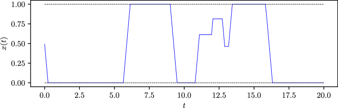
Figure 3: Realization of $x$ for the CITP with $\omega=0.5$ and $\ell=1$

In order to emphasize which $\sigma^{i}$, $x_{0}$ and $\ell$ were used, the process constructed in the previous definition is sometimes denoted by $\mathcal{X}(\sigma^{1},\sigma^{2},x_{0},\ell)$. When the $\sigma^{i}$ follow the rates of figure 2(a), $X$ is called the continuous instantaneous tumble process (CITP) and when the $\sigma^{i}$ follow the rates of figure 2(b), $X$ is called the continuous finite tumble process (CFTP).

Starting from definition 2, the proof of the strong Markov property and the characterization of the generator requires careful work. Instead, as done in [HGM23], we construct the process using the formalism of piecewise deterministic Markov processes (PDMPs) developed in [Dav93] so that the strong Markov property and the characterization of the generator are immediate. As done in [Bie+23], a bijection $\iota$ mapping the state space of the PDMP to a more convenient state space is used to come back to definition 2. It is the subject of Section 2.

1.2.3 Main results

The following theorem is a summary of the findings obtained in this paper.

Theorem 1.

Let $\gamma_{L}=(L-1)/\ell$.

1. The discrete in space processes DITP (resp. DFTP) converge, with quantitative control, when $L$ tends to infinity, in Skorohod topology towards the continuous-space piecewise deterministic Markov process CITP (resp. CFTP).

2. The processes DITP and DFTP are exponentially ergodic with invariant measures converging as $L$ tends to infinity to the unique invariant measures of the CITP and CFTP.

3. The invariant measures of CITP and CFTP have a positive mass at $\{0\}\times\{-1,0,1\}$ and $\{\ell\}\times\{-1,0,1\}$.

4. Let us define for a Markov process with semigroup $P_{t}$ and invariant measure $\pi$ its mixing time as $t_{\text{mix}}(\epsilon)=\inf\left\{t\geq 0\,;\,sup_{\mu}\|\mu P_{t}-\pi\|_{TV}\leq\epsilon\right\}$.

   1. The mixing time $t_{\text{mix}}(\epsilon)$ of CITP is of the order $C^{\prime}(\epsilon)\frac{1}{\omega}(1+\omega^{2}l^{2})$ for some $C^{\prime}(\epsilon)$.

   2. The mixing time $t_{\text{mix}}(\epsilon)$ of CFTP is of the order $C^{\prime}(\epsilon)(\frac{1}{\alpha}+\frac{1}{\beta})(1+\alpha^{2}l^{2})$ for some $C^{\prime}(\epsilon)$.

The precise statements of points (1)–(3) are given in Theorem 2, Corollary 1 and in the appendix. It enables to justify the analysis of [SEB16, SEB17] who have calculated the invariant measure of the DITP and DFTP and have passed to the limit in order to assert that this processes exhibit a MIPS phenomenon, i.e. only their intrinsic movement allows for agglomerate of particles asserted by a positive mass at $0$ and $\ell$. This result not only ensures the validity of their analysis but also provides a direct way to build processes (PDMPs) at the continuous level. Note that the explicit invariant measures obtained in the Appendix is a particular case of the general study of [HGM23] where universality classes (for the invariant measures) were derived for general pairs of RTPs depending on the behavior at the jamming boundary. The coupling strategy used here to derive the discrete to continuous limit is quite general and is not limited to the DITP/DFTP processes of [SEB16, SEB17].

The mixing times were not studied before, despite the importance of the understanding of the speed of convergence to stationarity. The precise statements of the results are given in Theorem 3. Most interestingly, it reveals two regimes controlled by the parameter $\omega\ell$ for the CITP

• the persistent regime $\omega\ell\ll 1$ where the mean time between two stochastic velocity changes is much greater than the time needed to reach a jammed configuration,

• the diffusive regime $\omega\ell\gg 1$ where the mean time between two stochastic velocity changes is much lower than the time needed to reach a jammed configuration.

This allows for a heuristic interpretation of the mixing time in terms of slow observables. In the persistent regime, the slowest observables are the velocities $\sigma^{i}$ so the mixing time is of order $1/\omega$. In the diffusive regime, the position $x$ is the slowest observable and its dynamic is approximately Brownian leading to the mixing time $\omega\ell^{2}$ with the quadratic dependence in $\ell$ characteristic of diffusions.

For the CFTP, the mixing time is the product of $\frac{1}{\alpha}+\frac{1}{\beta}$, the average time needed to see a velocity flip of each kind, and $1+\alpha^{2}\ell^{2}$ which accounts for the possibly diffusive behavior. Notice that the mixing times in theorem 1 (4) are coherent with the fact that, when $\beta\to+\infty$, the CFTP becomes the CITP with $\omega=\alpha/2$.

1.2.4 Plan of the paper

In the following, the stochastic processes CITP and CFTP are constructed in section 2 considering the PDMP formulation of Davis [Dav93], with a particular emphasis on their generator. The continuous PDMP description proves helpful to derive the explicit form of the invariant measure, as was generally done in [HGM23], but also for mixing time evaluation. In section 3, it is shown that, under the right rescaling, the discrete process converges in law to the continuous process with respect to the Skorokhod metric. It is also proven that the on-lattice invariant measures converge to the continuous invariant measure with respect to the Wasserstein distance. Proofs are based on coupling between the discrete state process and the continuous one. In section 4, the scaling of the mixing time of the continuous process as a function of model parameters is determined. The arguments leading to such precise controls on the mixing time relies on sharp controls of expectation of particular hitting times of the continuous-space processes, as well as concentration of additive functionals of the velocity processes. Finally, for the sake of completeness, the explicit formula for the invariant measure of the continuous processes is recalled in the appendix, directly for CITP and CFTP, using a similar but alternative approach to that in [HGM23].

2 PDMP formulation of the continuous-space processes

Piecewise deterministic Markov processes are characterized by a deterministic dynamic interspersed with random jumps. Their appeal lies in the wide range of processes that fall into this category and their straightforward construction. The complete characterization of their generator and its domain is known, even if sometimes in an intrinsic way. This greatly facilitates the search for their invariant measures. Furthermore, the formalism conveniently includes a way of explicitly computing the expected value and the Laplace transform of hitting times by solving systems of differential equations.

In [HGM23], the goal is to derive the invariant measure for the two RTP in a general setting. Therefore the considered PDMP encodes all the system symmetries (particle indistinguishability, periodicity, space homogeneity) and thus corresponds to the evolution of the interdistance between the two particles. Here, we are interested in the limit of the discrete process $Y^{L}$ studied in [SEB16, SEB17] and the mixing behavior for the particular case of the instantaneous and finite tumbles. Therefore we construct following [Dav93] the PDMP describing the evolution of $(x,\nu)$ with $x\in[0,\ell]$ the inter-particle separation, as previously defined, for the 2-RTP system with instantaneous tumbles (resp. finite tumbles) and $\nu\in K$ a variable ruling the deterministic dynamics. We first describe the state space and deterministic dynamics. The process takes its values in the state space $E_{D}=\bigcup_{\nu\in K}E_{\nu}$ which can be divided into a bulk and a boundary as follows

• the bulk $\cup_{\nu\in K\setminus\partial K}E_{\nu}$ corresponds to states where

  • $0<x<\ell$ meaning that the particles are at positive distance and the deterministic dynamics corresponds to the ODE $\partial_{t}x=\sigma^{2}-\sigma^{1}$ (ex: figure 4(a)),

  • $x\in\{0,\ell\}$ meaning that the particles are at contact and their velocities push them apart (ex: figure 4(b)),

• the boundary $\cup_{\nu\in\partial K}E_{\nu}$ corresponds to states where $x\in\{0,\ell\}$ meaning that the particles are at contact and their velocities push them together so they jam (ex: figure 4(c)). In the jammed states of the boundary, the distance $x$ is constant.

Thus, the variable $\nu$ encodes both the value of the velocities $\sigma^{i}$ and whether or not the particles are jammed.

(a) $0<x<\ell$ and $\nu=(-1,1)$

(b) $x=\ell$ and $\nu={(1,-1)}$

(c) $x=\ell$ and $\nu=*^{\ell}_{(-1,1)}$

Figure 4: Bulk and boundary states of the continuous process

Therefore we set $\Sigma=\{-1,1\}^{2}$ (resp. $\Sigma=\{-1,0,1\}^{2}$) as well as

$$\Sigma_{+}=\{(\sigma^{1},\sigma^{2})\in\Sigma:\sigma^{2}-\sigma^{1}\geq 0\}\text{ and }\Sigma_{-}=\{(\sigma^{1},\sigma^{2})\in\Sigma:\sigma^{2}-\sigma^{1}\leq 0\},$$

and we define $\partial K=\left\{*^{\ell}_{\sigma}:\sigma\in\Sigma_{+}\right\}\cup\left\{*^{0}_{\sigma}:\sigma\in\Sigma_{-}\right\}$ and $K=\Sigma\cup\partial K$. The state space $E_{D}$ is built from the family of measurable sets $(E^{0}_{\nu})_{\nu\in K}$ defined by

$$E_{\sigma}^{0}=(0,\ell)\times\left\{\sigma\right\}\text{ for }\sigma\in\Sigma,\quad\quad E_{*_{\sigma}^{\ell}}^{0}=\{\ell\}\times\left\{*^{\ell}_{\sigma}\right\}\text{ for }\sigma\in\Sigma_{+},\quad\quad E_{*_{\sigma}^{0}}^{0}=\{0\}\times\left\{*^{0}_{\sigma}\right\}\text{ for }\sigma\in\Sigma_{-}.$$

We consider the family of vector fields $(\mathfrak{X}_{\nu})_{\nu\in K}$ where

• for $\sigma\in\Sigma$ the vector field $\mathfrak{X}_{\sigma}$ defined on $E^{0}_{\sigma}$ corresponds to the ODE $\partial_{t}x=\sigma^{2}-\sigma^{1}$,

• for $\nu\in\partial K$ the vector field $\mathfrak{X}_{\nu}$ defined on $E^{0}_{\nu}$ is null.

The sets $E^{0}_{\nu},\nu\in\partial K$ include the sticky points of the dynamics, here corresponding to jamming configurations, and come down to singletons for $x$. Further details on the extension of the formalism of Davis to include such sets can be found in [Bie+23].

Adding the entry-non-exit points, we get the family of measurable sets $(E_{\nu})_{\nu\in K}$ defined by

• $E_{(\sigma^{1},\sigma^{2})}=[0,\ell)\times\{(\sigma^{1},\sigma^{2})\}$ for $(\sigma^{1},\sigma^{2})\in\Sigma$ such that $\sigma^{2}-\sigma^{1}>0$,

• $E_{(\sigma^{1},\sigma^{2})}=(0,\ell)\times\{(\sigma^{1},\sigma^{2})\}$ for $(\sigma^{1},\sigma^{2})\in\Sigma$ such that $\sigma^{2}-\sigma^{1}=0$,

• $E_{(\sigma^{1},\sigma^{2})}=(0,\ell]\times\{(\sigma^{1},\sigma^{2})\}$ for $(\sigma^{1},\sigma^{2})\in\Sigma$ such that $\sigma^{2}-\sigma^{1}<0$,

• $E_{\nu}=E^{0}_{\nu}$ for $\nu\in\partial K$,

forming up $E_{D}=\bigcup_{\nu\in K}E_{\nu}$.

We now define the stochastic jumps. We recall that the states $(x,(\sigma^{1},\sigma^{2})),(0,*^{0}_{(\sigma^{1},\sigma^{2})})$ and $(\ell,*^{\ell}_{(\sigma^{1},\sigma^{2})})$ all correspond to the first particle having velocity $\sigma^{1}$ and the second particle having velocity $\sigma^{2}$. The velocities of the particles are independent Markov jump processes with the transition rates of figure 2(a) (resp. 2(b)) and we define $\mathcal{Q}=(q_{\sigma,\sigma^{\prime}})_{\sigma,\sigma^{\prime}\in\Sigma}$ as the discrete generator of the couple $(\sigma^{1},\sigma^{2})$. For example, if the $\sigma^{i}$ follow figure 2(a) then

$$\mathcal{Q}=\bordermatrix{&\sigma^{\prime}=(1,1)&\sigma^{\prime}=(1,-1)&\sigma^{\prime}=(-1,1)&\sigma^{\prime}=(-1,-1)\cr\sigma=(1,1)&-2\omega&\omega&\omega&0\cr\sigma=(1,-1)&\omega&-2\omega&0&\omega\cr\sigma=(-1,1)&\omega&0&-2\omega&\omega\cr\sigma=(-1,-1)&0&\omega&\omega&-2\omega}.$$

We introduce the following projectors.

Definition 3.

Define $p_{\sigma^{1}}:E_{D}\rightarrow\{-1,1\}$ (resp. $\{-1,0,1\}$) and $p_{\sigma^{2}}:E_{D}\rightarrow\{-1,1\}$ (resp. $\{-1,0,1\}$) by

$$p_{\sigma^{1}}\left(x,\nu\right) =\sum_{(\sigma^{1},\sigma^{2})\in\Sigma}\sigma^{1}1_{\{(\sigma^{1},\sigma^{2}),*^{0}_{(\sigma^{1},\sigma^{2})},*^{\ell}_{(\sigma^{1},\sigma^{2})}\}}(\nu),$$

$$p_{\sigma^{2}}\left(x,\nu\right) =\sum_{(\sigma^{1},\sigma^{2})\in\Sigma}\sigma^{2}1_{\{(\sigma^{1},\sigma^{2}),*^{0}_{(\sigma^{1},\sigma^{2})},*^{\ell}_{(\sigma^{1},\sigma^{2})}\}}(\nu).$$

and $p_{\sigma}$ by

$$p_{\sigma}\left(x,\nu\right)=(p_{\sigma^{1}}\left(x,\nu\right),p_{\sigma^{2}}\left(x,\nu\right)).$$

For $(x,\nu)\in E_{D}$, we define the jump rate $\lambda$ by $\lambda(x,\nu)=-q_{p_{\sigma}(x,\nu),p_{\sigma}(x,\nu)}$ and the jump kernel by

$$Q((x,\nu);\cdot)=\sum_{\nu^{\prime}\in K}-\frac{q_{p_{\sigma}(x,\nu),p_{\sigma}(x,\nu^{\prime})}}{q_{p_{\sigma}(x,\nu),p_{\sigma}(x,\nu)}}1_{E_{D}}((x,\nu^{\prime}))\delta_{(x,\nu^{\prime})}.$$

As exactly one of the elements of $\{(x,\sigma^{\prime});(x,*_{\sigma^{\prime}}^{0});(x,*_{\sigma^{\prime}}^{\ell})\}$ is in the state space $E_{D}$, $Q((x,\nu);\cdot)$ is indeed a probability measure.

It remains to define the boundary jumps: When the deterministic dynamics leads to a state where the particles are jammed, the process jumps to the corresponding boundary state. On the exit boundary $\Gamma^{*}=\{(0,\sigma):\sigma\in\Sigma_{-}-\Sigma_{+}\}\cup\{(\ell,\sigma):\sigma\in\Sigma_{+}-\Sigma_{-}\}$, the jump kernel is given by

$$Q((0,\sigma);\cdot)=\delta_{(0,*_{\sigma}^{0})}\text{ for }\sigma\in\Sigma_{-}-\Sigma_{+}\text{ and }Q((\ell,\sigma);\cdot)=\delta_{(\ell,*_{\sigma}^{\ell})}\text{ for }\sigma\in\Sigma_{+}-\Sigma_{-}.$$

Many important properties of PDMPs, such as the characterization of their generator, are true under the set of ‘standard conditions’ (24.8) of [Dav93]. The continuous process clearly satisfies conditions (1)–(3) and condition (4) follows from proposition (24.6) of [Dav93]. Theorem (26.14) of [Dav93] hence yields the following characterization of the generator.

Proposition 1 (Generator of the continuous process).

Let $\mathcal{L}$ be the generator of the continuous process. Its domain $D(\mathcal{L})$ is the set of bounded measurable functions $f:E_{D}\rightarrow\mathbb{R}$ such that

• for $\sigma\in\Sigma_{+}-\Sigma_{-}$ the function $f(\cdot,\sigma)$ is absolutely continuous on $[0,\ell)$ and $\lim_{x\rightarrow\ell}f(x,\sigma)=f\left(\ell,*_{\sigma}^{\ell}\right)$,

• for $\sigma\in\Sigma_{-}-\Sigma_{+}$ the function $f(\cdot,\sigma)$ is absolutely continuous on $(0,\ell]$ and $\lim_{x\rightarrow 0}f(x,\sigma)=f\left(0,*_{\sigma}^{0}\right)$.

For $f\in D(\mathcal{L})$ one has that

• in the bulk $\cup_{\sigma\in\Sigma}E_{\sigma}$ the generator comprises a transport term and a jump term

  $$\mathcal{L}f(x,(\sigma^{1},\sigma^{2})) =\underbrace{(\sigma^{2}-\sigma^{1})\partial_{x}f(x,(\sigma^{1},\sigma^{2}))}_{\text{transport term}}$$

  $$\qquad+\underbrace{\lambda(x,\nu)\int_{E}\left(f(\tilde{x},\tilde{\nu})-f(x,(\sigma^{1},\sigma^{2}))\right)dQ\left((x,(\sigma^{1},\sigma^{2}));(\tilde{x},\tilde{\nu})\right)}_{\text{jump term}},$$

• whereas for boundary states $(x,\nu)\in\cup_{\nu\in\partial K}E_{\nu}$ the generator is given only by the jump term

  $$\mathcal{L}f(x,\nu)=\lambda(x,\nu)\int_{E}\left(f(\tilde{x},\tilde{\nu})-f(x,\nu)\right)dQ((x,\nu);(\tilde{x},\tilde{\nu}))$$

To emphasize the difference with definition 2, we denote this process $X_{D}(t)=(x(t),\nu(t))$. Formally, definition 2 and the PDMP construction model the same process, but differ on the choice of the dynamics variable. Indeed, the vector fields $(\mathfrak{X}_{\nu})_{\nu\in K}$ have to be continuous, hence the consideration of $\nu$ and its additional states forming up $\partial K$. Out of completeness, we rigorously establish such link, so as to be able to use them both.

Definition 4.

Define $\iota:E_{D}\rightarrow[0,\ell]\times\Sigma$ by

$$\iota(x,\nu)=\left(x,p_{\sigma}(x,\nu)\right).$$

Proposition 2.

The mapping $\iota$ is a bijection.

Proof.

This follows from the fact that for all $x\in[0,\ell]$ and all $\sigma=(\sigma^{1},\sigma^{2})\in\Sigma$ exactly one element among $(x,\sigma),(x,*_{\sigma}^{0}),(x,*_{\sigma}^{\ell})$ is defined and an element of $E_{D}$. Indeed,

• if $x\in(0,\ell)$ then $(x,\sigma)\in E_{D}$ and $(x,*^{0}_{\sigma})\not\in E_{D}$ for $\sigma\in\Sigma_{-}$, $(x,*^{\ell}_{\sigma})\not\in E_{D}$ for $\sigma\in\Sigma_{+}$,

• if $x=0$ then

  • if $\sigma^{2}-\sigma^{1}>0$ then $(0,\sigma)\in E_{D}$ and $(0,*^{\ell}_{\sigma})\not\in E_{D}$,

  • if $\sigma^{2}-\sigma^{1}\leq 0$ then $(0,*^{0}_{\sigma})\in E_{D}$ and $\{(0,\sigma);(0,*^{\ell}_{\sigma})\}\cap E_{D}=\emptyset$,

• if $x=\ell$

  • if $\sigma^{2}-\sigma^{1}<0$ then $(\ell,\sigma)\in E_{D}$ and $(\ell,*^{0}_{\sigma})\not\in E_{D}$,

  • if $\sigma^{2}-\sigma^{1}\geq 0$ then $(\ell,*^{\ell}_{\sigma})\in E_{D}$ and $\{(\ell,\sigma);(\ell,*^{0}_{\sigma})\}\cap E_{D}=\emptyset$.

∎

Proposition 3.

Let $X_{D}(t)=(x(t),\nu(t))$ be as in Section 2.

• The processes $\sigma^{1}(t)=p_{\sigma^{1}}(X_{D}(t))$ and $\sigma^{2}(t)=p_{\sigma^{2}}(X_{D}(t))$ are two independent Markov jump processes with the transition rates of figure 2(a) (resp. 2(b)).

• If one recursively defines

  $$\tilde{x}(t)=\max\left[0,\min\left[\ell,\tilde{x}({T_{n}})+(\sigma^{2}(t)-\sigma^{1}(t))(t-T_{n})\right]\right]\text{ for }T_{n}\leq t\leq T_{n+1}$$

  where $0=T_{0}<T_{1}<\cdots$ are the jump times of the couple $(\sigma^{1},\sigma^{2})$ then $\iota(X_{D}(t))=(\tilde{x}(t),(\sigma^{1}(t),\sigma^{2}(t)))$.

Proof.

(i) For all fixed $(s^{1},s^{2})\in\Sigma$ the function $f(x,\nu)=\mathbb{P}_{(x,\nu)}\left(p_{\sigma}(X_{D}(t))=(s^{1},s^{2})\right)$ can be computed explicitly using its characterization as the solution of a system of differential equations (see section 3 of [Dav93]). One gets

$$\mathbb{P}_{(x,\nu)}\left(p_{\sigma}(X_{D}(t))=(s^{1},s^{2})\right)=\mathbb{P}_{p_{\sigma^{1}}(x,\nu)}\left(\varsigma_{1}(t)=s_{1}\right)\mathbb{P}_{p_{\sigma^{2}}(x,\nu)}\left(\varsigma_{2}(t)=s_{2}\right)\text{ for all }(s_{1},s_{2})\in\Sigma$$

where the $\varsigma_{i}$ are Markov jump processes with the transition rates of figure 2(a) (resp. 2(b)).

(ii) Follows from the recursive construction in section 23 of [Dav93]. ∎

3 From discrete to continuous space

3.1 Convergence in law

In this section, it is shown that under the right rescaling the discrete process of [SEB16, SEB17], i.e. DITP (resp. DFTP), converges to the continuous process CITP (resp. CFTP).

First, the discrete and continuous process have different state spaces. The continuous process $X$ takes its values in $[0,\ell]\times\Sigma$ and one can think of $\{1,\ldots L\}$ as a discrete subset of the interval $[0,\ell]$ using the injection

$$i_{L}(k):=\ell\frac{k-1}{L-1}.$$

This allows one to see the discrete process as taking values in $[0,\ell]\times\Sigma$ and to consider the process $(i_{L}(y^{L}(t)),(\sigma^{1}(t),\sigma^{2}(t)))$ instead of $(y^{L}(t),(\sigma^{1}(t),\sigma^{2}(t)))$.

It remains to understand how the parameters $\omega$ (resp. $\alpha$ and $\beta$), $\gamma$ and $L$ should scale. Thinking of the discrete process as an approximation of the continuous process where the interval $[0,\ell]$ is replaced by its discrete counterpart $\{1,\ldots,L\}$, the natural scalings

L→+∞γL=(L−1)/ℓ\displaystyle(*)\left\{\begin{tabular}[]{c}$\omega$ (resp. $\alpha$ and $\beta$) constant\\ $L\rightarrow+\infty$\\ $\gamma_{L}=(L-1)/\ell$\end{tabular}\right.

$(\ast )\{\begin{array}{c}\end{array}$ ω (resp. α and β) constant

correspond to taking increasingly fine discretisations of the position $y^{L}(t)$ while preserving the dynamics of the $\sigma^{i}$ and the physical velocity of the particles $\ell\gamma/(L-1)$.

The convergence of Markov processes is often shown using approaches based on generators or on martingale problems (see [EK86]). Here, we take a different approach and instead use a coupling argument. It requires only basic probabilistic tools and also provides quantitative estimates for the approximation procedure. The key insight is that, under the scalings described above, the stochastic jumps of $y^{L}(t)$ become both smaller in size and more frequent in a way that makes them converge to the constant velocity translations of $x(t)$.

Theorem 2 (Scaling limit).

• There exists a coupling of the continuous process $X$ and a sequence of discrete processes $(Y^{L})_{L\geq 2}$ with parameters scaling as in ($*$) such that for all $T>0$

  $$\mathbb{P}\left(\sup_{t\leq T}\left|i_{L}(y^{L}(t))-x(t)\right|\geq\epsilon\right)\leq\frac{1}{\epsilon}\left(\frac{\ell}{L-1}+8\sqrt{\frac{T\left((\eta T)^{2}+3\eta T+1\right)\ell}{L-1}}\right)$$

  where $\eta=2\omega$ (resp. $\eta=2\max(\alpha,\beta)$) for the instantaneous-tumble transition rates of the $\sigma^{i}$ (resp. the finite-tumble transition rates).

• One has

  $$\Big{(}(i_{L}(y^{L}(t)),(\sigma^{1}(t),\sigma^{2}(t)))\Big{)}_{t\geq 0}\overset{\text{Law}}{\longrightarrow}\Big{(}X(t)\Big{)}_{t\geq 0}$$

  in the Skorokhod space $\mathcal{D}[0,+\infty)$.

As the supremum distance is finer than the Skorokhod distance, assertion (i) implies that for all $T>0$

$$\Big{(}(i_{L}(y^{L}(t)),(\sigma^{1}(t),\sigma^{2}(t)))\Big{)}_{t\in[0,T]}\overset{\text{Law}}{\longrightarrow}\Big{(}X(t)\Big{)}_{t\in[0,T]}$$

in the sense of random variables taking their values in the Skorokhod space $\mathcal{D}[0,T]$. Hence assertion (ii) follows by theorem 16.7 of [Bil99]. Therefore, the rest of this subsection is dedicated to the proof of assertion (i).

The jamming mechanism at $y^{L}=1$ and $y^{L}=L$ makes the control of $(i_{L}(y^{L}(t))-x(t))$ challenging. Therefore, we first consider the following simplified model, without any jamming and taking values in $\mathbb{Z}$. For this model, we derive a uniform bound similar to the one of assertion (i) in theorem 2.

Lemma 1.

Let $\sigma^{1}$ and $\sigma^{2}$ be two independent Markov jump processes with the transition rates of figure 2(a) (resp. 2(b)) and let $N_{1}^{L}$ and $N_{2}^{L}$ be two independent Poisson processes with rate $\gamma_{L}$ independent of the $\sigma^{i}$.

If one sets

$$S^{L}(t)=\sum_{s\leq t}\sum_{i=1,2}1_{\{N_{i}^{L}(s+)\neq N_{i}^{L}(s-)\}}(-1)^{i}\sigma^{i}(s)\ \text{and}\ I(t):=\int_{0}^{t}(\sigma^{2}(s)-\sigma^{1}(s))ds.$$

then one has

$$\mathbb{P}\left(\sup_{t\leq T}\left|\frac{1}{\gamma_{L}}S^{L}(t)-I(t)\right|\geq\epsilon\right)\leq\frac{2}{\epsilon}\sqrt{\frac{T}{\gamma_{L}}}.$$

The proof is included for the sake of completeness.

Proof.

First, $(S^{L}(t),(\sigma^{1}(t),\sigma^{2}(t)))$ is a $(\mathbb{Z}\times\Sigma)$-valued Markov jump process and its generator $\mathcal{L}^{L}$ is given by

$$\mathcal{L}^{L}f(z,(\sigma^{1},\sigma^{2}))=\gamma_{L}\big{(}f(z-\sigma^{1},(\sigma^{1},\sigma^{2}))+f(z+\sigma^{2},(\sigma^{1},\sigma^{2}))-2f(z,(\sigma^{1},\sigma^{2})\big{)}\\ +\sum_{(s^{1},s^{2})\in\Sigma}q_{(\sigma^{1},\sigma^{2}),(s^{1},s^{2})}f(z,(s^{1},s^{2}))$$

where $\mathcal{Q}=(q_{\sigma,\sigma^{\prime}})_{\sigma,\sigma^{\prime}\in\Sigma}$ is the generator of the couple $(\sigma^{1},\sigma^{2})$, as defined in the previous Section. Hence Dynkin’s formula implies that $S^{L}(t)-\gamma_{L}\int_{0}^{t}(\sigma^{2}(s)-\sigma^{1}(s))ds$ is a martingale and by Doob’s martingale inequality

$$\mathbb{P}\left(\sup_{t\leq T}\left|\frac{1}{\gamma_{L}}S^{L}(t)-I(t)\right|\geq\epsilon\right)$$

$$\qquad\qquad\qquad\leq\frac{\mathbb{E}\left|S^{L}(T)-\gamma_{L}I(T)\right|}{\epsilon\gamma_{L}},$$

$$\qquad\qquad\qquad\leq\frac{\sum_{i=1,2}\mathbb{E}\left|\sum_{s\leq T}1_{\{N_{i}^{L}(s+)\neq N_{i}^{L}(s-)\}}\sigma^{i}(s)-\gamma_{L}\int_{0}^{T}\sigma^{i}(s)ds\right|}{\epsilon\gamma_{L}},$$

$$\qquad\qquad\qquad\leq\frac{2}{\epsilon\gamma_{L}}\sqrt{\mathbb{E}\left(\sum_{s\leq T}1_{\{N_{1}^{L}(s+)\neq N_{1}^{L}(s-)\}}\sigma^{1}(s)-\gamma_{L}\int_{0}^{T}\sigma^{1}(s)ds\right)^{2}}.$$

It remains to show that $\mathbb{E}\left(\sum_{s\leq T}1_{\{N_{1}^{L}(s+)\neq N_{1}^{L}(s-)\}}\sigma^{1}(s)-\gamma_{L}\int_{0}^{T}\sigma^{1}(s)ds\right)^{2}\leq T\gamma_{L}$. Let $(T_{n})_{n\geq 0}$ be the jump times of the couple $(\sigma^{1},\sigma^{2})$. The process $M(t)=\sum_{s\leq t}1_{\{N_{1}^{L}(s+)\neq N_{1}^{L}(s-)\}}\sigma^{1}(s)-\gamma_{L}\int_{0}^{t}\sigma^{1}(s)ds$ is also a martingale by Dynkin’s formula so that repeated use of the optional stopping theorem yields

$$\mathbb{E}\left[M(T)^{2}\right]=\sum_{k=1}^{N}\mathbb{E}\left[(M(T_{k}\wedge T)-M(T_{k-1}\wedge T))^{2}\right]+\mathbb{E}\left[(M(T)-M(T_{N}\wedge T))^{2}\right].$$

Taking $N\rightarrow+\infty$ and using the dominated convergence theorem one gets

$$\mathbb{E}\left[(M(T)-M(T\wedge T_{N}))^{2}\right]\rightarrow 0$$

and $\mathbb{E}\left[M(T)^{2}\right]=\sum_{k=1}^{+\infty}\mathbb{E}\left[(M(T_{k}\wedge T)-M(T_{k-1}\wedge T))^{2}\right]$ so that

$$\mathbb{E}\left[M(T)^{2}\right] =\sum_{k=1}^{+\infty}\mathbb{E}\left[\sigma^{1}(T_{k-1}\wedge T)^{2}(N_{1}^{L}(T_{k}\wedge T)-N_{1}^{L}(T_{k-1}\wedge T)-\gamma_{L}(T_{k}\wedge T-T_{k-1}\wedge T))^{2}\right],$$

$$\leq\sum_{k=1}^{+\infty}\mathbb{E}\left[\left(N_{1}^{L}(T_{k}\wedge T)-N_{1}^{L}(T_{k-1}\wedge T)-\gamma_{L}(T_{k}\wedge T-T_{k-1}\wedge T)\right)^{2}\right]$$

$$=\mathbb{E}\left[\left(N_{1}^{L}(T)-\gamma_{L}T\right)^{2}\right]=\gamma_{L}T.$$

∎

Remark 1.

It is easy to see that one can also directly obtain an upper bound in the previous lemma such as $8T/(\epsilon^{2}\gamma_{L})$ (in fact even exponential inequality can be derived). This bound worsens with respect to $T$, but exhibits improved behavior with respect to $\gamma_{L}$.

Formally, for $\gamma_{L}\rightarrow+\infty$, the jumps of $S^{L}/\gamma_{L}$ have decreasing size $1/\gamma_{L}$ but increasing rate $\gamma_{L}$ so that the physical velocity $\gamma_{L}/\gamma_{L}=1$ remains constant. Lemma 1 rigorously implies that the stochastic jumps of $S^{L}/\gamma_{L}$ converge to the constant velocity translations of $I(t)$ with the supremum norm, thanks to Doob’s martingale inequality.

We now introduce the following coupling to prove the convergence of the discrete process to the continuous process, i.e. assertion (i) of the theorem 2, by drawing on the lines of the proof of lemma 1.

Definition 5 (Discrete-continuous coupling).

Let $X(t)=(x(t),(\sigma^{1}(t),\sigma^{2}(t)))$ be a continuous process as defined in definition 2, with fixed parameters $\omega$ (resp. $\alpha$ and $\beta$) and $\ell$, and $\sigma^{1}(t)$ and $\sigma^{2}(t)$ two independent Markov jump processes with the transition rates of figure 2(a) (resp. 2(b)). Denote by $0=T_{0}<T_{1}<\cdots$ the jump times of the couple $(\sigma^{1},\sigma^{2})$. For $L\geq 2$, let $N_{1}^{L}$ and $N_{2}^{L}$ be two independent Poisson processes with parameter $\gamma_{L}=(L-1)/\ell$ independent of the $\sigma^{i}$.

Recursively define $y^{L}$ by setting

$$y^{L}(0)=\left\lfloor(L-1)x(0)/\ell\right\rfloor+1\ \text{and}\ z^{L}(t):=y^{L}(T_{k})+\sum_{i=1,2}(-1)^{i}\sigma^{i}(T_{k})\left[N^{L}_{i}(t)-N^{L}_{i}(T_{k})\right],$$

• if $(\sigma^{1}(T_{k}),\sigma^{2}(T_{k}))\neq\pm(1,1)$

  $$y^{L}(t)=\max\left[1,\min\left[L,z^{L}(t)\right]\right]\text{ for }t\in[T_{k},T_{k+1}],$$

• if $(\sigma^{1}(T_{k}),\sigma^{2}(T_{k}))=\pm(1,1)$

  $$y^{L}(t)=p_{L}\left(z^{L}(t)\right)\text{ for }t\in[T_{k},T_{k+1}]$$

  where $p_{L}:\mathbb{Z}\rightarrow\{1,\ldots,L\}$ is given by

  $$p_{L}(k+2mL)=\left\{\begin{array}[]{cl}k&\text{ for }m\in\mathbb{Z}\text{ and }1\leq k\leq L,\\ 2L+1-k&\text{ for }m\in\mathbb{Z}\text{ and }L+1\leq k\leq 2L.\end{array}\right.$$

Finally, set $Y^{L}(t)=(y^{L}(t),(\sigma^{1}(t),\sigma^{2}(t)))$.

The construction in definition 5 of $Y^{L}$ using $p_{L}$ differs from definition 1. The goal of this coupling is to map the transitions of the DITP (resp. DFTP) to the jamming-free random walk $z^{L}$, that was already studied in the toy model of lemma 2. The difference lies in the case $\sigma^{1}=\sigma^{2}=\pm 1$. A definition through the $\max(\min(\cdot))$ definition is not correct at jamming, as the $y^{L}$ is evaluated and fixed at its $t=T_{k}$ value. However, the definition through $p^{L}$ ensures a correct mapping by exploiting the indistinguishability of the particles (i.e. the Poisson process $N^{L}_{1}$ (resp. $N^{L}_{2}$) does not correspond to the Poisson clock linked to particle $1$ (resp. $2$)). In more details, in such case, the process $y^{L}$ comes down to a symmetric random walk (see figure 5), that is mapped to the symmetric random walk $z^{L}$ in this manner:

• Case $p_{L}(z^{L})=y^{L}\notin\{1,L\}$; If $z^{L}$ jumps left (resp. right) with rate $\gamma_{L}$, then $p_{L}$ maps this to the left (resp. right) jump of $y^{L}$.

• Case $p_{L}(z^{L})=y^{L}\in\{1,L\}$, say $z^{L}=y^{L}=L$; If $z^{L}$ jumps to $L-1$ with rate $\gamma_{L}$, then $p_{L}$ maps this to the jump of $y^{L}$ to $L-1$. If $z^{L}$ jumps to $L+1$, the value of $p_{L}(z^{L})$ stalls at $L$ and $y^{L}$ does not jump.

While the actual proof of the mapping is required, such mapping enables a direct derivation of the convergence bound. Indeed, it now appears possible to bound $\sup_{t\leq T}\left|i_{L}(y^{L}(t))-x(t)\right|$ in terms of $\sup_{t\leq T}|N_{i}^{L}(t)-\gamma_{L}t|$. Hence, because $(N_{i}^{L}(t)-\gamma_{L}t)$ is a martingale, a uniform bound similar to lemma 1 is attainable.

Figure 5: Transition rates of the DITP (resp. DFTP) conditionned on $\sigma^{1}=\sigma^{2}=\pm 1$

Lemma 2.

Let $X$ and the sequence of stochastic processes $(Y^{L})_{L\geq 2}$ be as in definition 5.

• Each $Y^{L}$ is a DITP (resp. DFTP).

• Let $0=T_{0}<T_{1}<\cdots$ be the jump times of the couple $(\sigma^{1},\sigma^{2})$. For all $t\geq 0$ one has

  $$\left|i_{L}(y^{L}(t))-x(t)\right|\leq \left|i_{L}(y^{L}(0))-x(0)\right|+\frac{1}{\gamma_{L}}\sum_{k=1}^{n(t)}\left|D_{k}(t)\right|$$

  where $n(t)=1+\sum_{k=1}^{+\infty}1_{\{T_{k}\leq t\}}$ and

  $$D_{k}(t)=\sum_{i=1,2}(-1)^{i}\sigma^{i}(T_{k-1})\Big{[}N_{i}^{L}(T_{k}\wedge t)-N_{i}^{L}(T_{k-1}\wedge t)-\gamma_{L}\left(T_{k}\wedge t-T_{k-1}\wedge t\right)\Big{]}.$$

Proof.

(i) First prove that the definition 5 indeed provides a coupling, i.e. $Y^{L}$ alone is indeed a DITP (or DFTP).

Let $L\geq 2$ be arbitrary but fixed. Let $Y^{L}$ be as in definition 5 and let $\sigma^{i}$ and $N_{i}^{L}$ be the corresponding velocities and Poisson processes. Set $\tilde{Y}^{L}=\mathcal{Y}(\sigma^{1},\sigma^{2},N_{1}^{L},N_{2}^{L},L)$.

To show that $Y^{L}$ and $\tilde{Y}^{L}$ have the same law, it suffices to show that $y^{L}$ and $\tilde{y}^{L}$ are identically distributed conditional on the velocities $(\sigma^{1},\sigma^{2})$. Let $s:[0,+\infty)\rightarrow\Sigma$ be an arbitrary but fixed càdlàg function. In the remainder of the proof of (i), take the conditional probability $\mathbb{Q}=\mathbb{P}\left(\cdot\,|\,(\sigma^{1},\sigma^{2})=s\right)$ to be the reference probability so that functionals of the $\sigma^{i}$ such as jump times are deterministic. Under the probability $\mathbb{Q}$ both $y^{L}$ and $\tilde{y}^{L}$ are time-inhomogeneous Markov processes with the same initial distribution so that it suffices to prove that their transition probabilities are the same.

Recall that $0=T_{0}<T_{1}<\cdots$ are the jump times of the couple $(\sigma^{1},\sigma^{2})$. For $t\in[T_{k},T_{k+1}]$,

• if $(\sigma^{1}(T_{k}),\sigma^{2}(T_{k}))\neq\pm(1,1)$ then

  $$y_{L}(t) =\max\left[0,\min\left[L,y^{L}(T_{k})+\sum_{i=1,2}(-1)^{i}\sigma^{i}(T_{k})(N_{i}^{L}(t)-N_{i}^{L}(T_{k}))\right]\right],$$

  $$\tilde{y}_{L}(t) =\max\left[0,\min\left[L,\tilde{y}^{L}(T_{k})+\sum_{i=1,2}(-1)^{i}\sigma^{i}(T_{k})(N_{i}^{L}(t)-N_{i}^{L}(T_{k}))\right]\right],$$

  so that the transition rates are the same on the time interval $[T_{k},T_{k+1}]$,

• if $(\sigma^{1}(T_{k}),\sigma^{2}(T_{k}))=\pm(1,1)$ then $z^{L}(t)$ is a symmetric random walk on $\mathbb{Z}$ with rate $\gamma_{L}$, the transition rates of which are denoted $\hat{\kappa}$. Further denote $\tilde{\kappa}$ the rates of the DITP (resp. DFTP) conditionned on $\sigma^{1}=\sigma^{2}=\pm 1$ (see figure 5). For all $y_{1},y_{2}\in\{1,\ldots,L\}$ one has

  $$\sum_{z_{2}\in p_{L}^{-1}(y_{2})}\hat{\kappa}(z_{1}\to z_{2})=\tilde{\kappa}(y_{1}\to y_{2})\text{ for all }z_{1}\in p_{L}^{-1}(y_{1})$$

  so [BY93, Theorem 2.4] implies that $y^{L}(t)=p_{L}(z^{L}(t))$ is indeed a Markov jump process and [BY93, Theorem 2.3 (i)] implies that its rates identfies with $\tilde{\kappa}$.

(ii) The velocities $\sigma^{i}$ are constant on the time interval $[T_{n(t)},t]$.

• If $\sigma^{1}(T_{n(t)})\neq\sigma^{2}(T_{n(t)})$ one has

  $$\left|i_{L}(y^{L}(t))-x(t)\right| =\Bigg{|}\max\left[0,\min\left[\ell,i_{L}(y^{L}(T_{n(t)}))+\frac{1}{\gamma_{L}}\sum_{i=1,2}(-1)^{i}\sigma^{i}(T_{n(t)})(N^{L}_{i}(t)-N^{L}_{i}(T_{n(t)}))\right]\right]$$

  $$\quad\quad\quad-\max\left[0,\min\left[\ell,x(T_{n(t)})+(\sigma^{2}(T_{n(t)})-\sigma^{1}(T_{n(t)}))(t-T_{n(t)})\right]\right]\Bigg{|},$$

  $$\leq\left|i_{L}(y^{L}(T_{n(t)}))-x(T_{n(t)})\right|$$

  $$\quad\quad\quad+\frac{1}{\gamma_{L}}\left|\sum_{i=1,2}(-1)^{i}\sigma^{i}(T_{n(t)})\left(N^{L}_{i}(t)-N^{L}_{i}(T_{n(t)})-\gamma_{L}(t-T_{n(t)})\right)\right|.$$

• If $\sigma^{1}(T_{n(t)})=\sigma^{2}(T_{n(t)})=0$ one has $\left|i_{L}(y^{L}(t))-x(t)\right|=\left|i_{L}(y^{L}(T_{n(t)}))-x(T_{n(t)})\right|$.

• If $\sigma^{1}(T_{n(t)})=\sigma^{2}(T_{n(t)})=\pm 1$, because $p_{L}$ is $1$-Lipschitz and $i_{L}$ is $\gamma_{L}^{-1}$-Lipschitz, one has

  $$\left|i_{L}(y^{L}(t))-x(t)\right| \leq\left|i_{L}(y^{L}(T_{n(t)}))-x(T_{n(t)})\right|+\left|i_{L}(y^{L}(t))-i_{L}(y^{L}(T_{n(t)}))\right|,$$

  $$=\left|i_{L}(y^{L}(T_{n(t)}))-x(T_{n(t)})\right|$$

  $$\quad+\frac{1}{\gamma_{L}}\left|p_{L}\left(y^{L}(T_{n(t)})+\sum_{i=1,2}(-1)^{i}\sigma^{i}(T_{n(t)})(N^{L}_{i}(t)-N^{L}_{i}(T_{n(t)}))\right)-p_{L}\left(y^{L}(T_{n(t)})\right)\right|,$$

  $$\leq\left|i_{L}(y^{L}(T_{n(t)}))-x(T_{n(t)})\right|$$

  $$\quad\quad\quad+\frac{1}{\gamma_{L}}\left|\sum_{i=1,2}(-1)\sigma^{i}(T_{n(t)})\left(N^{L}_{i}(t)-N^{L}_{i}(T_{n(t)})-\gamma_{L}(t-T_{n(t)})\right)\right|.$$

So in any case

$$\left|i_{L}(y^{L}(t))-x(t)\right|\leq\left|i_{L}(y^{L}(T_{n(t)}))-x(T_{n(t)})\right|+\frac{1}{\gamma_{L}}\left|D_{n(t)}(t)\right|$$

and iterating the same argument yields the desired bound. ∎

The proof of theorem 2 (i) is now possible. The fact that the upper bound (ii) of lemma 2 contains the term $\sum\left|D_{k}\right|$ instead of $\left|\sum D_{k}\right|$ leads to a slightly worse bound compared to the toy problem. In particular, unlike for the toy problem, the bound of theorem 2 (i) depends on $\omega$ (resp. $\alpha$ and $\beta$).

Theorem 2 (i).

Let $X$ and $(Y^{L})_{L\geq 2}$ be as in definition 5. Keeping the same notation as in lemma 2 one has for $t\leq T$

$$\left|D_{k}(t)\right| =\left|\sum_{i=1,2}(-1)^{i}\sigma^{i}(T_{k})\Big{[}N_{i}^{L}(T_{k}\wedge t)-N_{i}^{L}(T_{k-1}\wedge t)-\gamma_{L}\left(T_{k}\wedge t-T_{k-1}\wedge t\right)\Big{]}\right|,$$

$$\leq\sum_{i=1,2}\left(\left|N_{i}^{L}(T_{k}\wedge t)-\gamma_{L}(T_{k}\wedge t)\right|+\left|N_{i}^{L}(T_{k-1}\wedge t)-\gamma_{L}(T_{k-1}\wedge t)\right|\right),$$

$$\leq 2\sum_{i=1,2}\sup_{\theta\leq T}\left|N_{i}^{L}(\theta)-\gamma_{L}\theta\right|.$$

So claim (ii) of lemma 2 implies

$$\sup_{t\leq T}\left|i_{L}(y^{L}(t))-x(t)\right|\leq\left|i_{L}(y^{L}(0))-x(0)\right|+\frac{2n(T)}{\gamma_{L}}\sum_{i=1,2}\sup_{t\leq T}\left|N_{i}^{L}(t)-\gamma_{L}t\right|.$$

Using Markov’s inequality first and then the Cauchy-Schwarz inequality one gets

$$\mathbb{P}\left(\sup_{t\leq T}\left|i_{L}(y^{L}(t))-x(t)\right|\geq\epsilon\right) \leq\frac{1}{\epsilon}\left(\mathbb{E}\left|i_{L}(y^{L}(0))-x(0)\right|+\frac{4}{\gamma_{L}}\mathbb{E}\left[n(T)\sup_{t\leq T}\left|N^{L}_{1}(t)-\gamma_{L}t\right|\right]\right),$$

$$\leq\frac{1}{\epsilon}\left(\frac{\ell}{L-1}+\frac{4}{\gamma_{L}}\sqrt{\mathbb{E}\left[n(T)^{2}\right]}\sqrt{\mathbb{E}\left[\sup_{t\leq T}\left(N^{L}_{1}(t)-\gamma_{L}t\right)^{2}\right]}\right).$$

It follows from Doob’s maximal inequality that

$$\mathbb{E}\left[\sup_{t\leq T}\left(N^{L}_{1}(t)-\gamma_{L}t\right)^{2}\right]\leq 4\mathbb{E}\left[(N^{L}_{1}(T)-\gamma_{L}T)^{2}\right]=4\gamma_{L}T.$$

Finally, a coupling argument shows that one has the stochastic domination

$$\mathbb{P}\left(n(T)\geq q\right)\leq\mathbb{P}\left(1+\tilde{n}\geq q\right)\text{ for all }q\geq 0,$$

where $\tilde{n}$ is a Poisson random variable with parameter $\eta T$. Hence

$$\mathbb{E}\left[n(T)^{2}\right]\leq\mathbb{E}\left[\left(1+\tilde{n}\right)^{2}\right]=\mathbb{E}\left[\tilde{n}^{2}\right]+2\mathbb{E}\left[\tilde{n}\right]+1=\left(\eta T\right)^{2}+3\eta T+1$$

and the desired result follows. ∎

3.2 Convergence of the discrete invariant measures

Let $X$ and $(Y^{L})_{L\geq 2}$ be as in definition 5. Because $Y^{L}$ is irreducible and has finite state space, it has a unique invariant measure $\pi_{L}$ and there exist $C_{L},\rho_{L}>0$ such that

$$\sup_{\mu_{L}}\left\|\mu_{L}P^{L}_{t}-\pi_{L}\right\|_{\text{TV}}\leq C_{L}e^{-\rho_{L}t}\text{ for all }t\geq 0$$

where $(P^{L}_{t})$ is the semigroup associated to $Y^{L}$. Similarly, the continuous process satisfies the Doeblin property ensuring the existence of a unique invariant measure $\pi$ as well as exponential convergence towards that measure. However, the bounds on the speed of convergence towards the invariant measure are quantitatively poor.

Proposition 4 (Doeblin).

Let $X(t)$ be the CITP (resp. CFTP) of definition 2 and $(P_{t})$ its semigroup.

• One has

  $$\inf_{(x,\sigma)\in[0,\ell]\times\Sigma}\mathbb{P}_{(x,\sigma)}\Big{(}X({1+\ell/2})=\left(0,(1,-1)\right)\Big{)}>0.$$

• The process $X(t)$ admits a unique invariant probability $\pi$ and there exist $C,\rho>0$ such that

  $$\sup_{\mu}\,\lVert\mu P_{t}-\pi\rVert_{\text{TV}}\leq Ce^{-\rho t}\text{ for all }t\geq 0,$$

  where the supremum is taken over all probability measures $\mu$.

Proof.

(i) Let $(x_{0},\sigma_{0})\in[0,\ell]\times\Sigma$ be arbitrary but fixed. The Markov property yields

$$\mathbb{P}_{(x_{0},\sigma_{0})}\Big{(}X({1+\ell/2})=(0,(1,-1))\Big{)}\geq\mathbb{P}_{(x_{0},\sigma_{0})}\Big{(}\sigma(1)=(1,-1)\text{ and }X({1+\ell/2})=(0,(1,-1))\Big{)},$$

$$\geq\left[\inf_{(x,\sigma)\in[0,\ell]\times\Sigma}\mathbb{P}_{(x,\sigma)}\Big{(}\sigma(1)=(1,-1)\Big{)}\right]\times\left[\inf_{y\in[0,\ell]}\mathbb{P}_{(y,(1,-1))}\Big{(}X({\ell/2})=(0,(1,-1))\Big{)}\right].$$

Because the velocity process $\sigma(t)$ is an irreducible Markov jump process, one has

$$\inf_{(x,\sigma)\in[0,\ell]\times\Sigma}\mathbb{P}_{(x,\sigma)}\left(\sigma(1)=(1,-1)\right)>0.$$

For all $y\in[0,\ell]$, starting from the intial state $(y,(1,-1))$ at time $t=0$, one has

$$\text{there is no jump before time }t=\ell/2\quad\implies\quad X(\ell/2)=(0,(1,-1)),$$

so that

$$\inf_{y\in[0,\ell]}\mathbb{P}_{(y,(1,-1))}\Big{(}X({\ell/2})=(0,(1,-1))\Big{)}\geq e^{-\lambda\ell}>0,$$

where $\lambda=\omega$ for the CITP (resp. $\lambda=\alpha$ for the CFTP).

(ii) In light of the discussion above, the discrete-time Markov kernel $Q=P_{1+\ell/2}$ satisfies the minorization condition

$$\delta_{(x,\sigma)}Q(\cdot)\geq\xi(\cdot)\text{ for all }(x,\sigma)\in[0,\ell]\times\Sigma,$$

with $\xi=\epsilon\delta_{(0,(-1,1))}$ and $\epsilon=\inf_{(x,\sigma)\in[0,\ell]\times\Sigma}\mathbb{P}_{(x,\sigma)}\Big{(}X(1+\ell/2)=(0,(1,-1))\Big{)}>0$.

Hence [BH22, Th. 8.7] implies that $Q$ admits a unique invariant probability measure $\pi$ and

$$\lVert\mu Q^{n}-\pi\rVert_{\text{TV}}\leq(1-\epsilon)^{n}\lVert\mu-\pi\rVert_{\text{TV}},$$

for all probability measures $\mu$.

The proccess $X(t)$ admits at least one invariant probability by [BH22, Prop. 4.56]. Because all invariant probabilities of $X(t)$ are invariant probabilities of $Q$, one has that $\pi$ is invariant for $X(t)$ and that it is unique. Finally

$$\lVert\mu P_{t}-\pi\rVert_{\text{TV}}\leq\lVert\mu P_{\left\lfloor t/T\right\rfloor T}-\pi\rVert_{\text{TV}}\leq(1-\epsilon)^{\left\lfloor t/T\right\rfloor}\lVert\mu-\pi\rVert_{\text{TV}}\leq\frac{1}{1-\epsilon}e^{-\frac{\log\left(\frac{1}{1-\epsilon}\right)}{T}t}\lVert\mu-\pi\rVert_{\text{TV}}.$$

∎

The convergence, under an appropriate rescaling, of $Y^{L}$ towards $X$ thus invites the question: does $\pi_{L}$ converge to $\pi$ ? This amounts to interchanging the $L\rightarrow+\infty$ and the $t\rightarrow+\infty$ limits and was a crucial implicit assumptions in [SEB16, SEB17]. This kind of limit interchange requires some sort of uniformity result, which in this case takes the form of proposition 5.

Proposition 5.

There exists $C,\rho>0$ such that

$$\sup_{L}\sup_{\mu_{L}}\,\lVert\mu_{L}P^{L}_{t}-\pi_{L}\rVert_{\text{TV}}\leq Ce^{-\rho t}\text{ for all }t\geq 0.$$

The following proposition is a direct consequence of proposition 5.

Corollary 1.

Define $i^{\sigma}_{L}:\{1,\ldots,L\}\times\Sigma\rightarrow[0,\ell]\times\Sigma$ as

$$i^{\sigma}_{L}(y,(\sigma^{1},\sigma^{2}))=\left(i_{L}(y),(\sigma^{1},\sigma^{2})\right).$$

One has

$$W_{1}(i^{\sigma}_{L}\#\pi_{L},\pi)\rightarrow 0.$$

Proof.

Theorem 2 together with the boundedness of $E=[0,\ell]\times\Sigma$ implies that for all $t\geq 0$

$$\lim_{L\rightarrow+\infty}W_{1}(i^{\sigma}_{L}\#\left(\left(s_{L}\#\pi\right)P^{L}_{t}\right),\pi P_{t})=0$$

where $s_{L}:E\rightarrow\{1,\ldots,L\}\times\Sigma$ is given by

$$s_{L}(x,(\sigma^{1},\sigma^{2}))=\left(\left\lfloor(L-1)x/\ell\right\rfloor+1,(\sigma^{1},\sigma^{2})\right).$$

Since $\|X-X^{\prime}\|\leq\sqrt{4^{2}+4^{2}+\ell^{2}}=:A$ for all $X,X^{\prime}\in[0,\ell]\times\Sigma$, one has $W_{1}(\mu,\nu)\leq A\lVert\mu-\nu\rVert_{\text{TV}}$ for all measure $\mu,\nu$ on $[0,\ell]\times\Sigma$. One gets for all $t\geq 0$

$$W_{1}(i_{L}^{\sigma}\#\pi_{L},\pi) \leq W_{1}(i_{L}^{\sigma}\#\pi_{L},i_{L}^{\sigma}\#\left(\left(s_{L}\#\pi\right)P^{L}_{t}\right))+W_{1}(i_{L}^{\sigma}\#\left(\left(s_{L}\#\pi\right)P^{L}_{t}\right),\pi P_{t}),$$

$$\leq A\lVert i_{L}^{\sigma}\#\pi_{L}-i_{L}^{\sigma}\#\left(\left(s_{L}\#\pi\right)P^{L}_{t}\right)\rVert_{\text{TV}}+W_{1}(i_{L}^{\sigma}\#\left(\left(s_{L}\#\pi\right)P^{L}_{t}\right),\pi P_{t}),$$

$$\leq A\lVert\pi_{L}-\left(s_{L}\#\pi\right)P^{L}_{t}\rVert_{\text{TV}}+W_{1}(i_{L}^{\sigma}\#\left(\left(s_{L}\#\pi\right)P^{L}_{t}\right),\pi P_{t}),$$

$$\leq ACe^{-\rho t}+W_{1}(i_{L}^{\sigma}\#\left(\left(s_{L}\#\pi\right)P^{L}_{t}\right),\pi P_{t}).$$

Hence $\limsup_{L\rightarrow+\infty}W_{1}(i_{L}^{\sigma}\#\pi_{L},\pi)\leq ACe^{-\rho t}$. The result follows since $t\geq 0$ is arbitrary. ∎

Remark 2.

The set $E=[0,\ell]\times\Sigma$ is compact so $\mathcal{P}(E)$ is compact w.r.t. convergence in law. Furthermore, convergence in the Wasserstein metric is equivalent to convergence in law and convergence of the first moment hence the sequence $(\pi^{L})$ lives in a compact set. Thus, it suffices to prove that the invariant measure $\pi$ is its unique accumulation point to show

$$W_{1}(i_{L}^{\sigma}\#\pi_{L},\pi)\rightarrow 0.$$

Let $i_{L_{k}}^{\sigma}\#\pi^{L_{k}}\underset{k}{\to}\pi^{\infty}$ then the proof of Theorem 2 shows $i_{L_{k}}^{\sigma}\#(\pi^{L_{k}}P^{L_{k}}_{t})\to\pi^{\infty}P_{t}$ so that

$$\pi^{\infty}P_{t}=\lim i_{L_{k}}^{\sigma}\#(\pi^{L_{k}}P^{L_{k}}_{t})=\lim i_{L_{k}}^{\sigma}\#\pi^{L_{k}}=\pi^{\infty}.$$

Hence $\pi^{\infty}=\pi$ is the unique invariant measure of the continuous process.

The remainder of this section is dedicated to the proof of proposition 5 using a coupling argument. Coupling two discrete processes $Y^{L}=(y^{L},(\sigma^{1},\sigma^{2}))$ and $\tilde{Y}^{L}=(\tilde{y}^{L},(\tilde{\sigma}^{1},\tilde{\sigma}^{2}))$ comes down to coupling their velocities and their Poisson clocks. The latter are taken to be identical and the velocities are independent until they meet for the first time and are then set identical. Let us formalize this in the following definition.

Definition 6 (Discrete-discrete coupling).

Let $Y^{L}_{0}=(y^{L}_{0},(\sigma^{1}_{0},\sigma^{2}_{0}))$ and $\tilde{Y}^{L}_{0}=(\tilde{y}^{L}_{0},(\tilde{\sigma}^{1}_{0},\tilde{\sigma}^{2}_{0}))$ in $\{1,\ldots,L\}\times\Sigma$ be given. Now turn to constructing a coupling between two discrete processes $Y^{L}$ and $\tilde{Y}^{L}$ with respective initial states $Y^{L}_{0}$ and $\tilde{Y}^{L}_{0}$. Let $s^{1},s^{2},\tilde{s}^{1},\tilde{s}^{2}$ be four independent Markov jump processes with the transition rates of figure 2(a) (resp. 2(b)) and respective initial states $\sigma^{1}_{0},\sigma^{2}_{0},\tilde{\sigma}^{1}_{0},\tilde{\sigma}^{2}_{0}$. Define $\tau_{i}=\inf\{t\geq 0:\sigma^{i}(t)=\tilde{\sigma}^{i}(t)\}$ and set

$$\sigma^{i}(t)=s^{i}(t)\text{ for all }t\geq 0,\quad\quad\tilde{\sigma}^{i}(t)=\tilde{s}^{i}(t)\text{ for }t<\tau_{i}\text{ and }\tilde{\sigma}^{i}(t)=s^{i}(t)\text{ for }t\geq\tau_{i}.$$

Let $N_{1}^{L}$ and $N_{2}^{L}$ be two independent Poisson clocks with parameter $\gamma_{L}=(L-1)/\ell$ independent of the $\sigma^{i}$. Finally, set $Y^{L}=\mathcal{Y}(\sigma^{1},\sigma^{2},N_{1}^{L},N_{2}^{L},y^{L}_{0},L)$ and $\tilde{Y}^{L}=\mathcal{Y}(\tilde{\sigma}^{1},\tilde{\sigma}^{2},N_{1}^{L},N_{2}^{L},\tilde{y}^{L}_{0},L)$.

Remark 3.

With this coupling,

$$\sigma^{i}(t_{0})=\tilde{\sigma}^{i}(t_{0}) \implies\sigma^{i}(t)=\tilde{\sigma}^{i}(t)\text{ for all }t\geq t_{0},\quad\quad Y^{L}(t_{0})=\tilde{Y}^{L}(t_{0})\implies Y^{L}(t)=\tilde{Y}^{L}(t)\text{ for all }t\geq t_{0}.$$

In the rest of this section, the notations $S^{L}(t)$ and $I(t)$ of lemma 1 are used. First, recall the coupling characterization of the total variation distance

$$\sup_{\mu_{L}}\lVert\mu_{L}P^{L}_{t}-\pi_{L}\rVert_{\text{TV}}\leq\sup_{Y_{0}^{L},\tilde{Y}_{0}^{L}}\mathbb{P}_{Y_{0}^{L},\tilde{Y}_{0}^{L}}\left(Y^{L}(t)\neq\tilde{Y}^{L}(t)\right).$$

Therefore, it is left to determine the stopping time $\inf\{t\geq 0:Y^{L}(t)=\tilde{Y}^{L}(t)\}$. Understanding the first time where both velocities are identical $\tau_{\sigma}=\max_{i}\tau_{i}$ is straightforward because it does not depend on $L$. Thus the main obstacle is to determine the time that elapses between $\tau_{\sigma}$ and $\tau_{y}=\inf\{t\geq\tau_{\sigma}:y^{L}(t)=\tilde{y}^{L}(t)\}$. The following deterministic lemma enables this by linking $\tau_{y}-\tau_{\sigma}$ to the variations of $S^{L}(t)$.

Lemma 3.

Let $Y^{L}$ and $\tilde{Y}^{L}$ be as in definition 6 and assume that $\sigma^{1}_{0}=\tilde{\sigma}^{1}_{0}$ and $\sigma^{2}_{0}=\tilde{\sigma}^{2}_{0}$. For any fixed realization, one has

$$\left|S^{L}(T)\right|\geq L-1\implies\inf\{t\geq 0:y^{L}(t)=\tilde{y}^{L}(t)\}\leq T.$$

Proof.

Assume without loss of generality that $y^{L}(0)\leq\tilde{y}^{L}(0)$ and $S^{L}(T)\geq L-1$. Because $\sigma^{1}=\tilde{\sigma}^{1}$ and $\sigma^{2}=\tilde{\sigma}^{2}$ one has that $y^{L}(0)\leq\tilde{y}^{L}(0)$ implies that $y^{L}(t)\leq\tilde{y}^{L}(t)$ for all $t\geq 0$.

Assume by contradiction that $y^{L}(t)\neq\tilde{y}^{L}(t)$ for all $t\leq T$. If $y^{L}(t)=L$ for some $t\leq T$ then $L=y^{L}(t)\leq\tilde{y}^{L}(t)\leq L$ which would contradict $y^{L}(t)\neq\tilde{y}^{L}(t)$ for all $t\leq T$. Hence $y^{L}(t)<L$ for all $t\leq T$.

It can be shown by induction that $y^{L}(t)<L$ for all $t\leq T$ implies $y^{L}(t)\geq y^{L}(0)+S^{L}(t)$ for all $t\leq T$. Hence $y^{L}(T)\geq y^{L}(0)+S^{L}(T)\geq L$ which is a contradiction. ∎

The following lemma establishes a crude quantitative result on the variations of $I(t)$ and then uses the convergence of $\frac{1}{\gamma_{L}}S^{L}(t)$ to $I(t)$ to deduce a result on the variations of $S^{L}(t)$ for large $L$.

Lemma 4.

• For all $\delta>0$, one has $\liminf_{t\rightarrow+\infty}\inf_{\sigma}\mathbb{P}_{\sigma}\left(\left|I(t)\right|\geq\delta\right)\geq 1/3$.

• There exist $T>0$ and $L_{0}\in\mathbb{N}$ such that, for all $L\geq L_{0}$, one has $\inf_{\sigma\in\Sigma}\mathbb{P}_{\sigma}\left(\left|S^{L}(T)\right|\geq L-1\right)\geq 1/9$.

Proof.

(i) For the sake of conciseness, only consider the case of the DITP. The same arguments apply up to some slight modifications to the DFTP.

Set $I_{k}(t)=\int_{0}^{t}\sigma^{k}(s)ds$ for $k=1,2$. By Feynman-Kac formulae,

$$\begin{pmatrix}\mathbb{E}_{-1}\left[e^{\zeta I_{k}(t)}\right]\\ \mathbb{E}_{1}\left[e^{\zeta I_{k}(t)}\right]\\ \end{pmatrix}=e^{t(\mathfrak{Q}+\zeta V)}\begin{pmatrix}1\\ 1\end{pmatrix}\text{ with }\mathfrak{Q}=\begin{pmatrix}-\omega&\omega\\ \omega&-\omega\end{pmatrix}\text{ and }V=\begin{pmatrix}-1&0\\ 0&1\end{pmatrix}.$$

Hence one gets

$$\mathbb{E}_{\pm 1}\left[e^{\zeta I_{k}(t)}\right]=e^{-t\omega}\left(\frac{(\omega\pm\zeta)\sinh\left(t\sqrt{\zeta^{2}+\omega^{2}}\right)}{\sqrt{\zeta^{2}+\omega^{2}}}+\cosh\left(t\sqrt{\zeta^{2}+\omega^{2}}\right)\right).$$

For $k=1,2$ and $\sigma^{k}_{0}\in\{-1,1\}$, differentiating w.r.t. $\zeta$ at $\zeta=0$ and taking $t\rightarrow+\infty$ yields

$$\lim_{t\rightarrow+\infty}\frac{\mathbb{E}_{\sigma^{k}_{0}}\left[I_{k}(t)\right]}{t^{1/2}} =0, \lim_{t\rightarrow+\infty}\frac{\mathbb{E}_{\sigma^{k}_{0}}\left[I_{k}(t)^{2}\right]}{t} =\frac{1}{\omega},$$

$$\lim_{t\rightarrow+\infty}\frac{\mathbb{E}_{\sigma^{k}_{0}}\left[I_{k}(t)^{3}\right]}{t^{3/2}} =0, \lim_{t\rightarrow+\infty}\frac{\mathbb{E}_{\sigma^{k}_{0}}\left[I_{k}(t)^{4}\right]}{t^{2}} =\frac{3}{\omega^{2}}.$$

Using $I(t)=I_{2}(t)-I_{1}(t)$ and the independence of $I_{1}(t)$ and $I_{2}(t)$ one sees that for all $\sigma\in\Sigma$

$$\lim_{t\rightarrow+\infty}\mathbb{E}_{\sigma}\left[I(t)^{2}\right]=+\infty\text{ and }\lim_{t\rightarrow+\infty}\frac{\mathbb{E}_{\sigma}\left[I(t)^{2}\right]^{2}}{\mathbb{E}_{\sigma}\left[I(t)^{4}\right]}=\frac{1}{3}.$$

Finally, when $t$ is large enough $\frac{\delta^{2}}{\mathbb{E}\left[I(t)^{2}\right]}\in(0,1)$ so by the Paley-Zygmund inequality

$$\mathbb{P}_{\sigma}\left(\left|I(t)\right|\geq\delta\right)=\mathbb{P}_{\sigma}\left(I(t)^{2}\geq\frac{\delta^{2}}{\mathbb{E}_{\sigma}\left[I(t)^{2}\right]}\mathbb{E}_{\sigma}\left[I(t)^{2}\right]\right)\geq\left(1-\frac{\delta^{2}}{\mathbb{E}_{\sigma}\left[I(t)^{2}\right]}\right)^{2}\frac{\mathbb{E}_{\sigma}\left[I(t)^{2}\right]^{2}}{\mathbb{E}_{\sigma}\left[I(t)^{4}\right]}$$

and the result follows.

(ii) Assertion (i) implies that there exists $T>0$ such that $\inf_{\sigma\in\Sigma}\mathbb{P}_{\sigma}\left(\left|I(T)\right|\geq\ell+1\right)\geq\frac{2}{9}$ and by proposition 1 there exists $L_{0}\in\mathbb{N}$ such that for all $L\geq L_{0}$

$$\sup_{\sigma\in\Sigma}\mathbb{P}_{\sigma}\left(\left|\frac{\ell}{L-1}S^{L}(T)-I(T)\right|\geq 1\right)\leq\frac{1}{9}.$$

Hence for $L\geq L_{0}$ and $\sigma\in\Sigma$

$$\mathbb{P}_{\sigma}\left(\left|S^{L}(t)\right|\geq L-1\right)\geq\mathbb{P}_{\sigma}\left(\left|I(T)\right|\geq\ell+1\right)-\mathbb{P}_{\sigma}\left(\left|\frac{\ell}{L-1}S^{L}(T)-I(T)\right|\geq 1\right)\geq\frac{2}{9}-\frac{1}{9}.$$

∎

The key uniformity result can now be proven.

Proposition 5.

For all $L\geq 2$ there exist $C_{L},\rho_{L}>0$ such that $\sup_{\mu_{L}}\left\|\mu_{L}P^{L}_{t}-\pi_{L}\right\|_{\text{TV}}\leq C_{L}e^{-\rho_{L}t}$ so it is enough to show that there exists $L_{0}\in\mathbb{N}$ such that $\sup_{L\geq L_{0}}\sup_{\mu_{L}}\left\|\mu_{L}P^{L}_{t}-\pi_{L}\right\|_{\text{TV}}\leq Ce^{-\rho t}$ for some $C,\rho>0$.

Lemma 4 guarantees that there exist $T>0$ and $L_{0}\in\mathbb{N}$ such that for all $L\geq L_{0}$

$$\inf_{\sigma\in\Sigma}\mathbb{P}_{\sigma}\left(\left|S^{L}(T)\right|\geq L-1\right)\geq\frac{1}{9}.$$

Recall $\tau_{i}=\inf\{t\geq 0:\sigma^{i}(t)=\tilde{\sigma}^{i}(t)\}$, $\tau_{\sigma}=\max_{i=1,2}\tau_{i}$ and $\tau_{y}=\inf\{t\geq\tau_{\sigma}:y^{L}(t)=\tilde{y}^{L}(t)\}$. Set

$$p^{*}=\inf_{\sigma^{1}_{0},\tilde{\sigma}^{1}_{0}}\mathbb{P}_{(\sigma^{1}_{0},\tilde{\sigma}^{1}_{0})}\left(\sigma^{1}(1)=\tilde{\sigma}^{1}(1)\right).$$

For all $k\in\mathbb{N}$ and $L\geq L_{0}$

$$\sup_{\mu_{L}}\left\|\mu_{L}P^{L}_{(T+1)k}-\pi_{L}\right\|_{\text{TV}} \leq\sup_{Y^{L}_{0},\tilde{Y}^{L}_{0}}\mathbb{P}_{Y^{L}_{0},\tilde{Y}^{L}_{0}}\left(Y((T+1)k)\neq\tilde{Y}^{L}((T+1)k)\right),$$

$$\leq\sup_{Y^{L}_{0},\tilde{Y}^{L}_{0}}\mathbb{P}_{Y^{L}_{0},\tilde{Y}^{L}_{0}}\left(\tau_{y}>(T+1)k\right),$$

$$\leq\sup_{Y^{L}_{0},\tilde{Y}^{L}_{0}}\left[\mathbb{P}_{Y^{L}_{0},\tilde{Y}^{L}_{0}}\left(\tau_{y}-\tau_{\sigma}>kT\right)+\mathbb{P}_{Y^{L}_{0},\tilde{Y}^{L}_{0}}\left(\tau_{1}>k\right)+\mathbb{P}_{Y^{L}_{0},\tilde{Y}^{L}_{0}}\left(\tau_{2}>k\right)\right],$$

$$\leq\left(8/9\right)^{k}+(1-p^{*})^{k}+(1-p^{*})^{k},$$

where lemma 3 and 4 are iterated to bound $\mathbb{P}\left(\tau_{y}-\tau_{\sigma}>kT\right)$ by $(8/9)^{k}$.

This concludes the proof since $t\mapsto\sup_{L\geq L_{0}}\sup_{\mu_{L}}\left\|\mu_{L}P^{L}_{t}-\pi_{L}\right\|_{\text{TV}}$ is decreasing. ∎

4 Mixing times

In this section, the dependence of the mixing time

$$t_{\text{mix}}(\epsilon)=\inf\left\{t\geq 0:\sup_{\mu}\,\lVert\mu P_{t}-\pi\rVert_{\text{TV}}\leq\epsilon\right\}$$

of the continuous process on the model parameters $\omega$ (resp. $\alpha$ and $\beta$) and $\ell$ is determined up to a multiplicative constant. Denote by $t_{\text{mix}}^{\text{i}}(\epsilon)$ (resp. $t_{\text{mix}}^{\text{f}}(\epsilon)$) the mixing time of the CITP (resp. CFTP).

Theorem 3 (Mixing time).

• For all $\epsilon\in(0,1)$ there exists $C(\epsilon),C^{\prime}(\epsilon)>0$ such that

  $$C(\epsilon)\frac{1}{\omega}\left(1+\omega^{2}\ell^{2}\right)\leq t_{\text{mix}}^{\text{i}}(\epsilon)\leq{C^{\prime}(\epsilon)}\frac{1}{\omega}\left(1+\omega^{2}\ell^{2}\right).$$

• For all $\epsilon\in(0,1)$ there exists $C(\epsilon),C^{\prime}(\epsilon)>0$ such that

  $$C(\epsilon)\left(\frac{1}{\alpha}+\frac{1}{\beta}\right)\left(1+\alpha^{2}\ell^{2}\right)\leq t_{\text{mix}}^{\text{f}}(\epsilon)\leq{C^{\prime}(\epsilon)}\left(\frac{1}{\alpha}+\frac{1}{\beta}\right)\left(1+\alpha^{2}\ell^{2}\right).$$

By standard arguments, e.g. [LPW09], one has that $C^{\prime}(\epsilon)\sim\log(1/\epsilon)$. However the expression for $C(\epsilon)$ is more involved. Notice that matching lower and upper bounds are obtained meaning that the dependence on the model parameters is optimal. The remainder of this section is dedicated to the proof of theorem 3. The lower and upper bound of assertions (i) and (ii) are proven separately.

The exact forms of the invariant measure of the CITP and the CFTP are used during the proofs of the theorems, noticeably the fact that they exhibit Dirac masses at $0$ and $\ell$. While derived in the discrete case in [SEB16, SEB17], universality classes have been obtained in [HGM23] characterizing the exact form of the invariant measure in the continuous case in a general setting. For the sake of completeness, the invariant measure for the inter-particle separation for the CITP is explicited in Proposition 7 and for the CFTP in Proposition 8.

4.1 Lower bound

The lower bounds in assertions (i) and (ii) of theorem 3 can be shown using identical arguments based on the identification of the slow observables. For the sake of conciseness, only the lower bound of assertion (ii) is proven. In the following lemma, a first lower bound is deduced by looking at the velocities.

Lemma 5.

For all $\epsilon\in(0,1)$ one has

$$\frac{|\log(\epsilon)|}{2\min\left(\alpha,\beta\right)}\leq t_{\text{mix}}^{\text{f}}(\epsilon).$$

Proof.

If $t\geq 0$ is such that $\sup_{\mu}\,\lVert\mu P_{t}-\pi\rVert_{\text{TV}}\leq\epsilon$, then, for any $X_{0}=(x,(\sigma^{1}_{0},\sigma^{2}_{0}))\in]0,\ell[\times\Sigma$,

$$\mathbb{P}_{X_{0}}\left(X(t)=X_{0}\right)-\pi(X_{0})=\mathbb{P}_{X_{0}}\left(X(t)=X_{0}\right)\leq\epsilon,$$

as there is no mass in any such state $X_{0}$ in the explicit formula for $\pi$ (see Proposition 8). In particular, for $\sigma^{1}_{0}=\sigma^{2}_{0}$,

$$\epsilon\geq\sup_{\sigma^{1}_{0}}\mathbb{P}_{X_{0}}\left(X(t)=X_{0}\right)\geq\sup_{\sigma^{1}_{0}}\mathbb{P}_{X_{0}}\left(\sigma^{1}(s)=\sigma^{2}(s)\text{ for all }s\leq t\right)\geq e^{-2\min(\alpha,\beta)t}.$$

Thus,

$$t_{\text{mix}}^{\text{f}}(\epsilon)\geq\frac{|\log(\epsilon)|}{2\min(\alpha,\beta)}$$

and the result follows.

∎

Exploring a positive fraction of the state space requires a change in position of order $\ell$. The two following lemmas confirm that, in the diffusive regime, this takes order $\ell^{2}$ time leading to a lower bound with quadratic dependence on $\ell$.

Lemma 6.

Let $\sigma^{1}$ and $\sigma^{2}$ be two independent Markov processes with the transition rates of figure 2(b).

For all $\epsilon>0$ there exists $u(\epsilon),A(\epsilon)>0$ such that for all $\delta>0$, choosing $t^{*}=u(\epsilon)\left(1+\frac{\alpha}{\beta}\right)\alpha\delta^{2}$,

$$\alpha\delta\geq A(\epsilon)\implies\max_{\sigma\in\Sigma}\mathbb{P}_{\sigma}\left(\sup_{0\leq t\leq t^{*}}\left|\int_{0}^{t}(\sigma^{2}(s)-\sigma^{1}(s))ds\right|>\delta\right)\leq\epsilon.$$

Proof.

One has

$$\mathbb{P}_{\sigma}\left(\sup_{0\leq t\leq t^{*}}\left|\int_{0}^{t}(\sigma^{2}(s)-\sigma^{1}(s))ds\right|>\delta\right)\leq 2\,\mathbb{P}_{\sigma^{1}_{0}}\left(\sup_{0\leq t\leq t^{*}}\left|\int_{0}^{t}\sigma^{1}(s)ds\right|>\delta/2\right)$$

so that it suffices to prove that for all $\epsilon\in(0,1)$ there exist $u(\epsilon),A(\epsilon)>0$ such that for $t^{*}=u(\epsilon)\left(1+\frac{\alpha}{\beta}\right)\alpha\delta^{2}$

$$\alpha\delta\geq A(\epsilon)\implies\max_{\sigma^{1}_{0}=-1,0,1}\,\mathbb{P}_{\sigma^{1}_{0}}\left(\sup_{0\leq t\leq t^{*}}\left|\int_{0}^{t}\sigma^{1}(s)ds\right|>\delta\right)\leq\epsilon.$$

Define $\tilde{\tau}_{-1}=0$ as well as $\tau_{n}=\inf\{t\geq\tilde{\tau}_{n-1}:\sigma^{1}(t)=0\}$ and $\tilde{\tau}_{n}=\inf\{t\geq\tau_{n}:\sigma^{1}(t)\neq 0\}$ for $n\geq 0$. Denote $D_{i}=\int_{\tau_{i-1}}^{\tau_{i}}\sigma^{1}(s)ds$ and observe that

$$\sup_{t\in[0,\tau_{n}]}\left|\int_{0}^{t}\sigma^{1}(s)ds\right|=\max_{0\leq k\leq n}\left|\int_{0}^{\tau_{k}}\sigma^{1}(s)ds\right|\leq\left|\int_{0}^{\tau_{0}}\sigma^{1}(s)ds\right|+\max_{1\leq k\leq n}\left|\sum_{i=1}^{k}D_{i}\right|.$$

Set $n=\lceil 2u\alpha^{2}\delta^{2}\rceil$ and $t^{*}=u\left(1+\frac{\alpha}{\beta}\right)\alpha\delta^{2}$. One has

$$\mathbb{P}_{\sigma^{1}_{0}}\left(\sup_{0\leq t\leq t^{*}}\left|\int_{0}^{t}\sigma^{1}(s)ds\right|>\delta\right) \leq\mathbb{P}_{\sigma^{1}_{0}}\left(\left|\int_{0}^{\tau_{0}}\sigma^{1}(s)ds\right|>\delta/2\text{ or }\max_{1\leq k\leq n}\left|\sum_{i=1}^{k}D_{i}\right|>\delta/2\text{ or }t^{*}>\tau_{n}\right)$$

$$\leq\underbrace{\mathbb{P}_{\sigma^{1}_{0}}\left(\left|\int_{0}^{\tau_{0}}\sigma^{1}(s)ds\right|>\delta/2\right)}_{\text{(I)}}+\underbrace{\mathbb{P}_{\sigma^{1}_{0}}\left(\max_{1\leq k\leq n}\left|\sum_{i=1}^{k}D_{i}\right|>\delta/2\right)}_{\text{(II)}}$$

$$\qquad\qquad+\underbrace{\mathbb{P}_{\sigma^{1}_{0}}\left(t^{*}>\tau_{n}\right)}_{\text{(III)}}.$$

It remains to show that there exist $u=u(\epsilon)>0$ and $A=A(\epsilon)>0$ such that each of the terms (I)–(III) is bounded by $\epsilon/3$ if $\alpha\delta\geq A$.

Bounding (I). If $\sigma^{1}_{0}=0$ then (I) is zero. If $\sigma^{1}_{0}=\pm 1$ then Markov’s inequality yields

$$\mathbb{P}_{\sigma^{1}_{0}}\left(\left|\int_{0}^{\tau_{0}}\sigma^{1}(s)ds\right|>\delta/2\right)\leq\frac{\mathbb{E}_{\sigma^{1}_{0}}\left|\int_{0}^{\tau_{0}}\sigma^{1}(s)ds\right|}{\delta/2}=\frac{2}{\alpha\delta}$$

so choosing $A\geq 6/\epsilon$ leads to the desired bound.

Bounding (II). Notice that $(D_{i})$ are i.i.d. random variables so that by Kolmogorov’s inequality

$$\mathbb{P}_{\sigma^{1}_{0}}\left(\max_{1\leq k\leq n}\left|\sum_{i=1}^{k}D_{i}\right|>\delta/2\right)\leq\frac{\mathbb{E}_{\sigma^{1}_{0}}\left(\sum_{i=1}^{n}D_{i}\right)^{2}}{\delta^{2}/4}=\frac{4n\mathbb{E}_{\sigma^{1}_{0}}\left[D_{1}^{2}\right]}{\delta^{2}}=8\frac{\lceil 2u\alpha^{2}\delta^{2}\rceil}{\alpha^{2}\delta^{2}}.$$

If $2u\alpha^{2}\delta^{2}\geq 1$ one has $\lceil 2u\alpha^{2}\delta^{2}\rceil\leq 4u\alpha^{2}\delta^{2}$ so that

$$\mathbb{P}_{\sigma^{1}_{0}}\left(\max_{1\leq k\leq n}\left|\sum_{i=1}^{k}D_{i}\right|>\delta/2\right)\leq 32u$$

and the desired bound holds if $u\leq\epsilon/96$ and $A\geq 1/\sqrt{2u}$.

Bounding (III). Notice that the random variables $(\tau_{i}-\tau_{i-1})_{i\geq 1}$ are i.i.d. and have mean $1/\alpha+2/\beta$ and variance $1/\alpha^{2}+4/\beta^{2}$. Chebyshev’s inequality gives us

$$\mathbb{P}_{\sigma^{1}_{0}}\left(t^{*}>\tau_{n}\right) \leq\mathbb{P}_{\sigma^{1}_{0}}\left(t^{*}>\sum_{i=1}^{n}(\tau_{i}-\tau_{i-1})\right)=\mathbb{P}_{\sigma^{1}_{0}}\left(t^{*}-n(1/\alpha+2/\beta)>\sum_{i=1}^{n}(\tau_{i}-\tau_{i-1})-n(1/\alpha+2/\beta)\right),$$

$$\leq\frac{n\text{Var}\left(\tau_{1}-\tau_{0}\right)}{(t^{*}-n(1/\alpha+2/\beta))^{2}}\leq\frac{\lceil 2u\alpha^{2}\delta^{2}\rceil}{\alpha^{4}u^{2}\delta^{4}}\frac{4\alpha^{2}+\beta^{2}}{(\alpha+\beta)^{2}}.$$

If $2u\alpha^{2}\delta^{2}\geq 1$ one has $\lceil 2u\alpha^{2}\delta^{2}\rceil\leq 4u\alpha^{2}\delta^{2}$ so that

$$\mathbb{P}_{\sigma^{1}}\left(t^{*}(u)>\tau_{n}\right)\leq\left(\sup_{\alpha,\beta>0}\frac{4\alpha^{2}+\beta^{2}}{(\alpha+\beta)^{2}}\right)\frac{4}{u\alpha^{2}\delta^{2}}=\frac{16}{u\alpha^{2}\delta^{2}}$$

hence the desired bound for (III) holds if $A\geq\max\left(1/\sqrt{2u},\sqrt{\frac{48}{\epsilon u}}\right)$. ∎

Lemma 7.

For all $\epsilon\in(0,1)$ there exist $\tilde{A}(\epsilon),\tilde{u}(\epsilon)>0$ such that

$$\alpha\ell\geq\tilde{A}(\epsilon)\implies t_{\text{mix}}^{\text{f}}(\epsilon)\geq\tilde{u}(\epsilon)(1/\alpha+1/\beta)\alpha^{2}\ell^{2}.$$

Proof.

Set $M=((1-a)\ell/2,(1+a)\ell/2)\times\Sigma$ where $a\in(0,1)$ is fixed later. The explicit formula for the invariant measure $\pi$ implies $\pi(M^{c})\geq 1-a$. It is clear from definition 2 that

$$\mathbb{P}_{(\ell/2,1,1)}\left(X(t)\in M^{c}\right)\leq\mathbb{P}_{(1,1)}\left(\sup_{0\leq\theta\leq t}\left|\int_{0}^{\theta}(\sigma^{2}(s)-\sigma^{1}(s))ds\right|\geq\frac{a\ell}{2}\right).$$

By lemma 6, with $t^{*}=u\left(\frac{1-\epsilon}{4}\right)(1+\frac{\alpha}{\beta})\alpha\delta^{2}$,

$$\alpha\delta\geq A\left(\frac{1-\epsilon}{4}\right)\implies\mathbb{P}_{(1,1)}\left(\sup_{0\leq t\leq t^{*}}\left|\int_{0}^{t}(\sigma^{2}(s)-\sigma^{1}(s))ds\right|\geq\delta\right)\leq\frac{1-\epsilon}{4}.$$

Taking $\delta=a\ell/2$ one gets with $t^{*}=\frac{a^{2}}{4}u\left(\frac{1-\epsilon}{4}\right)(1+\frac{\alpha}{\beta})\alpha\ell^{2}$,

$$\alpha\ell\geq\frac{2}{a}A\left(\frac{1-\epsilon}{4}\right)\implies\mathbb{P}_{(1,1)}\left(\sup_{0\leq t\leq t^{*}}\left|\int_{0}^{t}(\sigma^{2}(s)-\sigma^{1}(s))ds\right|\geq\frac{a\ell}{2}\right)\leq\frac{1-\epsilon}{4}.$$

Set $a=\frac{1-\epsilon}{2}$, $\tilde{A}(\epsilon)=\frac{2}{a}A\left(\frac{1-\epsilon}{4}\right)$, $\tilde{u}(\epsilon)=\frac{a^{2}}{4}u\left(\frac{1-\epsilon}{4}\right)$ and $t^{*}=\tilde{u}(\epsilon)(1+\frac{\alpha}{\beta})\alpha\ell^{2}$. If $\alpha\ell\geq\tilde{A}(\epsilon)$ and $t^{*}\geq t_{\text{mix}}^{\text{i}}(\epsilon)$ then

$$1-\frac{1-\epsilon}{2}-\frac{1-\epsilon}{4} \leq 1-a-\mathbb{P}_{(1,1)}\left(\sup_{0\leq\theta\leq t^{*}}\left|I(\theta)\right|\geq\frac{a\ell}{2}\right)$$

$$\leq\pi(M^{c})-\mathbb{P}_{(\ell/2,1,1)}(X(t^{*})\in M^{c})\leq\sup_{\mu}\lVert\mu P_{t^{*}}-\pi\rVert_{\text{TV}}\leq\epsilon$$

which is a contradiction because $\epsilon\in(0,1)$. Hence $\alpha\ell\geq\tilde{A}(\epsilon)$ implies $t_{\text{mix}}^{\text{i}}(\epsilon)\geq\tilde{u}(\epsilon)(1+\frac{\alpha}{\beta})\alpha\ell^{2}$. ∎

Assertion (ii) of theorem 3 now follows from lemma 5 and lemma 7.

4.2 Upper bound for the instantaneous tumble process

We show the upper bound of theorem 3 by coupling techniques, first for assertion (i) in this section and for assertion (ii) in the next. We start by defining the continuous analog of the discrete coupling of definition 6.

Definition 7 (Continuous-continuous coupling).

Let $(x_{0},(\sigma^{1}_{0},\sigma^{2}_{0})),(\tilde{x}_{0},(\tilde{\sigma}^{1}_{0},\tilde{\sigma}^{2}_{0}))\in[0,\ell]\times\Sigma$ be given. Let $s^{1},s^{2},\tilde{s}^{1},\tilde{s}^{2}$ be four independent Markov jump processes with the transition rates of figure 2(a) (resp. figure 2(b)) and respective initial states $\sigma^{1}_{0},\sigma^{2}_{0},\tilde{\sigma}^{1}_{0},\tilde{\sigma}^{2}_{0}$. Set $\tau_{i}=\inf\{t\geq 0:s_{i}(t)=\tilde{s}_{i}(t)\}$ and define

$$\sigma^{i}(t)=s^{i}(t)\text{ for }t\geq 0,\quad\quad\tilde{\sigma}^{i}(t)=\tilde{s}^{i}(t)\text{ for }t\leq\tau_{i}\text{ and }\tilde{\sigma}^{i}(t)=s^{i}(t)\text{ for }t\geq\tau_{i}.$$

Finally set $X=\mathcal{X}(\sigma^{1},\sigma^{2},x_{0},\ell)$ and $\tilde{X}=\mathcal{X}(\tilde{\sigma}^{1},\tilde{\sigma}^{2},\tilde{x}_{0},\ell)$.

The goal for the construction of this coupling is that

$$\sigma^{i}(t_{0})=\tilde{\sigma}^{i}(t_{0}) \implies\sigma^{i}(t)=\tilde{\sigma}^{i}(t)\text{ for all }t\geq t_{0},$$

$$X(t_{0})=\tilde{X}(t_{0}) \implies X(t)=\tilde{X}(t)\text{ for all }t\geq t_{0}.$$

Similarly to the coupling of the discrete process, the challenge lies in the determination of the time between the velocity coupling $\tau_{\sigma}=\max_{i}\tau_{i}$ and the one of the positions. The key ingredient here is that, once the velocities are identical, the interdistance $|x(t)-\tilde{x}(t)|$ is nonincreasing and the order between the positions is preserved, as,

$$x(\tau_{\sigma})\leq\tilde{x}(\tau_{\sigma})\implies x(t)\leq\tilde{x}(t)\text{ for all }t\geq\tau_{\sigma},$$

$$x(\tau_{\sigma})\geq\tilde{x}(\tau_{\sigma})\implies x(t)\geq\tilde{x}(t)\text{ for all }t\geq\tau_{\sigma}.$$

Furthermore, the position coupling happens with $\sigma^{1}\sigma^{2}=-1$ either in $0$ with $\sigma^{1}=1$ or $l$ with $\sigma^{1}=-1$. Therefore, we deduce,

$$\inf\{t\geq 0:X(t)=\tilde{X}(t)\}=\inf\left\{t\geq\tau_{\sigma}:x(t)\vee\tilde{x}(t)=0\right\}\wedge\inf\left\{t\geq\tau_{\sigma}:x(t)\wedge\tilde{x}(t)=l\right\}=:\tau_{\text{coupling}}.$$

Thus upper bounding the mixing times reduces to upper bounding a hitting time. Section 2 and proposition 3 allows us to explicitly compute hitting times by solving systems of differential equations using the theory laid out in section 3 of [Dav93].

Lemma 8.

Let $\tau=\inf\left\{t\geq 0:X_{D}(t)=(0,*^{0}_{(1,-1)})\right\}$. There exists $C>0$ such that

$$\sup_{X_{0}\in E_{D}}E_{X_{0}}\left[\tau\right]\leq C\frac{1}{\omega}\left(1+\omega^{2}\ell^{2}\right).$$

Proof.

The mean hitting time $f(x,\sigma)=E_{(x,\sigma)}\left[\tau\right]$ satisfies the differential-algebraic system of equations

$$\left.\begin{array}[]{r}-2\omega f(x,1,1)+\omega f(x,1,-1)+\omega f(x,-1,1)+1=0\\ -2\partial_{x}f(x,1,-1)-2\omega f(x,1,-1)+\omega f(x,1,1)+\omega f(x,-1,-1)+1=0\\ 2\partial_{x}f(x,-1,1)-2\omega f(x,-1,1)+\omega f(x,1,1)+\omega f(x,-1,-1)+1=0\\ -2\omega f(x,-1,-1)+\omega f(x,1,-1)+\omega f(x,-1,1)+1=0\end{array}\right\}\text{ for all }x\in(0,\ell)$$

with boundary conditions $f(0,1,-1)=0$ and $f(\ell,-1,1)=f(\ell,1,-1)+2/\omega$ yielding

$$\mathbb{E}_{(x,(1,1))}[\tau]=\frac{2{(\ell+x)}\omega+{(2\ell x-x^{2})}\omega^{2}+3}{2\omega}, \qquad\mathbb{E}_{(x,(1,-1))}[\tau]=\frac{4x+{(2\ell x-x^{2})}\omega}{2},$$

$$\mathbb{E}_{(x,(-1,1))}[\tau]=\frac{4\ell\omega+{(2\ell x-x^{2})}\omega^{2}+4}{2\omega},\qquad \qquad\mathbb{E}_{(x,(-1,-1))}[\tau]=\frac{2{(\ell+x)}\omega+{(2\ell x-x^{2})}\omega^{2}+3}{2\omega}.$$

The result follows by optimizing over $x$. ∎

An upper bound for the mixing time of the continuous instantaneous tumble process can now be given.

Upper bound of theorem 3 (i).

Let $(x_{0},(\sigma^{1}_{0},\sigma^{2}_{0})),(\tilde{x}_{0},(\tilde{\sigma}^{1}_{0},\tilde{\sigma}^{2}_{0}))\in[0,\ell]\times\Sigma$ be arbitrary but fixed. Let $X,\tilde{X}$ and $\tau_{1},\tau_{2}$ be as in definition 7.

Set $\tau_{0}=\inf\{t\geq\tau_{\sigma}:x(t)=0\}$ and $\tilde{\tau}_{0}=\inf\{t\geq\tau_{\sigma}:\tilde{x}(t)=0\}$. Using lemma 8 one gets

$$\mathbb{E}_{X_{0},\tilde{X}_{0}}\left[\tau_{\text{coupling}}\right] \leq\mathbb{E}_{X_{0},\tilde{X}_{0}}\left[\max\left(\tau_{0},\tilde{\tau}_{0}\right)-\max\left(\tau_{1},\tau_{2}\right)\right]+\mathbb{E}_{X_{0},\tilde{X}_{0}}\left[\max\left(\tau_{1},\tau_{2}\right)\right]$$

$$\leq\mathbb{E}_{X_{0},\tilde{X}_{0}}\left[\tau_{0}-\max\left(\tau_{1},\tau_{2}\right)\right]+\mathbb{E}_{X_{0},\tilde{X}_{0}}\left[\tilde{\tau}_{0}-\max\left(\tau_{1},\tau_{2}\right)\right]+\mathbb{E}_{X_{0},\tilde{X}_{0}}\left[\tau_{1}\right]+\mathbb{E}_{X_{0},\tilde{X}_{0}}\left[\tau_{2}\right]$$

$$\leq C\frac{1}{\omega}\left(1+\omega^{2}\ell^{2}\right)+C\frac{1}{\omega}\left(1+\omega^{2}\ell^{2}\right)+\frac{1}{2\omega}+\frac{1}{2\omega}$$

$$=(2C+1)\frac{1}{\omega}\left(1+\omega^{2}\ell^{2}\right).$$

Let $\epsilon>0$ be arbitrary but fixed and set $t^{*}=(2C+1)(1+\omega^{2}\ell^{2})/(\epsilon\omega)$. One has

$$\sup_{\mu}\lVert\mu P_{t^{*}}-\pi\rVert_{\text{TV}}\leq\sup_{X_{0},\tilde{X}_{0}}\mathbb{P}_{X_{0},\tilde{X}_{0}}\left(\tau_{\text{coupling}}>t^{*}\right)\leq\sup_{X_{0},\tilde{X}_{0}}\frac{\mathbb{E}_{X_{0},\tilde{X}_{0}}\left[\tau_{\text{coupling}}\right]}{t^{*}}\leq\epsilon.$$

∎

4.3 Upper bound for the finite tumble process

We now derive an upper bound for the mixing time of the continuous finite tumble process using the same coupling. We start by controlling $\tau_{\sigma}=\max_{i}\tau_{i}$.

Lemma 9.

Let $\sigma=(\sigma^{1},\sigma^{2}),\tilde{\sigma}=(\tilde{\sigma}^{1},\tilde{\sigma}^{2})$ and $\tau_{1},\tau_{2}$ be as in definition 7. One has

$$\sup_{\sigma_{0},\tilde{\sigma}_{0}\in\Sigma}\mathbb{E}_{\sigma_{0},\tilde{\sigma}_{0}}\left[\max\left(\tau_{1},\tau_{2}\right)\right]\leq\frac{3}{\alpha}.$$

Proof.

One has $\sup_{\sigma_{0},\tilde{\sigma}_{0}}\,\mathbb{E}_{\sigma_{0},\tilde{\sigma}_{0}}\left[\max\left(\tau_{1},\tau_{2}\right)\right]\leq\sup_{\sigma_{0},\tilde{\sigma}_{0}}\,\mathbb{E}[\tau_{1}+\tau_{2}]\leq 2\sup_{\sigma^{1}_{0},\tilde{\sigma}^{1}_{0}}\,\mathbb{E}_{\sigma^{1}_{0},\tilde{\sigma}^{1}_{0}}[\tau_{1}]$. Hence, it is enough to show $\sup_{\sigma^{1}_{0},\tilde{\sigma}^{1}_{0}}\mathbb{E}_{(\sigma^{1}_{0},\tilde{\sigma}^{1}_{0})}[\tau_{1}]\leq\frac{3}{2\alpha}$.

Set $k_{\sigma^{1}_{0},\tilde{\sigma}^{1}_{0}}=\mathbb{E}_{(\sigma^{1}_{0},\tilde{\sigma}^{1}_{0})}\left[\tau_{1}\right]$. By first step analysis,

$$\sum_{(s^{1},\tilde{s}^{1})}q_{(\sigma^{1}_{0},\tilde{\sigma}^{1}_{0}),(s^{1},\tilde{s}^{1})}k_{(s^{1},\tilde{s}^{1})}+1=0 \text{ if }\sigma^{1}_{0}\neq\tilde{\sigma}^{1}_{0},$$

$$k_{\sigma^{1}_{0},\tilde{\sigma}^{1}_{0}}=0 \text{ if }\sigma^{1}_{0}=\tilde{\sigma}^{1}_{0},$$

where $q$ is the discrete generator of the couple $(\sigma^{1},\tilde{\sigma}^{1})$. Solving this system yields

$$\mathbb{E}_{(-1,-1)}\left[\tau_{1}\right]=\mathbb{E}_{(0,0)}\left[\tau_{1}\right]=\mathbb{E}_{(1,1)}\left[\tau_{1}\right] =0,$$

$$\mathbb{E}_{(0,-1)}\left[\tau_{1}\right]=\mathbb{E}_{(0,1)}\left[\tau_{1}\right]=\mathbb{E}_{(-1,0)}\left[\tau_{1}\right]=\mathbb{E}_{(1,0)}\left[\tau_{1}\right] =\frac{1}{\alpha}\frac{4\,r+1}{4\,r+2},$$

$$\mathbb{E}_{(-1,1)}\left[\tau_{1}\right]=\mathbb{E}_{(1,-1)}\left[\tau_{1}\right] =\frac{1}{\alpha}\frac{3\,r+1}{2\,r+1},$$

so that the result follows from optimizing over $r>0$. ∎

We now evaluate the elapsed time between the couplings of velocity and position. Adopting a similar strategy to that used in the discrete case, we focus on variations of the integral process $I(t)=\int_{0}^{t}(\sigma^{2}(s)-\sigma^{1}(s))ds$. As a first step, we establish an improved continuous form of the deterministic lemma 3 that links the coupling time to the variations of $I(t)$.

Lemma 10.

Let $x(t)$ and $\tilde{x}(t)$ be as in definition 7 and assume $(\sigma^{1}_{0},\sigma^{2}_{0})=(\tilde{\sigma}^{1}_{0},\tilde{\sigma}^{2}_{0})$.

Then for all $T>0$ and all fixed realization of $(\sigma^{1},\sigma^{2})$ one has

$$\sup_{t_{1}\leq t_{2}\leq T}\left|\int_{t_{1}}^{t_{2}}(\sigma^{2}(s)-\sigma^{1}(s))ds\right|\geq\ell\implies\inf\{t\geq 0:x(t)=\tilde{x}(t)\}\leq T.$$

Proof.

Assume without loss of generality that there exists $t_{1}\leq t_{2}\leq T$ such that $\int_{t_{1}}^{t_{2}}(\sigma^{2}(s)-\sigma^{1}(s))ds\geq\ell$ and that $x(0)\leq\tilde{x}(0)$, hence $x(t)\leq\tilde{x}(t)$ for all $t\geq 0$.

Assume by contradiction that $x(t)<\tilde{x}(t)\leq\ell$ for all $t\leq T$. A recursion shows that this leads to $x(t)\geq x(t_{1})+\int_{t_{1}}^{t}(\sigma^{2}(s)-\sigma^{1}(s))ds$ for all $t\in[t_{1},T]$. Thus $x(t_{2})\geq x(t_{1})+\int_{t_{1}}^{t_{2}}(\sigma^{2}(s)-\sigma^{1}(s))ds\geq\ell$ which is impossible. ∎

The previous deterministic result is completed by showing that variation of order $\ell$ are reached after a time of order $(1/\alpha+1/\beta)(1+\alpha^{2}\ell^{2})$. Rather than considering $\int_{t_{1}}^{t_{2}}(\sigma^{2}(s)-\sigma^{1}(s)),ds$, let us instead examine $\int_{\tau_{0}}^{\tau_{n}}(\sigma^{2}(s)-\sigma^{1}(s)),ds$, where the $\tau_{i}$ represent return times of $(\sigma^{1},\sigma^{2})$ to a set that will be defined later. This allows us to express

$$\int_{\tau_{0}}^{\tau_{n}}(\sigma^{2}(s)-\sigma^{1}(s))ds=\sum_{i=1}^{n}\int_{\tau_{i-1}}^{\tau_{i}}(\sigma^{2}(s)-\sigma^{1}(s))ds=:\sum_{i=1}^{n}D_{i}$$

enabling us to leverage the fact that the $D_{i}$ are i.i.d., making them more amenable to computation.

Lemma 11.

If $\sigma^{1}$ and $\sigma^{2}$ are independent Markov jump processes with the transition rates 2(b) then

$$\inf_{\sigma}\mathbb{P}_{\sigma}\left(\sup_{t_{1}\leq t_{2}\leq t^{*}}\left|\int_{t_{1}}^{t_{2}}(\sigma^{2}(s)-\sigma^{1}(s))ds\right|\geq\ell\right)\geq\frac{1}{144}$$

where $t^{*}=288\left(\frac{1}{\alpha}+\frac{1}{\beta}\right)\left(1+\alpha^{2}\ell^{2}\right)$.

Proof.

Define $\tilde{\tau}_{n}=\inf\{t\geq\tau_{n-1}:\sigma^{1}(t)\neq\sigma^{2}(t)\}$ and $\tau_{n}=\inf\{t\geq\tilde{\tau}_{n}:\sigma^{1}(t)=\sigma^{2}(t)\}$ for $n\geq 0$ with the convention that $\tau_{-1}=0$.

Step 1. Solving the adequate system of linear equations, as for Lemma 8, yields

$$\mathbb{E}_{(0,0)}[\tau_{0}] =\left(\frac{1}{\alpha}+\frac{1}{\beta}\right)\frac{2\,r^{2}+5\,r+1}{4\,r^{2}+6\,r+2},$$

$$\mathbb{E}_{(1,0)}\left[\tau_{0}\right]=\mathbb{E}_{(-1,0)}\left[\tau_{0}\right]=\mathbb{E}_{(0,1)}\left[\tau_{0}\right]=\mathbb{E}_{(0,-1)}\left[\tau_{0}\right] =\left(\frac{1}{\alpha}+\frac{1}{\beta}\right)\frac{4\,r+1}{4\,r^{2}+6\,r+2},$$

$$\mathbb{E}_{(1,1)}\left[\tau_{0}\right]=\mathbb{E}_{(-1,-1)}\left[\tau_{0}\right]=\mathbb{E}_{(-1,1)}\left[\tau_{0}\right]=\mathbb{E}_{(1,-1)}\left[\tau_{0}\right] =\left(\frac{1}{\alpha}+\frac{1}{\beta}\right)\frac{3\,r+1}{2\,r^{2}+3\,r+1},$$

so that optimizing over $r>0$ leads to $\sup_{\sigma}\mathbb{E}_{\sigma}\left[\tau_{0}\right]\leq 1/\alpha+1/\beta$.

Step 2. First step analysis yields that for $n=0$ and $\sigma\in\Sigma$

$$\mathbb{P}_{\sigma}\left(\sigma(\tau_{0})=(0,0)\right)=\frac{2\,\alpha}{2\,\alpha+\beta}\text{ and }\mathbb{P}_{\sigma}\left(\sigma(\tau_{0})=(1,1)\right)=\mathbb{P}_{\sigma}\left(\sigma(\tau_{0})=(-1,-1)\right)=\frac{\beta}{2\,\alpha+\beta}$$

and a simple iteration yields the same result for $n\geq 1$ and $\sigma\in\Sigma$. Hence the sequence $(\tau_{i}-\tau_{i-1})_{i\geq 1}$ is identically distributed and for all $\sigma\in\Sigma$,

$$\mathbb{E}_{\sigma}\left[\tau_{n}-\tau_{0}\right]=\sum_{i=1}^{n}\mathbb{E}_{\sigma}[\tau_{i}-\tau_{i-1}]=n\sum_{s=-1,0,1}\mathbb{P}_{\sigma}\left(\sigma(\tau_{0})=(s,s)\right)\mathbb{E}_{(s,s)}\left[\tau_{0}\right]=n\frac{\alpha^{2}+2\,\alpha\beta+\beta^{2}}{2\,\alpha^{2}\beta+\alpha\beta^{2}}.$$

Step 3. Define $D_{i}=\int_{\tau_{i-1}}^{\tau_{i}}(\sigma^{2}(s)-\sigma^{1}(s))ds$ for $i\geq 1$ as well as $S_{n}=\sum_{i=1}^{n}D_{i}=\int_{\tau_{0}}^{\tau_{n}}(\sigma^{2}(s)-\sigma^{1}(s))ds$ for $n\geq 1$. Start by computing $\mathbb{E}_{\sigma}\left[e^{\lambda\int_{0}^{\tau_{0}}(\sigma^{2}(s)-\sigma^{1}(s))ds}\right]$ for all $\sigma\in\Delta=\{(\sigma^{1},\sigma^{2})\in\Sigma:\sigma^{1}=\sigma^{2}\}$.

Let $\hat{\tau}_{0}=\inf\{t\geq 0:\sigma^{1}(t)=\sigma^{2}(t)\}$ be the first hitting time of $\Delta$ and notice that $\tau_{0}$ is the first return time of $\Delta$ so that $\tau_{0}=\hat{\tau}_{0}$ whenever the initial state of $(\sigma^{1},\sigma^{2})$ is outside $\Delta$. Furthermore, if one sets $k_{\sigma}=\mathbb{E}_{\sigma}\left[e^{\lambda\int_{0}^{\hat{\tau}_{0}}(\sigma^{2}(s)-\sigma^{1}(s))ds}\right]$ then, by first step analysis, the vector $(k_{\sigma})_{\sigma\in\Sigma}$ satisfies the system of linear equations

$$\sum_{(s^{1},s^{2})\in\Sigma}q_{(\sigma^{1},\sigma^{2}),(s^{1},s^{2})}k_{(s^{1},s^{2})}+\lambda(\sigma^{2}-\sigma^{1})k_{(\sigma^{1},\sigma^{2})}=0 \text{ for }(\sigma^{1},\sigma^{2})\notin\Delta,$$

$$k_{(\sigma^{1},\sigma^{2})}=1 \text{ for }(\sigma^{1},\sigma^{2})\in\Delta$$

where $(q_{\sigma,\sigma^{\prime}})_{\sigma,\sigma^{\prime}\in\Sigma}$ is the generator of the couple $(\sigma^{1},\sigma^{2})$.

Solving this system and using $\mathbb{E}_{\sigma}\left[e^{\lambda\int_{0}^{\tau_{0}}(\sigma^{2}(s)-\sigma^{1}(s))ds}\right]=\sum_{\sigma^{\prime}\neq\sigma}-\frac{q_{\sigma,\sigma^{\prime}}}{q_{\sigma,\sigma}}k_{\sigma^{\prime}}$ for all $\sigma\in\Delta$ yields

$$\mathbb{E}_{\sigma}\left[e^{\lambda\int_{0}^{\tau_{0}}(\sigma^{2}(s)-\sigma^{1}(s))ds}\right]=\frac{4\,\alpha^{4}+4\,\alpha^{3}\beta+\alpha^{2}\beta^{2}-2\,{\left(2\,\alpha^{2}+3\,\alpha\beta+\beta^{2}\right)}\lambda^{2}}{4\,\alpha^{4}+4\,\alpha^{3}\beta+\alpha^{2}\beta^{2}+4\,\lambda^{4}-4\,{\left(2\,\alpha^{2}+3\,\alpha\beta+\beta^{2}\right)}\lambda^{2}}:=\phi(\lambda)\text{ for all }\sigma\in\Delta$$

so that for all $\sigma=(\sigma^{1}_{0},\sigma^{2}_{0})\in\Sigma$,

$$\mathbb{E}_{\sigma}\left[e^{\sum_{i=1}^{n}\lambda_{i}D_{i}}\right]=\mathbb{E}_{\sigma}\left[e^{\sum_{i=1}^{n-1}\lambda_{i}D_{i}}\mathbb{E}_{(\sigma^{1}(\tau_{n}),\sigma^{2}(\tau_{n}))}\left[e^{\lambda\int_{0}^{\tau_{0}}(\sigma^{2}(s)-\sigma^{1}(s))ds}\right]\right]=\mathbb{E}_{\sigma}\left[e^{\sum_{i=1}^{n-1}\lambda_{i}D_{i}}\right]\phi(\lambda_{n}),$$

which can be iterated to obtain $\mathbb{E}_{\sigma}\left[e^{\sum_{i=1}^{n}\lambda_{i}D_{i}}\right]=\prod_{i=1}^{n}\phi(\lambda_{i})$.

The $D_{i}$ are thus independent and identically distributed and differentiating $\phi$ gives us

$$\mathbb{E}_{\sigma}\left[D_{i}\right]=\mathbb{E}_{\sigma}\left[D_{i}^{3}\right]=0,\quad\quad\mathbb{E}_{\sigma}\left[D_{i}^{2}\right]=\frac{4\,{\left(\alpha+\beta\right)}}{2\,\alpha^{3}+\alpha^{2}\beta},\quad\quad\mathbb{E}_{\sigma}\left[D_{i}^{4}\right]=\frac{96\,{\left(\alpha^{2}+4\,\alpha\beta+2\,\beta^{2}\right)}}{4\,\alpha^{6}+4\,\alpha^{5}\beta+\alpha^{4}\beta^{2}}.$$

Step 4. Set $n=\left\lceil\alpha^{2}\ell^{2}\right\rceil$. For all $\sigma=(\sigma^{1}_{0},\sigma^{2}_{0})\in K$ one has

$$\mathbb{E}_{\sigma}\left[S_{n}^{2}\right]=n\mathbb{E}_{\sigma}\left[D_{i}^{2}\right]=\left\lceil\alpha^{2}\ell^{2}\right\rceil\frac{4\left(\alpha+\beta\right)}{2\,\alpha^{3}+\alpha^{2}\beta}\geq\alpha^{2}\ell^{2}\frac{4\left(\alpha+\beta\right)}{2\,\alpha^{3}+\alpha^{2}\beta}=\ell^{2}\frac{4\,r+4}{2\,r+1}\geq 2\ell^{2}.$$

Hence, by the Paley-Zygmund inequality

$$\mathbb{P}_{\sigma}\left(S_{n}^{2}\geq\ell^{2}\right)\geq\mathbb{P}_{\sigma}\left(S_{n}^{2}\geq\frac{1}{2}\mathbb{E}_{\sigma}\left[S_{n}^{2}\right]\right)\geq\left(1-\frac{1}{2}\right)^{2}\frac{\mathbb{E}_{\sigma}\left[S_{n}^{2}\right]^{2}}{\mathbb{E}_{\sigma}\left[S_{n}^{4}\right]}.$$

Making use of step 3 one gets

$$\frac{\mathbb{E}_{\sigma}\left[S_{n}^{2}\right]^{2}}{\mathbb{E}_{\sigma}\left[S_{n}^{4}\right]} =\frac{n^{2}\mathbb{E}_{\sigma}\left[D_{i}^{2}\right]^{2}}{n\mathbb{E}_{\sigma}\left[D_{i}^{4}\right]+3n(n-1)\mathbb{E}_{\sigma}\left[D_{i}^{2}\right]^{2}}=\frac{1}{3}\left(1+\frac{r^{2}+6\,r+3}{n(r+1)^{2}}\right)^{-1}\geq\frac{1}{3}\left(1+\frac{r^{2}+6\,r+3}{(r+1)^{2}}\right)^{-1}\geq\frac{1}{12}.$$

Putting it all together, one gets

$$\mathbb{P}_{\sigma}\left(\left|\int_{\tau_{0}}^{\tau_{n}}(\sigma^{2}(s)-\sigma^{1}(s))ds\right|\geq\ell\right)\geq\frac{1}{48}\text{ for all }\sigma\in\Sigma.$$

Step 5. From step 2, one gets

$$\mathbb{E}_{\sigma}\left[\tau_{n}-\tau_{0}\right] =\left\lceil\alpha^{2}\ell^{2}\right\rceil\frac{\alpha^{2}+2\,\alpha\beta+\beta^{2}}{2\,\alpha^{2}\beta+\alpha\beta^{2}}\leq\left(\frac{1}{\alpha}+\frac{1}{\beta}\right)\left(1+\alpha^{2}\ell^{2}\right)\frac{r+1}{2\,r+1}\leq\left(\frac{1}{\alpha}+\frac{1}{\beta}\right)\left(1+\alpha^{2}\ell^{2}\right).$$

So, if one sets $t^{*}=288\,\left(1/\alpha+1/\beta\right)\left(1+\alpha^{2}\ell^{2}\right)$ then

$$\mathbb{P}_{\sigma}\left(\sup_{t_{1}\leq t_{2}\leq t^{*}}\left|\int_{t_{1}}^{t_{2}}(\sigma^{2}(s)-\sigma^{1}(s))ds\right|\geq\ell\right) \geq\mathbb{P}_{\sigma}\left(\left|\int_{\tau_{0}}^{\tau_{n}}(\sigma^{2}(s)-\sigma^{1}(s))ds\right|\geq\ell\right)-\mathbb{P}_{\sigma}\left(\tau_{0}\geq 144\,\left(\frac{1}{\alpha}+\frac{1}{\beta}\right)\right)$$

$$\quad-\mathbb{P}_{\sigma}\left(\tau_{n}-\tau_{0}\geq 144\,\left(\frac{1}{\alpha}+\frac{1}{\beta}\right)\left(1+\alpha^{2}\ell^{2}\right)\right)$$

$$\geq\frac{1}{48}-\frac{1}{144}-\frac{1}{144}=\frac{1}{144}.$$

using Markov’s inequality for the last step. ∎

The upper bound for the mixing time of the continuous finite tumble process can now be proven.

Upper bound of theorem 3 (ii).

Let $\epsilon\in(0,1)$ be given and let $X,\tilde{X}$ and $\tau_{1},\tau_{2}$ be as in definition 7. Set $t^{*}=a\frac{3}{\alpha}+288\,k\left(1/\alpha+1/\beta\right)\left(1+\alpha^{2}\ell^{2}\right)$ for $a>0$ and $k\in\mathbb{N}$ to be fixed later and define $\tau_{x}=\inf\{t\geq\max\left(\tau_{1},\tau_{2}\right):x(t)=\tilde{x}(t)\}$.

One has, for all $t\geq t^{*}$,

$$\sup_{\mu}\lVert\mu P_{t}-\pi\rVert_{\text{TV}} \leq\sup_{X_{0},\tilde{X}_{0}}\mathbb{P}\left(X(t)\neq\tilde{X}(t)\right)\leq\sup_{X_{0},\tilde{X}_{0}}\mathbb{P}\left(\tau_{x}>t^{*}\right)$$

$$\leq\sup_{X_{0},\tilde{X}_{0}}\Big{\{}\mathbb{P}\left(\tau_{x}-\max\left(\tau_{1},\tau_{2}\right)>288k\left(\frac{1}{\alpha}+\frac{1}{\beta}\right)(1+\alpha^{2}\ell^{2})\right)+\mathbb{P}\left(\max\left(\tau_{1},\tau_{2}\right)>a\frac{3}{\alpha}\right)\Big{\}}$$

$$\leq\left(\frac{143}{144}\right)^{k}+\frac{1}{a},$$

where, in the last step, lemma 10 and lemma 11 were combined and iterated for the first term and lemma 9 and Markov’s inequality were used for the second term. ∎

Data availability

Data sharing not applicable to this article as no datasets were generated or analysed during the current study.

Conflict of interest statement

The authors have no competing interests to declare that are relevant to the content of this article.

Appendix A Invariant probability measure of the continuous process

In [HGM23], the general form of the invariant measures, as well as universality classes, were derived for general velocity processes. For the sake of completeness, the explicit invariant measure $\pi$ of the continuous process is derived in details for the particular cases considered here. Note that it was already computed in [SEB16, SEB17] as the limit of the discrete invariant measures, an approach made rigorous by proposition 1.

The key in the search for its invariant measure is the construction of the continuous process as a PDMP in Section 2. This allows us to use the characterization of the invariant measure in terms of its generator

$$\pi\text{ is invariant }\iff\int\mathcal{L}fd\pi=0\text{ for all }f\in D(E).$$

following from (34.7) and (34.11) of [Dav93].

A.1 Symmetries of the invariant measure

The mappings

$$\rho_{1} =\iota^{-1}\circ\left[(x,\sigma^{1},\sigma^{2})\mapsto(\ell-x,\sigma^{2},\sigma^{1})\right]\circ\iota,$$

$$\rho_{2} =\iota^{-1}\circ\left[(x,\sigma^{1},\sigma^{2})\mapsto(\ell-x,-\sigma^{1},-\sigma^{2})\right]\circ\iota,$$

$$\rho_{3} =\iota^{-1}\circ\left[(x,\sigma^{1},\sigma^{2})\mapsto(x,-\sigma^{2},-\sigma^{1})\right]\circ\iota$$

are such that $f\mapsto f\circ\rho_{i}$ is a one-to-one mapping of $D(\mathcal{L})$ onto itself and satisfy the relations

$$\rho_{1}^{2}=\rho^{2}_{2}=\text{id}_{E}\text{ and }\rho_{1}\circ\rho_{2}=\rho_{2}\circ\rho_{1}=\rho_{3}.$$

The goal of this section is to show the following proposition, which proves useful in the search for the explicit form of the invariant probability.

Proposition 6.

For $i=1,2,3$ one has $\pi=\rho_{i}\#\pi$.

The proof of the previous proposition rests on the following lemma, the proof of which is omitted for the sake of brevity.

Lemma 12.

For $i=1,2,3$ one has $(\mathcal{L}f)\circ\rho_{i}=\mathcal{L}(f\circ\rho_{i})$ for all $f\in D(\mathcal{L})$.

Proposition 6.

Because $f\mapsto f\circ\rho_{i}$ is a one-to-one mapping of $D(\mathcal{L})$ onto itself, one has that $\int\mathcal{L}fd\pi=0$ for all $f\in D(\mathcal{L})$ implies

$$0=\int\mathcal{L}(f\circ\rho_{i})d\pi=\int(\mathcal{L}f)\circ\rho_{i}d\pi=\int\mathcal{L}fd(\rho_{i}\#\pi)\text{ for all }f\in D(\mathcal{L})$$

so that $\rho_{i}\#\pi$ is also an invariant probability measure. The uniqueness of $\pi$ implies $\pi=\rho_{i}\#\pi$. ∎

One has shown that the action of the group $G=\{\text{id}_{E},\rho_{1},\rho_{2},\rho_{3}\}\cong(\mathbb{Z}/2\mathbb{Z})^{2}$ commutes with the generator. Denoting $p_{G}:E\rightarrow E/G$ the projection operator, this is a strong indication that $p_{G}(X_{D}(t))$ is also a Markov process which can be identified as the process in [HGM23].

A.2 Invariant measure of the continuous process

Introduce the following notation for convenience

$$\kappa=\sqrt{(\alpha+\beta)(2\alpha+\beta)/2},\quad\quad r=\alpha/\beta,\quad\quad\tilde{r}=\kappa/\beta=\sqrt{(r+1)(2r+1)/2}$$

as well as

$$\lambda_{d} =\frac{1}{r}\left(1-\frac{\tilde{r}}{2\tilde{r}+(2r+1)\tanh(\frac{\kappa{\ell}}{2})}\right),$$

$$\lambda_{a} =\frac{\kappa}{4\tilde{r}}\left(1-\frac{1}{2r+2+2\tilde{r}\tanh(\frac{\kappa{\ell}}{2})}\right),$$

$$\lambda_{b} =\frac{\kappa}{4(r+1)\cosh\left(\frac{\kappa\ell}{2}\right)\left(2\tilde{r}+(2r+1)\tanh\left(\frac{\kappa\ell}{2}\right)\right)}.$$

$$\begin{array}[]{|c|c|c|c|}\hline\cr\sigma&d^{0}_{\sigma}&a_{\sigma}&d^{\ell}_{\sigma}\\ \hline\cr(1,1)&\frac{1}{4(2+\omega\ell)}&\frac{\omega}{4(2+\omega\ell)}&\frac{1}{4(2+\omega\ell)}\\ (1,-1)&\frac{1}{2(2+\omega\ell)}&\frac{\omega}{4(2+\omega\ell)}&0\\ (-1,1)&0&\frac{\omega}{4(2+\omega\ell)}&\frac{1}{2(2+\omega\ell)}\\ (-1,-1)&\frac{1}{4(2+\omega\ell)}&\frac{\omega}{4(2+\omega\ell)}&\frac{1}{4(2+\omega\ell)}\\ \hline\cr\end{array}$$

Table 1: Instantaneous tumble

$$\begin{array}[]{|c|c|c|c|c|c|}\hline\cr\sigma&d^{0}_{\sigma}&d^{\ell}_{\sigma}&a_{\sigma}&b^{\text{c}}_{\sigma}&b^{\text{s}}_{\sigma}\\ \hline\cr(1,1)&\frac{1}{4r}&\frac{1}{4r}&\lambda_{a}&\frac{2r+1}{r}\lambda_{b}&0\\ (1,0)&1&0&2r\lambda_{a}&(4r+2)\lambda_{b}&2\tilde{r}\lambda_{b}\\ (1,-1)&\lambda_{d}&0&\lambda_{a}&-(2r+1)\lambda_{b}&-2\tilde{r}\lambda_{b}\\ (0,1)&0&1&2r\lambda_{a}&(4r+2)\lambda_{b}&-2\tilde{r}\lambda_{b}\\ (0,0)&r&r&4r^{2}\lambda_{a}&4r(2r+1)\lambda_{b}&0\\ (0,-1)&1&0&2r\lambda_{a}&(4r+2)\lambda_{b}&2\tilde{r}\lambda_{b}\\ (-1,1)&0&\lambda_{d}&\lambda_{a}&-(2r+1)\lambda_{b}&2\tilde{r}\lambda_{b}\\ (-1,0)&0&1&2r\lambda_{a}&(4r+2)\lambda_{b}&-2\tilde{r}\lambda_{b}\\ (-1,-1)&\frac{1}{4r}&\frac{1}{4r}&\lambda_{a}&\frac{2r+1}{r}\lambda_{b}&0\\ \hline\cr\end{array}$$

Table 2: Finite tumble

Proposition 7.

The invariant probability $\pi$ of the continuous instantaneous tumble process is given by

$$\pi=\iota^{-1}\#\left(\sum_{\sigma\in\Sigma}\left(d^{0}_{\sigma}\delta_{0}+a_{\sigma}dx+d^{\ell}_{\sigma}\delta_{\ell}\right)\otimes\delta_{\sigma}\right)$$

with the coefficients summarized in table 1.

Proposition 8.

The unnormalized invariant measure $\pi$ of the continuous finite tumble process is given by

$$\pi=\iota^{-1}\#\left(\sum_{\sigma\in\Sigma}\left(d^{0}_{\sigma}\delta_{0}+d^{\ell}_{\sigma}\delta_{\ell}+\left(a_{\sigma}+b^{\text{s}}_{\sigma}\sinh\left(\kappa\left(x-\frac{\ell}{2}\right)\right)+b^{\text{c}}_{\sigma}\cosh\left(\kappa\left(x-\frac{\ell}{2}\right)\right)\right)dx\right)\otimes\delta_{\sigma}\right)$$

with the coefficients summarized in table 2.

Let first establish and solve a system ODEs for the density of the invariant measure in the bulk. First no boundary conditions are taken into account when solving the system so the solution depends on constants that remain to be fixed. One then looks at the boundary conditions to determine these constants. The proof of proposition 7 is very similar to the proof of proposition 8 so is not included here.

Proposition 8.

System of ODEs in the bulk. For $\sigma\in\Sigma$ let $\pi_{\sigma}$ be the restriction of $\pi$ to $(0,\ell)\times\{\sigma\}$ seen as measure on $(0,\ell)$. For arbitrary but fixed $f_{\sigma}\in C_{c}^{\infty}((0,\ell))$ one has that $f:E_{D}\rightarrow\mathbb{R}$ defined by

$$f(x,\sigma)=f_{\sigma}(x)\text{ for }(x,\sigma)\in(0,\ell)\times\Sigma\text{ and }f(x,\nu)=0\text{ otherwise}$$

is in the domain $D(\mathcal{L})$ of the generator. Rewriting $\int\mathcal{L}fd\pi=0$ in terms of $f_{\sigma}$ and $\pi_{\sigma}$ and using the fact that the $f_{\sigma}$ are arbitrary, one gets $-VF^{\prime}+\mathcal{Q}^{t}F=0$ where

$$F=\begin{pmatrix}\pi_{(1,1)}\\ \pi_{(1,0)}\\ \pi_{(1,-1)}\\ \pi_{(0,1)}\\ \pi_{(0,0)}\\ \pi_{(0,-1)}\\ \pi_{(-1,1)}\\ \pi_{(-1,0)}\\ \pi_{(-1,-1)}\end{pmatrix}\text{, }\mathcal{Q}=\begin{pmatrix}-2\alpha&\alpha&0&\alpha&0&0&0&0&0\\ \frac{\beta}{2}&-\alpha-\beta&\frac{\beta}{2}&0&\alpha&0&0&0&0\\ 0&\alpha&-2\alpha&0&0&\alpha&0&0&0\\ \frac{\beta}{2}&0&0&-\alpha-\beta&\alpha&0&\frac{\beta}{2}&0&0\\ 0&\frac{\beta}{2}&0&\frac{\beta}{2}&-2\beta&\frac{\beta}{2}&0&\frac{\beta}{2}&0\\ 0&0&\frac{\beta}{2}&0&\alpha&-\alpha-\beta&0&0&\frac{\beta}{2}\\ 0&0&0&\alpha&0&0&-2\alpha&\alpha&0\\ 0&0&0&0&\alpha&0&\frac{\beta}{2}&-\alpha-\beta&\frac{\beta}{2}\\ 0&0&0&0&0&\alpha&0&\alpha&-2\alpha\end{pmatrix},$$

and $V=\text{Diagonal}\left(0,-1,-2,1,0,-1,2,1,0\right)$. Note that differentiation is used in distributional sense here.

This implies

$$\pi_{(1,1)}+\pi_{(-1,-1)}=\frac{1}{4r}\left(\pi_{(1,0)}+\pi_{(0,1)}+\pi_{(-1,0)}+\pi_{(0,-1)}\right),\quad\quad\pi_{(0,0)}=\frac{r}{2}\left(\pi_{(1,0)}+\pi_{(0,1)}+\pi_{(-1,0)}+\pi_{(0,-1)}\right),$$

and $G^{\prime}=AG$ in the distributional sense where

$$G=\begin{pmatrix}\pi_{(-1,1)}\\ \pi_{(-1,0)}+\pi_{(0,1)}\\ \pi_{(1,0)}+\pi_{(0,-1)}\\ \pi_{(1,-1)}\end{pmatrix}\text{ and }A=\begin{pmatrix}-\alpha&\frac{\beta}{4}&0&0\\ 2\alpha&-\frac{\alpha}{2}-\frac{3\beta}{4}&\frac{\alpha}{2}+\frac{\beta}{4}&0\\ 0&-\frac{\alpha}{2}-\frac{\beta}{4}&\frac{\alpha}{2}+\frac{3\beta}{4}&-2\alpha\\ 0&0&-\frac{\beta}{4}&\alpha\end{pmatrix}.$$

Hence

$$G=c_{1}\begin{pmatrix}-2r+2{\tilde{r}}-1\\ 8r-4{\tilde{r}}+4\\ 8r+4{\tilde{r}}+4\\ -2r-2{\tilde{r}}-1\end{pmatrix}e^{\kappa x}dx+c_{2}\begin{pmatrix}-2r-2{\tilde{r}}-1\\ 8r+4{\tilde{r}}+4\\ 8r-4{\tilde{r}}+4\\ -2r+2{\tilde{r}}-1\end{pmatrix}e^{-\kappa x}dx+c_{3}\begin{pmatrix}1\\ 4r\\ 4r\\ 1\end{pmatrix}dx+c_{4}\left[\begin{pmatrix}-{2}/{\alpha}\\ -{4}/{\beta}\\ {4}/{\beta}\\ {2}/{\alpha}\end{pmatrix}+x\begin{pmatrix}1\\ 4r\\ 4r\\ 1\end{pmatrix}\right]dx.$$

The symmetry $\pi=\rho_{1}\#\pi$ implies $\pi_{(-1,0)}+\pi_{(0,1)}=\left(x\mapsto\ell-x\right)\#\left(\pi_{(1,0)}+\pi_{(0,-1)}\right)$ which forces $c_{2}=e^{\kappa\ell}c_{1}$ and $c_{4}=0$. Furthermore, the symmetry $\pi=\rho_{3}\#\pi$ implies

$$\pi_{(-1,0)}=\pi_{(0,1)} =\frac{1}{2}\left(\pi_{(-1,0)}+\pi_{(0,1)}\right),$$

$$\pi_{(1,0)}=\pi_{(0,-1)} =\frac{1}{2}\left(\pi_{(1,0)}+\pi_{(0,-1)}\right),$$

$$\pi_{(1,1)}=\pi_{(-1,-1)} =\frac{1}{8r}\left(\pi_{(-1,0)}+\pi_{(0,1)}+\pi_{(1,0)}+\pi_{(0,-1)}\right),$$

so that $F=c_{1}E_{b}^{+}e^{\kappa x}dx+c_{1}E_{b}^{-}e^{\kappa(\ell-x)}dx+c_{3}E_{a}dx$ where

$$E_{b}^{+}=\begin{pmatrix}\frac{2r+1}{r}\\ 4r+2{\tilde{r}}+2\\ -2r-2{\tilde{r}}-1\\ 4r-2{\tilde{r}}+2\\ 4r(2r+1)\\ 4r+2{\tilde{r}}+2\\ -2r+2{\tilde{r}}-1\\ 4r-2{\tilde{r}}+2\\ \frac{2r+1}{r}\end{pmatrix},\quad\quad E_{b}^{-}=\begin{pmatrix}\frac{2r+1}{r}\\ 4r-2{\tilde{r}}+2\\ -2r+2{\tilde{r}}-1\\ 4r+2{\tilde{r}}+2\\ 4r(2r+1)\\ 4r-2{\tilde{r}}+2\\ -2r-2{\tilde{r}}-1\\ 4r+2{\tilde{r}}+2\\ \frac{2r+1}{r}\end{pmatrix},\quad\quad E_{a}=\begin{pmatrix}1\\ 2r\\ 1\\ 2r\\ 4r^{2}\\ 2r\\ 1\\ 2r\\ 1\end{pmatrix}.$$

Boundary conditions. Because the measure is unique, it is ergodic and hence

$$d^{0}_{(0,1)}=\lim_{t\rightarrow+\infty}\frac{1}{t}\int_{0}^{t}1_{\{X(s)=(0,0,1)\}}ds=0$$

since the set $\left\{s\geq 0:X(s)=(0,0,1)\right\}$ is almost surely discrete. Similarly $d^{0}_{(-1,1)}=d^{0}_{(-1,0)}=0$.

Let $x_{\sigma}\in\mathbb{R}$ be arbitrary but fixed for $\sigma\in\Sigma$. It is easy to check that

$$f=\iota^{-1}\circ\left[(x,\sigma)\mapsto\left(x_{\sigma}\frac{\ell-x}{\ell},\sigma\right)\right]\circ\iota$$

is in $D(\mathcal{L})$. Injecting the formula for $\pi$ into $\int\mathcal{L}fd\pi$ and using the fact that the $x_{\sigma}$ are arbitrary, one gets

$$\mathcal{Q}^{t}D^{0}-c_{1}VE_{b}^{+}-c_{1}e^{\kappa\ell}VE_{b}^{-}-c_{3}VE_{a}=0 *$$ ()

where

$$D^{0}=\left(d^{0}_{\sigma}\right)_{\sigma\in\Sigma}=\left(d^{0}_{(1,1)},d^{0}_{(1,0)},d^{0}_{(1,-1)},0,d^{0}_{(0,0)},d^{0}_{(0,-1)},0,0,d^{0}_{(-1,-1)}\right)^{t}.$$

The system of linear equations ($*$) uniquely determines $c_{1},c_{3}$ and $D^{0}$ if one imposes $d^{0}_{(1,0)}=1$. Finally, the symmetry $\pi=\rho_{1}\#\pi$ implies $d^{\ell}_{(\sigma^{1},\sigma^{2})}=d^{0}_{(\sigma^{2},\sigma^{1})}$ for all $(\sigma^{1},\sigma^{2})\in\Sigma$. ∎

References

• [AG19] L Angelani and R Garra “Run-and-tumble motion in one dimension with space-dependent speed” In Physical Review E 100.5 APS, 2019, pp. 052147
• [BB95] Elena O Budrene and Howard C Berg “Dynamics of formation of symmetrical patterns by chemotactic bacteria” In Nature 376.6535 Nature Publishing Group UK London, 1995, pp. 49–53
• [BH22] Michel Benaïm and Tobias Hurth “Markov Chains on Metric Spaces: A Short Course” Springer Nature, 2022
• [Bie+23] Joris Bierkens, Sebastiano Grazzi, Frank van der Meulen and Moritz Schauer “Sticky PDMP samplers for sparse and local inference problems” In Statistics and Computing 33.1 Springer, 2023, pp. 8 DOI: 10.1007/s11222-022-10180-5
• [Bil99] P. Billingsley “Convergence of probability measures” A Wiley-Interscience Publication, Wiley Series in Probability and Statistics: Probability and Statistics John Wiley & Sons, Inc., New York, 1999, pp. x+277 DOI: 10.1002/9780470316962
• [BY93] Frank Ball and Geoffrey F Yeo “Lumpability and marginalisability for continuous-time Markov chains” In Journal of Applied Probability 30.3 Cambridge University Press, 1993, pp. 518–528 DOI: 10.2307/3214762
• [CT15] Michael E Cates and Julien Tailleur “Motility-induced phase separation” In Annual Review of Condensed Matter Physics 6.1 Annual Reviews, 2015, pp. 219–244 DOI: 10.1146/annurev-conmatphys-031214-014710
• [Dav93] Mark HA Davis “Markov models & optimization” CRC Press, 1993 DOI: 10.1201/9780203748039
• [DDK20] Arghya Das, Abhishek Dhar and Anupam Kundu “Gap statistics of two interacting run and tumble particles in one dimension” In Journal of Physics A: Mathematical and Theoretical 53.34 IOP Publishing, 2020, pp. 345003
• [EK86] S.N. Ethier and T. Kurtz “Markov processes” Characterization and convergence, Wiley Series in Probability and Mathematical Statistics: Probability and Mathematical Statistics John Wiley & Sons, Inc., New York, 1986, pp. x+534 DOI: 10.1002/9780470316658
• [FGM12] Joaquin Fontbona, Hélène Guérin and Florent Malrieu “Quantitative estimates for the long-time behavior of an ergodic variant of the telegraph process” In Advances in Applied Probability 44.4 Cambridge University Press, 2012, pp. 977–994
• [HGM23] Leo Hahn, Arnaud Guillin and Manon Michel “Jamming pair of general run-and-tumble particles: Exact results and universality classes” In arXiv preprint arXiv:2306.00831, 2023
• [LMT96] Robert B Lund, Sean P Meyn and Richard L Tweedie “Computable exponential convergence rates for stochastically ordered Markov processes” In The Annals of Applied Probability 6.1 Institute of Mathematical Statistics, 1996, pp. 218–237
• [LPW09] David A. Levin, Yuval Peres and Elizabeth L. Wilmer “Markov chains and mixing times” With a chapter by James G. Propp and David B. Wilson American Mathematical Society, Providence, RI, 2009, pp. xviii+371 DOI: 10.1090/mbk/058
• [MBE19] Emil Mallmin, Richard A Blythe and Martin R Evans “Exact spectral solution of two interacting run-and-tumble particles on a ring lattice” In Journal of Statistical Mechanics: Theory and Experiment 2019.1 IOP Publishing, 2019, pp. 013204 DOI: 10.1088/1742-5468/aaf631
• [MEB22] Matthew J Metson, Martin R Evans and Richard A Blythe “From a microscopic solution to a continuum description of interacting active particles” In Physical Review E, 2022 DOI: 10.1103/PhysRevE.107.044134
• [MEB23] Matthew J Metson, Martin R Evans and Richard A Blythe “Tuning attraction and repulsion between active particles through persistence” In Europhysics Letters 141.4 IOP Publishing, 2023, pp. 41001
• [Ram10] Sriram Ramaswamy “The mechanics and statistics of active matter” In Annual Review of Condensed Matter Physics 1.1 Annual Reviews, 2010, pp. 323–345 DOI: 10.1146/annurev-conmatphys-070909-104101
• [SEB16] AB Slowman, MR Evans and RA Blythe “Jamming and attraction of interacting run-and-tumble random walkers” In Physical review letters 116.21 APS, 2016, pp. 218101 DOI: 10.1103/PhysRevLett.116.218101
• [SEB17] AB Slowman, MR Evans and RA Blythe “Exact solution of two interacting run-and-tumble random walkers with finite tumble duration” In Journal of Physics A: Mathematical and Theoretical 50.37 IOP Publishing, 2017, pp. 375601 DOI: 10.1088/1751-8121/aa80af
• [VZ12] Tamás Vicsek and Anna Zafeiris “Collective motion” In Physics reports 517.3-4 Elsevier, 2012, pp. 71–140 DOI: 10.1016/j.physrep.2012.03.004