On the multivariate multifractal formalism: examples and counter-examples

Abstract.

In this article, we investigate the bivariate multifractal analysis of pairs of Borel probability measures. We prove that, contrarily to what happens in the univariate case, the natural extension of the Legendre spectrum does not yield an upper bound for the bivariate multifractal spectrum. For this we build a pair of measures for which the two spectra have disjoint supports. Then we study the bivariate multifractal behavior of an archetypical pair of randomly correlated measures, which give new, surprising, behaviors, enriching the narrow class of measures for which such an analysis is achieved.

1. Introduction

Our purpose here is to further investigate the multivariate multifractal analysis of measures by studying the validity of a multifractal formalism, and by illustrating the diversity of possible behaviors with the example of a pair of randomly correlated binomial Bernoulli cascades, which is the archetype of two correlated multifractal objects.

Recall that the lower and upper local dimensions of a Borel measure $\mu$ defined on $[0,1]$ at $x$ are respectively defined as

$$\underline{\dim}(\mu,x)=\liminf_{r\to 0^{+}}\frac{\log\mu(B(x,r))}{\log r}\ \text{ and }\ {\overline{\dim}}(\mu,x)=\limsup_{r\to 0^{+}}\frac{\log\mu(B(x,r))}{\log r},$$

and $\dim(\mu,x)$ stands for the common value of $\underline{\dim}(\mu,x)$ and $\overline{\dim}(\mu,x)$ when these quantities agree. Then, using the Hausdorff dimension $\dim$, the multifractal spectrum

(1) $$H\mapsto D_{\mu}(H)=\dim\underline{E}_{\mu}(H),\mbox{ where }\underline{E}_{\mu}(H):=\left\{x\in[0,1]:{\underline{\dim}}(\mu,x)=H\right\}$$

describes the distribution of the singularities of $\mu$. We emphasize that the lower local dimension, defined for every point in the support of $\mu$, is considered here.

An important quantity is the $L^{q}$-spectrum $\tau_{\mu}$ of a probability measure $\mu$ supported by $[0,1]$. Define $\mathcal{D}_{j}$ as the set of dyadic intervals of generation $j\geq 0$, i.e.

$$\mathcal{D}_{j}=\{[k2^{-j},(k+1)2^{-j}):k\in\{0,...,2^{1}-1\}\},$$

and $\mathcal{D}=\bigcup_{j\geq 0}\mathcal{D}_{j}$ the set of dyadic intervals of $[0,1]$. Then the $L^{q}$-spectrum $\tau_{\mu}$ is

(2) $$\tau_{\mu}(q)=\liminf_{j\to+\infty}\tau_{\mu,j}(q),\ \mbox{ where }\tau_{\mu,j}(q)=\frac{-1}{j}\log_{2}\sum_{I\in\mathcal{D}_{j}}\mu(3I)^{q},$$

where for any interval $I$, $3I$ stands for the interval with same center as $I$ and radius three times that of $I$. It is standard that for Borel measures $\mu$ on $[0,1]$ (and in $[0,1]^{d}$), the multifractal spectrum $D_{\mu}$ is bounded above by the Legendre spectrum of the $L^{q}$-spectrum, i.e. one always has $D_{\mu}(H)\leq\tau_{\mu}^{*}(H):=\inf_{q\in\mathbb{R}}(qH-\tau_{\mu}(q))$ [17, 18, 10]. When the equality $D_{\mu}(H)=\tau_{\mu}^{*}(H)$ holds, $\mu$ is said to satisfy the multifractal formalism at $H$.

The investigation of multifractal properties of measures (and functions) is now a standard issue in fractal geometry, ergodic theory and geometric measure theory, and has been investigated for large classes of deterministic and random Borel probability measures. Among many examples, let us mention Gibbs measures invariant by various dynamical systems [10, 3, 14, 16, 5], self-similar and self-affine measures [21, 15, 4], Mandelbrot cascades [6], Baire typical measures [11, 9]. This is still an active research field, with still open conjectures regarding the value of $D_{\mu}$ and the validity of the multifractal formalism especially for self-similar and self-affine measures, and connexions with many mathematical fields.

The validity of the multifractal formalism reflects a deep relationship between local behaviors and geometrical properties of the measure $\mu$ and global statistics (the $L^{q}$-spectrum) computed on $\mu$ at various scales. In addition, this key relationship allows the multifractal spectrum to be estimated. Indeed, while the multifractal spectrum is not computable on (discretized, finite) data, several robust algorithms have been developed to estimate the $L^{q}$-spectrum, see [30] and the references therein for instance. Then, when the multifractal formalism holds, the multifractal spectrum becomes accessible as the Legendre transform of the estimated $L^{q}$-spectrum. This multifractal spectrum has proved to be a relevant quantity in signal and image processing, both as an analyzing and as a classification method. It is a widely used tool in many applications, for instance physics and geophysics, EEG and ECG analyses, urban data, .. and it is important to continue developing random and deterministic models with properties fitting those of real data signals and images.

Our purpose here is to consider the simultaneous multifractal analysis of measures, which is referred to as multivariate multifractal analysis. More precisely, for a family of measures $(\mu_{i})_{i=1,...,n}$ supported on $[0,1]$, this consists first in considering the sets

(3) $$\underline{E}_{\mu_{1},...,\mu_{n}}(H_{1},...,H_{n})=\{x\in[0,1]:\underline{\dim}(\mu_{i},x)=H_{i}\mbox{ for all }i\in\{1,...,n\}\}$$

and then in computing the associated multivariate multifractal spectrum

(4) $$D_{\mu_{1},...,\mu_{n}}(H_{1},...,H_{n})=\dim\underline{E}_{\mu_{1},...,\mu_{n}}(H_{1},...,H_{n}).$$

Not only is it a natural question to analyze the $(\mu_{i})$ simultaneously from a mathematical standpoint, but also it is a key issue in many applications where phenomena consist naturally of several signals/images. For instance, in neurosciences, EEG, scanners and MRI are built from several views of the same object; in geography, various measures and maps (population density, housing, revenues, altitude,…) are needed to fully describe an area or a city, An important challenge is then, on top of describing each set of data, to uncover their correlation and the way the influence each other. The multivariate multifractal spectrum (4), and the multivariate $L^{q}$-spectrum associated with it, are relevant indicators to achieve such studies by unfolding existing correlations between fractal and multifractal parameters.

This line of research is quite recent, even if there is already a collection of mathematical results in this area. This has been investigated in [7, 8] for two Gibbs measures $\mu$ and $\nu$ invariant by the same dynamical system: there, the estimation of the Hausdorff dimension of the sets $\{x\in[0,1]:\dim(\mu,x)=H_{1},\dim(\nu,x)=H_{2}\}$ (where the limit local dimension is used) is achieved. Such studies are more involved in general than the multifractal analysis of a single measure, for at least two reasons. First, since the level sets in (3) can be rewritten as $\underline{E}_{\mu_{1},...,\mu_{n}}(H_{1},...,H_{n})=\bigcap_{i=1}^{n}\underline{E}_{\mu_{i}}(H_{i})$, performing the multivariate multifractal analysis amounts to investigating the size of intersections of (fractal-like) sets, which is known to be a delicate issue (see for instance Marstrand slicing theorems [22, 23, 12, 24] or recent progresses on intersections of Cantor sets [29, 31]. Second, there is no multifractal formalism yielding an easy upper bound for the bivariate spectrum [1, 19]. Indeed, consider the natural extension of the $L^{q}$-spectrum (2) to the multivariate setting:

(5) $$\tau_{\mu_{1},...,\mu_{n}}(q_{1},...,q_{n}) = \liminf_{j\to+\infty}\tau_{\mu_{1},...,\mu_{n},j}(q_{1},...,q_{n}),$$

$$\ \mbox{ where }\ \tau_{\mu_{1},...,\mu_{n},j}(q_{1},...,q_{n}) = \frac{-1}{j}\log_{2}\sum_{I\in\mathcal{D}_{j}}\mu_{1}(3I)^{q_{1}}....\mu_{n}(3I)^{q_{n}}.$$

The Legendre transform of $\tau_{\mu_{1},...,\mu_{n}}$ and the multivariate associated multifractal formalism are defined as follows:

Definition 1.1.

A family of probability measures $(\mu_{i})_{i=1,...,n}$ is said to satisfy the multifractal formalism at $(H_{1},...,,H_{n})$ whenever

(6) $$D_{\mu_{1},...,\mu_{n}}(H_{1},...,H_{n})=\tau_{\mu_{1},...,\mu_{n}}^{*}(H_{1},...,H_{n}):=\inf_{q_{1},...,q_{n}\in\mathbb{R}}\Big{(}\sum_{i=1}^{n}q_{i}H_{i}-\tau_{\mu_{1},...,\mu_{n}}(q_{1},...,q_{n})\Big{)}.$$

As said before, the multifractal formalism is an important issue, and a large literature is devoted to establishing its validity on typical, self-similar, self-affine, deterministic and random measures. However it is essentially only concerned with the univariate situation.

Barreira, Saussol and Schmeling studied some variational principles for a finite number of invariant measures valid for the limit local dimension. Olsen investigated in [27, 28] the situation where the $\mu_{i}$ are self-similar measures satisfying the Open Set Condition, and computed the spectrum $D_{\mu_{1},...,\mu_{n}}$ but again using the limit local dimensions, not the lower lower dimension of $\mu_{i}$, which is an interesting but somehow simpler issue. In particular, he proves that a multivariate formalism holds with these quantities when the measures satisfy the Strong Open Set Condition - this will absolutely be not the case in our situation. See also [25, 20] where some preliminary results are proved regarding multivariate analysis.

More generally, several authors have investigated the very close problem of determining, for a given compact $C\in\mathbb{R}^{n}$, the size of the set

$$\Big{\{}x\in[0,1]:A\Big{(}\Big{(}\frac{\log\mu_{1}(B(x,2^{-j}))}{\log j},...,\frac{\log\mu_{n}(B(x,2^{-j}))}{\log j}\Big{)}_{j\geq 1}\Big{)}\in C\Big{\}},$$

where the notation $A(((z_{1,j},...,z_{n,j})_{j\geq 1}))$ stands for the set of accumulation points of the sequence $((z_{1,j},...,z_{n,j})_{j\geq 1})$ in $\mathbb{R}^{n}$. For instance, Attia and Barral [2] found the dimension of such sets when the $\mu_{i}$ is the probability distribution associated with branching random walks on trees. These situations do not cover our case, nor do they complete a similar analysis of the Legendre transform of the $L^{q}$-spectrum. More recently, results have been obtained in [19, 1] concerning multivariate multifractal analysis of families of functions and binomial measures, we will come back to these results below.

As said before, our purpose is twofold. First we investigate the relationship between $D_{\mu_{1},...,\mu_{n}}$ and $\tau^{*}_{\mu_{1},...,\mu_{n}}$, and then we focus on a pair of random correlated measures, to illustrate how complex and interesting the bivariate analysis can be.

Our first result is that in general, the supports of $D_{\mu_{1},...,\mu_{n}}$ and $\tau^{*}_{\mu_{1},...,\mu_{n}}$ may even not intersect.

Theorem 1.2.

There exist two probability measures $\mu$ and $\nu$ supported by $[0,1]$ such that Supp($D_{\mu,\nu})\cap$Supp($\tau_{\mu,\nu}^{*})=\emptyset$.

Theorem 1.2 immediately extends to higher-dimensional measures and to the multivariate case (with more than two measures), by just considering the measures $\mu$ and $\nu$ of the theorem as higher dimensional measures. Hence contrarily to what happens for one single measure, the Legendre transform of the $L^{q}$-spectrum does not provide an upper bound for the multifractal spectrum - this is due to the fact that in the sum (5) defining $\tau_{\mu_{1},...,\mu_{n},j}$, the quantities $\mu_{i}(3I)^{q_{i}}$ may not be large (or small) simultaneously at the same generations.

Let us mention that an analog of Theorem 1.2 was proved for functions in [1]. Observe also that Theorem 1.2 does not disqualify the Legendre spectrum as an irrelevant quantity, but rather emphasizes that for the multifractal formalism to be verified, additional conditions (to be identified) should hold.

Our second objective is to perform the bivariate multifractal analysis of a simple but rich model of pair of random correlated Bernoulli measures, hence enriching the very narrow family of objects for which the bivariate multifractal analysis is performed. Beyond its own interest (and the somewhat surprising results obtained below), this is justified by the fact that in many physical models, to detect particular events one must simultaneously analyze two or more correlated signals, and it is a key question to determine how the correlation parameters can influence the bivariate Legendre and multifractal spectra, and reciprocally whether one can deduce from the spectra some relevant information about the correlations between signals.

Let us recall how the Bernoulli binomial measure ${\mu_{p}}$ is built.

Fix $p\in[0,1]$ and $\mu_{p}([0,1])=1$. We proceed iteratively as follows. Assuming that $\mu_{p}(I)$ is fixed for every $I\in\mathcal{D}_{j}$, then calling respectively $I_{0}\in\mathcal{D}_{j+1}$ and $I_{1}\in\mathcal{D}_{j+1}$ the left and right dyadic subintervals of $I$, one sets $\mu_{p}(I_{0})=p\mu_{p}(I)$ and $\mu_{p}(I_{1})=(1-p)\mu_{p}(I)$. This process defines iteratively the (unique) Borel probability measure $\mu_{p}$ on $[0,1]$, called the binomial measure with parameter $p$. The measure $\mu_{p}$ can also be viewed as the Gibbs measure invariant by the shift $x\mapsto 2x$ on the torus $\mathbb{T}^{1}$ associated with the potential $\phi(x)=p{\bf 1\!\!\!1}_{[0,1/2)}(x)+(1-p){\bf 1\!\!\!1}_{[1/2,1)}(x)$.

The complete bivariate multifractal analysis of $(\mu_{p_{1}},\mu_{p_{2}})$ is performed in [19, 1], for every choice of the two parameters $p_{1},p_{2}\in(0,1)$. It leads to surprising results: first, the multifractal spectrum drastically depends on the relative position of $p_{1}$ and $p_{2}$ with respect to 1/2. Second, there is no obvious multifractal formalism that holds for the pair $(\mu_{p_{1}},\mu_{p_{2}})$. More precisely, in [19, 1] it is proved that not only the multifractal formalism $D_{\mu_{p_{1}},\mu_{p_{2}}}=\tau^{*}_{\mu_{p_{1}},\mu_{p_{2}}}$ does not hold when $p_{1}<1/2<p_{2}$, but even worse the inequality converse to the one true in the univariate case holds: $\tau_{\mu_{p_{1}},\mu_{p_{2}}}^{*}(H_{1},H_{2})<D_{\mu_{p_{1}},\mu_{p_{2}}}(H_{1},H_{2})$ for most pairs $(H_{1},H_{2})$. Still, the supports of the Legendre transform $\tau_{\mu_{p_{1}},\mu_{p_{2}}}^{*}$ and $D_{\mu_{p_{1}},\mu_{p_{2}}}$ coincide, and one could think that there is a relationship between the two supports.

The randomness considered in this paper consists in changing, at random generations, the parameter $p_{1}$ by a parameter $p_{2}$. For instance, choosing $p_{2}=1-p_{1}$ amounts to flip at random generations the left and right sides of the construction in $\mu_{p_{1}}$.

More precisely, let $\eta\in(0,1)$ and $(Y_{j})_{j\geq 1}$ be a sequence of i.i.d. random Bernoulli variables of parameter $\eta$ on a fixed probability space. Consider the random set of indices:

(7) $$\mathcal{A}=\{j\in\mathbb{N}^{*}:Y_{j}=1\}.$$

Now fix $p_{1},p_{2}\in(0,1)$, and consider the random measure $\nu_{\eta}$ defined as follows. Starting with $\nu_{\eta}([0,1])=1$, we modify the iterative construction of the binomial measure by changing the parameters at random generations as follows:

• when $Y_{j}=1$, i.e. $j\in\mathcal{A}$, for every $I\in\mathcal{D}_{j-1}$, the weight $p_{1}\nu_{\eta}(I)$ is assigned to the left subinterval of $\mathcal{D}_{j}$ of $I$, and $(1-p_{1})\nu_{\eta}(I)$ to the right subinterval of $I$.

• when $Y_{j}=0$, i.e. $j\notin\mathcal{A}$, for every $I\in\mathcal{D}_{j-1}$, the weight $p_{2}\nu_{\eta}(I)$ is assigned to the left subinterval of $\mathcal{D}_{j}$ of $I$, and $(1-p_{2})\nu_{\eta}(I)$ to the right subinterval of $I$.

The limit object is a random probability measure $\nu_{\eta}$ supported on $[0,1]$, depending on $p_{1}$, $p_{2}$, and $\eta$ via the sequence $(Y_{j})_{j\geq 1}$. The multifractal analysis of $\nu_{\eta}$ itself is quite standard, let us mention in particular [13] which considers weighted ergodic averages, of which the multifractal analysis of $\nu_{\eta}$ can be viewed as a particular situation. We focus on the bivariate multifractal properties of the pair ($\mu_{p_{1}},\nu_{\eta})$.

Before stating our theorems, let us quickly recall standard results on the binomial measures and introduce some notations (see also Section 3 for more information). For $p\in(0,1)$, the scaling function of the binomial measure $\mu_{p}$ is

(8) $$\mbox{for every integer }j\geq 1,\ \ \tau_{\mu_{p},j}(q)=\tau_{{\mu_{p}}}(q)=-\log_{2}(p^{q}+(1-p)^{q}),$$

the spectrum $D_{\mu_{p}}$ is concave on the interval $[H_{p,\min},H_{p,\max}]\subset]0,+\infty[$, where $(H_{p,\min},H_{p,\max})=(-\log_{2}p,\log_{2}(1-p))$ when $p>1/2$ and $(H_{p,\min},H_{p,\max})=(-\log_{2}(1-p),\log_{2}p)$ when $p<1/2$. In addition, $D_{\mu_{p}}$ is real analytic on the interior of its support, $D_{\mu_{p}}(H_{p,\min})=D_{\mu_{p}}(H_{p,\max})=0$, and $D_{\mu_{p}}$ is symmetric with respect to $H_{p,s}:=(H_{p,\min}+H_{p,\max})/2$, where it reaches its maximum 1. The dimension of $\mu_{p}$ (also its entropy) equals $\dim{\mu_{p}}=H_{p,e}:=-p\log_{2}p-(1-p)\log_{2}(1-p)$. Finally, $\mu_{p}$ satisfies the multifractal formalism: $D_{\mu_{p}}(H)=\tau_{\mu_{p}}^{*}(H)$ for every $[H_{p,\min},H_{p,\max}]$.

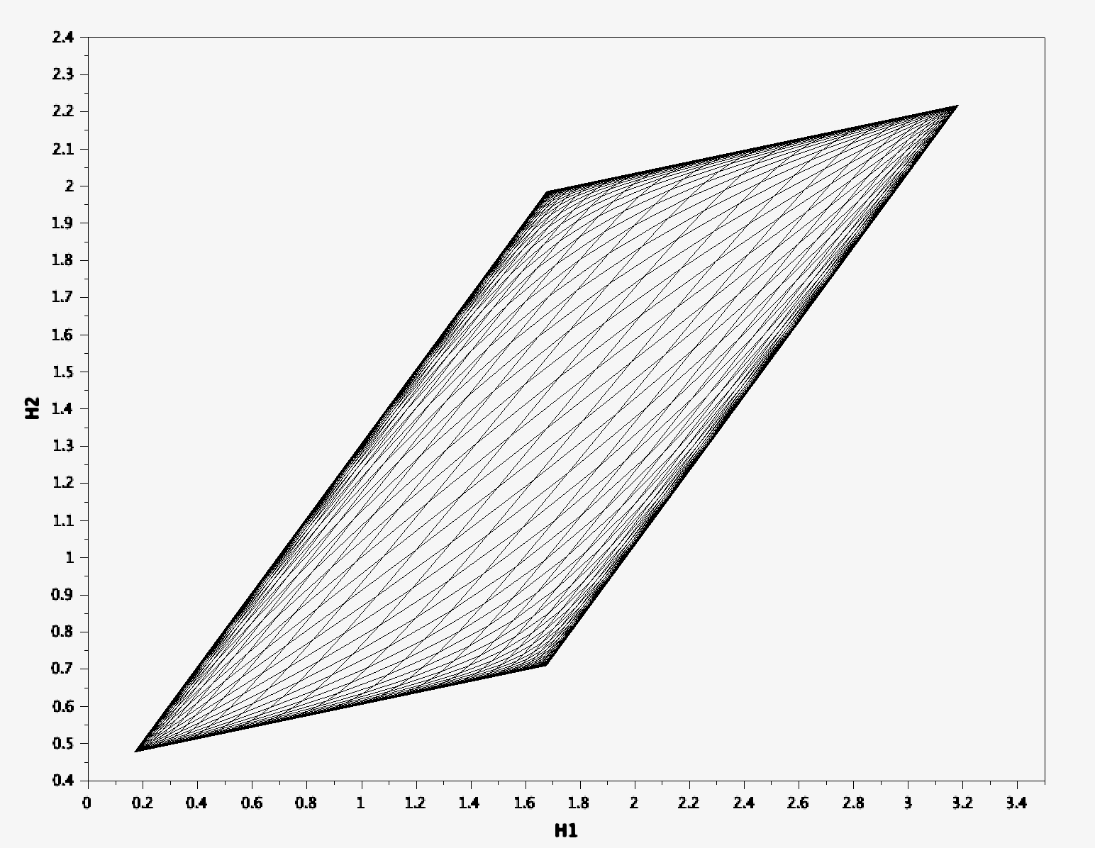
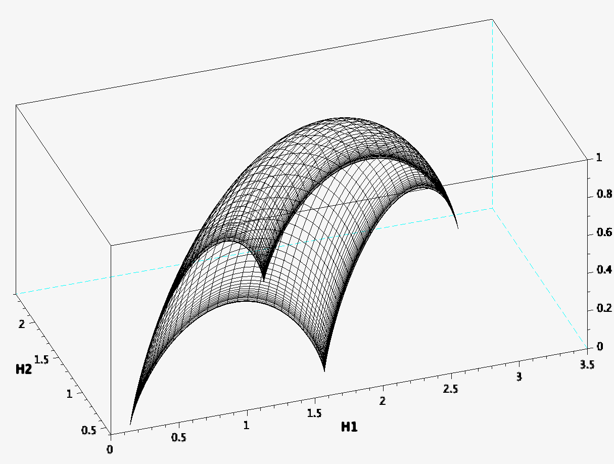
Figure 1. Case $0<p_{1},p_{2}<1/2$ or $1/2<p_{1},p_{2}<1$: Left: Support of $D_{{\mu_{p_{1}}},\nu_{\eta}}$. Right: Bivariate multifractal spectrum $D_{{\mu_{p_{1}}},\nu_{\eta}}$ of $(\mu_{p_{1}},\nu_{\eta})$.

Next, let us introduce for $q_{1},q_{2},H\in\mathbb{R}$ and $\eta\in[0,1]$ the following quantities:

$$T(q_{1},q_{2}) = -\log_{2}(p_{1}^{q_{1}}p_{2}^{q_{2}}+(1-p_{1})^{q_{1}}(1-p_{2})^{q_{2}})$$

$$T^{\eta}(q_{1},q_{2}) = \eta\tau_{\mu_{p_{1}}}(q_{1}+q_{2})+(1-\eta)T(q_{1},q_{2})$$

$$\widetilde{T}^{\eta}(q_{1},q_{2}) = -q_{1}\log_{2}(1-p_{1})-q_{2}(\eta\log_{2}p_{1}+(1-\eta)\log_{2}p_{2}).$$

Our second theorem deals with the case where the two parameters $(p_{1},p_{2})$ are both greater or both larger than 1/2.

Theorem 1.3.

Let $0<p_{1},p_{2}<1/2$ or $1/2<p_{1},p_{2}<1$. Let $\eta\in[0,1]$, and consider the pair of measures $(\mu_{p_{1}},\nu_{\eta})$. With probability one:

1. The bivariate $L^{q}$-spectrum of $(\mu_{p_{1}},\nu_{\eta})$ is $\tau_{\mu_{p_{1}},\nu_{\eta}}=T^{\eta}$.

2. The pair $(\mu_{p_{1}},\nu_{\eta})$ satisfies the bivariate multifractal formalism everywhere on their common support, which is a deterministic parallelogram $\mathcal{P}_{\eta}$.

Theorem 1.3 extends the results of [19, 1] which correspond to $\eta=0$. Calling

(9) $$\delta_{1,2} = \frac{-\log_{2}(p_{2})+\log_{2}(1-p_{2})}{-\log_{2}(p_{1})+\log_{2}(1-p_{1})},$$

we will see that the support of $D_{\mu_{p_{1}},\nu_{\eta}}$ is the parallelogram $\mathcal{P}_{\eta}$ generated by four straight lines, those with slopes $1$ or $\delta_{1,2}$ passing by the points $(H_{1,\min},\eta H_{1,\min}+(1-\eta)H_{2,\min})$ or $(H_{1,\max},H_{1,\max}+(1-\eta)H_{2,\max})$, see Section 5 for details, and Figure 1 for the graphs of $D_{\mu_{p_{1}},\nu_{\eta}}$ and $\tau^{*}_{\mu_{p_{1}},\nu_{\eta}}$.

The case where $(p_{1},p_{2})$ are not on the same side of 1/2 is much more delicate. Observe that $\delta_{1,2}>0$ when $p_{1}$ and $p_{2}$ are on the same side of $1/2$, while $\delta_{1,2}<0$ otherwise.

Theorem 1.4.

Let $0<p_{1}<1/2<p_{2}<1/2$. Let $\eta\in[0,1]$, and consider the pair of measures $(\mu_{p_{1}},\nu_{\eta})$.

With probability one:

1. The bivariate $L^{q}$-spectrum of $(\mu_{p_{1}},\nu_{\eta})$ is $\tau_{\mu_{p_{1}},\nu_{\eta}}=\min(T^{\eta},\widetilde{T}^{\eta})$, and the support of $\tau_{\mu_{p_{1}},\nu_{\eta}}^{*}$ is is a deterministic pentagon $\mathcal{P}^{\eta}_{1}$.

2. The support of the bivariate multifractal spectrum $D_{\mu_{p_{1}},\nu_{\eta}}$ is a deterministic pentagon $\mathcal{P}^{\eta}_{2}$ which is strictly larger than $\mathcal{P}^{\eta}_{1}$ when $\eta\neq 0$ or $\eta\neq 1$.

The values of $D_{\mu_{p_{1}},\nu_{\eta}}$ and the pentagons are given in Section 6, and are plotted in Figures 5, 4 and 2.

Besides the measures provided by Theorem 1.2, the pair $(\mu_{p_{1}},\nu_{\eta})$ is to our knowledge the first example of pair of measures for which the supports of $D_{\mu_{p_{1}},\nu_{\eta}}$ and $(\tau_{\mu_{p_{1}},\nu_{\eta}})^{*}$ are proved not to coincide. The proportion between the area of $\mathcal{P}^{\eta}_{1}$ and $\mathcal{P}^{\eta}_{2}\setminus\mathcal{P}^{\eta}_{1}$ depends on the parameter $\eta$, and somehow characterizes the correlation between $\mu_{p_{1}}$ and $\nu_{\eta}$.

Corollary 1.5.

The pair $(\mu_{p_{1}},\nu_{\eta})$ does not satisfy the bivariate multifractal formalism everywhere.

The fact that the bivariate multifractal formalism does not hold is immediate as soon as the supports of $\tau_{\mu_{p_{1}},\nu_{\eta}}^{*}$ and $D_{\mu_{p_{1}},\nu_{\eta}}$ do not coincide. Here, the two spectra do not even coincide on a large part of $\mathcal{P}^{\eta}_{1}$ (which is the intersection of the supports), again depending on $\eta$, see Section 6 for some discussions. The pictures plotted in Figure 2 show that the two spectra have distinct shapes, even if they coincide on some region of the plane. More precisely:

• The shape of the Legendre spectrum $\tau_{\mu_{p_{1}},\nu_{\eta}}^{*}$ is quite easily understandable, remembering that $\tau_{\mu_{p_{1}},\nu_{\eta}}=\min(T^{\eta},\widetilde{T}^{\eta})$. Indeed, $\tau_{\mu_{p_{1}},\nu_{\eta}}^{*}$ is composed in one region of a smooth part $(T^{\eta})^{*}$ (like in the case where $p_{1}$ and $p_{2}$ are located on the same side of $1/2$), and in a second region of a cone with center $(H_{1,\min},\eta H_{1,\max}+(1-\eta)H_{2,\min})$ and tangent to $(T^{\eta})^{*}$.

• The shape of $D_{\mu_{p_{1}},\nu_{\eta}}$ results from various constraints on the possible simultaneous behaviors of $\mu_{p_{1}}$ and $\nu_{\eta}$ at a given point $t\in[0,1]$. It is worth noticing that many possible pairs $(H_{1},H_{2})$ are not seen by the Legendre spectrum, since $\mathcal{P}^{\eta}_{1}$ is strictly smaller than $\mathcal{P}^{\eta}_{2}$.

• The bivariate spectrum $D_{\mu_{p_{1}},\nu_{\eta}}$ lies above the Legendre spectrum $\tau_{\mu_{p_{1}},\nu_{\eta}}^{*}$ on a large part of $\mathcal{P}^{\eta}_{1}$, so investigating the region where the multifractal formalism holds is not key here.

The main reason justifying these differences is that for a given $t\in[0,1]$, it may happen that the liminf local dimensions $\underline{\dim}({\mu_{p_{1}}},x)$ and $\underline{\dim}(\nu_{\eta},x)$ may reached at different scales, in the sense that $\displaystyle\frac{\log\mu_{p_{1}}(B(t,r))}{\log r}\sim\underline{\dim}({\mu_{p_{1}}},x)$ and $\displaystyle\frac{\log\nu_{\eta}(B(t,r^{\prime}))}{\log r^{\prime}}\sim\underline{\dim}(\nu_{\eta},x)$ at very different radii $r$ and $r^{\prime}$ (this does not happen when considering limit local dimensions). Then, since the computation of $\tau_{\mu_{p_{1}},\nu_{\eta}}$ (5) only involves the measures of dyadic intervals at the same scale $2^{-j}$, the possible non-simultaneity implies that $\tau_{\mu_{p_{1}},\nu_{\eta}}$ cannot catch all possible behaviors. Describing and quantifying this variety of behaviors is the main issue in the following and in the computations.

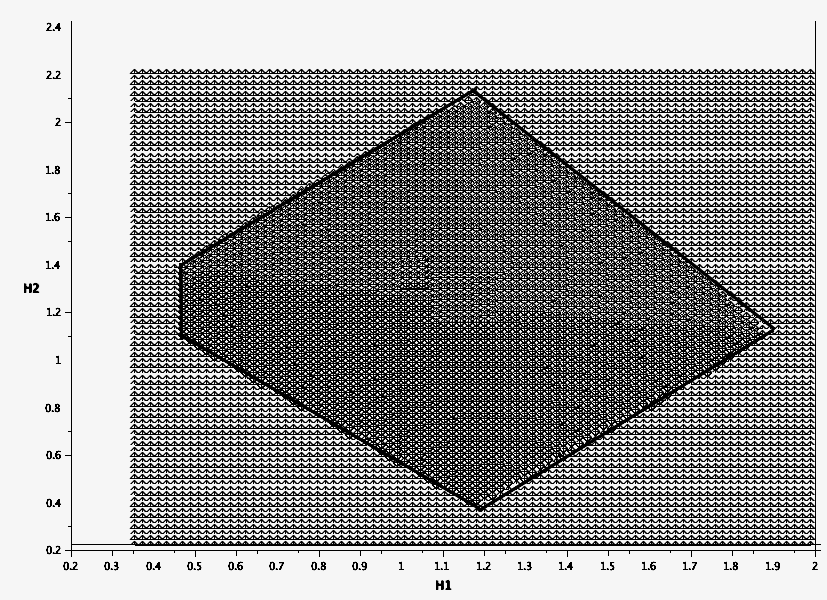
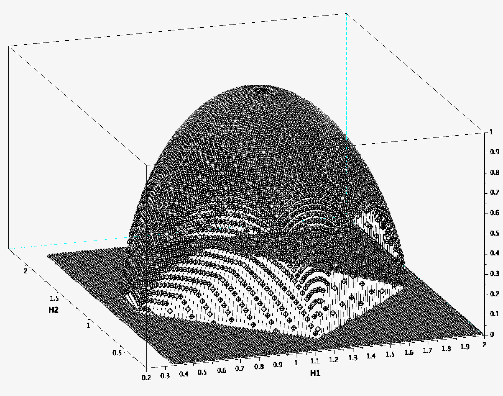
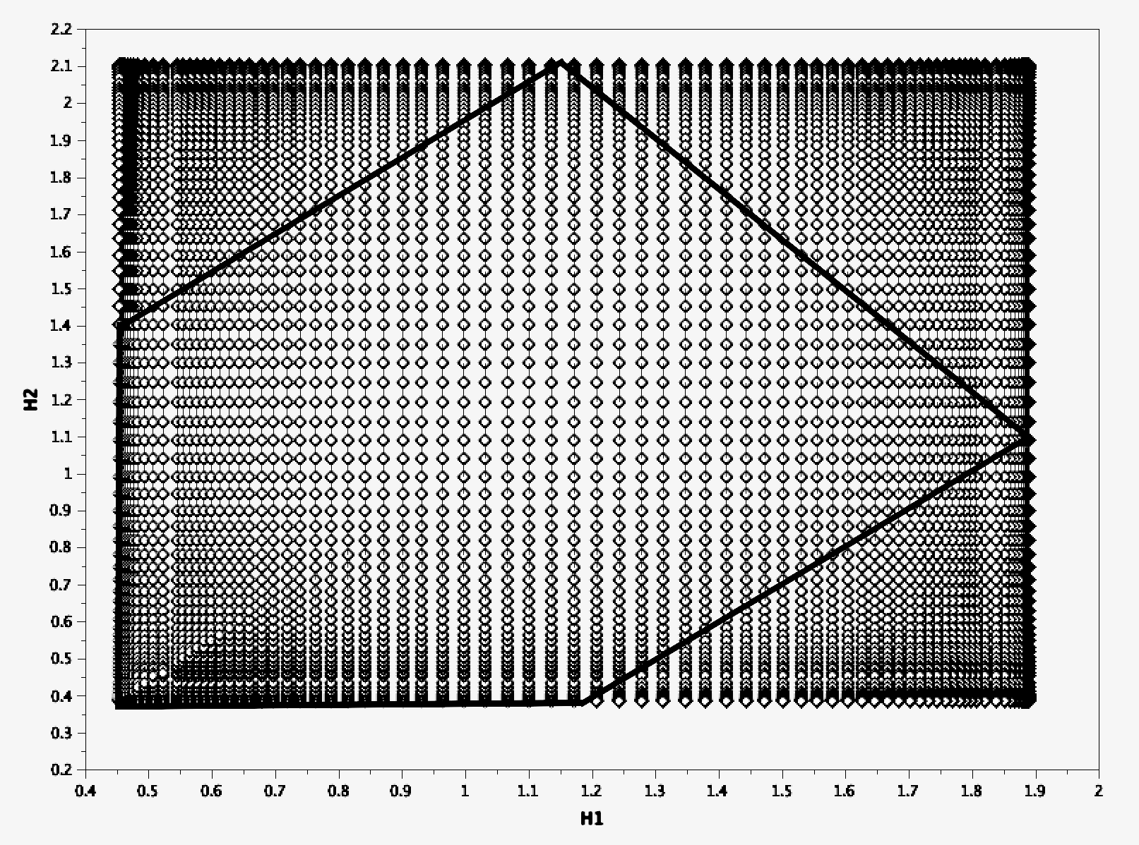
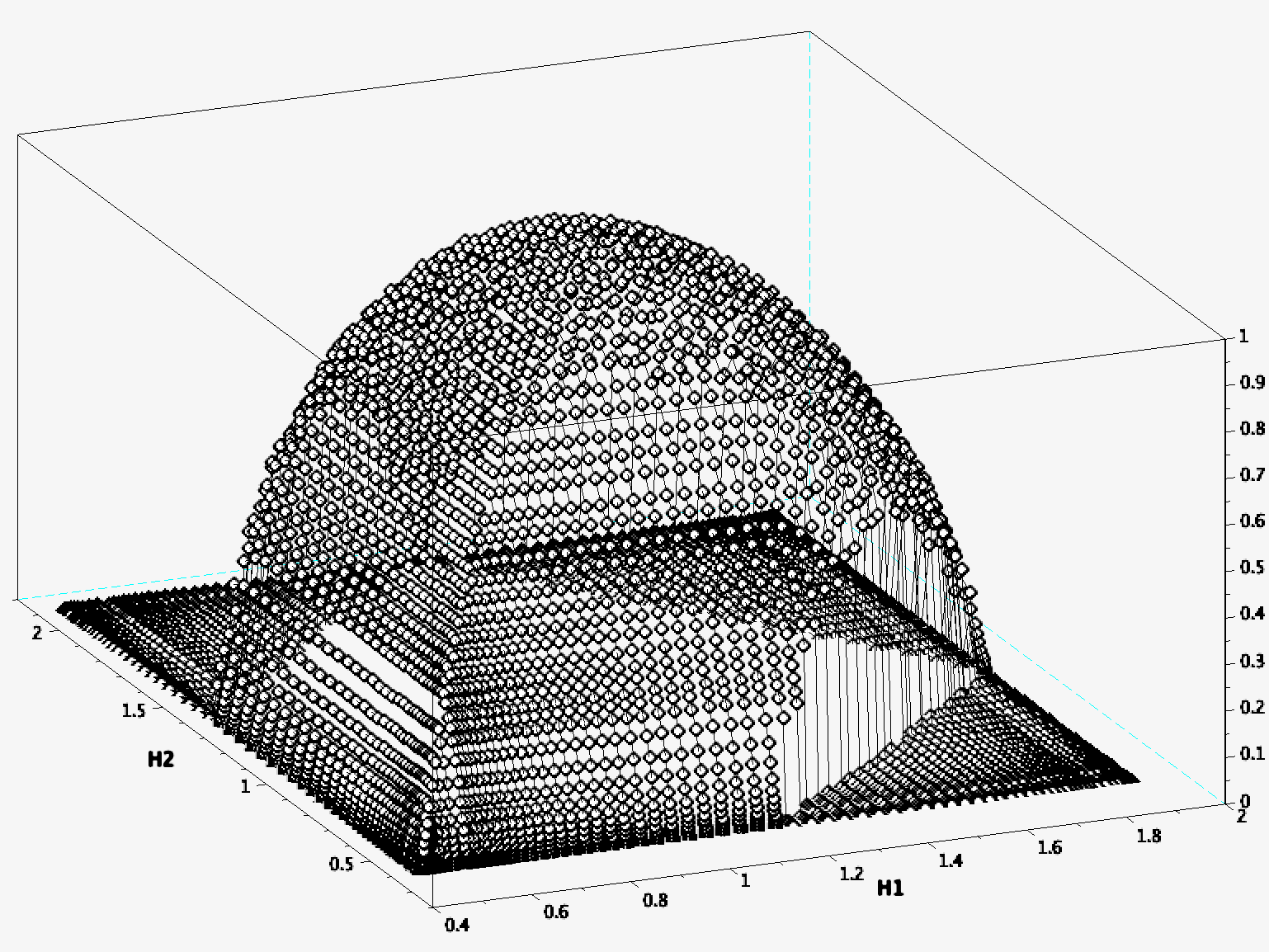
Figure 2. Case $0<p_{1}=0.27<1/2<p_{2}=0.8$ and $\eta=0.5$. Top left: Support of the Legendre spectrum $\tau_{{\mu_{p_{1}}},\nu_{\eta}}^{*}$ Top right: Legendre spectrum $\tau_{{\mu_{p_{1}}},\nu_{\eta}}^{*}$. Bottom left: Support of the multifractal spectrum $D_{{\mu_{p_{1}}},\nu_{\eta}}$ Bottom right: Bivariate multifractal spectrum $D_{{\mu_{p_{1}}},\nu_{\eta}}$. The supports are distinct (but not disjoint) pentagons.

The article is organized as follows. In Section 2, we set up the notations, and prove Theorem 1.2. Next, in Section 3, we recall useful facts on Bernoulli measures, and prove additional ones. Section 4 contains preliminary results useful for the rest of the article. Theorem 1.3 is proved in Section 5. Finally, Theorem 1.4, which is much more delicate, is obtained in Section 6. A subtle joint analysis of the possible simultaneous behaviors of ${\mu_{p_{1}}}(I)$ and $\nu_{\eta}(I)$, for all dyadic intervals $I$, is necessary.

Let us conclude by underlining the richness of such analyses, and the necessity to enrich the classes of objects for which the multivariate multifractal analysis be performed.

2. Some notations and proof of Theorem 1.2

2.1. Notations

We adopt the convention that for $a,b\in\mathbb{R}$, $[a,b]$ stands for the interval $[\min(a,b),\max(a,b)]$, and that $0^{q}=0$, for every $q\in\mathbb{R}$.

For every $j\geq 1$, let $\Sigma_{j}=(\{0,1\})^{j}$ be the set of words of length $j$ on the alphabet $\{0,1\}$, and $\Sigma=(\{0,1\})^{\mathbb{N}}$ and $\Sigma^{*}=\bigcup_{j\geq 0}\Sigma_{j}$ be respectively the sets of infinite and finite words. The length of $w\in\Sigma^{*}$ is denoted by $|w|$, and $|w|=\infty$ when $w\in\Sigma$. When $w\in\Sigma^{*}$, we usually write $w=w_{1}\cdots w_{|w|}$ and $w\in\Sigma_{|w|}$, and $w=w_{1}\cdots w_{n}\cdots$ when $w\in\Sigma$. Then if $j\leq|w|$, $w_{|j}$ is the prefix of $w$ of length $j$. When $w\in\Sigma^{*}$, the cylinder $\lfloor w\rfloor$ is the set of words $w^{\prime}\in\Sigma\cup\Sigma^{*}$ whose prefix of length $|w|$ equals $w$.

The concatenation of two words $w\in\Sigma^{*}$ and $w^{\prime}\in\Sigma^{*}\cup\Sigma$ is denoted by $ww^{\prime}$.

We define for $w\in\Sigma^{*}\cup\Sigma$

(10) $$x_{w}=\sum_{\ell=1}^{|w|}w_{\ell}2^{-\ell}\in[0,1]$$

and every real number $x\in[0,1]$ can be written $x=x_{w}$ for some $w\in\Sigma^{*}\cup\Sigma$, the decomposition being unique except for dyadic numbers $x_{w}$ for $w\in\Sigma^{*}$.

The dyadic intervals are encoded using words $w\in\Sigma_{j}$ by

$$I_{w}=\Big{[}\sum_{\ell=1}^{j}w_{\ell}2^{-\ell},2^{-j}+\sum_{\ell=1}^{j}w_{\ell}2^{-\ell}\Big{]},$$

and we will talk indifferently about $I_{w}$ or the cylinder $\lfloor w\rfloor$, and write $I\in\Sigma_{j}$ or $I\in\mathcal{D}_{j}$ depending on the context.

For every interval $I\in\mathcal{D}_{j}$, we write

$$I^{+}=I+2^{-j}\ \ \mbox{ and }\ \ I^{-}=I-2^{-j}.$$

For every $x\in[0,1]$, call $I_{j}(x)$ the unique dyadic interval of $\Sigma_{j}$ containing $x$, $I_{j}^{+}(x)=I_{j}(x)+2^{-j}$, $I_{j}^{-}(x)=I_{j}(x)-2^{-j}$, and ${I}^{(n)}_{j}(x)=I_{j}(x)\cup I_{j}^{+}(x)\cup I_{j}^{-}(x)$.

For an interval $I=[a,b]$ and ${\varepsilon}>0$, we use the notation

$$I\pm{\varepsilon}=I+[-{\varepsilon},+{\varepsilon}]=[a-{\varepsilon},b+{\varepsilon}].$$

Finally, the dimension of a Borel probability measure $\mu$ is

$$\dim(\mu)=\inf\{\dim_{H}(A):\mu(A)=1\}.$$

2.2. Proof of Theorem 1.2

We are going to build two Borel probability measures $\nu_{1}$ and $\nu_{2}$ such that $\mbox{Supp}(D_{\nu_{1},\nu_{2}})=\{(1/2,1/2),(1/2,+\infty),(+\infty,1/2),(+\infty,+\infty)\}$, while $\mbox{Supp}(\tau^{*}_{\nu_{1},\nu_{2}})$ is the triangle with edges $(1,1/2),(1/2,1),(1,1)$. In particular, the two supports do not intersect.

For this, we will alternate between two simple construction schemes:

• Starting from a dyadic interval $I\in\Sigma_{2j}$ with positive $\nu_{i}$-mass, the $\nu_{i}$-mass of every $J\in\Sigma_{2(j+1)}$ with $J\subset I$ is put to $\nu(I)/4$.

• Starting from a dyadic interval $I\in\Sigma_{2j}$ with positive $\nu_{i}$-mass, the $\nu_{i}$-mass of the first and the last of the four subintervals $J\in\Sigma_{2(j+1)}$ with $J\subset I$ is put to $\nu(I)/2$, and the mass of the two others is put to 0.

The first one mimics the Lebesgue measure, while the second one is an intermediary step leading to a Cantor set.

Let $({\varepsilon}_{n}:=2^{-(n+2)})_{n\geq 1}$, and $(j^{i}_{n})_{n\geq 1}$, for $i=1,...,4$, be four sequences of integers tending fast to infinity, whose values will be given inductively along the construction.

Start with $\nu_{1}([0,1])=\nu_{2}([0,1])=1$. Let us assume that at generation $2j^{4}_{n}$, for $i\in\{1,2\}$, for every $I\in\Sigma_{2j_{4}^{n}}$, when $\nu_{i}(I)\neq 0$, $\nu_{i}(I)$ depends only on $i$ and

(11) $$2^{-2j_{4}^{n}(1+{\varepsilon}_{n})}=|I|^{1+{\varepsilon}_{n}}\leq\nu_{i}(I)\leq|I|^{1-{\varepsilon}_{n}}=2^{-2j_{4}^{n}(1-{\varepsilon}_{n})}.$$

In particular, the measures $\nu_{i}$ are ”doubling at scale $2^{-2j_{4}^{n}}$”, i.e. for every $I\in\Sigma_{2j_{4}^{n}}$ with $\nu(I)>0$, $\nu(I)\leq\nu(3I)\leq 3\nu(I)$. This implies that the two sums $\sum_{I\in\Sigma_{2j^{4}_{n}}}\nu_{1}(I)^{q_{1}}\nu_{2}(I)^{q_{2}}$ and $\sum_{I\in\Sigma_{2j^{4}_{n}}}\nu_{1}(3I)^{q_{1}}\nu_{2}(3I)^{q_{2}}$ are equivalent up to universal constants, and we shall compute $\tau_{\nu_{1},\nu_{2}}$ in this section by replacing $3I$ in formula (5) by $I$.

Assume also that

(12) $$2^{2j^{4}_{n}(1-2{\varepsilon}_{n})}\leq\#\{I\in\Sigma_{2j^{4}_{n}}:\nu_{1}(I)\nu_{2}(I)\neq 0\}\leq 2^{2j^{4}_{n}(1+2{\varepsilon}_{n})}.$$

For $q\in\mathbb{R}$, let us write $\mbox{sgn}(q)=+1$ when $q\geq 0$ and $\mbox{sgn}(q)=-1$ when $q<0$. The previous inequalities yield

$$\sum_{I\in\Sigma_{2j^{4}_{n}}}\nu_{1}(I)^{q_{1}}\nu_{2}(I)^{q_{2}} \geq 2^{2j^{4}_{n}(1-2{\varepsilon}_{n})}2^{-2j_{4}^{n}(1+\mbox{\tiny sgn}(q_{1}){\varepsilon}_{n})q_{1}}2^{-2j_{4}^{n}(1+\mbox{\tiny sgn}(q_{2}){\varepsilon}_{n})q_{2}}$$

$$\sum_{I\in\Sigma_{2j^{4}_{n}}}\nu_{1}(I)^{q_{1}}\nu_{2}(I)^{q_{2}} \leq 2^{2j^{4}_{n}(1+2{\varepsilon}_{n})}2^{-2j_{4}^{n}(1-\mbox{\tiny sgn}(q_{1}){\varepsilon}_{n})q_{1}}2^{-2j_{4}^{n}(1-\mbox{\tiny sgn}(q_{2}){\varepsilon}_{n})q_{2}}.$$

Hence,

(13) $$|\tau_{\nu_{1},\nu_{2},2j^{4}_{n}}(q_{1},q_{2})-(q_{1}+q_{2}-1)|\leq(|q_{1}|+|q_{2}|+2){\varepsilon}_{n}.$$

These conditions are satisfied at generation $j^{1}_{0}=j^{2}_{0}=j^{3}_{0}=j^{4}_{0}=0$. Next, we proceed iteratively using 4 consecutive steps:

Step 1: As long as $j^{4}_{n}\leq j\leq j^{1}_{n+1}-1$, the two measures are constructed simultaneously on $\Sigma_{2j}$ by iterating scheme (P1) for $\nu_{1}$ and (P2) for $\nu_{2}$. More precisely, for every $I\in\Sigma_{2j}$ such that $\nu_{1}(I)>0$, apply (P1) to define $\nu_{1}$ on the intervals of $\Sigma_{2(j+1)}$, and similarly for every $I\in\Sigma_{2j}$ such that $\nu_{2}(I)>0$, apply (P2) to define $\nu_{2}$ on the intervals of $\Sigma_{2(j+1)}$.

Let us choose $j_{n+1}^{1}$ as the smallest integer such that $\frac{5j^{4}_{n}+1}{j^{1}_{n+1}}\leq{\varepsilon}_{n+1}/2$.

At the last step, at generation $2j_{1}^{n+1}$:

• for every $I\in\Sigma_{2j_{n+1}^{1}}$, either $\nu_{1}(I)=0$ or $\nu_{1}(I)=\nu_{1}(J)2^{-2(j_{n+1}^{1}-j^{4}_{n})}$. Our choice for $j^{1}_{n+1}$ and (11) give that

  (14) $$2^{-2j_{n+1}^{1}(1+{\varepsilon}_{n+1})} \leq 2^{-2j_{4}^{n}(1+{\varepsilon}_{n})}2^{-2(j_{n+1}^{1}-j^{4}_{n})}\leq\nu_{1}(I)$$

  $$\leq 2^{-2j_{4}^{n}(1-{\varepsilon}_{n})}2^{-2(j_{n+1}^{1}-j^{4}_{n})}\leq 2^{-2j_{n+1}^{1}(1-{\varepsilon}_{n+1})}.$$

  Also, for every $j\in\{2j^{4}_{n},...,2j^{1}_{n+1}\}$ and $I\in\Sigma_{j}$,

  (15) $$2^{-j(1+{\varepsilon}_{n})}\leq\nu_{1}(I)\leq 2^{-j(1-{\varepsilon}_{n})}.$$

• for every $I\in\Sigma_{2j_{n+1}^{1}}$, either $\nu_{2}(I)=0$ or $\nu_{2}(I)=\nu_{2}(J)2^{-(j_{n+1}^{1}-j^{4}_{n})}$. Then

  (16) $$2^{-j_{n+1}^{1}(1+{\varepsilon}_{n+1})} \leq 2^{-2j_{4}^{n}(1+{\varepsilon}_{n})}2^{-(j_{n+1}^{1}-j^{4}_{n})}\leq\nu_{2}(I)$$

  $$\leq 2^{-2j_{4}^{n}(1-{\varepsilon}_{n})}2^{-(j_{n+1}^{1}-j^{4}_{n})}\leq 2^{-j_{n+1}^{1}(1-{\varepsilon}_{n+1})}.$$

  Also, for every $j\in\{2j^{4}_{n},...,2j^{1}_{n+1}\}$ and $I\in\Sigma_{j}$,

  (17) $$2^{-j(1+{\varepsilon}_{n})}\leq\nu_{2}(I)\leq 2^{-j/2(1-{\varepsilon}_{n})}.$$

Intuitively, at an interval $I$ of generation $2j_{n+1}^{1}$ such that $\nu_{1}(I)\nu_{2}(I)\neq 0$, one has $\nu_{1}(I)\sim|I|$ while $\nu_{2}(I)\sim|I|^{1/2}$.

Observe that by the scheme (P2) and by (12),

(18) $$2^{j^{1}_{n+1}(1-{\varepsilon}_{n+1})}\leq 2^{j^{1}_{n+1}-j^{4}_{n}}2^{2j^{4}_{n}(1-2{\varepsilon}_{n})} \leq\#\{I\in\Sigma_{2j^{1}_{n+1}}:\nu_{1}(I)\nu_{2}(I)\neq 0\}$$

$$\leq 2^{j^{1}_{n+1}-j^{4}_{n}}2^{2j^{4}_{n}(1+2{\varepsilon}_{n})}\leq 2^{j^{1}_{n+1}(1+{\varepsilon}_{n+1})}.$$

So, even if there are intervals $I$ such that $\nu_{1}(I)\neq 0$ and $\nu_{2}(I)=0$ (or the opposite situation), they are heuristically not the most numerous ones.

Similar computations as in the preliminary step give

$$\sum_{I\in\Sigma_{2j^{1}_{n+1}}}\nu_{1}(I)^{q_{1}}\nu_{2}(I)^{q_{2}} \geq 2^{j^{1}_{n+1}(1-{\varepsilon}_{n+1})}2^{-2j^{1}_{n+1}(1+\mbox{\tiny sgn}(q_{1}){\varepsilon}_{n+1})q_{1}}2^{-j_{1}^{n+1}(1+\mbox{\tiny sgn}(q_{2}){\varepsilon}_{n+1})q_{2}}$$

$$\sum_{I\in\Sigma_{2j^{1}_{n+1}}}\nu_{1}(I)^{q_{1}}\nu_{2}(I)^{q_{2}} \leq 2^{j^{1}_{n+1}(1+{\varepsilon}_{n+1})}2^{-2j^{1}_{n+1}(1-\mbox{\tiny sgn}(q_{1}){\varepsilon}_{n+1})q_{1}}2^{-j_{1}^{n+1}(1-\mbox{\tiny sgn}(q_{2}){\varepsilon}_{n+1})q_{2}}.$$

Hence,

(19) $$|\tau_{\nu_{1},\nu_{2},2j^{1}_{n+1}}(q_{1},q_{2})-(q_{1}+q_{2}/2-1/2)|\leq(|q_{1}|+|q_{2}|+2){\varepsilon}_{n+1}.$$

Also, for every $j\in\{2j^{4}_{n},...,2j^{1}_{n+1}\}$,

$$\tau_{\nu_{1},\nu_{2},j}(q_{1},q_{2})\in[q_{1}+q_{2}/2-1/2,q_{1}+q_{2}-1]\pm(|q_{1}|+|q_{2}|+2){\varepsilon}_{n},$$

recalling that $[a,b]$ stands for the interval $[\min(a,b),\max(a,b)]$.

Step 2: Next we iterate the same scheme (P1) for $\nu_{1}$ and $\nu_{2}$ until generation $2j^{2}_{n+1}$ as follows: for every $j\in\{j^{1}_{n+1},...,j^{2}_{n+1}-1\}$, for every $I\in\Sigma_{2j}$ such that $\nu_{i}(I)>0$ ($i\in\{1,2\}$), apply (P1) to define $\nu_{i}$ on the intervals of $\Sigma_{2(j+1)}$. Again, at every generation $j\leq 2j^{2}_{n+1}$, the value of $\nu_{i}(I)$ (when $\nu_{i}(I)>0$) for $I\in\Sigma_{j}$ depends on $j$ only.

Set $j_{n+1}^{2}$ as the smallest integer such that $\frac{5j^{1}_{n+1}}{j^{2}_{n+1}}\leq{\varepsilon}_{n+1}/2$.

At generation $2j^{2}_{n+1}$, one has

• for every $I\in\Sigma_{2j_{n+1}^{2}}$, either $\nu_{1}(I)=0$ or $\nu_{1}(I)=\nu_{1}(J)2^{-2(j_{n+1}^{2}-j_{n+1}^{1})}$. Then (14) yields

  (20) $$2^{-2j_{n+1}^{2}(1+{\varepsilon}_{n+1})} \leq 2^{-2j_{n+1}^{1}(1+{\varepsilon}_{n+1})}2^{-2(j_{n+1}^{2}-j_{n+1}^{1})}\leq\nu_{1}(I)$$

  $$\leq 2^{-2j_{n+1}^{1}(1-{\varepsilon}_{n+1})}2^{-2(j_{n+1}^{2}-j_{n+1}^{1})}\leq 2^{-2j_{n+1}^{2}(1-{\varepsilon}_{n+1})}.$$

  Also, for every $j\in\{2j^{1}_{n+1},...,2j_{n+1}^{2}\}$ and $I\in\Sigma_{j}$,

  (21) $$2^{-j(1+{\varepsilon}_{n})}\leq\nu_{1}(I)\leq 2^{-j(1-{\varepsilon}_{n})}.$$

• for every $I\in\Sigma_{2j_{n+1}^{2}}$, either $\nu_{2}(I)=0$ or $\nu_{2}(I)=\nu_{2}(J)2^{-2(j_{n+1}^{2}-j_{n+1}^{1})}$. Then

  (22) $$2^{-2j_{n+1}^{2}(1+{\varepsilon}_{n+1})} \leq 2^{-2j_{n+1}^{1}(1+{\varepsilon}_{n+1})}2^{-2(j_{n+1}^{2}-j_{n+1}^{1})}\leq\nu_{2}(I)$$

  $$\leq 2^{-2j_{n+1}^{1}(1-{\varepsilon}_{n+1})}2^{-2(j_{n+1}^{2}-j_{n+1}^{1})}\leq 2^{-2j_{n+1}^{2}(1-{\varepsilon}_{n+1})}.$$

  Also, for every $j\in\{2j^{1}_{n+1},...,2j^{2}_{n+1}\}$ and $I\in\Sigma_{j}$,

  (23) $$2^{-j(1+{\varepsilon}_{n})}\leq\nu_{2}(I)\leq 2^{-j/2(1-{\varepsilon}_{n})}.$$

Intuitively, at an interval $I$ of generation $j_{n+1}^{2}$, one has $\nu_{i}(I)\sim|I|$ for $i\in\{1,2\}$.

The same observations as in Step 1 give

(24) $$2^{2j_{n+1}^{2}(1-{\varepsilon}_{n+1})}=2^{2(j_{n+1}^{2}-j^{1}_{n+1})}2^{j_{n+1}^{1}(1-2{\varepsilon}_{n})} \leq\#\{I\in\Sigma_{2j^{2}_{n+1}}:\nu_{1}(I)\nu_{2}(I)\neq 0\}$$

$$\leq 2^{2(j_{n+1}^{2}-j^{1}_{n+1})}2^{2j_{n+1}^{1}(1+2{\varepsilon}_{n})}\leq 2^{2j_{n+1}^{2}(1+{\varepsilon}_{n+1})}.$$

and

$$\sum_{I\in\Sigma_{2j_{n+1}^{2}}}\nu_{1}(I)^{q_{1}}\nu_{2}(I)^{q_{2}} \geq 2^{2j_{n+1}^{2}(1-{\varepsilon}_{n+1})}2^{-2j_{n+1}^{2}(1+\mbox{\tiny sgn}(q_{1}){\varepsilon}_{n+1})q_{1}}2^{-j_{n+1}^{2}(1+\mbox{\tiny sgn}(q_{2}){\varepsilon}_{n}+1)q_{2}}$$

$$\sum_{I\in\Sigma_{2j^{2}_{n+1}}}\nu_{1}(I)^{q_{1}}\nu_{2}(I)^{q_{2}} \leq 2^{2j_{n+1}^{2}(1+{\varepsilon}_{n+1})}2^{-2j_{n+1}^{2}(1-\mbox{\tiny sgn}(q_{1}){\varepsilon}_{n+1})q_{1}}2^{-j_{n+1}^{2}(1-\mbox{\tiny sgn}(q_{2}){\varepsilon}_{n}+1)q_{2}}.$$

Hence,

(25) $$|\tau_{\nu_{1},\nu_{2},2j_{n+1}^{2}}(q_{1},q_{2})-(q_{1}+q_{2}-1)|\leq(|q_{1}|+|q_{2}|+2){\varepsilon}_{n+1}.$$

Also, for every $j\in\{2j^{1}_{n+1},...,2j_{n+1}^{2}\}$ and $I\in\Sigma_{j}$,

$$\tau_{\nu_{1},\nu_{2},j}(q_{1},q_{2})\in[q_{1}+q_{2}/2-1/2,q_{1}+q_{2}-1]\pm(|q_{1}|+|q_{2}|+2){\varepsilon}_{n}$$

Step 3: Observe that we are back to the situation before applying Step 1. Next, one proceeds as in Step 1, except that we apply (P2) to $\nu_{1}$ and (P1) to $\nu_{2}$. The computations are the same, except that the roles of $\nu_{1}$ and $\nu_{2}$ are switched.

The same lines of computations give for $j^{3}_{n+1}$ large enough:

• for every $I\in\Sigma_{2j_{n+1}^{3}}$, either $\nu_{1}(I)=0$ or

  (26) $$2^{-j_{n+1}^{3}(1+{\varepsilon}_{n+1})} \leq\nu_{1}(I)2^{-j_{n+1}^{3}(1-{\varepsilon}_{n+1})}.$$

  For every $j\in\{2j^{2}_{n+1},...,2j^{3}_{n+1}\}$,

  (27) $$2^{-j/2(1+{\varepsilon}_{n})}\leq\nu_{1}(I)\leq 2^{-j(1-{\varepsilon}_{n})}.$$

• for every $I\in\Sigma_{2j_{n+1}^{3}}$, either $\nu_{2}(I)=0$ or

  (28) $$2^{-j_{n+1}^{3}(1+{\varepsilon}_{n+1})} \leq\nu_{2}(I)\leq 2^{-j_{n+1}^{3}(1-{\varepsilon}_{n+1})}.$$

  For every $j\in\{2j^{2}_{n+1},...,2j^{3}_{n+1}\}$,

  (29) $$2^{-j(1+{\varepsilon}_{n})}\leq\nu_{2}(I)\leq 2^{-j/2(1-{\varepsilon}_{n})}.$$

• One has

  (30) $$2^{j^{3}_{n+1}(1-{\varepsilon}_{n+1})}\leq\#\{I\in\Sigma_{2j^{3}_{n+1}}:\nu_{1}(I)\nu_{2}(I)\neq 0\}\leq 2^{j^{3}_{n+1}(1+{\varepsilon}_{n+1})}.$$

• One has

  (31) $$|\tau_{\nu_{1},\nu_{2},2j^{3}_{n+1}}(q_{1},q_{2})-(q_{1}/2+q_{2}-1/2)|\leq(|q_{1}|+|q_{2}|+2){\varepsilon}_{n+1}.$$

• For every $j\in\{2j^{2}_{n+1},...,2j^{3}_{n+1}\}$,

  $$\tau_{\nu_{1},\nu_{2},j}(q_{1},q_{2})\in[q_{1}/2+q_{2}-1/2,q_{1}+q_{2}-1]\pm(|q_{1}|+|q_{2}|+2){\varepsilon}_{n}$$

Step 4: One applies (P1) to the two measures, and for a suitable choice of $j^{4}_{n+1}$, the estimates (20), (21), (22), (23), (24) and (25) hold at a generation $j^{4}_{n+1}$ chosen sufficiently large with respect to $j^{3}_{n+1}$.

Observe that after Step 4, we are back to the initial conditions (before applying Step 1). Hence the process can be iteratively applied and the two measures $\nu_{1}$ and $\nu_{2}$ are simultaneously constructed. Also, the two measures are by construction doubling on their support, i.e. for every $I\in\Sigma_{j}$ with $\nu(I)>0$, $\nu(3I)\leq 3\nu(I)$.

One now collects the information:

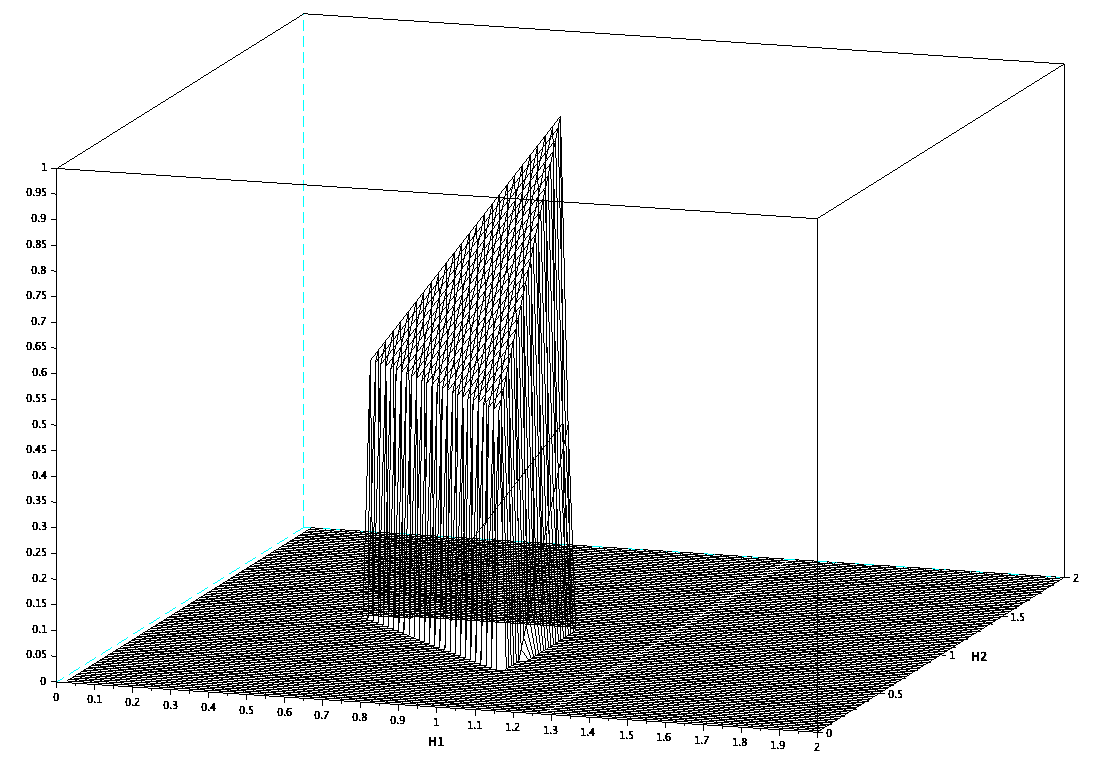
Figure 3. Legendre transform of $\tau_{\nu_{1},\nu_{2}}$.

• Let $i\in\{1,2\}$, ${\varepsilon}>0$, and $x\in\mathrm{supp}(\nu_{i})$. By construction, (16) and (28), there exist infinitely many generations $j=2j^{1}_{n}$ ot $j=2j^{3}_{n}$ such that ${\varepsilon}_{n}\leq{\varepsilon}$, $2^{-j/2(1+{\varepsilon})}\leq\nu_{i}(B(x,2^{-j}))=\nu_{i}(I_{j}(x))\leq 2^{-j/2(1-{\varepsilon})}$.

  Also, for every $j$ large, $2^{-j/2(1+{\varepsilon})}\leq\nu_{i}(B(x,2^{-j}))\leq 2^{-j(1-{\varepsilon})}$ by (15), (17), (21), (23) and the same bounds hold at Step 3 and 4. Hence $\underline{\dim}(\nu_{i},x)=1/2$.

• As a consequence of the first item, the bivariate multifractal spectrum of $(\nu_{1},\nu_{2})$ is:

  $$D_{\nu_{1},\nu_{2}}(H_{1},H_{2})=\begin{cases}\dim(\mathrm{supp}(\nu_{1})\cap\mathrm{supp}(\nu_{2}))&\mbox{ when }H_{1}=H_{2}=1/2\\ \dim(\mathrm{supp}(\nu_{1})\cap\mathrm{supp}(\nu_{2})^{c})&\mbox{ when }H_{1}=1/2,H_{2}=+\infty\\ \dim(\mathrm{supp}(\nu_{1})^{c}\cap\mathrm{supp}(\nu_{2}))&\mbox{ when }H_{1}=+\infty,H_{2}=1/2\\ \dim(\mathrm{supp}(\nu_{1})^{c}\cap\mathrm{supp}(\nu_{2})^{c})&\mbox{ when }H_{1}=H_{2}=+\infty.\end{cases}$$

  Even if it not necessary for our purpose, one can check that $\dim(\mathrm{supp}(\nu_{1})\cap\mathrm{supp}(\nu_{2}))=1/2$, $\dim(\mathrm{supp}(\nu_{1})^{c}\cap\mathrm{supp}(\nu_{2})^{c})=1$, $\dim(\mathrm{supp}(\nu_{i})\cap\mathrm{supp}(\nu_{j})^{c})=1/2$ for $i\neq j$.

• By (19), (25), (31) and (13) (which is also obtained after Step 4) and the inequalities that follow these equations, and recalling that ${\varepsilon}_{n}\to 0$ when $n$ tends to infinity, one deduces that

  $$\tau_{\nu_{1},\nu_{2}}(q_{1},q_{2}) =\min(q_{1}+q_{2}-1,q_{1}/2+q_{2}-1/2,q_{1}+q_{2}/2-1/2)$$

  $$=\begin{cases}\ q_{1}+q_{2}-1&\mbox{ when }q_{1}\leq 1\mbox{ and }q_{2}\leq 1\\ \ q_{1}/2+q_{2}-1/2&\mbox{ when }q_{1}>1\mbox{ and }q_{2}\leq q_{1}\\ \ q_{1}+q_{2}/2-1/2&\mbox{ when }q_{2}>1\mbox{ and }q_{1}<q_{2}.\end{cases}$$

  Hence, $\tau_{\nu_{1},\nu_{2}}$ is made of three affine parts. A quick computation shows that $\tau_{\nu_{1},\nu_{2}}^{*}(H_{1},H_{2})=(H_{1}+H_{2}-1)\cdot{\bf 1\!\!\!1}_{\mathcal{T}}(H_{1},H_{2})$, where $\mathcal{T}$ is the triangle with edges $(1/2,1)$, $(1,1/2)$, $(1,1)$, which does not intersect the support of $D_{\nu_{1},\nu_{2}}$.

The pair $({\nu_{1},\nu_{2}})$ satisfies the conclusions of Theorem 1.2.

3. Standard results on Bernoulli measures

3.1. Large deviations and multifractal properties of Bernoulli measures

Let $\mu$ be a probability measure on $[0,1]$.

For $H\in\mathbb{R}^{+}$, in addition to $\underline{E}_{\mu}(H)$ defined in (1), other level sets associated with local dimensions are needed:

$$\overline{E}_{\mu}(H)=\left\{x\in[0,1]:{\overline{\dim}}(\mu,x)=H\right\}\ \mbox{ and }E_{\mu}(H)=\underline{E}_{\mu}(H)\cap\overline{E}_{\mu}(H).$$

Observe that, recalling the notations of the beginning of Section 2, for every $x\in[0,1]$,

$${\underline{\dim}}(\mu,x) =\liminf_{j\to+\infty}\frac{\log\mu({I}^{(n)}_{j}(x))}{-j}=\liminf_{j\to+\infty}\frac{\log\max({I}^{(n)}_{j}(x))}{-j}$$

$${\overline{\dim}}(\mu,x) =\limsup_{j\to+\infty}\frac{\log\mu({I}^{(n)}_{j}(x))}{-j}=\limsup_{j\to+\infty}\frac{\log\max({I}^{(n)}_{j}(x))}{-j}.$$

Definition 3.1.

For any Borel measure $\mu$ supported by $[0,1]$, and $H\geq 0$, define

$$E^{\leq}_{\mu}(H)=\{x\in[0,1]:{\dim}(\mu,x)\leq H\}\ \text{ and }\ \ E^{\geq}_{\mu}(H)=\{x\in[0,1]:{\dim}(\mu,x)\geq H\}.$$

The sets $\underline{E}^{\leq}_{\mu}(H)$, $\underline{E}^{\geq}_{\mu}(H)$, $\overline{E}^{\leq}_{\mu}(H)$, $\overline{E}^{\geq}_{\mu}(H)$ are defined similarly using the lower and upper local dimensions, respectively.

Definition 3.2.

Let $\mu$ be a probability measure on $[0,1]$. For every set $I\subset\mathbb{R}^{+}$ and $j\geq 1$, set

$$\mathcal{E}_{\mu}(j,I)=\left\{w\in\Sigma_{j}:\frac{\log_{2}\mu(I_{w})}{{-j}}\in I\right\}.$$

Standard results on binomial measures are the following, see [10, 26, 3].

Proposition 3.3.

Let $p\in(0,1)$ and recall that

$${H_{p,\min}}\,\leq\,H_{p,e}:=-p\log p-(1-p)\log_{2}(1-p)\leq\,H_{p,s}:=(H_{p,\min}+H_{p,\min})/2\,\leq\,H_{p,\max}.$$

1. $\dim{\mu_{p}}=H_{p,e}$ and ${\mu_{p}}(E_{\mu_{p}}(H_{p,e}))=1$.

2. For every $H\geq 0$ and $F\in\{E,\underline{E},\overline{E}\}$, one has

   $$\dim F_{\mu_{p}}(H)=\tau_{\mu_{p}}^{*}(H)=D_{\mu_{p}}(H),$$

   with $F_{\mu_{p}}(H)=\emptyset$ if and only if $D_{\mu_{p}}(H)=-\infty$.

3. For every $H\in[H_{p,\min},H_{p,s}]$ (i.e., in the increasing part of the spectrum $D_{\mu_{p}}$), one has

   $$\dim\,E^{\leq}_{\mu_{p}}(H)=\dim\,\underline{E}^{\leq}_{\mu_{p}}(H)=\dim\,\overline{E}^{\leq}_{\mu_{p}}(H)=D_{\mu_{p}}(H).$$

4. For every $H\in[H_{p,s},H_{p,\max}]$ (i.e. in the decreasing part of $D_{\mu_{p}}$), one has

   $$\dim\,E^{\geq}_{\mu_{p}}(H)=\dim\,\underline{E}^{\geq}_{\mu_{p}}(H)=\dim\,\overline{E}^{\geq}_{\mu_{p}}(H)=D_{\mu_{p}}(H).$$

5. For every $H_{\min}\leq\alpha\leq\beta\leq H_{\max}$, there exists a probability measure $\mu_{\alpha,\beta}$ supported by $[0,1]$ such that $\mu_{\alpha,\beta}(\underline{E}_{\mu_{p}}(\alpha)\cap\overline{E}_{\mu_{p}}(\beta))=1$ and for $\mu_{\alpha,\beta}$-almost every $x$,

   (32) $$\lim_{r\to 0+}\frac{\log\mu_{\alpha,\beta}(B(x,r))}{\log r}=\lim_{r\to 0+}\frac{\log\mu_{\alpha,\beta}(\widetilde{I}_{j}(x))}{\log 2^{-j}}=\min(D_{\mu_{p}}(\alpha),D_{\mu_{p}}(\beta)),$$

   where $\widetilde{I}\in\{I,I^{+},I^{-}\}$.

6. For every ${\varepsilon}>0$ and every interval $I\subset\mathbb{R}_{+}$ such that $I\cap[H_{p,\min},H_{p,\max}]\neq\emptyset$, there exists an integer $J_{I}$ such that for every $j\geq J_{I}$,

   $$\left|\frac{\log_{2}\mathcal{E}_{\mu_{p}}(j,I)}{j}-\sup_{H\in I}D_{\mu_{p}}(H)\right|\leq{\varepsilon}.$$

Finally, recall the properties of the Legendre transform:

• If $H=\tau_{\mu_{p}}^{\prime}(q)$, then $\tau_{\mu_{p}}(q)=D_{\mu_{p}}^{*}(q)=qH-D_{\mu_{p}}(H)=q\tau_{\mu_{p}}^{\prime}(q)-D_{\mu_{p}}(\tau_{\mu_{p}}^{\prime}(q))$.

• If $q=D_{\mu_{p}}^{\prime}(H)$, then $D_{\mu_{p}}(H)=\tau_{\mu_{p}}^{*}(H)=Hq-\tau_{\mu_{p}}(q)=HD^{\prime}_{\mu_{p}}(H)-\tau_{\mu_{p}}(D^{\prime}_{\mu_{p}}(H))$.

• One has ${H_{p,\min}}=\tau_{\mu_{p}}^{\prime}(+\infty)$, $H_{p}=\tau_{\mu_{p}}^{\prime}(0)$, and ${H_{p,\max}}=\tau_{\mu_{p}}^{\prime}(-\infty)$.

These relationships will be used repeatedly in the following.

Denote $H\pm{\varepsilon}=[H-{\varepsilon},H+{\varepsilon}]$ and recall that $[a,b]\pm{\varepsilon}=[a-{\varepsilon},b+{\varepsilon}]$.

Item (4) is often used under the following form. For every $[a,b]\subset[H_{\min},H_{\max}]$ and $\widetilde{\varepsilon}>0$, there exists ${\varepsilon}>0$ and a generation $J_{{\varepsilon},\widetilde{\varepsilon}}$ such that $j\geq J_{{\varepsilon},\widetilde{\varepsilon}}$ implies

(33) $$\left|\frac{\log_{2}\#\mathcal{E}_{\mu_{p}}(j,[a,b]\pm{\varepsilon})}{j}-\sup_{H\in[a,b]\pm{\varepsilon}}D_{\mu_{p}}(H)\right|\leq\widetilde{\varepsilon}.$$

4. Preliminary results to Theorems 1.3 and 1.4

The following observation are used repeatedly in the following.

Lemma 4.1.

For every $\alpha\in(H_{p_{1},\min},H_{p_{1},\max})$, call $\widetilde{p}_{\alpha}$ the unique real number such that $\tau_{{\mu_{p_{1}}}}^{\prime}(\widetilde{p}_{\alpha})=\alpha$.

Then for every $j\geq 1$, for every $w\in\Sigma_{j}$, $({\mu_{p_{1}}}(I_{w})=2^{-j\alpha})\ \Leftrightarrow({\mu_{p_{2}}}(I_{w})=2^{-jG_{1,2}(\alpha)})\ \Leftrightarrow(\mu_{\widetilde{p}_{\alpha}}(I_{w})=2^{-jD_{{\mu_{p_{1}}}}(\alpha)})$, where

(34) $$G_{1,2}(H) = \delta_{1,2}(H+\log_{2}(1-p_{1}))-\log_{2}(1-p_{2}).$$

Proof.

Write $w=(w_{1},...,w_{j})\in\Sigma_{j}$ and call $N_{i}(w)=\#\{1\leq\ell\leq j:w_{\ell}=i\}$ for $i\in\{0,1\}$. One has $\mu_{p_{i}}(I_{w})=p_{i}^{N_{0}(w)}(1-p_{i})^{N_{1}(w)}=2^{-j[-\log_{2}(p_{i})N_{0}(w)/j-\log_{2}(1-p_{i})N_{1}(w)/j]}$. The first equivalence follows by noting that $N_{0}(w)+N_{1}(w)=j$ and for $\gamma\in[0,1]$, $G_{1,2}(-\gamma\log_{2}(p_{1})-(1-\gamma)\log_{2}(1-p_{1}))=-\gamma\log_{2}(p_{2})-(1-\gamma)\log_{2}(1-p_{2})$.

The second equivalence follows similarly using that $D_{{\mu_{p_{1}}}}(\alpha)=\alpha\widetilde{p}_{\alpha}-\tau_{{\mu_{p_{1}}}}(\widetilde{p}_{\alpha})$. ∎

Using this lemma and Proposition 3.3 yields the next useful lemma.

Lemma 4.2.

Let ${\varepsilon}>0$, $p_{1},p_{2}\in(0,1)$. Fix $\alpha\in(H_{p,\min},H_{p,\max})$, and let $\widetilde{p}_{\alpha}$ be such that $\tau_{{\mu_{p_{1}}}}^{\prime}(\widetilde{p}_{\alpha})=\alpha$. An interval $I\in\Sigma_{j}$ satisfies the property $\mathcal{P}(p_{1},p_{2},\alpha,n,j)$ when for every $\widetilde{I}\in\{I,I^{+},I^{-}\}$,

(35) $$\begin{cases}\ \ 2^{-j(\alpha+2^{-n-2})}\leq{\mu_{p_{1}}}(\widetilde{I})&\leq 2^{-j(\alpha-2^{-n-2})}\vskip 3.0pt plus 1.0pt minus 1.0pt\\ \ \ 2^{-j(G_{1,2}(\alpha)+2^{-n-2})}\leq{\mu_{p_{2}}}(\widetilde{I})&\leq 2^{-j(G_{1,2}(\alpha)-2^{-n-2})}\\ \ \ 2^{-j(D_{{\mu_{p_{1}}}}(\alpha)+2^{-n-2})}&\leq\mu_{\widetilde{p}_{\alpha}}(\widetilde{I})\leq 2^{-j(D_{{\mu_{p_{1}}}}(\alpha)-2^{-n-2})}\ \ .\end{cases}$$

There exists a sequence of integers $(J_{p_{1},p_{2},n,\alpha,{\varepsilon}})_{n\geq 1}$ such that for every $n\geq 1$,

$$\mu_{p_{\alpha}}\big{(}\mathcal{E}_{p_{1},p_{2},n,\alpha,{\varepsilon}}\big{)}\geq 1-{\varepsilon}2^{-n-2},$$

where

(36) $$\mathcal{E}_{p_{1},p_{2},n,\alpha,{\varepsilon}}=\left\{x\in[0,1]:\ \forall\,j\geq J_{p_{1},p_{2},n,\alpha,{\varepsilon}},\ I_{j}(x)\mbox{ satisfies }\mathcal{P}(p_{1},p_{2},\alpha,n,j)\right\}.$$

Proof.

This directly follows from item (1) of Proposition 3.3, Lemma 4.1 and the fact that $H_{\widetilde{p}_{\alpha},e}=D_{{\mu_{p_{1}}}}(\alpha)$.∎

4.1. Cardinality of $\mathcal{A}$

We first set some notations.

Let $\mathcal{B}\subset\mathbb{N}^{*}$ ($\mathcal{B}$ can be finite of infinite). Writing $\mathcal{B}=\{j_{1},j_{2},...\}$ with $j_{1}<j_{2}<...$, for every $w\in\Sigma^{*}\cup\Sigma$, we set

$$j^{\mathcal{B}}=\#\{1\leq\ell\leq j:\ell\in\mathcal{B}\}\ \ \mbox{ and }\ \ w^{\mathcal{B}}=(w_{j})_{j\in\mathcal{B},j\leq|w|},$$

the word that contains only the letters $w_{j}$ of $w$ with indices $j\in\mathcal{B}$. For instance, $w_{|j}=w^{\{1,2,\cdots,j\}}$.

For a dyadic interval $I\in\mathcal{D}_{j}$, the short notation $I^{\mathcal{B}}$ denotes the interval $I^{\mathcal{B}}=I_{w^{\mathcal{B}}}$, where $w\in\Sigma_{j}$ is such that $I=I_{w}$.

Then $I_{j}^{\mathcal{B}}(x)$, $I_{j}^{+,\mathcal{B}}(x)$ and $I_{j}^{-,\mathcal{B}}(x)$ refer to $(I_{j}(x))^{\mathcal{B}}$, $(I_{j}^{+}(x))^{\mathcal{B}}$ and $(I_{j}(x)^{-})^{\mathcal{B}}$, and $I_{j}^{(n,\mathcal{B})}(x)=(I_{j}(x))^{\mathcal{B}}\cup(I_{j}^{+}(x))^{\mathcal{B}}\cup(I_{j}(x)^{-})^{\mathcal{B}}$. There is a subtlety here, since $I_{j}^{(n,\mathcal{B})}(x)\neq{(I_{j}^{\mathcal{B}}(x))}^{(n)}$: ${(I_{j}^{\mathcal{B}}(x))}^{(n)}$ is constituted by 3 consecutive intervals of generation $j^{\mathcal{B}}$, while $I_{j}^{(n,\mathcal{B})}(x)$ can be made of 1, 2 or 3 such intervals since some of $I_{j}^{\mathcal{B}}(x)$, $I_{j}^{+,\mathcal{B}}(x)$ and $I_{j}^{-,\mathcal{B}}(x)$ may coincide.

We obtain a precise control of the variations of the cardinality of integers in $\mathcal{A}$ defined by (7) (it is the set of random indices where $p_{1}$ is replaced by $p_{2}$ in the construction of $\nu_{\eta}$).

Lemma 4.3.

For every integers $j_{1}<j_{2}$, let

(37) $$\mathcal{A}_{j_{1},j_{2}}=\mathcal{A}\cap\{j_{1},...,j_{2}\}.$$

With probability one, there exists a positive sequence $({\varepsilon}_{J})_{J\geq 0}$ tending to zero and an integer $J_{0}$ such that for every $J\geq J_{0}$, for every $j\geq J^{{\varepsilon}_{J}}$,

(38) $$|\#\mathcal{A}_{J,J+j-1}-\eta j|\leq\sqrt{j\log(j)/{\varepsilon}_{J}}.$$

Proof.

The random variables $\{Y_{j}:j\in\{J,...,J+j-1\}\}$ are i.i.d. Bernoulli with parameter $\eta$. By Hoeffding’s inequality,

$$\mathbb{P}(|\mathcal{A}_{J,J+j-1}-\eta j|\geq\sqrt{j\log(j)/{\varepsilon}_{J}})\leq 2\exp\left(-2\sqrt{j\log(j)/{\varepsilon}_{J}}^{2}/j\right)=\frac{2}{j^{2/{\varepsilon}_{J}}}.$$

So, assuming that ${\varepsilon}_{J}\leq 1$,

$$\sum_{j\geq J^{{\varepsilon}_{J}}}\mathbb{P}(|\mathcal{A}_{J,J+j-1}-\eta j|\geq\sqrt{j\log(j)/{\varepsilon}_{J}})\leq 2\sum_{j\geq J^{{\varepsilon}_{J}}}\ \frac{2}{j^{2/{\varepsilon}_{J}}}\leq C(J^{{\varepsilon}_{J}})^{1-2/{\varepsilon}_{J}}=CJ^{{\varepsilon}_{J}-2},$$

the last estimate being true if $J^{{\varepsilon}_{J}}\to+\infty$ when $J\to+\infty$, for some absolute constant $C>0$.

Let us choose ${\varepsilon}_{J}=(\log(J))^{-1/2}$. Then $J^{{\varepsilon}_{J}}\to+\infty$ but $J^{{\varepsilon}_{J}}=o(J^{\varepsilon})$ for every ${\varepsilon}>0$.

One then has

$$\sum_{J\geq 1}\sum_{j\geq J^{{\varepsilon}_{J}}}\mathbb{P}(|\mathcal{A}_{J,J+j-1}-\eta j|\geq\sqrt{j\log(j)/{\varepsilon}_{J}})<+\infty,$$

and the Borel-Cantelli lemma yields the result. ∎

Observe that (38) immediately implies that for every $J\geq J_{0}$ and every $j\geq J^{{\varepsilon}_{J}}$,

$$|\#\mathcal{A}^{c}_{J,J+j-1}-(1-\eta)j|\leq\sqrt{j\log(j)/{\varepsilon}_{J}}.$$

4.2. A key decomposition, and dimensions of level sets

Recall that notations of the beginning of Section 2. Writing $\mathcal{A}^{c}=\mathbb{N}\setminus\mathcal{A}$, it is quite clear from the previous definitions that for every $I\in\mathcal{D}$,

(39) $$\nu_{\eta}(I)=\mu_{p_{1}}(I^{\mathcal{A}})\mu_{p_{2}}(I^{\mathcal{A}^{c}}),$$

and obviously $\mu_{p_{1}}(I)=\mu_{p_{1}}(I^{\mathcal{A}})\mu_{p_{1}}(I^{\mathcal{A}^{c}})$. Subsequently, for each $x\in[0,1]$, in order to find $\underline{\dim}({\mu_{p_{1}}},x)$ and $\underline{\dim}(\nu_{\eta},x)$, the behaviors of $\mu_{p_{1}}(I^{\mathcal{A}}_{j}(x))$, $\mu_{p_{1}}(I^{\mathcal{A}^{c}}_{j}(x))$, and $\mu_{p_{2}}(I^{\mathcal{A}^{c}}_{j}(x)))$, as well as the same quantities for the neighbors intervals $I_{j}(x)^{+}$ and $I_{j}(x)^{-}$, must be simultaneously quantified.

The following proposition is key for determining the bivariate multifractal spectrum of $(\mu_{p_{1}},\nu_{\eta})$. For every subset $\mathcal{B}$ of $\mathbb{N}$, $p\in(0,1)$ and $0\leq\alpha\leq\beta$, define

$$E^{p,\mathcal{B}}_{\alpha,\beta} =\Big{\{}x\in[0,1]:\alpha\leq\liminf_{j\to+\infty}\frac{\log\mu_{p}(I^{n,\mathcal{B}}_{j}(x))}{-j}\leq\limsup_{j\to+\infty}\frac{\log\mu_{p}(I^{n,\mathcal{B}}_{j}(x))}{-j}\leq\beta\Big{\}}.$$

The computation of the Hausdorff dimension of such sets, and their intersection taking first $\mathcal{B}=\mathcal{A}$ and then $\mathcal{B}=\mathcal{A}^{c}$, is very close to already existing results on the dimension of sets defined in Olsen [27, 28, 2]. However the previous results do not exactly cover our case, so we give a short proof of the following results.

Proposition 4.4.

Let $\mathcal{B}\subset\mathbb{N}$ be such that $\lim_{j\to+\infty}\frac{\#\{\mathcal{B}\cap\{1,...,j\}\}}{j}={\widetilde{\eta}}\in[0,1]$.

For $0\leq p_{1},p_{2}\leq 1$, $H_{1,\min}\leq\alpha_{1}\leq\beta_{1}\leq H_{1,\max}$ and $H_{2,\min}\leq\alpha_{2}\leq\beta_{2}\leq H_{2,\max}$, one has

(40) $$\dim E^{p_{1},\mathcal{B}}_{\alpha_{1},\beta_{1}}\cap E^{p_{2},\mathcal{B}^{c}}_{\alpha_{2},\beta_{2}} ={\widetilde{\eta}}\max_{H\in[\alpha_{1},\beta_{1}]}D_{\mu_{p_{1}}}(H)+(1-{\widetilde{\eta}})\max_{H\in[\alpha_{2},\beta_{2}]}D_{\mu_{p_{2}}}(H).$$

Proof.

Call $F$ the intersection set in the left-hand side of (40), and $s_{F}$ the real number on the right-hand side.

The upper bound follows from counting arguments. Let $i\in\{1,2\}$ and $\widetilde{\varepsilon}>0$.

When $x\in F$, there exists ${\varepsilon}>0$ and an integer $J_{\varepsilon}$ such that for $j\geq J_{\varepsilon}$, $2^{-j^{\mathcal{B}}(\beta_{1}+{\varepsilon}/2)}\leq{\mu_{p_{1}}}(I^{n,\mathcal{B}}_{j}(x))\leq 2^{-j^{\mathcal{B}}(\alpha_{1}-{\varepsilon}/2)}$ and $2^{-j^{\mathcal{B}^{c}}(\beta_{2}+{\varepsilon}/2)}\leq{\mu_{p_{2}}}(I^{n,{\mathcal{B}^{c}}}_{j}(x))\leq 2^{-j^{\mathcal{B}^{c}}(\alpha_{2}-{\varepsilon}/2)}$. In particular, $x$ is at distance at most $2^{-j+1}$ from an interval $I\in F_{j}$, where

(41) $$F_{j}:=\left\{I\in\mathcal{D}_{j}:\frac{\log\mu_{p_{1}}(I^{\mathcal{B}})}{\log j^{\mathcal{B}}}\in[\alpha_{1},\beta_{1}]\pm{\varepsilon}\ \mbox{ and }\frac{\log\mu_{p_{2}}(I^{\mathcal{B}^{c}})}{\log j^{\mathcal{B}^{c}}}\in[\alpha_{2},\beta_{2}]\pm{\varepsilon}\right\},$$

By (33), for some $\widetilde{\varepsilon}>0$ (that depends on ${\varepsilon}$ and tends to 0 when ${\varepsilon}\to 0$), one can enlarge $J_{\varepsilon}>0$ so that for every $j$ with $j^{\mathcal{B}}\geq J_{\varepsilon}$ and $j^{\mathcal{B}^{c}}\geq J_{\varepsilon}$,

(42) $$\frac{\log_{2}\#\mathcal{E}_{\mu_{p_{1}}}(j^{\mathcal{B}},[\alpha_{1},\beta_{1}]\pm{\varepsilon})}{j^{\mathcal{B}}} \leq\max_{H\in[\alpha_{1},\beta_{1}]\pm{\varepsilon}}D_{\mu_{p_{i}}}(H)+\widetilde{\varepsilon}$$

(43) $$\frac{\log_{2}\#\mathcal{E}_{\mu_{p_{2}}}(j^{\mathcal{B}^{c}},[\alpha_{2},\beta_{2}]\pm{\varepsilon})}{j^{\mathcal{B}^{c}}} \leq\max_{H\in[\alpha_{2},\beta_{2}]\pm{\varepsilon}}D_{\mu_{p_{2}}}(H)+\widetilde{\varepsilon}.$$

Hence, for $j$ large enough, one has

$$\#F_{j}\leq 2^{j^{\mathcal{B}}(\max_{H\in[\alpha_{1},\beta_{1}]\pm{\varepsilon}}D_{\mu_{p_{1}}}(H)+\widetilde{\varepsilon})}2^{j^{\mathcal{B}^{c}}(\max_{H\in[\alpha_{2},\beta_{2}]\pm{\varepsilon}}D_{\mu_{p_{2}}}(H)+\widetilde{\varepsilon})}:=2^{js_{F,j,{\varepsilon}}}.$$

Since $\lim_{j\to+\infty}\frac{\#\{\mathcal{B}\cap\{1,...,j\}\}}{j}={\widetilde{\eta}}\in[0,1]$, and using the continuity of $H\mapsto D_{\mu_{p_{i}}}(H)$, one has $\lim_{{\varepsilon}\to 0}\lim_{j\to+\infty}s_{F,j,{\varepsilon}}=s_{F}$ (recall that $\widetilde{\varepsilon}$ depends on ${\varepsilon}$ and tends to 0 with ${\varepsilon}$).

Fix ${\varepsilon}_{1}>0$ small, and choose ${\varepsilon}$, $\widetilde{\varepsilon}$ and enlarge $J_{\varepsilon}$ so that for every $j\geq J_{\varepsilon}$, $s_{F,j,{\varepsilon}}<s_{F}+{\varepsilon}_{1}$.

From the observations above, one deduces that for every $J\geq 1$, $F\subset\bigcup_{j\geq J}\bigcup_{I\in F_{j}}(I\pm 2^{-j})$. Hence, fixing $s>s_{F}+2{\varepsilon}_{1}$ and $\delta>0$, one gets for $J\geq J_{\varepsilon}$ so large that $2^{-J}\leq\delta$ that

$$\mathcal{H}^{s}_{\delta}(F)\leq\sum_{j\geq J}\sum_{I\in F_{j}}|I\pm 2^{-j}|^{s}\leq C\sum_{j\geq J}2^{j(s_{F,j{\varepsilon}}-s)}$$

which is the remainder of a convergent series by our choice for $s$. Hence, taking limits when $\eta\to 0$ gives $\mathcal{H}^{s}(F)<+\infty$ and $\dim F\leq s$. This holds for every such $s$, and then for every ${\varepsilon}_{1}>0$, hence the result.

Next, we move to the lower bound in (40). Call $H_{1}$ and $H_{2}$ exponents such that $D_{\mu_{p_{1}}}(H_{1})=\max_{H\in[\alpha,\beta]}D_{\mu_{p_{1}}}(H)$ and $D_{\mu_{p_{2}}}(H_{2})=\max_{H\in[\alpha^{\prime},\beta^{\prime}]}D_{\mu_{p_{2}}}(H)$. Calling $F^{\prime}:=E^{p_{1},\mathcal{B}}_{H_{1},H_{1}}\cap E^{p_{2},\mathcal{B}^{c}}_{H_{2},H_{2}}$, since $F^{\prime}\subset F$, it is then enough to prove that $\dim F^{\prime}={\widetilde{\eta}}D_{\mu_{p_{1}}}(H_{1})+(1-{\widetilde{\eta}})D_{\mu_{p_{2}}}(H_{2})$.

Call $\nu_{i}$ the measure given by item (5) of Proposition 3.3 associated with $\mu_{p_{i}}$ and $\alpha_{i}=\beta_{i}=H_{i}$. Then consider the measure $\nu$ defined for every $I\in\mathcal{D}_{j}$ by $\nu(I)=\nu_{1}(I^{\mathcal{B}})\nu_{2}(I^{{\mathcal{B}^{c}}})$. From its definition it follows directly that for $\nu$-almost every $x\in[0,1]$:

• by (32), $\lim_{r\to 0}\frac{\log\mu_{p_{1}}(I^{\mathcal{B},n}_{j}(x))}{\log 2^{-j^{\mathcal{B}}}}=H_{1}$ and $\lim_{r\to 0}\frac{\log\mu_{p_{2}}(I^{{\mathcal{B}^{c}},n}_{j}(x))}{\log 2^{-j^{\mathcal{B}^{c}}}}=H_{2}$. So $x\in F^{\prime}$.

• $\lim_{r\to 0}\frac{\log\nu_{1}(I^{n,\mathcal{B}}_{j}(x))}{\log 2^{-j^{\mathcal{B}}}}=D_{\mu_{p_{1}}}(H_{1})$ and $\lim_{r\to 0}\frac{\log\nu_{2}(I^{n,{\mathcal{B}^{c}}}_{j}(x))}{\log 2^{-j^{\mathcal{B}^{c}}}}=D_{\mu_{p_{2}}}(H_{2})$, from which one deduces that $\lim_{r\to 0}\frac{\log\nu(B(x,r))}{\log r}={\widetilde{\eta}}D_{\mu_{p_{1}}}(H_{1})+(1-{\widetilde{\eta}})D_{\mu_{p_{2}}}(H_{2})$. In particular, Billingsley’s lemma yields $\dim(\nu)\geq{\widetilde{\eta}}D_{\mu_{p_{1}}}(H_{1})+(1-{\widetilde{\eta}})D_{\mu_{p_{2}}}(H_{2})=s_{F}$.

As a conclusion, $\dim F^{\prime}\geq\dim(\nu)\geq s_{F}$, hence the result. ∎

5. The case where $p_{1},p_{2}$ are on the same side of 1/2

5.1. Computation of the bivariate $L^{q}$-spectrum

Let us start by a preliminary computation. For two Borel probability measures $\mu,\nu$ on $[0,1]$, define

(44) $$\widetilde{\tau}_{\mu,\nu}(q_{1},q_{2})=\liminf_{j\to+\infty}\frac{-1}{j}\log_{2}\sum_{I\in\mathcal{D}_{j}}.\mu(I)^{q_{1}}\nu(I)^{q_{2}},$$

The difference between $\widetilde{\tau}_{\mu,\nu}$ and $\tau_{\mu,\nu}$ defined in (2) is that $\widetilde{\tau}_{\mu,\nu}$ considers $\mu(I)$ and $\nu(I)$ instead of $\mu(3I)$ and $\nu(3I)$. In general, it is less relevant than $\tau_{\mu,\nu}$ since it is highly dependent on the choice of the dyadic basis (while $\tau_{\mu,\nu}$ is not because the intervals $3I$ overlap a lot).

Lemma 5.1.

With probability one, for every choice of $p_{1},p_{2}\in(0,1)$, one has $\widetilde{\tau}_{{\mu_{p_{1}}},{\mu_{p_{2}}}}=T$ and $\widetilde{\tau}_{{\mu_{p_{1}}},\nu_{\eta}}=T^{\eta}$. Also, the liminf in (44) and (5) are limits.

Proof.

The result for $\widetilde{\tau}_{{\mu_{p_{1}}},{\mu_{p_{2}}}}$ is obtained in [19], we reproduce it quickly. Call for $w\in\Sigma_{j}$

$$N_{w}^{0}=\#\{1\leq\ell\leq j:w_{\ell}=0\}\ \mbox{ and }\ N_{w}^{1}=\#\{1\leq\ell\leq j:w_{\ell}=1\}=j-N_{w}^{0}.$$

Then

$$\sum_{I\in\mathcal{D}_{j}}{\mu_{p_{1}}}(I)^{q_{1}}{\mu_{p_{2}}}(I)^{q_{2}} =\sum_{w\in\Sigma_{j}}{\mu_{p_{1}}}(I_{w})^{q_{1}}{\mu_{p_{2}}}(I_{w})^{q_{2}}$$

$$=\sum_{w\in\Sigma_{j}}(p_{1})^{q_{1}N_{w}^{0}}(1-p_{1})^{q_{1}N_{w}^{1}}(p_{2})^{q_{2}N_{w}^{0}}(1-p_{2})^{q_{2}N_{w}^{1}}$$

$$=(p_{1}^{q_{1}}p_{2}^{q_{2}}+(1-p_{1})^{q_{1}}(1-p_{2})^{q_{2}})^{j}=2^{-jT(q_{1},q_{2})},$$

hence the result. Next, one sees that

$$\sum_{I\in\mathcal{D}_{j}}{\mu_{p_{1}}}(I)^{q_{1}}\nu_{\eta}(I)^{q_{2}} =\sum_{I\in\mathcal{D}_{j}}{\mu_{p_{1}}}(I^{\mathcal{A}})^{q_{1}+q_{2}}{\mu_{p_{1}}}(I^{\mathcal{A}^{c}})^{q_{1}}{\mu_{p_{2}}}(I^{\mathcal{A}^{c}})^{q_{2}}$$

$$=\sum_{I\in\mathcal{D}_{j^{\mathcal{A}}}}{\mu_{p_{1}}}(I)^{q_{1}+q_{2}}\sum_{I\in\mathcal{D}_{j^{\mathcal{A}^{c}}}}{\mu_{p_{1}}}(I)^{q_{1}}{\mu_{p_{2}}}(I)^{q_{2}}$$

$$=2^{-j^{\mathcal{A}}\tau_{{\mu_{p_{1}}}}(q_{1}+q_{2})-j^{\mathcal{A}^{c}}T(q_{1},q_{2})}.$$

By Lemma 4.3, noting that $j^{\mathcal{A}}=\#\mathcal{A}_{1,j}$ and $\lim_{j\to+\infty}\frac{j^{\mathcal{A}}}{j}=(1-\eta)$ with probability 1, one concludes that

$$\lim_{j\to+\infty}\widetilde{\tau}_{{\mu_{p_{1}}},\nu_{\eta},j}(q_{1},q_{2})=(1-\eta)\tau_{{\mu_{p_{1}}}}(q_{1}+q_{2})+\eta T(q_{1},q_{2})=T^{\eta}(q_{1},q_{2}).$$

∎

Observe that Lemma 4.3 implies that almost surely, for some constant $C>0$,

(45) $$|\widetilde{\tau}_{{\mu_{p_{1}}},\nu_{\eta},j}(q_{1},q_{2})-T^{\eta}(q_{1},q_{2})|\leq C\left(\frac{\log j}{j}\right)^{1/2}.$$

Recall the convention that $[\alpha,\beta]$ is the segment with endpoints $\alpha$ and $\beta$, even if $\beta<\alpha$.

Lemma 5.2.

For every choice of $p_{1}$ and $p_{2}$, the Legendre transform of the mapping $T$ is supported by the segment $[(-\log_{2}(1-p_{1}),G_{1,2}(-\log_{2}(1-p_{1}))),(-\log_{2}p_{1},G_{1,2}(-\log_{2}p_{1})]$, and for every $H\in[-\log_{2}(1-p_{1}),-\log_{2}p_{1}]$, $T^{*}(H,G_{1,2}(H))=D_{\mu_{1}}(H)$.

Proof.

For every $(q_{1},q_{2})\in\mathbb{R}^{2}$, let us write

$$H_{1} =\frac{\partial}{\partial q_{1}}T(q_{1},q_{2})=\frac{-p_{1}^{q_{1}}p_{2}^{q_{2}}\log_{2}(p_{1})-(1-p_{1})^{q_{1}}(1-p_{2})^{q_{2}}\log_{2}(1-p_{1})}{p_{1}^{q_{1}}p_{2}^{q_{2}}+(1-p_{1})^{q_{1}}(1-p_{2})^{q_{2}}}$$

$$H_{2} =\frac{\partial}{\partial q_{2}}T(q_{1},q_{2})=\frac{-p_{1}^{q_{1}}p_{2}^{q_{2}}\log_{2}(p_{2})-(1-p_{1})^{q_{1}}(1-p_{2})^{q_{2}}\log_{2}(1-p_{2})}{p_{1}^{q_{1}}p_{2}^{q_{2}}+(1-p_{1})^{q_{1}}(1-p_{2})^{q_{2}}}=G_{1,2}(H_{1}).$$

There is an affine relationship between the two partial derivatives, so the support of $T^{*}$ is the segment $[-\log_{2}(1-p_{1}),G_{1,2}(-\log_{2}(1-p_{1}))),(-\log_{2}p_{1},G_{1,2}(-\log_{2}p_{1}))]$, which coincides with the segment $[(-\log_{2}(1-p_{1}),-\log_{2}(1-p_{2})),(-\log_{2}p_{1},-\log_{2}p_{2})]$ when $p_{1},p_{2}$ are on the same side of $1/2$, and equals $[(-\log_{2}(1-p_{1}),-\log_{2}p_{2}),(-\log_{2}p_{1},-\log_{2}(1-p_{2})]$ when 1/2 is located in the middle of $p_{1}$ and $p_{2}$.

Next, fix some $H\in(-\log_{2}(1-p_{1}),-\log_{2}p_{1})$. Consider the unique $q\in\mathbb{R}$ such that $H=\tau_{\mu_{1}}^{\prime}(q)=\frac{-p_{1}^{q}\log_{2}(p_{1})-(1-p_{1})^{q}\log_{2}(1-p_{1})}{p_{1}^{q}+(1-p_{1})^{q}}=-x\log_{2}(p_{1})-(1-x)\log_{2}(1-p_{1})$, with $x=\frac{p_{1}^{q}}{p_{1}^{q}+(1-p_{1})^{q}}$. Observe that combined with the definition of $H_{1}$ above, this remark implies that

(46) $$x=\frac{p_{1}^{q}}{p_{1}^{q}+(1-p_{1})^{q}}=\frac{p_{1}^{q_{1}}p_{2}^{q_{2}}}{p_{1}^{q_{1}}p_{2}^{q_{2}}+(1-p_{1})^{q_{1}}(1-p_{2})^{q_{2}}}.$$

In particular, after simplification,

$$q\log_{2}\frac{1-p_{1}}{p_{1}}=\log_{2}((1-p_{1})^{q_{1}}(1-p_{2})^{q_{2}})-\log_{2}p_{1}^{q_{1}}p_{2}^{q_{2}}.$$

By Legendre transform, one has

$$D_{\mu_{1}}(H)=qH-\tau_{\mu_{p_{1}}}(q)=sH+\log_{2}(p_{1}^{q}+(1-p_{1})^{q})=q(H-\log_{2}p_{1})+\log_{2}x.$$

The basic properties of the 2-dimensional Legendre transform imply that the minimum in $T^{*}(H,G_{1,2}(H))=\inf_{q_{1},q_{2}\in\mathbb{R}}(q_{1}H+q_{2}G_{1,2}(H)-T(q_{1},q_{2}))$ is reached at the pairs $(q_{1},q_{2})$ for which $\frac{\partial}{\partial q_{1}}T(q_{1},q_{2})=H$ and $\frac{\partial}{\partial q_{2}}T(q_{1},q_{2})=G_{1,2}(H)$. Hence, using (46) and recalling (34),

$$T^{*}(H,G_{1,2}(H)) =\inf_{q_{1},q_{2}\in\mathbb{R}:\eqref{fix-x}\mbox{\tiny holds true}}(q_{1}H+q_{2}G_{1,2}(H)-T(q_{1},q_{2}))$$

$$=\inf_{q_{1},q_{2}\in\mathbb{R}:\eqref{fix-x}\mbox{\tiny holds true}}(q_{1}(H+\log_{2}p_{1})+q_{2}(G_{1,2}(H)+\log_{2}p_{2})+\log_{2}x)$$

$$=\inf_{q_{1},q_{2}\in\mathbb{R}:\eqref{fix-x}\mbox{\tiny holds true}}((q_{1}+q_{2}\delta_{1,2})(H+\log_{2}p_{1})+\log_{2}x).$$

To conclude, one observes that

$$q_{1}+q_{2}\delta_{1,2} = q_{1}+q_{2}\frac{\log(p_{2}/(1-p_{2}))}{\log(p_{1}/(1-p_{1}))}=\frac{q_{1}\log(p_{1}/(1-p_{1}))+q_{2}{\log(p_{2}/(1-p_{2}))}}{\log(p_{1}/(1-p_{1}))}$$

$$= \frac{\log p_{1}^{q_{1}}p_{2}^{q_{2}}+\log_{2}(1-p_{1})^{q_{1}}(1-p_{2})^{q_{2}}}{\log_{2}(p_{1}/(1-p_{1}))}=q,$$

which implies that $T^{*}(H,G_{1,2}(H))=D_{\mu_{p_{1}}}(H)$, hence the result. ∎

The support of $T^{\eta}$ is a parallelogram, this will follow in particular from the multifractal formalism in Section 5.3.

The computation of $\tau_{{\mu_{p_{1}}},\nu_{\eta}}$ is a bit more delicate, and depends on the relative positions of $p_{1}$ and $p_{2}$.

Lemma 5.3.

Assume that $0<p_{1},p_{2}<1/2$ or $1/2<p_{1},p_{2}<1$. Then $\tau_{{\mu_{p_{1}}},\nu_{\eta}}=T^{\eta}$.

Proof.

Without loss of generality, we assume $p_{1},p_{2}\leq 1/2$.

For $w\in\Sigma_{j}$ one has ${\mu_{p_{1}}}(3I_{w})={\mu_{p_{1}}}(I_{w}^{-})+{\mu_{p_{1}}}(I_{w})+{\mu_{p_{1}}}(I^{+}_{w})$. Call $\widetilde{w}\in\Sigma_{j}$ the word for which ${\mu_{p_{1}}}(I_{\widetilde{w}})$ is maximal amongst the three terms. Hence ${\mu_{p_{1}}}(I_{\widetilde{w}})\leq{\mu_{p_{1}}}(3I_{w})\leq 3{\mu_{p_{1}}}(I_{\widetilde{w}})$.

Observe that the fact that ${\mu_{p_{1}}}(I_{\widetilde{w}})$ is maximal depends only on the numbers of zeros and ones in $w$ and $\widetilde{w}$ in $\Sigma_{j}$. Since $p_{1}$ and $p_{2}$ are both less than 1/2 (meaning that $p_{i}\leq 1-p_{i}$), the same inequality holds true for $\nu_{\eta}$: $\nu_{\eta}(I_{\widetilde{w}})$ is maximal amongst $\nu_{\eta}(I_{w^{\prime}})$, $\nu_{\eta}(I_{w})$, and $\nu_{\eta}(I^{+}_{w})$, and $\nu_{\eta}(I_{\widetilde{w}})\leq\nu_{\eta}(3I_{w})\leq 3\nu_{\eta}(I_{\widetilde{w}})$.

Subsequently, for a constant $C$ depending on the values (and on the sign) of $q_{1}$ and $q_{2}$,

$$\sum_{w\in\Sigma_{j}}{\mu_{p_{1}}}(3I_{w})^{q_{1}}\nu_{\eta}(3I_{w})^{q_{2}} \leq C\sum_{w\in\Sigma_{j}}{\mu_{p_{1}}}(I_{w})^{q_{1}}\nu_{\eta}(I_{w})^{q_{2}}=C\cdot 2^{-j\widetilde{\tau}_{{\mu_{p_{1}}},\nu_{\eta},j}(q_{1},q_{2})}.$$

Next, for every $w\in\Sigma_{j}$, setting $w^{\prime}=w01\in\Sigma_{j+2}$, then $3I_{w^{\prime}}\subset I_{w}$ and $p_{1}(1-p_{1}){\mu_{p_{1}}}(I_{w})=\mu(I_{w^{\prime}})\leq{\mu_{p_{1}}}(3I_{w^{\prime}})\leq{\mu_{p_{1}}}(I_{w})$, and similarly for some constant $C$ that depends on $p_{1}$ and $p_{2}$, $C\nu_{\eta}(I_{w})\leq\nu_{\eta}(3I_{w^{\prime}})\leq\nu_{\eta}(I_{w})$. Hence, for some other constant $C^{\prime}$ that depends on the $p_{i}$ and $q_{i}$, one gets

$$2^{-j\widetilde{\tau}_{{\mu_{p_{1}}},\nu_{\eta},j}(q_{1},q_{2})}=\sum_{w\in\Sigma_{j}}{\mu_{p_{1}}}(I_{w})^{q_{1}}\nu_{\eta}(I_{w})^{q_{2}}\leq C^{\prime}\sum_{w^{\prime}\in\Sigma_{j+2}}{\mu_{p_{1}}}(3I_{w^{\prime}})^{q_{1}}\nu_{\eta}(3I_{w^{\prime}})^{q_{2}},$$

As a conclusion, $\widetilde{\tau}_{{\mu_{p_{1}}},\nu_{\eta},j+2}(q_{1},q_{2})\leq\tau_{{\mu_{p_{1}}},\nu_{\eta},j+2}(q_{1},q_{2})\leq\widetilde{\tau}_{{\mu_{p_{1}}},\nu_{\eta},j}(q_{1},q_{2})$. By Lemma 5.1, $\widetilde{\tau}_{{\mu_{p_{1}}},\nu_{\eta},j}(q_{1},q_{2})$ converges to $T^{\eta}(q_{1},q_{2})$ when $j$ tends to infinity, hence the result. ∎

5.2. Computation of the bivariate multifractal spectrum

We find a parametrization of $D_{{\mu_{p_{1}}},\nu_{\eta}}$ allowing us to compute it explicitly and to establish the multifractal formalism in the next subsection.

Theorem 5.4.

Let $0<p_{1},p_{2}<1/2$ or $1/2<p_{1},p_{2}<1$.

Let $\eta\in[0,1]$, and consider the mapping

$$\mathcal{M}:[H_{1,\min},H_{1,\max}]^{2} \longrightarrow (\mathbb{R}^{+})^{2}\hskip 99.58464pt$$

$$(\alpha,\beta)\hskip 25.60747pt \longmapsto (\eta\alpha+(1-\eta)\beta,\eta\alpha+(1-\eta)G_{1,2}(\beta)).$$

With probability one, the bivariate spectrum $D_{{\mu_{p_{1}}},\nu_{\eta}}$ is parametrized as follows: for every pair $(\alpha,\beta)\in[H_{1,\min},H_{1,\max}]\times[H_{2,\min},H_{2,\max}]$, call $(H_{1},H_{2})=\mathcal{M}(\alpha,\beta)$. Then

(48) $$D_{{\mu_{p_{1}}},\nu_{\eta}}(H_{1},H_{2})=\eta D_{{\mu_{p_{1}}}}(\alpha)+(1-\eta)D_{{\mu_{p_{1}}}}(\beta),$$

and $D_{{\mu_{p_{1}}},\nu_{\eta}}(H_{1},H_{2})=-\infty$ whenever $(H_{1},H_{2})$ cannot be written as $\mathcal{M}(\alpha,\beta)$ for some pair $(\alpha,\beta)\in[H_{1,\min},H_{1,\max}]\times[H_{2,\min},H_{2,\max}]$.

In the following proofs we always assume that $0<p_{1}<p_{2}<1/2$, and in this case $H_{i,\min}=-\log_{2}(1-p_{i})$ and $H_{i,\max}=-\log_{2}p_{i}$. The other case $1/2<p_{1}<p_{2}<1$ is similar.

We start by identifying the support of the bivariate spectrum.

Lemma 5.5.

With probability one, the support of $D_{{\mu_{p_{1}}},\nu_{\eta}}$ is the parallelogram $\mathcal{P}_{\eta}=\mathcal{M}([H_{1,\min},H_{1,\max}]^{2})$.

Proof.

Since $0<p_{1}<p_{2}<1/2$, the slope of the affine mapping $G_{1,2}$ is $\delta_{1,2}>1$. The other cases are similar.

We fix $H_{1}$.

Consider $x$ with $\underline{\dim}({\mu_{p_{1}}},x)=H_{1}$. There exists a sequence $({\varepsilon}_{j})$ depending on $x$ and tending to 0 such that :

• for every $j$ and $\widetilde{I}\in\{I,I^{+},I^{-}\}$, ${\mu_{p_{1}}}(\widetilde{I}_{j}(x))=2^{-jH^{\prime}_{1}}$ where $H^{\prime}_{1}\in[H_{1}-{\varepsilon}_{j},H_{1,\max}+{\varepsilon}_{j}]$,

• there are infinitely many integers $j$ such that ${\mu_{p_{1}}}(\widetilde{I}_{j}(x))\geq 2^{-j(H_{1}+{\varepsilon}_{j})}$ for some $\widetilde{I}\in\{I,I^{+},I^{-}\}$.

We then look for the possible values for $H_{2}$. Let us write ${\mu_{p_{1}}}(I)={\mu_{p_{1}}}(I^{\mathcal{A}}){\mu_{p_{1}}}(I^{\mathcal{A}^{c}})=2^{-j^{\mathcal{A}}\alpha}2^{-j^{\mathcal{A}^{c}}\beta}$ for $\alpha,\beta\in[H_{1,\min},H_{1,\max}]$. Recalling (39), one has $\nu_{\eta}(I)=\mu_{p_{1}}(I^{\mathcal{A}})\mu_{p_{2}}(I^{\mathcal{A}^{c}})=2^{-j^{\mathcal{A}}\alpha}2^{-j^{\mathcal{A}^{c}}\beta^{\prime}}$ where $\beta^{\prime}=G_{1,2}(\beta)\in[H_{2,\min},H_{2,\max}]$ by Lemma 4.1.

Writing ${\mu_{p_{1}}}(I)=2^{-jH_{1}}$, then $\nu_{\eta}(I)=2^{-jH^{\prime}_{2}}$, where

(49) $$\begin{cases}H^{\prime}_{1}=\frac{j^{\mathcal{A}}}{j}\alpha+\frac{j^{\mathcal{A}^{c}}}{j}\beta\\ H^{\prime}_{2}=\frac{j^{\mathcal{A}}}{j}\alpha+\frac{j^{\mathcal{A}^{c}}}{j}G_{1,2}(\beta)=H^{\prime}_{1}+\frac{j^{\mathcal{A}}}{j}(G_{1,2}(\beta)-\beta).\end{cases}$$

Recall that by Lemma 4.3, with probability one, $j^{\mathcal{A}}\sim\eta j$ and $j^{\mathcal{A}^{c}}\sim(1-\eta)j$, when $j$ tends to $+\infty$. So it is enough to consider the pairs $(H^{\prime}_{1},H^{\prime}_{2})$ such that $(H^{\prime}_{1},H^{\prime}_{2})=(\eta\alpha+(1-\eta)\beta,\eta\alpha+(1-\eta)G_{1,2}(\beta))=\mathcal{M}(\alpha,\beta)$.

Let us write

$$[a_{1},b_{1}] =\{H^{\prime}:(H_{1},H^{\prime})=\mathcal{M}(\alpha,\beta)\mbox{ for some }(\alpha,\beta)\in[H_{1,\min},H_{1,\max}]^{2}\}$$

$$[a_{2},b_{2}] =\{H^{\prime}:(H_{1}^{\prime},H^{\prime})=\mathcal{M}(\alpha,\beta)\mbox{ for some }(\alpha,\beta)\in[H_{1,\min},H_{1,\max}]^{2}\mbox{ and }H^{\prime}_{1}\geq H_{1}\}$$

$$[a_{3},b_{3}] =\{H^{\prime}:(H_{1},H^{\prime})\mbox{ belongs to the support of }D_{{\mu_{p_{1}}},\nu_{\eta}}\}.$$

First, assume that a pair ($\alpha,\beta)\in(H_{1,\min},H_{1,\max})$ satisfies $H_{1}=\eta\alpha+(1-\eta)\beta$, call $H^{\prime}=\eta\alpha+(1-\eta)G_{1,2}(\beta)$. Then, let $x$ and $y$ be such that $\dim({\mu_{p_{1}}},x)=\alpha$ and $\dim({\mu_{p_{1}}},y)=\beta$ - such points with limit local dimensions exist by Proposition 3.3. Consider the real number $z\in[0,1]$ such that for every integer $j$, $I_{j}^{\mathcal{A}}(z)=I_{j^{\mathcal{A}}}(x)$ and $I_{j}^{\mathcal{A}^{c}}(z)=I_{j^{\mathcal{A}^{c}}}(y)$. One sees that $\dim({\mu_{p_{1}}},z)=\eta\alpha+(1-\eta)\beta=H_{1}$ and $\dim(\nu_{\eta},z)=\eta\alpha+(1-\eta)G_{1,2}(\beta)=H^{\prime}$, with probability one (this happens simultaneously for all such points $z$, since the randomness comes only from the set $\mathcal{A}$). Hence, $H^{\prime}\in[a_{3},b_{3}]$ and so $[a_{1},b_{1}]\subset[a_{3},b_{3}]$.

Second, remark that by item (i) above, $H^{\prime}_{1}=\eta\alpha+(1-\eta)\beta\geq H_{1}$, and by item (ii) the equality $H_{1}=\eta\alpha+(1-\eta)\beta$ holds infinitely many times. This last point implies in particular that $b_{1}=b_{3}$.

Assume that $a_{3}<a_{1}$. This means that $a_{3}=a_{2}<a_{1}$, and so there must be $H^{\prime}_{1}>H_{1}$ such that $(H^{\prime}_{1},a_{3})=\mathcal{M}(\alpha,\beta)$ for some pair $(\alpha,\beta)$. This is not possible, since the choice of $p_{1},p_{2}$ imposes that $G_{1,2}$ is an increasing mapping with slope $>1$.

As a conclusion, $[a_{3},b_{3}]=\mathcal{M}([H_{1,\min},H_{1,\max}]^{2})\cap\{(H_{1},H):H\in\mathbb{R}^{+}\}$, hence the result. ∎

One can push the description a bit further and describe the parallelogram $\mathcal{P}_{\eta}$. We just proved that it is enough to consider the pairs $(\alpha,\beta)$ for which $H_{1}=\eta\alpha+(1-\eta)\beta$, and to consider the system $(H_{1},H_{2})=\mathcal{M}(\alpha,\beta)$, i.e.

$$(S)\ \ \begin{cases}H_{1}=\eta\alpha+(1-\eta)\beta\\ H_{2}=\eta\alpha+(1-\eta)G_{1,2}(\beta)=H_{1}+(1-\eta)(G_{1,2}(\beta)-\beta).\end{cases}$$

Given the preceding remarks, $H_{1}$ being fixed, obtaining the lower and upper bound for $H_{2}$ amounts to minimizing and maximizing $\beta$, respectively. There are four situations according to the value of $H_{1}$:

1. $H_{1,\min}\leq H_{1}\leq\eta H_{1,\max}+(1-\eta)H_{1,\min}$: the largest possible value for $\alpha$ is reached when $\beta=H_{1,\min}$, so the smallest possible value of $H_{2}$ is $H_{1}+(1-\eta)(G_{1,2}(H_{1,\min})-H_{1,\min})$. The mapping $H_{1}\mapsto H_{1}+(1-\eta)(G_{1,2}(H_{1,\min})-H_{1,\min})$ is the straight line of slope 1 passing through the point $(H_{1,\min},\eta H_{1,\min}+(1-\eta)H_{2,\min})$.

2. $\eta H_{1,\max}+(1-\eta)H_{1,\min}\leq H_{1}\leq H_{1,\max}$: the largest possible value for $\alpha$ is $H_{1,\max}$, and the corresponding $\beta$ in (S) equals $\beta=(H_{1}-\eta H_{1,\max})/(1-\eta)$. Hence the smallest possible value of $H_{2}$ is $H_{1}+(1-\eta)(G_{1,2}((H_{1}-\eta H_{1,\max})/(1-\eta))-(H_{1}-\eta H_{1,\max})/(1-\eta))=\delta_{1,2}(H_{1}-H_{1,\min})+\eta(H_{2,\max}-H_{2,\min})+H_{2,\min}$. One checks that when $H_{1}=H_{1,\max}$, this value equals $\eta H_{1,\max}+(1-\eta)H_{2,\max}$, so the corresponding mapping $H_{1}\mapsto\delta_{1,2}(H_{1}-H_{1,\min})+\eta(H_{2,\max}-H_{2,\min})+H_{2,\min}$ is the straight line of slope $\delta_{1,2}$ passing through the point $(H_{1,\max},\eta H_{1,\max}+(1-\eta)H_{2,\max})$.

3. $H_{1,\min}\leq H_{1}\leq\eta H_{1,\min}+(1-\eta)H_{1,\max}$: the smallest possible value for $\alpha$ is $H_{1,\min}$, so the largest possible value of $\beta$ is $(H_{1}-\eta H_{1,\min}/(1-\eta)$ and that of $H_{2}$ is $H_{1}+(1-\eta)(G_{1,2}(H_{1}-\eta H_{1,\min}/(1-\eta))-H_{1}-\eta H_{1,\min}/(1-\eta))$, which is the straight line of slope $\delta_{1,2}$ passing through the point $(H_{1,\min},\eta H_{1,\min}+(1-\eta)H_{2,\min})$.

4. $\eta H_{1,\min}+(1-\eta)H_{1,\max}\leq H_{1}\leq H_{1,\max}$: the largest possible value for $\beta$ is $H_{1,\max}$, so the largest possible value for $H_{2}$ is $H_{1}+(1-\eta)(G_{1,2}(H_{1,\max})-H_{1,\max})$, which is the straight line of slope $1$ passing through the point $(H_{1,\max},\eta H_{1,\max}+(1-\eta)H_{2,\max})$.

The four cases give the four corresponding straight lines constituting the frontier of the parallelogram $\mathcal{M}([H_{1,\min},H_{1,\max}]^{2})$.

One can check that when $0<p_{2}<p_{1}<1/2$, then $\delta_{1,2}<1$ and the parallelogram is still generated by the four straight lines passing through $(H_{1,\min},\eta H_{1,\min}+(1-\eta)H_{2,\min})$ or $(H_{1,\max},\eta H_{1,\max}+(1-\eta)H_{2,\max})$ and with slope $1$ or $\delta_{1,2}$.

Now that the support of $D_{{\mu_{p_{1}}},\nu_{\eta}}$ is known, we compute its value at every possible $(H_{1},H_{2})$.

Lemma 5.6.

Let $(H_{1},H_{2})=\mathcal{M}(\alpha,\beta)$ with $(\alpha,\beta)\in[H_{1,\min},H_{1,\max}]^{2}$. Then $D_{{\mu_{p_{1}}},\nu_{\eta}}(H_{1},H_{2})=\eta D_{{\mu_{p_{1}}}}(\alpha)+(1-\eta)D_{{\mu_{p_{1}}}}(\beta)$.

Proof.

Let us start with the lower bound. By (40) applied with $\mathcal{B}=\mathcal{A}$, $p_{1}=p_{2}$, $\alpha_{1}=\beta_{1}=\alpha$ and $\alpha_{2}=\beta_{2}=\beta$, one has $\dim E^{p_{1},\mathcal{A}}_{\alpha,\alpha}\cap E^{p_{1},{\mathcal{A}^{c}}}_{\beta,\beta}=\eta D_{\mu_{p_{1}}}(\alpha)+(1-\eta)D_{\mu_{p_{1}}}(\beta)$. Next observe that when $x\in E^{p_{1},\mathcal{A}}_{\alpha,\alpha}\cap E^{p_{1},{\mathcal{A}^{c}}}_{\beta,\beta}$, by Lemma 4.1,

$$\lim_{j\to+\infty}\frac{\log({\mu_{p_{1}}}(B(x,2^{-j})))}{\log 2^{-j}} =\eta\alpha+(1-\eta)\beta=H_{1},$$

$$\lim_{j\to+\infty}\frac{\log(\nu_{\eta}(B(x,2^{-j})))}{\log 2^{-j}} =\eta\alpha+(1-\eta)G_{1,2}(\beta)=H_{2},$$

hence $x\in\underline{E}_{{\mu_{p_{1}}},\nu_{\eta}}(H_{1},H_{2})$. So $D_{{\mu_{p_{1}}},\nu_{\eta}}(H_{1},H_{2})\geq\dim_{H}E^{p_{1},\mathcal{A}}_{\alpha,\alpha}\cap E^{p_{1},{\mathcal{A}^{c}}}_{\beta,\beta}=\eta D_{{\mu_{p_{1}}}}(\alpha)+(1-\eta)D_{{\mu_{p_{1}}}}(\beta)$.

Let us prove the upper bound for the dimension of $\underline{E}_{{\mu_{p_{1}}},\nu_{\eta}}(H_{1},H_{2})$.

For $x\in[0,1]$, write ${\mu_{p_{1}}}(I_{j}(x))={\mu_{p_{1}}}(I_{j}^{\mathcal{A}}(x)){\mu_{p_{1}}}(I_{j}^{{\mathcal{A}^{c}}}(x))=2^{-j^{\mathcal{A}}\alpha_{j,x}}2^{-j^{\mathcal{A}^{c}}\beta_{j,x}}$, so that $\nu_{\eta}(I_{j}(x))={\mu_{p_{1}}}(I_{j}^{\mathcal{A}}(x)){\mu_{p_{2}}}(I_{j}^{{\mathcal{A}^{c}}}(x))=2^{-j^{\mathcal{A}}\alpha_{j,x}}2^{-j^{\mathcal{A}^{c}}G_{1,2}(\beta_{j,x})}$.

Similarly, write ${\mu_{p_{1}}}(I_{j}^{\pm}(x))={\mu_{p_{1}}}(I_{j}^{\pm,\mathcal{A}}(x)){\mu_{p_{1}}}(I_{j}^{\pm,{\mathcal{A}^{c}}}(x))=2^{-j^{\mathcal{A}}\alpha_{j,x}^{\pm}}2^{-j^{\mathcal{A}^{c}}\beta_{j,x}^{\pm}}$, and $\nu_{\eta}(I_{j}^{\pm}(x))={\mu_{p_{1}}}(I_{j}^{\pm,\mathcal{A}}(x)){\mu_{p_{2}}}(I_{j}^{\pm,{\mathcal{A}^{c}}}(x))=2^{-j^{\mathcal{A}}\alpha_{j,x}^{\pm}}2^{-j^{\mathcal{A}^{c}}G_{1,2}(\beta_{j,x}^{\pm})}$.

Consider $x\in\underline{E}_{{\mu_{p_{1}}},\nu_{\eta}}(H_{1},H_{2})$ and ${\varepsilon}>0$. For any $j$ large enough, one must have for every $j$ that ${\mu_{p_{1}}}(F_{j}(x))\leq 2^{-j(H_{1}-{\varepsilon})}$ and $\nu_{\eta}(F_{j}(x))\leq 2^{-j(H_{2}-{\varepsilon})}$, for $F\in\{I,I^{+},I^{-}\}$. Hence, recalling that $j^{\mathcal{A}}\sim\eta j$ when $j\to+\infty$, one must have

$$H_{1}-2{\varepsilon}\leq\eta\alpha_{j,x}+(1-\eta)\beta_{j,x}\ \mbox{ and }\ H_{2}-2{\varepsilon}\leq\eta\alpha_{j,x}+(1-\eta)G_{1,2}(\beta_{j,x}),$$

and similarly for $\alpha_{j,x}^{\pm}$ and $\beta^{\pm}_{j,x}$.

Also, for an infinite number of integers $j_{n}$, one must have

$$H_{1}-2{\varepsilon}\leq\eta\alpha_{j_{n},x}+(1-\eta)\beta_{j_{n},x}\leq H_{1}+2{\varepsilon}$$

or the same inequalities for $\alpha_{j_{n},x}^{\pm}$ and $\beta^{\pm}_{j_{n},x}$. Assume that this holds for $\alpha_{j_{n},x}$ and $\beta_{j_{n},x}$.

Since $(H_{1},H_{2})=\mathcal{M}(\alpha,\beta)$, one gets

$$-2{\varepsilon} \leq\eta(\alpha_{j_{n},x}-\alpha)+(1-\eta)(\beta_{j_{n},x}-\beta)\leq 2{\varepsilon}$$

$$\mbox{ and }\hskip 8.53581pt-2{\varepsilon} \leq\eta(\alpha_{j_{n},x}-\alpha)+(1-\eta)(G_{1,2}(\beta_{j_{n},x})-G_{1,2}(\beta)).$$

The mapping $G_{1,2}$ being affine with slope $\delta_{1,2}>1$, one deduces that $\beta_{j_{n},x}\geq\beta-\frac{4{\varepsilon}}{\delta_{1,2}-1}$. In particular, $\beta_{j_{n},x}$ cannot be much smaller than $\beta$, so $\alpha_{j_{n},x}$ cannot be much larger than $\alpha$.

Let $N\in\mathbb{N}^{*}$ so large that $1/N\leq{\varepsilon}$, and split the interval $[H_{1,\min}-{\varepsilon},\alpha+{\varepsilon}]$ into $N$ intervals $K_{1},...,K_{N}$ of equal length written $\gamma/N$. Write $K_{i}=[\alpha_{i,N},\alpha_{i+1,N}]$ with $\alpha_{1,N}=H_{1,\min}-{\varepsilon}$ and $\alpha_{N+1,N}=\alpha+{\varepsilon}$.

By item (5) of Proposition (3.3), for every large integer $j$, for every $i\in\{1,...,N\}$,

$$\left|\frac{\log_{2}\mathcal{E}_{\mu_{p_{1}}}(j^{\mathcal{A}},K_{i})}{j^{\mathcal{A}}}-\sup_{H\in K_{i}}D_{\mu_{p_{1}}}(H)\right|\leq{\varepsilon}/2.$$

By continuity of $D_{\mu_{p_{1}}}$, $N$ can be chosen so large that $\sup_{H\in K_{i}}D_{{\mu_{p_{1}}}}(H)\leq D_{\mu_{p_{1}}}(\alpha_{i,N})+{\varepsilon}/2$. This yields in particular that for large integers $j$, $\frac{\log_{2}\mathcal{E}_{\mu_{p_{1}}}(j^{\mathcal{A}},K_{i})}{j^{\mathcal{A}}}\leq D_{\mu_{p_{1}}}(\alpha_{i,N})+{\varepsilon}$.

Call $\beta_{i,N}$ the solution to $\eta\alpha_{i,N}+(1-\eta)\beta_{i,N}=H_{1}$, and call $\widetilde{K}_{i}=[\beta_{i+1,N}-1/N,\beta_{i,N}+1/N]$. The same argument as above yield that for $N$ and $j$ large, for every $i\in\{1,...,N\}$, $\frac{\log_{2}\mathcal{E}_{\mu_{p_{1}}}(j^{\mathcal{A}^{c}},\widetilde{K}_{i})}{j^{\mathcal{A}^{c}}}\leq D_{\mu_{p_{1}}}(\beta_{i,N})+{\varepsilon}$.

From what precedes, one deduces that when $x\in\underline{E}_{{\mu_{p_{1}}},\nu_{\eta}}(H_{1},H_{2})$, for infinitely many integers $j$, $\alpha_{j_{n},x}$ (or resp., $\alpha_{j_{n},x}^{+}$, $\alpha_{j_{n},x}^{-}$) belongs to some interval $K_{i}$ and simultaneously $\beta_{j_{n},x}$ (or resp., $\beta_{j_{n},x}^{+}$, $\beta_{j_{n},x}^{-}$) belongs to the corresponding interval $\widetilde{K}_{i}$. This leads us to introduce, as in Proposition 4.4, the set

$$F_{j}:=\left\{I\in\mathcal{D}_{j}:\frac{\log{\mu_{p_{1}}}(I^{\mathcal{A}})}{\log j^{\mathcal{A}}}\in K_{i}\ \mbox{ and }\frac{\log{\mu_{p_{1}}}(I^{\mathcal{A}^{c}})}{\log j^{\mathcal{A}^{c}}}\in\widetilde{K}_{i}\mbox{ for some $i\in\{1,...,N\}$}\right\}.$$

The same arguments as in Proposition 4.4 combined with the upper bounds above show that for large integers $j$,

$$\#F_{j}\leq\sum_{i=1}^{N}2^{j^{\mathcal{A}}(D_{\mu_{p_{1}}}(\alpha_{i,N})+{\varepsilon})}2^{j^{\mathcal{A}^{c}}(D_{\mu_{p_{1}}}(\beta_{i,N})+{\varepsilon})}\leq N2^{j(\delta+2{\varepsilon})},$$

where $\delta=\max_{i\in\{1,...,N\}}\eta D_{\mu_{p_{1}}}(\alpha_{i,N})+(1-\eta)D_{\mu_{p_{1}}}(\beta_{i,N})$, and where we used again that $j^{\mathcal{A}}\sim\eta j$ when $j\to+\infty$. The concavity of $D_{\mu_{p_{1}}}$ shows that $\delta\leq\max_{\alpha^{\prime}\leq\alpha}\eta D_{\mu_{p_{1}}}(\alpha^{\prime})+(1-\eta)D_{\mu_{p_{1}}}((H_{1}-\eta\alpha^{\prime})/(1-\eta))\leq\eta D_{\mu_{p_{1}}}(\alpha)+(1-\eta)D_{\mu_{p_{1}}}((H_{1}-\eta\alpha)/(1-\eta))=\eta D_{\mu_{p_{1}}}(\alpha)+(1-\eta)D_{\mu_{p_{1}}}(\beta)$.

We proved that every $x\in\underline{E}_{{\mu_{p_{1}}},\nu_{\eta}}(H_{1},H_{2})$ is at distance $2^{-j}$ from an interval belonging to $F_{j}$, for infinitely many integers $j$. So the intervals $(I\pm 2^{-j})_{I\in F_{j}}$ form a covering of $\underline{E}_{{\mu_{p_{1}}},\nu_{\eta}}(H_{1},H_{2})$. Then, by a classical covering argument, the Hausdorff dimension of $\underline{E}_{{\mu_{p_{1}}},\nu_{\eta}}(H_{1},H_{2})$ is bounded above by $\eta D_{\mu_{p_{1}}}(\alpha)+(1-\eta)D_{\mu_{p_{1}}}(\beta)$, hence the conclusion. ∎

5.3. Verification of the bivariate multifractal formalism

The aim is here to check that $\tau_{{\mu_{p_{1}}},\nu_{\eta}}^{*}=D_{{\mu_{p_{1}}},\nu_{\eta}}$ almost surely.

Observe that $(q_{1},q_{2})\mapsto\tau_{{\mu_{p_{1}}},\nu_{\eta}}(q_{1},q_{2})$ is $C^{\infty}$ and concave, as the sum of two $C^{\infty}$ concave mappings. A direct computation gives

$$H_{1}:=\frac{\partial}{\partial q_{1}}\tau_{{\mu_{p_{1}}},\nu_{\eta}}(q_{1},q_{2}) =\eta\frac{\partial}{\partial q_{1}}\tau_{\mu_{p_{1}}}(q_{1}+q_{2})+(1-\eta)\frac{\partial}{\partial q_{1}}T(q_{1},q_{2})$$

$$=\eta\frac{-p_{1}^{q_{1}+q_{2}}\log_{2}(p_{1})-(1-p_{1})^{q_{1}+q_{2}}\log_{2}(1-p_{1})}{p_{1}^{q_{1}+q_{2}}+(1-p_{1})^{q_{1}+q_{2}}}$$

$$\ \ \ +(1-\eta)\frac{-p_{1}^{q_{1}}p_{2}^{q_{2}}\log_{2}(p_{1})-(1-p_{1})^{q_{1}}(1-p_{2})^{q_{2}}\log_{2}(1-p_{1})}{p_{1}^{q_{1}}p_{2}^{q_{2}}+(1-p_{1})^{q_{1}}(1-p_{2})^{q_{2}}}.$$

and $H_{2}:=\frac{\partial}{\partial q_{2}}\tau_{{\mu_{p_{1}}},\nu_{\eta}}(q_{1},q_{2})$ is similarly computed. For every $(q_{1},q_{2})$, since $\tau_{{\mu_{p_{1}}},\nu_{\eta}}$ is $C^{\infty}$ strictly concave, one has $\tau_{{\mu_{p_{1}}},\nu_{\eta}}^{*}(H_{1},H_{2})=q_{1}H_{1}+q_{2}H_{2}-\tau_{{\mu_{p_{1}}},\nu_{\eta}}(q_{1},q_{2})$.

Let $q_{\alpha}=q_{1}+q_{2}$ and $q_{\beta}$ be the unique real number such that $\frac{p_{1}^{q_{\beta}}}{p_{1}^{q_{\beta}}+(1-p_{1})^{q_{\beta}}}=\frac{p_{1}^{q_{1}}p_{2}^{q_{2}}}{p_{1}^{q_{1}}p_{2}^{q_{2}}+(1-p_{1})^{q_{1}}(1-p_{2})^{q_{2}}}$. Call $\alpha=\tau_{{\mu_{p_{1}}}}^{\prime}(q_{\alpha})=-p_{1}^{q_{\alpha}}\log_{2}(p_{1})-(1-p_{1})^{q_{\alpha}}\log_{2}(1-p_{1})$ and $\beta=\tau_{{\mu_{p_{1}}}}^{\prime}(q_{\beta})=-p_{1}^{q_{\beta}}\log_{2}(p_{1})-(1-p_{1})^{q_{\beta}}\log_{2}(1-p_{1})$. Combining the previous formulas gives $(H_{1},H_{2})=\mathcal{M}(\alpha,\beta)$ and $(\alpha,\beta)\in[H_{1,\min},H_{1,\max}]^{2}$.

By Lemma 5.6, $D_{{\mu_{p_{1}}},\nu_{\eta}}(H_{1},H_{2})=\eta D_{{\mu_{p_{1}}}}(\alpha)+(1-\eta)D_{{\mu_{p_{1}}}}(\beta)$. It remains us to check that this formula coincides with $\tau_{{\mu_{p_{1}}},\nu_{\eta}}^{*}(H_{1},H_{2})$. Using the above formulas and after computations, one sees that

$$D_{{\mu_{p_{1}}}}(\alpha) =q_{\alpha}\alpha-\tau_{{\mu_{p_{1}}}}(q_{\alpha})=q_{\alpha}(\alpha+\log_{2}(p_{1}))-(q_{1}+q_{2})\log_{2}p_{1}-\tau_{\mu_{p_{1}}}(q_{1}+q_{2})$$

$$D_{{\mu_{p_{1}}}}(\beta) =q_{\beta}\beta-\tau_{{\mu_{p_{1}}}}(q_{\beta})=q_{\beta}(\beta+\log_{2}(p_{1}))-q_{1}\log_{2}p_{1}-q_{2}\log_{2}p_{2}-T^{\eta}(q_{1},q_{2}).$$

So, remembering (1), to get the equality $\eta D_{{\mu_{p_{1}}}}(\alpha)+(1-\eta)D_{{\mu_{p_{1}}}}(\beta)=q_{1}H_{1}+q_{2}H_{2}-\tau_{{\mu_{p_{1}}},\nu_{\eta}}(q_{1},q_{2})$, it is enough to check that

$$\eta(q_{\alpha}(\alpha+\log_{2}(p_{1}))-(q_{1}+q_{2})\log_{2}p_{1})+(1-\eta)(q_{\beta}(\beta+\log_{2}(p_{1}))-q_{1}\log_{2}p_{1}-q_{2}\log_{2}p_{2})$$

$$=q_{1}H_{1}+q_{2}H_{2}=\eta\alpha(q_{1}+q_{2})+(1-\eta)(\beta(q_{1}+\delta_{1,2}q_{2})+\delta_{1,2}q_{2}\log_{2}p_{1}-q_{2}\log_{2}p_{2}).$$

This equality is verified using $q_{\alpha}=q_{1}+q_{2}$ and the same manipulations as in (46) and (5.1) to get that $q_{1}+\delta_{1,2}q_{2}=q_{\beta}$, and the result follows.

6. The case where $p_{1}<1/2<p_{2}$

The results for $p_{2}<1/2<p_{1}$ are similar and obtained by changing $\eta$ in $1-\eta$.

6.1. Computation of the bivariate $L^{q}$-spectrum

We prove that for every $(q_{1},q_{2})$, $\tau_{\mu_{p_{1}},\nu_{\eta}}(q_{1},q_{2})=\min(T^{\eta}(q_{1},q_{2}),\widetilde{T}^{\eta}(q_{1},q_{2}))$.

Proof.

Observe that using the fact that $p_{1}<1-p_{1}$:

• for every $w\in\Sigma_{j-1}$, ${\mu_{p_{1}}}(I_{w0})$ and ${\mu_{p_{1}}}(I_{w1})$ (resp. $\nu_{\eta}(I_{w0})$ and $\nu_{\eta}(I_{w1})$) are of the same order of magnitude. So, in order to compute $\tau_{{\mu_{p_{1}}},\nu_{\eta}}$, it is enough to consider in the sums defining $\tau_{{\mu_{p_{1}}},\nu_{\eta},j}$ only those intervals whose dyadic coding ends with a 1.

• any word $w\in\Sigma_{j}\setminus\{1^{j}\}$ ending with a 1 can be written $w=w^{\prime}01^{\ell}$, where $\ell\geq 1$, $w^{\prime}\in\Sigma_{j-\ell-1}$ and $1^{\ell}$ is the word of $\ell$ letters all equal to one. One has $I_{w}+2^{-j}=I_{w^{\prime}10^{\ell}}$, and ${\mu_{p_{1}}}(I_{w})=\mu(I_{w^{\prime}})p_{1}(1-p_{1})^{\ell}\geq\mu(I_{w^{\prime}})(1-p_{1})p_{1}^{\ell}={\mu_{p_{1}}}(I_{w}+2^{-j})$. In particular, ${\mu_{p_{1}}}(3I_{w})\sim{\mu_{p_{1}}}(I_{w})$.

• for $w\in\Sigma_{j-1}$, the mass $\nu_{\eta}(3I_{w1})=\nu_{\eta}(I_{w1}^{-})+\nu_{\eta}(I_{w1})+\nu_{\eta}(I_{w1}^{+})$ is equivalent to $\nu_{\eta}(I_{{w1}})+\nu_{\eta}(I_{{w1}}+2^{-j})$, so finally the product ${\mu_{p_{1}}}(3I_{w1})^{q_{1}}\nu_{\eta}(3I_{w1})^{q_{2}}$ is equivalent (up to uniform constants depending on $q_{2}$, $p_{1}$ and $p_{2}$) to ${\mu_{p_{1}}}(I_{w1})^{q_{1}}(\nu_{\eta}(I_{{w1}})^{q_{2}}+\nu_{\eta}(I_{{w1}}+2^{-j})^{q_{2}})$.

From all this one deduces that

$$\sum_{w\in\Sigma_{j}}{\mu_{p_{1}}}(3I_{w})^{q_{1}}\nu_{\eta}(3I_{w})^{q_{2}} \sim\sum_{w\in\Sigma_{j-1}}{\mu_{p_{1}}}(I_{w1})^{q_{1}}\nu_{\eta}(I_{w1})^{q_{2}}+\sum_{w\in\Sigma_{j-1}}{\mu_{p_{1}}}(I_{w1})^{q_{1}}\nu_{\eta}(I_{w1}+2^{-j})^{q_{2}}.$$

The first sum is equivalent to $\sum_{w\in\Sigma_{j-1}}{\mu_{p_{1}}}(I_{w})^{q_{1}}\nu_{\eta}(I_{w})^{q_{2}}$, which was treated in Lemma 5.1 and is equivalent to $2^{-jT^{\eta}(q_{1},q_{2})}$.

For the second sum, denoted by $S(j,q_{1},q_{2})$, observe that $\Sigma_{j-1}$ can be decomposed as $\Sigma_{j-1}=\{1^{j-1}\}\cup\bigcup_{\ell=0}^{j-2}\bigcup_{w\in\Sigma_{\ell}}w01^{j-2-\ell}$. This remark yields that (the word $1^{j}$ yields a zero term since $(I_{1^{j}}+2^{-j})\cap[0,1)=\emptyset$)

$$S(j,q_{1},q_{2}) =\sum_{\ell=0}^{j-2}\sum_{w\in\Sigma_{\ell}}{\mu_{p_{1}}}(I_{w01^{j-2-\ell}})^{q_{1}}\nu_{\eta}(I_{w01^{j-2-\ell}}+2^{-j})^{q_{2}}$$

$$=\sum_{\ell=0}^{j-2}\sum_{w\in\Sigma_{\ell}}{\mu_{p_{1}}}(I_{w01^{j-2-\ell}})^{q_{1}}\nu_{\eta}(I_{w10^{j-2-\ell}})^{q_{2}}.$$

For $w\in\Sigma_{\ell}$, ${\mu_{p_{1}}}(I_{w01^{j-2-\ell}})={\mu_{p_{1}}}(I_{w})p_{1}(1-p_{1})^{j-2-\ell}$, and using the notations of Lemma 4.3,

$$\nu_{\eta}(I_{w10^{j-2-\ell}})=\nu_{\eta}(I_{w})(1-p_{1})^{{\bf 1\!\!\!1}_{\ell\in\mathcal{A}}}(1-p_{2})^{{\bf 1\!\!\!1}_{\ell\in{\mathcal{A}^{c}}}}p_{1}^{\#\mathcal{A}_{\ell+2,j-1}}p_{2}^{j-2-\ell-\#\mathcal{A}_{\ell+2,j-1}}.$$

The terms $p_{1}$ and $(1-p_{1})^{{\bf 1\!\!\!1}_{\ell\in\mathcal{A}}}(1-p_{2})^{{\bf 1\!\!\!1}_{\ell\in{\mathcal{A}^{c}}}}$ are bounded by above and below by uniform constants, so

$$S(j,q_{1},q_{2}) \sim\sum_{\ell=0}^{j-2}(1-p_{1})^{q_{1}(j-\ell-2)}p_{1}^{q_{2}\#\mathcal{A}_{\ell+2,j-1}}p_{2}^{q_{2}(j-\ell-2-\#\mathcal{A}_{\ell+2,j-1})}\sum_{w\in\Sigma_{\ell}}\ {\mu_{p_{1}}}(I_{w})^{q_{1}}\nu_{\eta}(I_{w})^{q_{2}}.$$

By (45), for some constant $C>0$ one has for every $j\geq 1$

$$2^{-C((\ell-1){\log(\ell-1)})^{1/2}}\leq\frac{\sum_{w\in\Sigma_{\ell-1}}\ {\mu_{p_{1}}}(I_{w})^{q_{1}}\nu_{\eta}(I_{w})^{q_{2}}}{2^{-(\ell-1)T^{\eta}(q_{1},q_{2})}}\leq 2^{C((\ell-1){\log(\ell-1)})^{1/2}},$$

so, replacing $\ell-1$ by $\ell$ in the above formula (which only introduces constants), one gets

(50) $$S(j,q_{1},q_{2}) \sim\sum_{\ell=0}^{j-2}2^{-\ell T^{\eta}(q_{1},q_{2})+O(\sqrt{\ell\log\ell})}(1-p_{1})^{q_{1}(j-\ell-2)}p_{1}^{q_{2}\#\mathcal{A}_{\ell+2,j-1}}p_{2}^{q_{2}(j-\ell-2-\#\mathcal{A}_{\ell+2,j-1})}.$$

Next, by Lemma 4.3, with probability one there exists an integer $J_{0}$ such that for every $J\geq J_{0}$, for every $j\geq J^{{\varepsilon}_{J}}$ where ${\varepsilon}_{J}=(\log(J))^{-1/2}$, (38) holds true. In particular, fixing ${\varepsilon}>0$, if ${\varepsilon}^{-2}\leq\ell\leq j-j^{\varepsilon}$, then $\ell+\ell^{1/\sqrt{\log\ell}}\leq\ell+\ell^{{\varepsilon}}\leq j$ and (38) (applied with $\ell+2$ instead of $J$ and $j-1$ instead of $J+j-1$) gives for $j$ large that

(51) $$|\#\mathcal{A}_{\ell+2,j-1}-\eta(j-\ell+1)|\leq\sqrt{(j-\ell-2)\log(j-\ell-2)/{\varepsilon}_{\ell+2}}\leq(j-\ell)^{1/2+{\varepsilon}}.$$

Let us split the sum in (50) into three sums $\Sigma_{1}(j)$, $\Sigma_{2}(j)$ and $\Sigma_{3}(j)$ according to the ranges of indices $\ell\in\{0,...,\lfloor{\varepsilon}^{-2}\rfloor+1\}$, $\{\lfloor{\varepsilon}^{-2}\rfloor+2,...,j-\lfloor j^{\varepsilon}\rfloor\}$ and $\{j-\lfloor j^{\varepsilon}\rfloor+1,...,j-2\}$. For the first one, the terms $2^{-\ell T^{\eta}(q_{1},q_{2})+O(\sqrt{\ell\log\ell})}$ can be viewed as constants, and

$$\Sigma_{1}(j) \sim\sum_{\ell=1}^{\lfloor{\varepsilon}^{-2}\rfloor+1}(1-p_{1})^{q_{1}(j-2-\ell)}p_{1}^{q_{2}\#\mathcal{A}_{\ell+2,j-1}}p_{2}^{q_{2}(j-1-\ell-\#\mathcal{A}_{\ell+2,j-1})}.$$

The ranges of $\ell$ being finite, by the law of large numbers, for every $j$ large enough, for every $\ell\in\{1,...,\lfloor{\varepsilon}^{-2}\rfloor+1\}$, $|\#\mathcal{A}_{\ell+2,j-1}-\eta(j-1)|\leq j{\varepsilon}_{j}$ for some sequence ${\varepsilon}_{j}$ that tends to zero when $j$ tends to infinity. Hence, for some sequence ${\varepsilon}^{\prime}_{j}$ tending to zero, and recalling (1), one sees that

$$\Sigma_{1}(j) \sim\ (1-p_{1})^{q_{1}j}p_{1}^{q_{2}\eta j}p_{2}^{q_{2}j(1-\eta)}2^{j{\varepsilon}^{\prime}_{j}}=2^{-j(\widetilde{T}^{\eta}(q_{1},q_{2})-{\varepsilon}^{\prime}_{j})}.$$

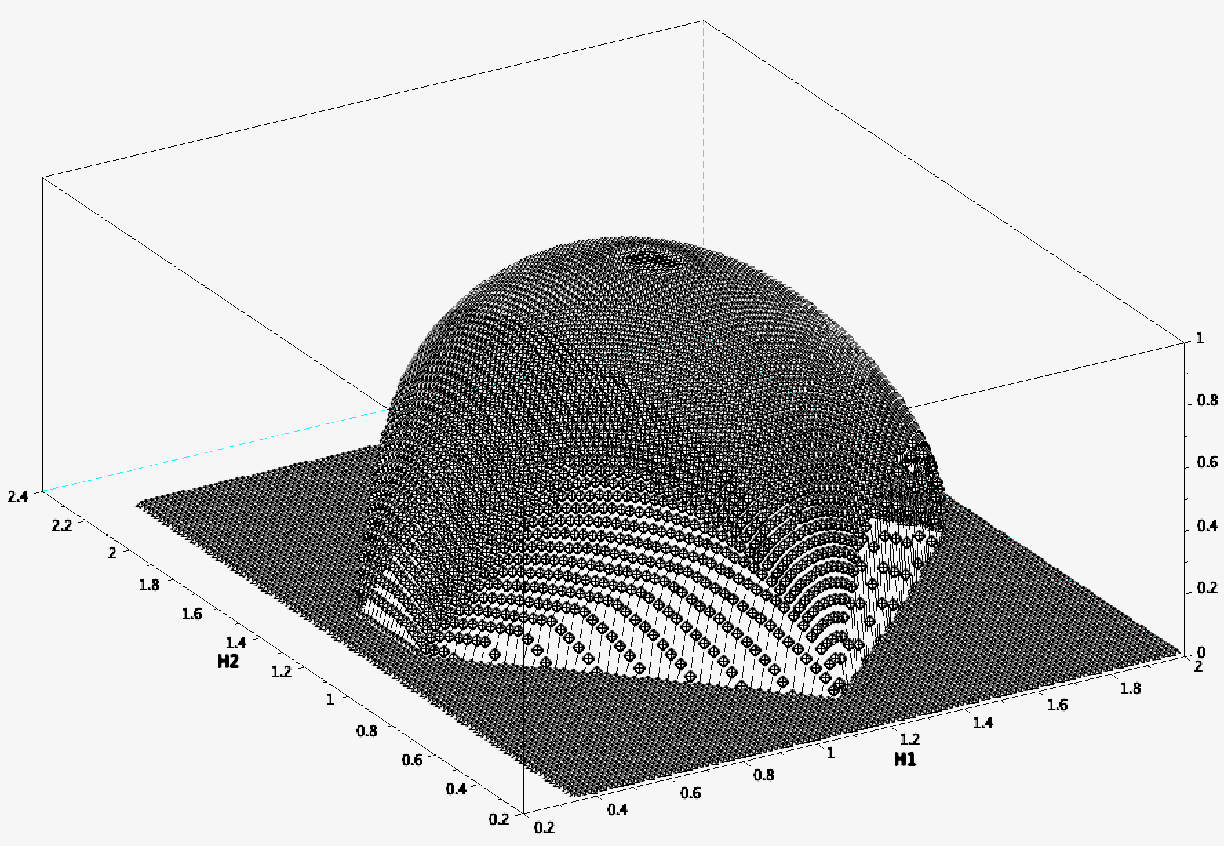
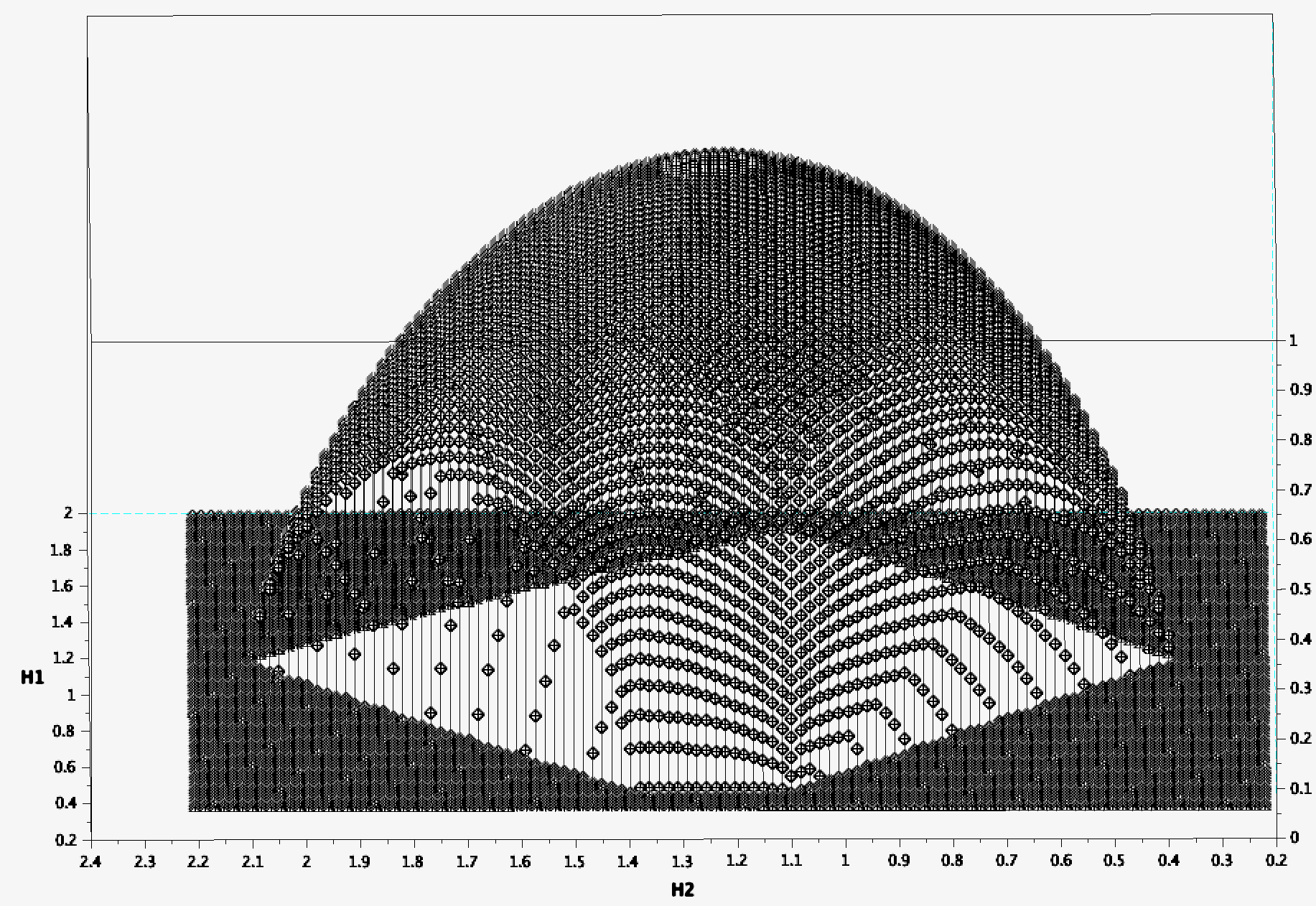
Figure 4. Two views of the Legendre spectrum when $0<p_{1}=0.2<1/2<p_{2}=0.8$ with $\eta=0.5$.

For the second sum, one applies (51) to get for some ${\varepsilon}^{\prime\prime}_{j}$ tending to zero that

$$\Sigma_{2}(j) \sim\sum_{\ell=\lfloor{\varepsilon}^{-2}\rfloor+2}^{j-\lfloor j^{\varepsilon}\rfloor}2^{-\ell T^{\eta}(q_{1},q_{2})}(1-p_{1})^{q_{1}(j-\ell)}p_{1}^{q_{2}\eta(j-\ell)}p_{2}^{q_{2}(1-\eta)(j-\ell)}2^{O(\sqrt{\ell\log\ell}+(j-\ell)^{1/2+{\varepsilon}})}$$

$$\sim\sum_{\ell=\lfloor{\varepsilon}^{-2}\rfloor+2}^{j-\lfloor j^{\varepsilon}\rfloor}2^{-\ell T^{\eta}(q_{1},q_{2})-(j-\ell)\widetilde{T}^{\eta}(q_{1},q_{2})+j{\varepsilon}^{\prime\prime}_{j}}\sim 2^{-j\min(T^{\eta}(q_{1},q_{2}),\widetilde{T}^{\eta}(q_{1},q_{2}))+j{\varepsilon}^{\prime\prime}_{j}}.$$

Finally, for the third term, we observe that $|j-1-\ell|\leq j^{\varepsilon}$, and deduce that for some other sequence ${\varepsilon}^{\prime\prime\prime}_{j}$ tending to zero (we also replace $(j-1)-(j-1)^{\varepsilon}$ by $j-j^{\varepsilon}$ which simplifies the calculation)

$$\Sigma_{3}(j) \sim\sum_{\ell=j-\lfloor j^{\varepsilon}\rfloor}^{j}2^{-\ell T^{\eta}(q_{1},q_{2})}(1-p_{1})^{q_{1}(j-\ell)}p_{1}^{q_{2}\eta(j-\ell)}p_{2}^{q_{2}(1-\eta)(j-\ell)}2^{O(\sqrt{\ell\log\ell}+(j-\ell)^{1/2+{\varepsilon}})}$$

$$\sim 2^{-jT^{\eta}(q_{1},q_{2})+j{\varepsilon}^{\prime\prime\prime}_{j}}.$$

Combining the three previous estimates, one concludes that

$$S(j,q_{1},q_{2}) \sim 2^{-j\min(T^{\eta}(q_{1},q_{2}),\widetilde{T}^{\eta}(q_{1},q_{2}))+j\tilde{\varepsilon}_{j}},$$

where $\tilde{\varepsilon}_{j}\to 0$.

Finally,

$$\sum_{w\in\Sigma_{j}}{\mu_{p_{1}}}(3I_{w})^{q_{1}}\nu_{\eta}(3I_{w})^{q_{2}} \sim 2^{-j\min(T^{\eta}(q_{1},q_{2}),\widetilde{T}^{\eta}(q_{1},q_{2}))+j\tilde{\varepsilon}_{j}}.$$

The result follows. Observe that a phase transition occurs at the curve $\{(q_{1},q_{2}):T^{\eta}(q_{1},q_{2})=\widetilde{T}^{\eta}(q_{1},q_{2})\}$. ∎

The support of $(\widetilde{T}^{\eta})^{*}$ is the parallelogram with same corners as in Section 5, however there is a difference between these two figures, due to the relative positions of $p_{1}$ and $p_{2}$ and the fact that $\delta_{1,2}<0$. Indeed, the four straight lines generating the parallelogram have slopes 1 and $\delta_{1,2}$, which is positive or negative according to whether $p_{1},p_{2}$ are one the same side of $1/2$ or not, respectively, see Figure 4.

Next, observe that $\frac{\partial}{\partial q_{1}}\widetilde{T}^{\eta}(q_{1},q_{2})=\log_{2}(1-p_{1})=H_{1,\min}$ and $\frac{\partial}{\partial q_{2}}\widetilde{T}^{\eta}(q_{1},q_{2})=-\eta\log_{2}(p_{1})-(1-\eta)\log_{2}(p_{2})=\eta H_{1,\max}+(1-\eta)H_{2,\min}$, so these partial derivatives are independent of $q_{1}$ and $q_{2}$. Also, the point $(H_{1,\min},\eta H_{1,\max}+(1-\eta)H_{2,\min})$ lies outside the support of $(T^{\eta})^{*}$. From the elementary properties of the Legendre transform we deduce that:

• $\tau_{{\mu_{p_{1}}},\nu_{\eta}}^{*}$ has support the convex pentagon $\mathcal{P}^{\eta}_{1}$ whose 5 corners are $(H_{1,\min},\eta H_{1,\max}+(1-\eta)H_{2,\min})$ and the four points of the parallelogram described above, see Figure 4.

• $\tau_{{\mu_{p_{1}}},\nu_{\eta}}^{*}$ is the concave hull of the union of the singleton $(H_{1,\min},\eta H_{1,\max}+(1-\eta)H_{2,\min},0)$ and the graph of $(T^{\eta})^{*}$. In particular, it contains a cone constituted by segments all starting from $(H_{1,\min},\eta H_{1,\max}+(1-\eta)H_{2,\min})$ and tangent to the graph of $(T^{\eta})^{*}$, see Figures 2 and 4.

6.2. Computation of the bivariate multifractal spectrum

Let us write $[H_{\eta,\min}:=\eta H_{1,\min}+(1-\eta)H_{2,\min},H_{\eta,\max}:=\eta H_{1,\max}+(1-\eta)H_{2,\max}]$ for the support of $D_{\nu_{\eta}}$.

Assume that for some $x$, $\underline{\dim}({\mu_{p_{1}}},x)=H_{1}$ and $\underline{\dim}(\nu_{\eta},x)=H_{2}$. There exists a sequence $({\varepsilon}_{j})$ depending on $x$ and tending to 0 such that :

• for every $j$ and $\widetilde{I}\in\{I,I^{+},I^{-}\}$, ${\mu_{p_{1}}}(\widetilde{I}_{j}(x))=2^{-jH^{\prime}_{1}}$ where $H^{\prime}_{1}\in[H_{1}-{\varepsilon}_{j},H_{1,\max}+{\varepsilon}_{j}]$ and $\nu_{\eta}(\widetilde{I}_{j}(x))=2^{-jH^{\prime}_{2}}$ where $H^{\prime}_{2}\in[H_{2}-{\varepsilon}_{j},H_{\eta,\max}+{\varepsilon}_{j}]$ (here $H^{\prime}_{1}$ and $H^{\prime}_{2}$ depend on $j$ and $x$),

• there are infinitely many integers $j$ such that ${\mu_{p_{1}}}(\widetilde{I}_{j}(x))\geq 2^{-j(H_{1}+{\varepsilon}_{j})}$ for some $\widetilde{I}\in\{I,I^{+},I^{-}\}$ and, possibly for other integers $j$, $\nu_{\eta}(\widetilde{I}_{j}(x))\geq 2^{-j(H_{2}+{\varepsilon}_{j})}$ for some $\widetilde{I}\in\{I,I^{+},I^{-}\}$.

The same argument as in Lemma 5.5 gives, writing $H^{\prime}_{1}=\eta\alpha+(1-\eta)\beta$ and $H^{\prime}_{2}=\eta\alpha+(1-\eta)G_{1,2}(\beta)$ and letting $j$ tend to infinity, that one necessarily has $(\eta\alpha+(1-\eta)\beta,\eta\alpha+(1-\eta)G(\beta))\in[H_{1},H_{1,\max}]\times[H_{2},H_{\eta,\max}]$, and the two following systems

$$(S_{1})\ \ \begin{cases}H_{1}=\eta\alpha+(1-\eta)\beta\\ H_{2}\leq\eta\alpha+(1-\eta)G_{1,2}(\beta)\end{cases}\ \mbox{ and }\ \ (S_{2})\ \ \begin{cases}H_{1}\leq\eta\alpha+(1-\eta)\beta\\ H_{2}=\eta\alpha+(1-\eta)G_{1,2}(\beta)\end{cases}$$

are realized for infinitely many integers $j$ (not necessarily simultaneously).

Let us first clarify the possible range for the pair of exponents $(H_{1},H_{2})$,

Lemma 6.1.

Almost surely, the support of $D_{{\mu_{p_{1}}},\nu_{\eta}}$ is a (deterministic) pentagon $\mathcal{P}^{\eta}_{2}$ different from $\mathcal{P}^{\eta}_{1}$.

Proof.

Recall that when $0<p_{1}<1/2<p_{2}<1$, $\delta_{1,2}<0$.

$\bullet$ Consider first the system $(S_{1})$. We write $\beta_{H_{1},\alpha}=\frac{H_{1}-\eta\alpha}{1-\eta}$, so that $H_{1}=\eta\alpha+(1-\eta)\beta_{H_{1},\alpha}$.

The exponent $H_{1}$ being fixed, we look for the possible values of $H_{2}$. One can always take $H_{2}=H_{\eta,\min}$, which is the smallest possible value, so we only have to investigate the largest possible value for $H_{2}$.

One rewrites the second line of $(S_{1})$ as $H_{2}\leq H_{1}+(1-\eta)(G_{1,2}(\beta_{H_{1},\alpha})-\beta_{H_{1},\alpha})$. Hence, the largest $\alpha$, the smallest $\beta_{H_{1},\alpha}$ (since $\delta_{1,2}<0$), and the largest $H_{2}$ in $(S_{1})$.

Observe also that by construction $\alpha$ and $\beta$ belong to $[H_{1,\min},H_{1,\max}]$, so

(52) $$\max\big{(}H_{1,\min},\frac{H_{1}-(1-\eta)H_{1,\max}}{\eta}\big{)}\leq\alpha\leq\min\big{(}H_{1,\max},\frac{H_{1}-(1-\eta)H_{1,\min}}{\eta}\big{)}.$$

The two expressions in the above minimum coincide when $H_{1}=(1-\eta)H_{1,\min}+\eta H_{1,\max}$.

1. $H_{1,\min}\leq H_{1}\leq(1-\eta)H_{1,\min}+\eta H_{1,\max}$: the largest possible value for $\alpha$ is $\frac{H_{1}-(1-\eta)H_{1,\min}}{\eta}$. The largest possible $H_{2}$ satisfying $(S_{1})$ is thus $f_{1}(H_{1}):=\eta\frac{H_{1}-(1-\eta)H_{1,\min}}{\eta}+(1-\eta)G_{1,2}(\beta_{H_{1},\frac{H_{1}-(1-\eta)H_{1,\min}}{\eta}})$, and it is checked that $f_{1}$ is the straight line with slope 1 passing through the points $(H_{1,\min},\eta H_{1,\min}+(1-\eta)H_{2,\max})$ and $(\eta H_{1,\max}+(1-\eta)H_{1,\min},H_{\eta,\max})$.

2. $(1-\eta)H_{1,\min}+\eta H_{1,\max}<H_{1}\leq H_{1,\max}$: the largest possible value for $\alpha$ is now constant and equal to $H_{1,\max}$, the corresponding $\beta$ is $\beta_{H_{1},H_{1,\max}}$, and the maximal $H_{2}$ is $\eta H_{1,\max}+(1-\eta)G_{1,2}(\beta_{H_{1},H_{1,\max}}):=f_{2}(H_{1})$. This yields the straight line with slope $\delta_{1,2}$ passing through $(\eta H_{1,\max}+(1-\eta)H_{1,\min},H_{\eta,\max})$ and $(H_{1,\max},\eta H_{1,\max}+(1-\eta)H_{1,\min},)$.

Hence, the possible $(H_{1},H_{2})$ form a pentagon. see Figure 5, top left.

$\bullet$ Next, consider $(S_{2})$. The discussion is quite similar to the one for $(S_{1})$. Indeed, it is always possible to take $H_{1}=H_{1,\min}$ in $(S_{2})$, so $H_{2}$ being fixed, we look for the maximal value for $H_{1}$. Call $\widetilde{\beta}_{H_{2},\alpha}$ the unique solution to $H_{2}=\eta\alpha+(1-\eta)G_{1,2}(\widetilde{\beta}_{H_{2},\alpha})$.

By construction $\alpha$ and $\beta$ belong to $[H_{1,\min},H_{1,\max}]$, so

(53) $$\max\big{(}H_{\eta,\min},\frac{H_{2}-\eta H_{1,\max}}{1-\eta}\big{)}\leq G_{1,2}(\widetilde{\beta}_{H_{2},\alpha})=\frac{H_{2}-\eta\alpha}{1-\eta}\leq\min\big{(}H_{\eta,\max},\frac{H_{2}-\eta H_{1,\min}}{1-\eta}\big{)}.$$

This time we write $H_{1}=H_{2}+(1-\eta)(\beta-G_{1,2}(\beta))$. To get the largest $H_{1}$ one must find the largest $\beta$ satisfying $(S_{2})$. This amounts to taking the minimum in (53). Remark that the two expressions in the above maximum coincide when $H_{2}=H^{\eta}_{2}:=\eta(1-\eta)H_{1,\min}+(\eta+(1-\eta)^{2})H_{1,\max}$. Observe that $\eta(1-\eta)+(\eta+(1-\eta)^{2})=1$, so $H_{1,\min}\leq H_{2}\leq H_{1,\max}$.

1. $H_{\eta,\min}\leq H_{2}\leq H^{\eta}_{2}$: the largest possible value for $G_{1,2}(\beta)$ is constant equal to $H_{\eta,\min}$, the corresponding $H_{1}$ is $\widetilde{f}_{3}(H_{2}):=H_{2}+(1-\eta)(\widetilde{\beta}_{H_{2},\alpha}+G_{1,2}(\widetilde{\beta}_{H_{2},\alpha}))$. Writing the reciprocal function $H_{2}=f_{3}(H_{1})$ of $\widetilde{f}_{3}$, a calculation shows that $f_{3}$ is the straight line with slope 1 passing through the points $(\eta H_{1,\min}+(1-\eta)H_{1,\max},H_{\eta,\min})$ and $(H_{1,\max},\eta H_{1,\max}+(1-\eta)H_{1,\min})$.

2. $H^{\eta}_{2}<H_{2}\leq H_{\eta,\max}$: the largest possible value for $G_{1,2}(\beta)$ is now $\frac{H_{2}-\eta H_{1,\max}}{1-\eta}$, and the maximal $H_{1}$ is $\widetilde{f}_{4}(H_{2}):=H_{2}+(1-\eta)(\widetilde{\beta}_{H_{2},\alpha}+G_{1,2}(\widetilde{\beta}_{H_{2},\alpha}))$. One can check that the reciprocal function $H_{2}=f_{4}(H_{1})$ of $\widetilde{f}_{4}$ coincides with the straight line $f_{2}$ of item (2) obtained above when studying the system $(S_{1})$.

Hence, once again the possible range of $(H_{1},H_{2})$ forms a pentagon, which differs from the one following from $(S_{1})$, see Figure 5, top right.

The intersection $\mathcal{P}^{\eta}_{2}$ between the two above pentagons happens to remain a pentagon with five edges $(H_{1,\min},H_{\eta,\min})$, $(H_{1,\min},\eta H_{1,\min}+(1-\eta)H_{2,\max})$, $(\eta H_{1,\max}+(1-\eta)H_{1,\min},H_{\eta,\max})$, $(H_{1,\max},\eta H_{1,\max}+(1-\eta)H_{1,\min},)$ and $(\eta H_{1,\min}+(1-\eta)H_{1,\max},H_{\eta,\min})$. See again Figure 5, bottom right, for an illustration. ∎

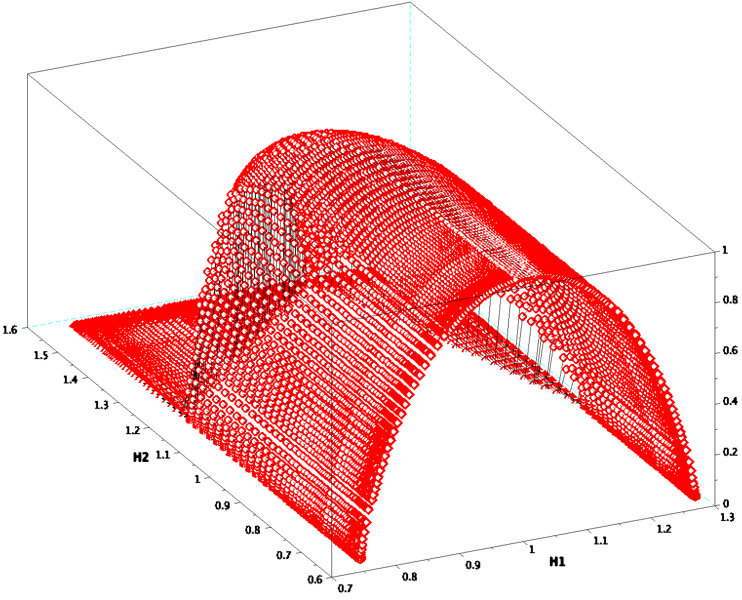
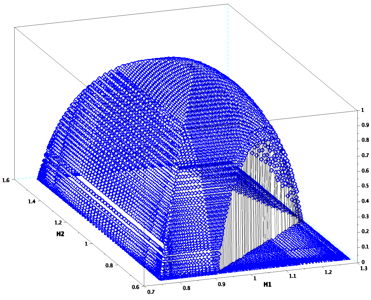
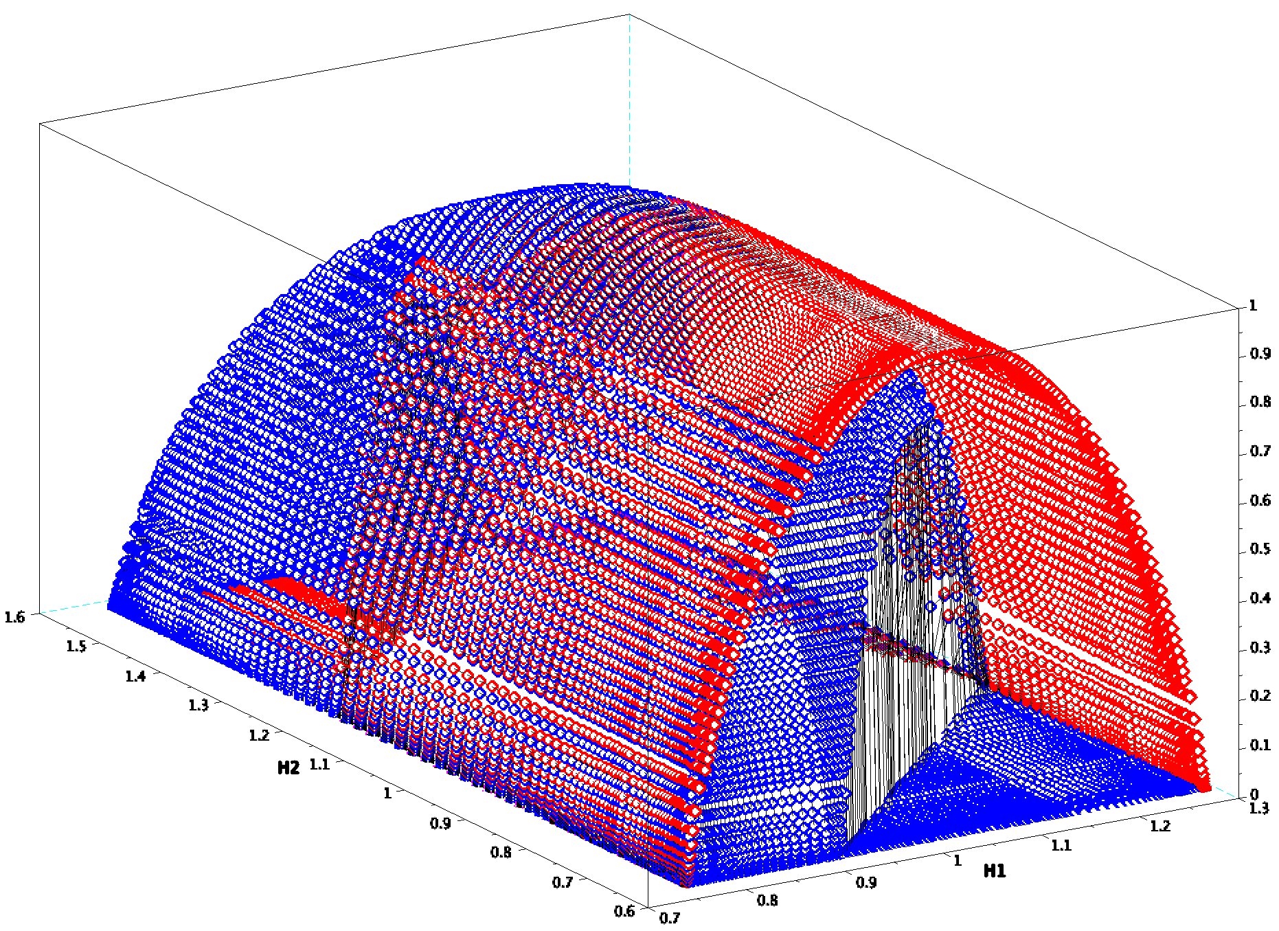
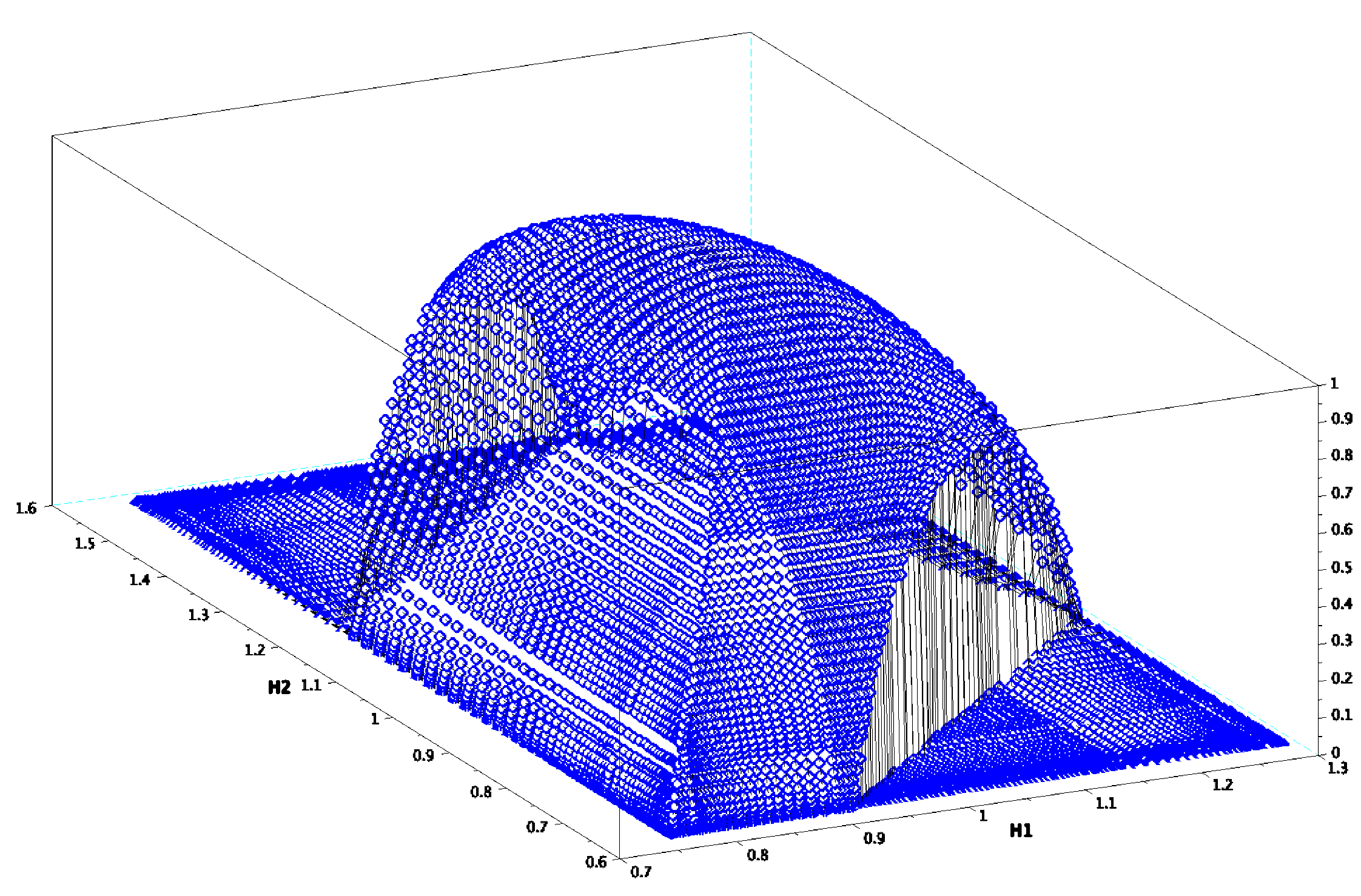
Figure 5. Top: Plot of $D_{1}$ and $D_{2}$ (equations (55) and (56)) when $\eta=0.7$, $p_{1}=0.4$ et $p_{2}=0.8$. Bottom: Superposition of $D_{1}$ and $D_{2}$, and bivariate multifractal spectrum of $({\mu_{p_{1}}},\nu_{\eta})$ (i.e. minimum of $D_{1}$ and $D_{2}$).

We move now to the bivariate multifractal spectrum $D_{{\mu_{p_{1}}},\nu_{\eta}}$. Even if this estimate is not sharp, it is obvious that $D_{{\mu_{p_{1}}},\nu_{\eta}}(H_{1},H_{2})\leq\min(D_{{\mu_{p_{1}}}}(H_{1}),D_{\nu_{\eta}}(H_{2}))$. The term $D_{{\mu_{p_{1}}}}(H_{1})$ is explicit, let us estimate the second one.

Proposition 6.2.

Almost surely, for every $H\in[\eta H_{1,\min}+(1-\eta)H_{2,\min},\eta H_{1,\max}+(1-\eta)H_{2,\max}]$, $D_{\nu_{\eta}}(H)=D_{p_{1},p_{2}}(H)$, where

$$D_{p_{1},p_{2}}(H)=\eta D_{{\mu_{p_{1}}}}(\tau_{\mu_{p_{1}}}^{\prime}(q_{H}))+(1-\eta)D_{{\mu_{p_{2}}}}(\tau_{\mu_{p_{2}}}^{\prime}(q_{H})),$$

and $q_{H}$ is the unique real number such that $H=\eta\tau_{\mu_{p_{1}}}^{\prime}(q_{H})+(1-\eta)\tau_{\mu_{p_{2}}}^{\prime}(q_{H})$.

Proof.

First, the existence and unicity of $q_{H}$ follow from the monotonicity of $\tau_{\mu_{p_{1}}}^{\prime}$ and $\tau_{\mu_{p_{2}}}^{\prime}$.

If for a real number $x$ one has $\underline{\dim}(\nu_{\eta},x)=H_{2}$, then there exists a sequence $({\varepsilon}_{j})$ depending on $x$ and tending to 0 such that :

• for every $j$ and $\widetilde{I}\in\{I,I^{+},I^{-}\}$, $\nu_{\eta}(\widetilde{I}_{j}(x))=2^{-jH^{\prime}}$ where $H^{\prime}\in[H_{2}-{\varepsilon}_{j},\eta H_{1,\max}+(1-\eta)H_{2,\max}+{\varepsilon}_{j}]$,

• there are infinitely many integers $j$ such that $\nu_{\eta}(\widetilde{I}_{j}(x))\geq 2^{-j(H_{2}+{\varepsilon}_{j})}$ for some $\widetilde{I}\in\{I,I^{+},I^{-}\}$.

Consider the interval $\widetilde{I}\in\{I,I^{+},I^{-}\}$ such that $\nu_{\eta}(\widetilde{I}_{j}(x))$ is maximal, and write $\frac{\log{\mu_{p_{1}}}(\widetilde{I}_{j}(x)^{\mathcal{A}})}{2^{-\eta j}}=\eta\alpha_{j}$ and $\frac{\log{\mu_{p_{2}}}(\widetilde{I}_{j}(x)^{\mathcal{A}^{c}})}{2^{-j(1-\eta)}}=\beta_{j}$, so that $\nu_{\eta}(\widetilde{I}_{j}(x))=2^{-j(\eta\alpha_{j}+(1-\eta)\beta_{j})}$. Similar arguments as those used in Lemmas 5.6 and 6.1 imply that there is a subsequence of $(\alpha_{j},\beta_{j})_{j\geq 1}$ such that $(\alpha_{j})$ and $(\beta_{j})$ tend respectively to $\alpha$ and $\beta$ with $\eta\alpha+(1-\eta)\beta=H_{2}$, and that the set of such points has a dimension equal to $\eta D_{{\mu_{p_{1}}}}(\alpha)+(1-\eta)D_{{\mu_{p_{1}}}}(\beta)$. In particular, recalling Proposition 4.4,

$$\bigcup_{\alpha,\beta:\,\eta\alpha+(1-\eta)\beta=H_{2}}E^{p_{1},\mathcal{A}}_{\alpha,\alpha}\cap E^{p_{2},\mathcal{A}^{c}}_{\beta,\beta}\subset E_{\nu_{\eta}}(H).$$

The same arguments as in Lemmas 5.6 and 6.1 also show that with probability one,

$$\dim\Big{(}\bigcup_{\alpha,\beta:\,\eta\alpha+(1-\eta)\beta=H_{2}}E^{p_{1},\mathcal{A}}_{\alpha,\alpha}\cap E^{p_{2},\mathcal{A}^{c}}_{\beta,\beta}\Big{)}=\max_{\alpha,\beta:\,\eta\alpha+(1-\eta)\beta=H_{2}}\big{(}\eta D_{{\mu_{p_{1}}}}(\alpha)+(1-\eta)D_{{\mu_{p_{2}}}}(\beta\big{)},$$

and this last maximum is also an upper bound for the dimension of $E_{\nu_{\eta}}(H)$.

The derivative of $\alpha\mapsto L(\alpha):=\eta D_{{\mu_{p_{1}}}}(\alpha)+(1-\eta)D_{{\mu_{p_{2}}}}(\frac{H_{2}-\eta\alpha}{1-\eta})$ equals $\eta(D^{\prime}_{{\mu_{p_{1}}}}(\alpha)-D^{\prime}_{{\mu_{p_{2}}}}(\frac{H_{2}-\eta\alpha}{1-\eta}))$, which vanishes when $D^{\prime}_{{\mu_{p_{1}}}}(\alpha)=D^{\prime}_{{\mu_{p_{2}}}}(\frac{H_{2}-\eta\alpha}{1-\eta})=D^{\prime}_{{\mu_{p_{2}}}}(\beta)$. Recalling that if $\alpha=\tau_{\mu_{p_{1}}}^{\prime}(q_{\alpha})$, then $D^{\prime}_{{\mu_{p_{1}}}}(\alpha)=q_{\alpha}$ (and similarly for $\beta=\tau_{\mu_{p_{2}}}^{\prime}(q_{\beta})$), one concludes the maximum of $L$ is reached when $q_{\alpha}=q_{\beta}$, hence the result. ∎

Let us estimate the value of $D_{{\mu_{p_{1}}},\nu_{\eta}}$ at every pair $(H_{1},H_{2})\in\mathcal{P}^{\eta}_{2}$. It appears that the upper bound $D_{{\mu_{p_{1}}},\nu_{\eta}}(H_{1},H_{2})\leq\min(D_{{\mu_{p_{1}}}}(H_{1}),D_{\nu_{\eta}}(H_{2}))$ is sharp only on a subset of $\mathcal{P}^{\eta}_{2}$, the exact value of $D_{{\mu_{p_{1}}},\nu_{\eta}}(H_{1},H_{2})$ can be strictly smaller.

Recall the notations $\beta_{H_{1},\alpha}$ and $\widetilde{\beta}_{H_{2},\alpha}$ of the proof of Lemma 6.1, and the systems $(S_{1})$ and $(S_{2})$ of the beginning of Section 6.2.

Definition 6.3.

Define

(54) $$F_{\eta}(\alpha,\beta):=\eta D_{{\mu_{p_{1}}}}(\alpha)+(1-\eta)D_{{\mu_{p_{1}}}}(\beta).$$

For $(H_{1},H_{2})\in[H_{1,\min},H_{1,\max}]\times[H_{\eta,\min},H_{\eta,\max}]$, let us denote

(55) $$D_{1}(H_{1},H_{2}) =\max\{F_{\eta}(\alpha,\beta):(\alpha,\beta)\mbox{ satisfies }(S_{1})\}$$

$$=\max\{F_{\eta}(\alpha,\beta_{H_{1},\alpha}):(\alpha,\beta_{H_{1},\alpha})\mbox{ satisfies }(S_{1})\}$$

(56) $$D_{2}(H_{1},H_{2}) =\max\{F_{\eta}(\alpha,\beta):(\alpha,\beta)\mbox{ satisfies }(S_{2})\}$$

$$=\max\{F_{\eta}(\alpha,\widetilde{\beta}_{H_{2},\alpha}):(\alpha,\widetilde{\beta}_{H_{2},\alpha})\mbox{ satisfies }(S_{2})\}.$$

Observe that in (55) and (56), once $H_{1}$, $H_{2}$ and $\alpha$ are fixed, the parameter $\beta$ is actually entirely determined by $\alpha$ (this is what is expressed in the second equation defining $D_{1}$ and $D_{2}$), so $\alpha$ is actually the only moving parameter in the maxima to be computed.

Proposition 6.4.

Almost surely, for every $(H_{1},H_{2})\in\mathcal{P}^{\eta}_{2}$,

$$D_{{\mu_{p_{1}}},\nu_{\eta}}(H_{1},H_{2})=\min(D_{1}(H_{1},H_{2}),D_{2}(H_{1},H_{2})).$$

Proof.

Fix $(H_{1},H_{2})\in\mathcal{P}^{\eta}_{2}$. When $\underline{\dim}({\mu_{p_{1}}},x)=H_{1}$ and $\underline{\dim}(\nu_{\eta},x)=H_{2}$, items (i) and (ii) of the beginning of Section 6.2 hold.

Let us call $\mathcal{G}(H_{1},H_{2},\alpha,\beta)$ the sets of points $y\in[0,1]$ such that $(S_{1})$ is satisfied by the quadruplet $(H_{1},H_{2},\alpha,\beta)$, $\underline{\dim}({\mu_{p_{1}}},y)=H_{1}$ and $\underline{\dim}(\nu_{\eta},y)\geq H_{2}$.

Similarly, call $\widetilde{\mathcal{G}}(H_{1},H_{2},\alpha,\beta)$ the sets of points $y\in[0,1]$ such that $(S_{2})$ is satisfied by the quadruplet $(H_{1},H_{2},\alpha,\beta)$, $\underline{\dim}({\mu_{p_{1}}},y)\geq H_{1}$ and $\underline{\dim}(\nu_{\eta},y)=H_{2}$.

By construction, when $\underline{\dim}({\mu_{p_{1}}},x)=H_{1}$ and $\underline{\dim}(\nu_{\eta},x)=H_{2}$, $x$ must belong to

$$\Big{(}\bigcup_{\alpha,\beta\in[H_{1,\min},H_{1,\max}]}\mathcal{G}(H_{1},H_{2},\alpha,\beta)\Big{)}\cap\Big{(}\bigcup_{\alpha,\beta\in[H_{1,\min},H_{1,\max}]}\widetilde{\mathcal{G}}(H_{1},H_{2},\alpha,\beta)\Big{)}.$$

Lemma 6.5.

There exist a unique value $\alpha_{H_{1},H_{2}}$ such that $D_{1}(H_{1},H_{2})=F_{\eta}(\alpha_{H_{1},H_{2}},\beta_{H_{1},\alpha_{H_{1},H_{2}}})$, and a unique value $\widetilde{\alpha}_{H_{1},H_{2}}$ such that $D_{2}(H_{1},H_{2})=F_{\eta}(\widetilde{\alpha}_{H_{1},H_{2}},\widetilde{\beta}_{H_{2},\widetilde{\alpha}_{H_{1},H_{2}}})$.

This lemma simply follows from the strict concavity of $D_{{\mu_{p_{1}}}}$ and the fact that the range of possible $\alpha$’s in (55) and (56) is an interval.

A standard discretization argument (identical to the one used in the proof of Lemma 5.6) shows that the Hausdorff dimension of the union of sets $\bigcup_{\alpha,\beta\in[H_{1,\min},H_{1,\max}]}\mathcal{G}(H_{1},H_{2},\alpha,\beta)$ is reached for the pair $(\alpha_{H_{1},H_{2}},\beta_{H_{1},\alpha_{H_{1},H_{2}}})$, and similarly for the sets $\widetilde{\mathcal{G}}(H_{1},H_{2},\alpha,\beta)$ with the exponents $(\widetilde{\alpha}_{H_{1},H_{2}},\widetilde{\beta}_{H_{2},\widetilde{\alpha}_{H_{1},H_{2}}})$.

In particular,

(57) $$D_{{\mu_{p_{1}}},\nu_{\eta}}(H_{1},H_{2})\leq\min\Big{(}F_{\eta}\big{(}\alpha_{H_{1},H_{2}},\beta_{H_{1},\alpha_{H_{1}H_{2}}}\big{)},F_{\eta}\big{(}\widetilde{\alpha}_{H_{1},H_{2}},\widetilde{\beta}_{H_{2},\widetilde{\alpha}_{H_{1},H_{2}}}\big{)}\Big{)}.$$

The conclusion follows from the next proposition, that we prove just hereafter.

Proposition 6.6.

Let $(H_{1},H_{2})\in\mathcal{P}^{\eta}_{2}$, and let $(\alpha,\alpha^{\prime},\beta,\beta^{\prime})$ be such that $(\alpha,\beta)$ and $(\alpha^{\prime},\beta^{\prime})$ satisfy respectively the systems $(S_{1})$ and $(S_{2})$. Then

$$\dim{\mathcal{G}}(H_{1},H_{2},\alpha,\beta)\cap\widetilde{\mathcal{G}}(H_{1},H_{2},\alpha^{\prime},\beta^{\prime})=\min(F_{\eta}(\alpha,\beta),F_{\eta}(\alpha^{\prime},\beta^{\prime})).$$

From Proposition 6.6 we deduce that the dimension of $\mathcal{G}(H_{1},H_{2},\alpha_{H_{1},H_{2}},\beta_{H_{1},\alpha_{H_{1}H_{2}}})\cap\widetilde{\mathcal{G}}(H_{1},H_{2},\widetilde{\alpha}_{H_{1},H_{2}},\widetilde{\beta}_{H_{1},\widetilde{\alpha}_{H_{1}H_{2}}})$ equals the right-hand-side of (57) above, hence concluding to the equality in the last equation. ∎

We now conclude by proving Proposition 6.6.

Proof of Proposition 6.6.

Recall that in the situation of Proposition 6.6, $\beta=\beta_{H_{1},\alpha}=\frac{H_{1}-\eta\alpha}{1-\eta}$ and $\beta^{\prime}=\widetilde{\beta}_{H_{2}.\alpha^{\prime}}$ (the unique solution to $H_{2}=\eta\alpha+(1-\eta)G_{1,2}(\widetilde{\beta}_{H_{2},\alpha})$).

Call $\delta=\min(F_{\eta}(\alpha,\beta),F_{\eta}(\alpha^{\prime},\beta^{\prime}))$. We build a measure $\nu$ of dimension $\delta$ that is supported by ${\mathcal{G}}(H_{1},H_{2},\alpha,\beta)\cap\widetilde{\mathcal{G}}(H_{1},H_{2},\alpha^{\prime},\beta^{\prime})$.

Lemma 4.2 is applied to the four parameters $\widetilde{p}_{\gamma}$ for $\gamma\in\{\alpha,\beta,\alpha^{\prime},{\beta^{\prime}}\}$. Recall that $\widetilde{p}_{\gamma}$ is the unique real number such that $H_{\widetilde{p}_{\gamma},e}=D_{\mu_{\widetilde{p}_{\gamma}}}(H_{\widetilde{p}_{\gamma},e})=\tau_{{\mu_{p_{1}}}}^{*}(\gamma)=D_{{\mu_{p_{1}}}}(\gamma)$.

Fix ${\varepsilon}<1/100$, and consider the sequence $(\widetilde{J}_{n})_{n\geq 1}$ defined by

$$\widetilde{J}_{n}=\max(\max(J_{p_{1},p_{2},\gamma,n,{\varepsilon}}:\gamma\in\{\alpha,\beta,\alpha^{\prime},{\beta^{\prime}}\}),\widetilde{J}_{n-1}+2),$$

so that the four sets $\mathcal{E}_{p_{1},p_{2},\gamma,n,{\varepsilon}}$ satisfy that $\mu_{\widetilde{p}_{\gamma}}(\mathcal{E}_{p_{1},p_{2},\gamma,n,{\varepsilon}})\geq 1-{\varepsilon}2^{-n-2}$ for the same sequence $\widetilde{J}_{n}$ (instead of $J_{p_{1},p_{2},\gamma,n,{\varepsilon}}$) in (36).

Call $\gamma_{1}=\min(H_{1,\max},H_{2,\max})/2$, $\gamma_{2}=2\times\max(H_{1,\max},H_{2,\max})$, and consider an increasing sequence $(J_{n})_{n\geq 0}$ of integers with $J_{0}=\widetilde{J}_{1}$ and such that for every $n\geq 1$:

• ${J_{n}}2^{-n}\geq(J_{n}+2)^{{\varepsilon}_{J_{n}}}$ and $\sqrt{2^{-n}(J_{n}+2)\log(2^{-n}(J_{n}+2))/{\varepsilon}_{\widetilde{J}_{n+1}}}\leq 2^{-n-3}J_{n}$.

• $J_{n}\geq\widetilde{J}_{n-1}+\widetilde{J}_{n}+1$,

• $2^{-n-3}(J_{n}-J_{n-1})\geq\frac{\gamma_{2}}{\gamma_{1}}\widetilde{J}_{n}$.

• $J_{n}\geq\max(\frac{2J_{n-1}}{\gamma_{1}},2^{(n+3)\frac{\gamma_{2}}{\gamma_{1}}})$.

In the first property, ${\varepsilon}^{J}$ refers to Lemma 4.3. This property, combined with (38), implies that for every $j\geq 2^{-n}J_{n}$,

(58) $$|\#\mathcal{A}_{J_{n},J_{n}+j}-\eta j| \leq 2^{-n-2}j\ \ \mbox{ and }\ \ |\#\mathcal{A}^{c}_{J_{n},J_{n}+j}-(1-\eta)j|\leq 2^{-n-2}j.$$

We set $P_{1}=0$, and we assume that the mass of the measure $\nu$ is given on every interval $I\in\Sigma_{P_{2n+1}}$ for some integer $n\geq 0$.

Recall (37), and set for any integer $n$

(59) $${\widetilde{\mathcal{A}}}_{n}=(\mathcal{A}-{n})\cap\mathbb{N}^{*}\ \mbox{ and }\ \ {\widetilde{\mathcal{A}}}^{c}_{n}=(\mathcal{A}^{c}-{n})\cap\mathbb{N}^{*}.$$

$\bullet$ Step $2n+2$: Choose an integer $P_{2n+2}$ so large that $\min(\#\mathcal{A}_{P_{2n+1},P_{2n+2}},\#\mathcal{A}^{c}_{P_{2n+1},P_{2n+2}})\geq J_{2n+2}$ (in particular, $P_{2n+2}-P_{2n+1}\geq J_{2n+2}$). For every $I_{w}\in{\Sigma}_{P_{2n+2}}$, write $w=w_{|P_{2n+1}}w^{\prime}$ for $w^{\prime}\in\Sigma_{P_{2n+2}-P_{2n+1}}$, and set

$$\nu(I_{w})=\nu(I_{w_{|P_{2n+1}}})\mu_{\widetilde{p}_{\alpha}}(I_{w^{\prime}}^{{\widetilde{\mathcal{A}}}_{P_{2n+1}}})\mu_{\widetilde{p}_{\beta}}(I_{w^{\prime}}^{{\widetilde{\mathcal{A}}}_{P_{2n+1}}^{c}}).$$

$\bullet$ Step $2n+3$: As above, choose $P_{2n+3}$ so large that $\min(\#\mathcal{A}_{P_{2n+2},P_{2n+3}},\#\mathcal{A}^{c}_{P_{2n+2},P_{2n+3}})\geq J_{2n+3}$. For every $I_{w}\in{\Sigma}_{P_{2n+3}}$, write $w=w_{|P_{2n+2}}w^{\prime}$ for $w^{\prime}\in\Sigma_{P_{2n+3}-P_{2n+2}}$, and set

$$\nu(I_{w})=\nu(I_{w_{|P_{2n+2}}})\mu_{\widetilde{p}_{\alpha^{\prime}}}(I_{w^{\prime}}^{{\widetilde{\mathcal{A}}}_{P_{2n+2}}})\mu_{\widetilde{p}_{{\beta^{\prime}}}}(I_{w^{\prime}}^{{\widetilde{\mathcal{A}}}_{P_{2n+2}}^{c}}).$$

The intuition is that at generation $P_{2n+2}$, for the intervals carrying the mass of the measure $\nu$, ${\mu_{p_{1}}}(I)\sim|I|^{\eta\alpha+(1-\eta)\beta}$ and $\nu_{\eta}(I)\sim|I|^{\eta\alpha+(1-\eta)G_{1,2}(\beta)}$, while at generation $P_{2n+3}$, ${\mu_{p_{1}}}(I)\sim|I|^{\eta\alpha^{\prime}+(1-\eta)\beta^{\prime}}$ and $\nu_{\eta}(I)\sim|I|^{\eta\alpha^{\prime}+(1-\eta)G_{1,2}(\beta^{\prime})}$.

We now list the properties of the measure $\nu$ we constructed, together with those of ${\mu_{p_{1}}}$ and ${\mu_{p_{2}}}$.

Lemma 6.7.

Write the dyadic decomposition of $x\in[0,1]$ as $x=0,x_{1}x_{2}....x_{n}..$, where $x_{n}\in\Sigma_{P_{n+1}-P_{n}}$. Consider

$$\mathcal{I}_{2n,{\varepsilon}}=\left\{I\in\Sigma_{P_{2n+1}-P_{2n}}:\begin{cases}I^{{\widetilde{\mathcal{A}}}_{P_{2n-1}}}\mbox{ contains a point }x\in\mathcal{E}_{p_{1},p_{2},\alpha,n,{\varepsilon}}\\ I^{{\widetilde{\mathcal{A}}}_{P_{2n-1}}^{c}}\mbox{ contains a point }x\in\mathcal{E}_{p_{1},p_{2},\beta,n,{\varepsilon}}\end{cases}\right\}$$

and

$$\mathcal{I}_{2n+1,{\varepsilon}}=\left\{I\in\Sigma_{P_{2n+2}-P_{2n+1}}:\begin{cases}I^{{\widetilde{\mathcal{A}}}_{P_{2n}}}\mbox{ contains a point }x\in\mathcal{E}_{p_{1},p_{2},\alpha^{\prime},n,{\varepsilon}}\\ I^{{\widetilde{\mathcal{A}}}_{P_{2n}}^{c}}\mbox{ contains a point }x\in\mathcal{E}_{p_{1},p_{2},\beta^{\prime},n,{\varepsilon}}\end{cases}\right\}$$

Finally, let

$$E(\nu,{\varepsilon})=\Big{\{}x\in[0,1]:\ \forall\,n\geq 1,\ x_{n}\in\bigcup_{I\in\mathcal{I}_{n,{\varepsilon}}}I\Big{\}}.$$

Then $\nu(E(\nu,{\varepsilon}))\geq 1-{\varepsilon}$.

Proof.

By construction, for every $n$, $\mu_{\widetilde{p}_{\alpha}}(\bigcup_{I\in\mathcal{I}_{n,{\varepsilon}}}I^{{\widetilde{\mathcal{A}}}_{P_{n}}})\geq\mu_{\widetilde{p}_{\alpha}}(\mathcal{E}_{p_{1},p_{2},\alpha,n,{\varepsilon}})\geq 1-{\varepsilon}2^{-n-2}$ and $\mu_{\widetilde{p}_{\beta}}(\bigcup_{I\in\mathcal{I}_{n,{\varepsilon}}}I^{{\widetilde{\mathcal{A}}}_{P_{n}}^{c}})\geq\mu_{\widetilde{p}_{\beta}}(\mathcal{E}_{p_{1},p_{2},\beta,n,{\varepsilon}})\geq 1-{\varepsilon}2^{-n-2}$.

Hence, if $x=0,x_{1}x_{2}....x_{n}..$, where $x_{n}\in\Sigma_{P_{n+1}-P_{n}}$, $\nu\Big{(}\Big{\{}x\in[0,1]:\ x_{n}\in\bigcup_{I\in\mathcal{I}_{n,{\varepsilon}}}I\Big{\}}\Big{)}\geq 1-{\varepsilon}2^{-n-1}$. Finally,

$$\nu(E(\nu,{\varepsilon})^{c}) \leq\sum_{n=1}^{\infty}\nu\Big{(}\Big{\{}x\in[0,1]:\ x_{n}\in\bigcup_{I\in\mathcal{I}_{n,{\varepsilon}}}I\Big{\}}\Big{)}\leq 2\sum_{n=1}^{\infty}\ {\varepsilon}2^{-n-1}\leq{\varepsilon}.$$

∎

From the definitions and the assumptions (A1-4) on $J_{n}$, for every $x\in E(\nu,{\varepsilon})$, for every $n\geq 1$:

1. $I^{\mathcal{A}}_{P_{2n+1}}(x)$ satisfies $\mathcal{P}(p_{1},p_{2},\alpha^{\prime},{\varepsilon},P_{2n+1}^{\mathcal{A}})$ and $I^{\mathcal{A}^{c}}_{P_{2n+1}}(x)$ satisfies $\mathcal{P}(p_{1},p_{2},{\beta^{\prime}},{\varepsilon},P_{2n+1}^{\mathcal{A}^{c}})$.

2. $I^{\mathcal{A}}_{P_{2n+2}}(x)$ satisfies $\mathcal{P}(p_{1},p_{2},\alpha,{\varepsilon},P_{2n+2}^{\mathcal{A}})$ and $I^{\mathcal{A}^{c}}_{P_{2n+2}}(x)$ satisfies $\mathcal{P}(p_{1},p_{2},\beta,{\varepsilon},P_{2n+2}^{\mathcal{A}^{c}})$.

Lemma 6.8.

For every $n\geq 1$, every $\alpha$, every $I\in\Sigma_{P_{2n+1}}$, if $I^{\mathcal{A}}$ satisfies $\mathcal{P}(p_{1},p_{2},\alpha^{\prime},n,P_{2n+1}^{\mathcal{A}})$ and $I^{\mathcal{A}^{c}}$ satisfies $\mathcal{P}(p_{1},p_{2},{\beta^{\prime}},n,P_{2n+1}^{\mathcal{A}^{c}})$, then for every $\widetilde{I}\in\{I,I^{+},I^{-}\}$,

$$2^{-{P_{2n+1}}(\eta\alpha^{\prime}+(1-\eta){\beta^{\prime}}+2^{-n})} \leq{\mu_{p_{1}}}(\widetilde{I})\leq 2^{-{P_{2n+1}}(\eta\alpha^{\prime}+(1-\eta){\beta^{\prime}}-2^{-n})}$$

$$2^{-{P_{2n+1}}(\eta\alpha^{\prime}+(1-\eta)G_{1,2}({\beta^{\prime}})+2^{-n})} \leq\nu_{\eta}(\widetilde{I})\leq 2^{-{P_{2n+1}}(\eta\alpha^{\prime}+(1-\eta)G_{1,2}({\beta^{\prime}})-2^{-n})}$$

$$2^{-{P_{2n+1}}(F_{\eta}(\alpha^{\prime},{\beta^{\prime}})+2^{-n})} \leq\nu(\widetilde{I})\leq 2^{-{P_{2n+1}}(F_{\eta}(\alpha^{\prime},{\beta^{\prime}})-2^{-n})}.$$

Proof.

This directly follows from the following arguments:

• $|P_{n}^{\mathcal{A}}-\eta P_{n}|\leq 2^{-n-2}P_{n}$ and $|P_{n}^{\mathcal{A}^{c}}-(1-\eta)P_{n}|\leq 2^{-n-2}P_{n}$ by $(A1)$,

• the previous lemmas,

• the multiplicative formulas ${\mu_{p_{1}}}(I)={\mu_{p_{1}}}(I^{\mathcal{A}}){\mu_{p_{1}}}(I^{\mathcal{A}^{c}})$, $\nu_{\eta}(I)={\mu_{p_{1}}}(I^{\mathcal{A}}){\mu_{p_{2}}}(I^{\mathcal{A}^{c}})$ and $\nu(I)=\mu_{\widetilde{p}_{\alpha}}(I^{\mathcal{A}})\mu_{\widetilde{p}_{\beta}}(I^{\mathcal{A}^{c}})$,

• the assumptions $(A3)$ and $(A4)$ on $P_{n}$,

• if $\widetilde{I}$ is one of the two neighbors of $I$, then $\widetilde{I}^{\mathcal{A}}$ and $\widetilde{I}^{\mathcal{A}^{c}}$ also respectively satisfy (35).

∎

Lemma 6.9.

For every $n\geq 1$, every $\alpha$, every $I\in\Sigma_{P_{2n+2}}$, if $I^{\mathcal{A}}$ satisfies $\mathcal{P}(p_{1},p_{2},\alpha,n,P_{2n+2}^{\mathcal{A}})$ and $I^{\mathcal{A}^{c}}$ satisfies $\mathcal{P}(p_{1},p_{2},\beta,n,P_{2n+2}^{\mathcal{A}^{c}})$, then for every $\widetilde{I}\in\{I,I^{+},I^{-}\}$,

$$2^{-P_{2n+2}(\eta\alpha+(1-\eta)\beta+2^{-n})} \leq{\mu_{p_{1}}}(\widetilde{I})\leq 2^{-P_{2n+2}(\eta\alpha+(1-\eta)\beta-2^{-n})}$$

$$2^{-P_{2n+2}(\eta\alpha+(1-\eta)G_{1,2}(\beta)+2^{-n})} \leq\nu_{\eta}(\widetilde{I})\leq 2^{-P_{2n+2}(\eta\alpha+(1-\eta)G_{1,2}(\beta)-2^{-n})}$$

$$2^{-P_{2n+2}(F_{\eta}(\alpha,\beta)+2^{-n})} \leq\nu(\widetilde{I})\leq 2^{-P_{2n+2}(F_{\eta}(\alpha,\beta_{\alpha})-2^{-n})}.$$

Proof.

It is identical to the previous lemma replacing $P_{2n+1}$ by $P_{2n+2}$, $\alpha^{\prime}$ by $\alpha$ and ${\beta^{\prime}}$ by $\beta$.∎

Lemma 6.10.

With probability one, for every $x\in E(\nu,{\varepsilon})$, $\underline{\dim}({\mu_{p_{1}}},x)=H_{1}$ and $\underline{\dim}(\nu_{\eta},x)=H_{2}$, and $\underline{\dim}(\nu,x)=\min(F_{\eta}(\alpha,\beta),F_{\eta}(\alpha^{\prime},\beta^{\prime}))$.

Proof.

We prove the claim for $\nu_{\eta}$, the proof is similar for ${\mu_{p_{1}}}$ and $\nu$.

By the second equations of Lemma 6.8 and Lemma 6.9, and recalling that

(60) $$H_{2}=\eta\alpha^{\prime}+(1-\eta)G_{1,2}(\beta^{\prime})\leq\eta\alpha+(1-\eta)G_{1,2}(\beta)$$

by the systems $(S_{1})$ and $(S_{2})$, it is enough to show that when $j\in[P_{n}+1,P_{n+1}-1]$, $\nu_{\eta}(\widetilde{I})\leq 2^{-j(H_{2}-K2^{-n})}$ (for some constant $K$ independent of $n$ and $j$).

Let us prove it for $j\in[P_{2n}+1,P_{2n+1}-1]$, the other case $j\in[P_{2n+1}+1,P_{2n+2}-1]$ is identical.

At generation $P_{2n}$, the second equation of Lemma 6.9 holds.

Then, let $I\in\Sigma_{P_{2n}}$ containing some $x\in E(\nu,{\varepsilon})$, and write $x=0,x_{1}x_{2}....x_{n}..$, with $x_{n}\in\Sigma_{P_{n+1}-P_{n}}$. So , using (59), $x_{2n}$ belongs to some interval $L\in\Sigma_{P_{2n+1}-P_{n}}$ such that $L^{\mathcal{A}_{P_{2n}}}\in E_{p_{1},p_{2},\alpha,n,{\varepsilon}}$ and $L^{\mathcal{A}_{P_{2n}}^{c}}\in E_{p_{1},p_{2},\beta,n,{\varepsilon}}$.

Write the dyadic coding of $I_{j}(x)$ as $x_{1}x_{2}...x_{2n}w_{j}(x)$, and call $L_{j}(x)\in\Sigma_{j-P_{2n}}$ the dyadic interval whose dyadic coding is $w_{j}(x)$. One has by construction

$$\nu_{\eta}(I_{j}(x))= \nu_{\eta}(I){\mu_{p_{1}}}(L^{\mathcal{A}_{P_{2n}}}_{j}(x)){\mu_{p_{2}}}(L_{j}^{\mathcal{A}_{P_{2n}}^{c}}(x))$$

where by Lemma 6.9,

$$2^{-j(\eta\alpha+(1-\eta)G_{1,2}(\beta)+2^{-n})} \leq\nu_{\eta}(I)\leq 2^{-j(\eta\alpha+(1-\eta)G_{1,2}(\beta)-2^{-n})}.$$

• Assume that $j\in[P_{2n}+1,P_{2n}(1+2^{-n})]$: one has by construction

  $$\nu_{\eta}(I_{j}(x)) \leq\nu_{\eta}(I)\leq 2^{-P_{2n}(\eta\alpha+(1-\eta)G_{1,2}(\beta)-2^{-n})}=2^{-j\frac{P_{2n}}{j}(\eta\alpha+(1-\eta)G_{1,2}(\beta)-2^{-n})}.$$

  But by (A4), $\frac{P_{2n}}{j}\geq 1-2^{-n}$, so

  $$\nu_{\eta}(I_{j}(x))\leq 2^{-j(\eta\alpha+(1-\eta)G_{1,2}(\beta)-2^{-n})(1-2^{-n})}\leq 2^{-j(\eta\alpha+(1-\eta)G_{1,2}(\beta)-(\gamma_{2}+1)2^{-n})}\leq 2^{-j(H_{2}-(\gamma_{2}+1)2^{-n})}.$$

• Assume that $j\in[P_{2n}(1+2^{-n}),P_{2n+1}-1]$: By definition of $E(\nu,{\varepsilon})$, ${\mu_{p_{1}}}(L_{j}^{\mathcal{A}_{P_{2n}}}(x))\leq 2^{-\#\mathcal{A}_{P_{2n},j}(\alpha^{\prime}-2^{-n-2})}$ and ${\mu_{p_{2}}}(L_{j}^{\mathcal{A}_{P_{2n}}^{c}}(x))\leq 2^{-\#\mathcal{A}_{P_{2n},j}^{c}(G_{1,2}(\beta^{\prime})-2^{-n-2})}$. Hence,

  $$\nu_{\eta}(I_{j}(x)) \leq 2^{-P_{2n}(\eta\alpha+(1-\eta)G_{1,2}(\beta)-2^{-n})}2^{-\#\mathcal{A}_{P_{2n},j}(\alpha^{\prime}-2^{-n-2})}2^{-\#\mathcal{A}_{P_{2n},j}^{c}(G_{1,2}(\beta^{\prime})-2^{-n-2})}.$$

  By definition of $P_{2n}$, $|\#\mathcal{A}_{P_{2n},j}-\eta(j-P_{2n})|\leq 2^{-n-2}(j-P_{2n})$ and $|\#\mathcal{A}^{c}_{P_{2n},j}-(1-\eta)(j-P_{2n})|\leq 2^{-n-2}(j-P_{2n})$, so

  $$\nu_{\eta}(I_{j}(x)) \leq 2^{-P_{2n}(\eta\alpha+(1-\eta)G_{1,2}(\beta))+(j-P_{2n})(\eta\alpha^{\prime}+(1-\eta)G_{1,2}(\beta^{\prime}))}2^{t},$$

  where $t=2^{-n}P_{2n}+2^{-n-2}(j-P_{2n})(\alpha^{\prime}-2^{-n-2})+\eta(j-P_{2n})2^{-n-2}+2^{-n-2}(j-P_{2n})(G_{1,2}(\beta^{\prime})-2^{-n-2}+(1-\eta)(j-P_{2n})2^{-n-2}$. A quick estimate shows that $t\leq(\gamma_{2}+2)2^{-n}j$. Hence, recalling (60), one concludes that

  $$\nu_{\eta}(I_{j}(x)) \leq 2^{-j(H_{2}-(\gamma_{2}+2)2^{{}_{n}})}.$$

One concludes that ${\varepsilon}>0$ being fixed, for every sufficiently large integer $j$, $\nu_{\eta}(I_{j}(x))\leq 2^{-j(H_{2}-{\varepsilon})}$. This yields that $\underline{\dim}(\nu_{\eta},x)\geq H_{2}-{\varepsilon}$. Also, by Lemma 6.8 $\nu_{\eta}(I_{j}(x))\geq 2^{-j(H_{2}+{\varepsilon})}$ for infinitely many integers $j$, so $\underline{\dim}(\nu_{\eta},x)\leq H_{2}+{\varepsilon}$. Letting ${\varepsilon}$ tend to zero gives the result.

∎

Finally, we proved that for all $x\in E(\nu,{\varepsilon})$, $\underline{\dim}(\nu,x)=\delta$. This holds for every ${\varepsilon}$, and since $\nu(E(\nu,{\varepsilon}))\geq 1-{\varepsilon}$, one derives that for $\nu$-almost every $x$, $\underline{\dim}(\nu,x)=\delta$, $\underline{\dim}({\mu_{p_{1}}},x)=H_{1}$ and $\underline{\dim}(\nu_{\eta},x)=H_{2}$. Applying Billingsley’s Lemma allows then to conclude the proof of Proposition 6.6. ∎

6.3. Failure of the bivariate multifractal formalism

Since the multifractal spectrum has a support strictly larger than the support of the Legendre spectrum, it is obvious that the pair $({\mu_{p_{1}}},\nu_{\eta})$ does not satisfy the bivariate multifractal formalism.

Even if we do not elaborate on this, the two spectra do not coincide on the intersection of their support either (see Figure 6). Indeed, it can be checked that $D_{{\mu_{p_{1}}},\nu_{\eta}}$ is strictly concave. Since the Legendre spectrum has a conic shape on one part of its support, the two spectra may coincide only on the other part of the support, i.e. where the Legendre spectrum $\tau_{{\mu_{p_{1}}},\nu_{\eta}}^{*}$ is given by $(T^{\eta})^{*}$.

Recalling (48) which gives an alternative formula for $(T^{\eta})^{*}(H_{1},H_{2})$, one sees that $D_{1}$ and $(T^{\eta})^{*}$ coincide when in Lemma 6.5 $\mathcal{M}(\alpha_{H_{1},H_{2}},\beta_{H_{1},\alpha_{H_{1},H_{2}}})=(H_{1},H_{2})$, and that $D_{2}$ and $(T^{\eta})^{*}$ coincide when $\mathcal{M}(\widetilde{\alpha}_{H_{1},H_{2}},\widetilde{\beta}_{H_{1},\widetilde{\alpha}_{H_{1},H_{2}}})=(H_{1},H_{2})$. This defines two distinct regions in the plane, with non-empty intersection. In particular, the two spectra coincide on the segment

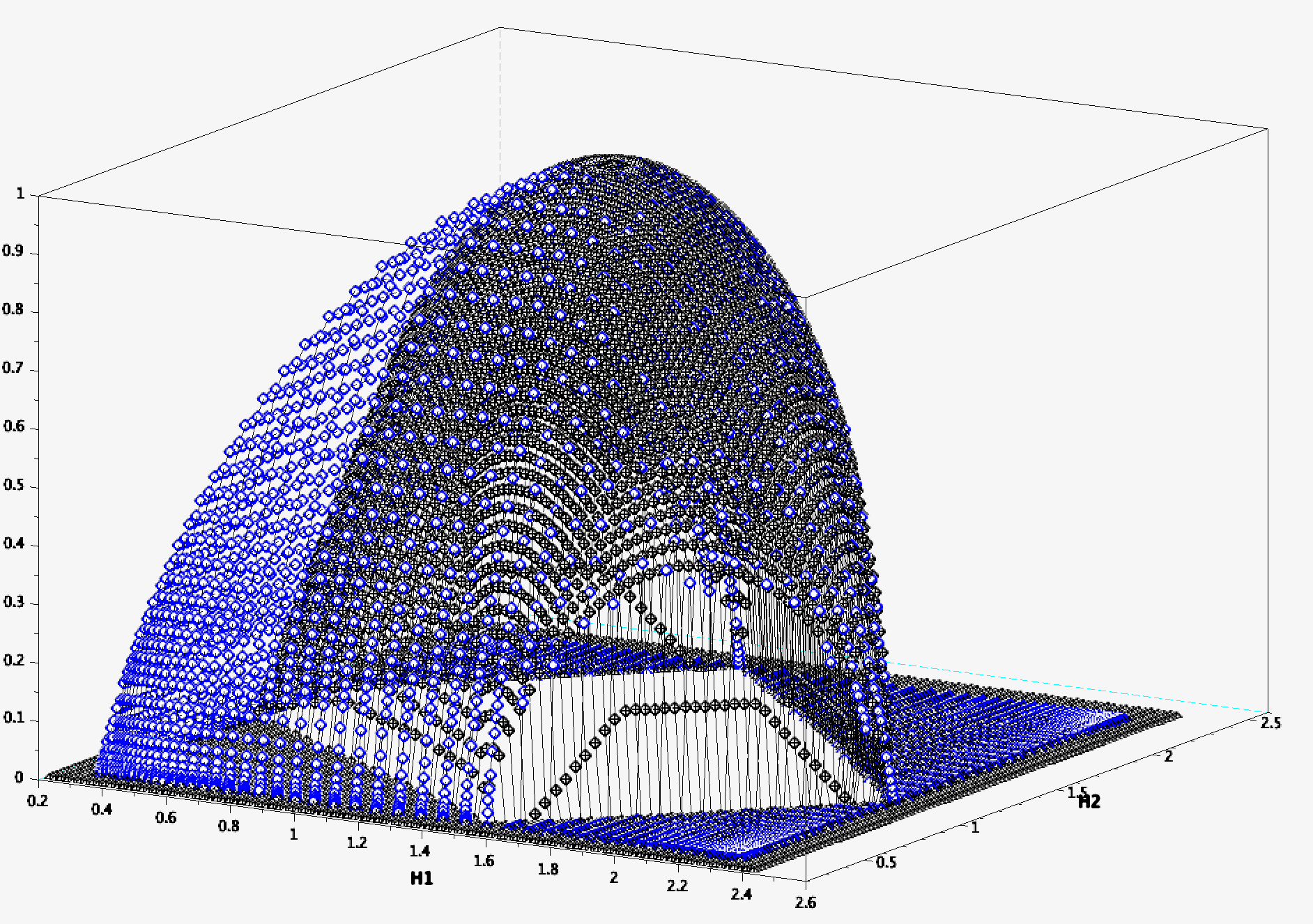
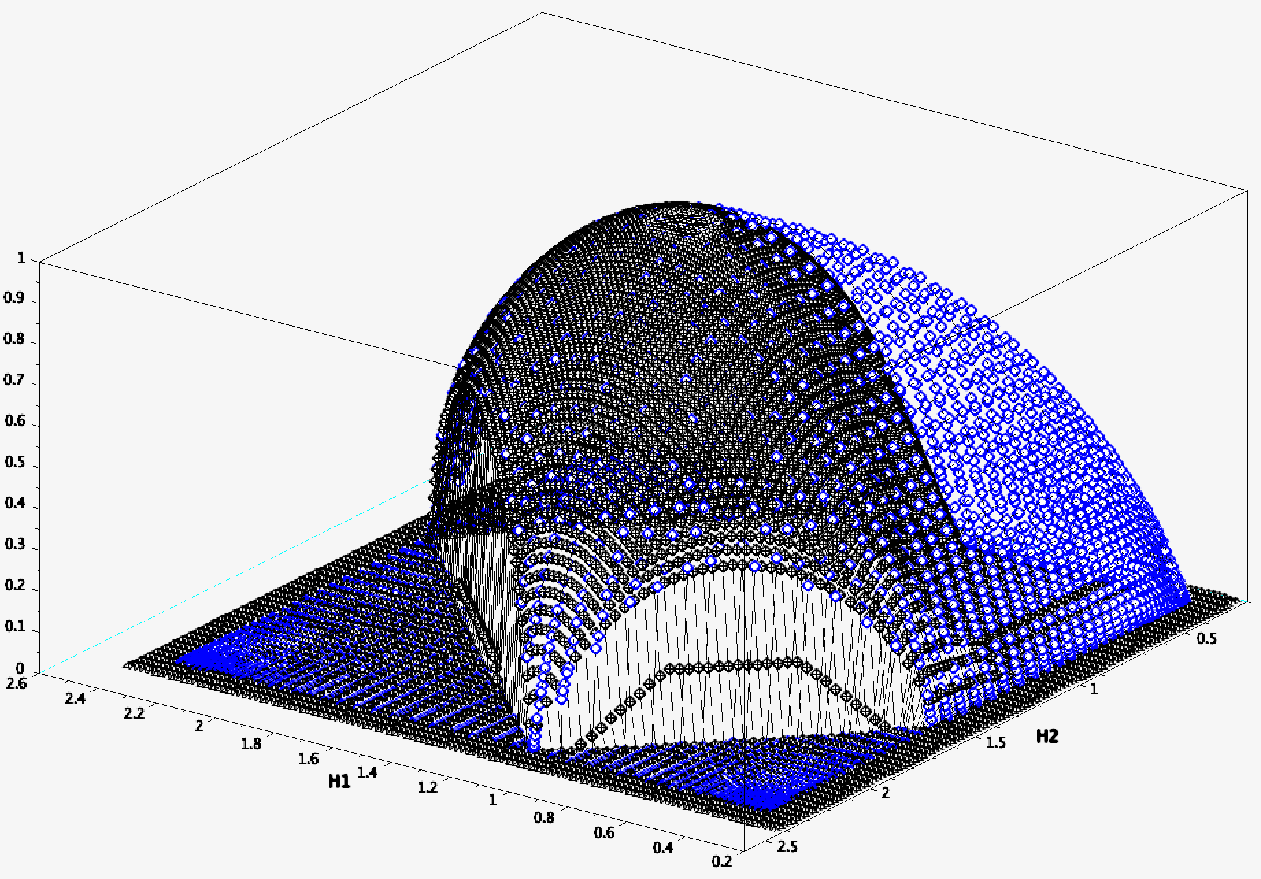
Figure 6. Two views of the superposition of the Legendre (in black) and multifractal (in blue) spectrum of the pair $({\mu_{p_{1}}},\nu_{\eta})$ for $p_{1}=0.2$, $p_{2}=0.8$, $\eta=0.4$. The two spectra coincide on a region of the plane, and $D_{{\mu_{p_{1}}},\nu_{\eta}}$ has a wider support than $\tau_{{\mu_{p_{1}}},\nu_{\eta}}^{*}$.

References

- [1] P. Abry, S. Jaffard, R. Leonarduzzi, S. Seuret, and H. Wendt. Multifractal formalisms for multivariate analysis. Proceedings of the Royal Society A, 2229(475), September 2019.
- [2] N. Attia and J. Barral. Hausdorff and packing spectra, large deviations and free energy for branching random walks in . Comm. Math. Phys., 331(139-187), 2014.
- [3] J. Barral, F. Ben Nasr, and J. Peyrière. Comparing multifractal formalisms: the neighboring condition. Asian J. Math., 7:149–166, 2003.
- [4] J. Barral and D.-J. Feng. On multifractal formalism for self-similar measures with overlaps. Math. Z., 298(1-2):359–383, 2021.
- [5] J. Barral and D.J. Feng. Multifractal formalism for almost all self-affine measures. Comm. Math. Phys., 318:473–504, 2013.
- [6] J. Barral and B. Mandelbrot. Random multiplicative multifractal measures. Proc. Symp. Pure Math., M. L. Lapidus and M. van Frankenhuysen eds, 72:1–52, 2004.
- [7] L. Barreira and B. Saussol. Variational principles and mixed multivariate spectra. Trans. A. M. S., 353 (10):3919–3944, 2001.
- [8] L. Barreira, B. Saussol, and J. Schmeling. Higher-dimensional multifractal analysis. J. Maths Pures Appl., 81:67–91, 2002.
- [9] F. Bayart. Multifractal spectra of typical and prevalent measures. Nonlinearity, 26:353–367, 2013.
- [10] G. Brown, G. Michon, and J. Peyrière. On the multifractal analysis of measures. J. Stat. Phys., 66:775–790, 1992.
- [11] Z. Buczolich and S. Seuret. Typical Borel measures on satisfy a multifractal formalism. Nonlinearity., 23(11):7–13, 2010.
- [12] K. Falconer. Fractal Geometry: Mathematical Foundations and Applications. John Wiley & Sons, West Sussex, England, 1993.
- [13] A.-H. Fan. Multifractal analysis of weighted ergodic averages. Adv. Math., 377, 2021.
- [14] A.-H. Fan, D.-J. Feng, and J.J. Wu. Recurrence, dimension and entropy. J. London Math. Soc., 64:229–244, 2001.
- [15] D.-J. Feng and K.S. Lau. Multifractal formalism for self-similar measures with weak separation condition. J. Math. Pures Appl., 92(3):407–428, 2009.
- [16] D.J. Feng. Gibbs properties of self-conformal measures and the multifractal formalism. Ergodic Theory Dynam. Systems, 27(3):787–812, 2007.
- [17] U. Frisch and D. Parisi. Fully developed turbulence and intermittency in turbulence, and predictability in geophysical fluid dynamics and climate dynamics. International school of Physics “Enrico Fermi”, course 88, edited by M. Ghil, North Holland, pages 84–88, 1985.
- [18] T.C. Halsey, M.H. Jensen, L.P. Kadanoff, I. Procaccia, and B.I. Shraiman. Fractal measures and their singularities: the characterisation of strange sets. Phys. Rev. A, 33:1141–1151, 1986.
- [19] S. Jaffard, S. Seuret, H. Wendt, R. Leonarduzzi, S. Roux, and P. Abry. Multivariate multifractal analysis. Applied and Computational Harmonic Analysis, 46(3):653–663, 2019.
- [20] Zhi-Qiang Jiang, Yan-Hong Yang, Gang-Jin Wang, and Wei-Xing Zhou. Joint multifractal analysis based on wavelet leaders. Frontiers of Physics, 12, 2017.
- [21] K.S. Lau and S.-M. Ngai. Multifractal measures and a weak separation condition. Adv. Math., 141(1):45–96, 1999.
- [22] J.M. Marstrand. Some fundamental geometrical properties of plane sets of fractional dimensions. London Math. Soc. Proc., 3(4):257–302, 1954.
- [23] P. Mattila. Hausdorff dimension, orthogonal projections and intersections with planes. Ann. Acad. Sci. Fenn. Math., 1:227–244, 1975.
- [24] P. Mattila. Geometry of Sets and Measures in Euclidean Spaces. Cambridge University Press, 1995.
- [25] C. Meneveau, K.R. Sreenivasan, P. Kailasnath, and M.S. Fan. Joint multifractal measures - theory and applications to turbulence. Physical Review A, 41(2):894–913, January 1990.
- [26] L. Olsen. A multifractal formalism. Adv. Math., 116:92–195, 1995.
- [27] L. Olsen. Mixed divergence points of self-similar measures. Indiana University Mathematics Journa, 52:1343–1372, 2003.
- [28] L. Olsen. Mixed generalized dimensions of self-similar measures. J. Math. Anal. Appl., 306:516–539, 2005.
- [29] P. Shmerkin. On Furstenberg’s intersection conjecture, self-similar measures, and the norms of convolutions. Ann. Math., 189(2):319–391, 2019.
- [30] H. Wendt, P. Abry, and S. Jaffard. Bootstrap for empirical multifractal analysis. IEEE Signal Process. Mag., 24(4):38–48, 2007.
- [31] M. Wu. A proof of Furstenberg’s conjecture on the intersections of and -invariant sets. Ann. Math., 189(3):707–751, 2019.