Preparation and observation of anomalous counterpropagating edge states in a periodically driven optical Raman lattice

Abstract

Motivated by the recent observation of real-space edge modes with ultracold atoms [Braun et al., Nat. Phys. 20, 1306 (2024)], we investigate the preparation and detection of anomalous counterpropagating edge states—a defining feature of the anomalous Floquet valley-Hall (AFVH) phase—in a two-dimensional periodically driven optical Raman lattice. Modeling the atomic cloud with a Gaussian wave packet state, we explore, both analytically and numerically, how the population of edge modes depends on the initial-state parameters. In particular, we reveal that, in addition to the internal spin state, the initial momenta parallel and perpendicular to the boundary play essential roles: they independently control the selective population of edge states across distinct momenta and within separate quasienergy gaps. Furthermore, we examine the wave-packet dynamics of counterpropagating edge states and demonstrate that their characteristic motion is robust against long-range disorder. These results establish a theoretical framework for future experimental explorations of the AFVH phase and topological phenomena associated with its unique edge modes.

I Introduction

Topological quantum matter has been the focus of intense research over the past decades TI_review1 ; TI_review2 ; Sato2017_review . Central to the discovery of topological materials Konig2007 ; Hsieh2008 ; Xia2009 ; Chang2013 ; Xu2015 ; Lv2015 is the bulk–boundary correspondence Hatsugai1993 ; Qi2006 ; Mong2011 ; Essin2011 , which connects nontrivial bulk topology to the existence of gapless boundary modes. Recently, this foundational principle has been modified and extended to periodically driven systems Rudner2013 ; Nathan2015 . It has been shown that due to the periodicity of quasienergy, traditional topological invariants of Floquet bands, such as the Chern numbers in two-dimensional systems, are insufficient for fully classifying the Floquet topology. Instead, information about edge modes can be derived from the winding numbers defined in the higher momentum-time space, which characterize the topology of the quasienergy gaps Rudner2013 . This new formulation of bulk-boundary correspondence reveals that periodically driven systems can host anomalous edge states and exhibit novel Floquet topological phases that lack static counterparts Kitagawa2010 ; Carpentier2015 ; Fruchar2016 ; Roy2017 ; Yao2017 ; Morimoto2017 ; Huang2023 ; Ghosh2024 .

With their exceptional controllability and cleanliness, ultracold atoms have emerged as an ideal platform for simulating a variety of topological models Goldman2016_review ; Zhang2018_review ; Cooper2019_review ; Schafer2020_review , including the one-dimensional (1D) Su-Schrieffer-Heeger chain Atala2013 , chiral topological phases Song2018 , two-dimensional (2D) Chern insulators Aidelsburger2013 ; Miyake2013 ; Jotzu2014 ; Aidelsburger2015 ; Wu2016 ; Sun2018a ; Liang2023 , and three-dimensional topological semimetals Song2019 ; Wang2021 . These advancements lay a crucial foundation for exploring Floquet topological phases in periodically driven optical lattices Eckardt2017_review ; Rudner2020_review ; Weitenberg2021_review . Recently, several experimental groups have realized anomalous Floquet topological bands Wintersperger2020 ; Lu2022 ; Zhang2023 . Notably, Zhang et al. Zhang2023 successfully manipulated the Floquet band topology by adjusting driving-induced band crossings, unveiling a nontrivial phase known as the anomalous Floquet valley-Hall (AFVH) phase. This phase exhibits protected counterpropagating edge states within each quasienergy gap, eluding classification by conventional global topological invariants Zhang2022 ; Lababidi2014 ; Umer2020 . In their experiment, Zhang et al. identified this unconventional phase using a quench protocol based on local Floquet band structures Zhang2023 ; Zhang2020 ; however, its hallmark feature—the counterpropagating edge states—has yet to be observed, largely due to the challenges associated with creating well-defined boundaries in ultracold atomic gases, necessitating careful preparation and probing techniques for edge modes Stanescu2009 ; Stanescu2010 ; Buchhold2012 ; Goldman2012 ; Goldman2013 ; Reichl2014 ; Goldman2016 ; Leder2016 ; Martinez2023 ; Wang2024 .

Recently, Braun et al. Braun2024 achieved an experimental breakthrough in realizing and observing topological edge modes in real-space Floquet systems. Compared to previous observations in synthetic dimensions Mancini2015 ; Stuhl2015 ; Chalopin2020 , Braun et al. Braun2024 generated and controlled a steep system edge using a programmable repulsive optical potential, and loaded atoms into real-space edge modes by positioning the atomic cloud directly at the edge with an optical tweezer. Upon releasing the atoms, they observed unidirectional wave-packet propagation along the potential boundary, providing clear confirmation of the population of chiral edge modes Martinez2023 ; Braun2024 . This experimental study opens avenues for exploring edge-state dynamics and topological phenomena in real-space platforms.

Inspired by recent experimental advances Zhang2023 ; Braun2024 , we present in this work an analytical and numerical investigation into the preparation and observation of counterpropagating edge states in periodically driven ultracold atoms, providing a direct and explicit approach to identifying the AFVH phase. We analyze how edge-state preparation is influenced by initial-state parameters and find that, in addition to the internal spin state, the momentum of the wave packet plays a crucial role. Specifically, when populating edge modes in the AFVH phase, the initial momentum parallel to the boundary determines which edge state is effectively populated at different momenta, while the initial momentum perpendicular to the boundary serves as a control parameter for selecting edge states within one of the two quasienergy gaps. By preparing an initial state that simultaneously populates two oppositely chiral edge states, we numerically investigate the resulting wave-packet dynamics, which exhibits a counterpropagating motion characteristic of these edge states. Additionally, we demonstrate that the counterpropagating edge-state transport in the AFVH phase remains robust in the presence of long-range disorder. The preparation and detection scheme outlined in this work is well-suited for implementation with current experimental techniques.

This paper is organized as follows. In Sec. II, we introduce the Floquet topological model realized in a 2D shaken optical Raman lattice and analyze its anomalous topological phases. In Sec. III, we demonstrate the method of populating a target edge mode by illustrating how the initial-state parameters, particularly the initial momenta parallel and perpendicular to the boundary, affect the edge-state preparation. In Sec. IV, we investigate the wave-packet transport of counterpropagating edge modes in the AFVH phase and demonstrate their robustness against long-range disorder. A brief discussion and summary are presented in Sec. V. More details are given in the Appendixes.

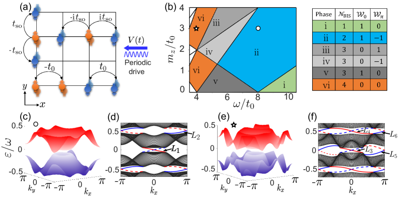
Figure 1: (a) Sketch diagram of the 2D Floquet topological model realized in a shaken optical Raman lattice. (b) Phase diagram as function of the driving frequency $\omega$ and the Zeeman constant $m_{z}$. The Floquet phases can be distinguished by two topological invariants ${\cal W}_{0,\pi}$ combined with the number of BISs ${\cal N}_{\rm BIS}$. Here, we set $t_{\rm so}=0.5t_{0}$ and $V_{0}=3t_{0}$. (c)-(f) Quasienergy band structures with periodic boundary conditions [(c) and (e)] or for a cylindrical geometry [(d) and (f)], corresponding to two phases in (a) labeled by circle ($m_{z}=3t_{0}$, $\omega=8t_{0}$) and star ($m_{z}=3t_{0}$, $\omega=4t_{0}$) markers, respectively. In the open-boundary spectrums [(d) and (f)], edge modes at the left (right) boundary are plotted as solid (dashed) curves, and colored in red (blue) for negative (positive) chirality.

II Model

We consider the Floquet topological system that has been recently realized with ultracold bosons trapped in a shaken optical Raman lattice Zhang2023 , as depicted in Fig. 1(a). The optical Raman lattice scheme has been employed to realize many topological models Song2018 ; Wu2016 ; Sun2018a ; Liang2023 ; Song2019 ; Wang2021 ; Zhang2023 ; LiuXJ2013 ; LiuXJ2014 ; LiuXJ2016 ; ZhangDW2016 ; Lang2017 ; Zhang2017 ; WangBZ2018 ; Yang2018 ; LiuH2019 ; Zheng2019 ; Wang2020 ; Hou2020 ; LuWang2020 ; WangBB2021 ; WangY2022 ; Ziegler2022 ; LiH2023 ; Zhou2023 ; Zhao2023 ; ZhangH2024 ; WangJT2024 . The time-periodic Hamiltonian reads

$$H(t)= -t_{\rm 0}\sum_{\langle{\bf r},{\bf r}^{\prime}\rangle}\left(c^{\dagger}_{{\bf r}\uparrow}c_{{\bf r}^{\prime}\uparrow}-c^{\dagger}_{{\bf r}\downarrow}c_{{\bf r}^{\prime}\downarrow}\right)+\sum_{{\bf r}}\left[m_{z}+V(t)\right]\left(n_{{\bf r}\uparrow}-n_{{\bf r}\downarrow}\right)$$

$$+\sum_{x}\left[\mathbbm{i}t_{\rm{so}}\left(c_{x+1\downarrow}^{\dagger}c_{x\uparrow}-c_{x-1\downarrow}^{\dagger}c_{x\uparrow}\right)+\rm{h.c.}\right]$$

$$+\sum_{y}\left[t_{\rm{so}}\left(c_{y+1\downarrow}^{\dagger}c_{y\uparrow}-c_{y-1\downarrow}^{\dagger}c_{y\uparrow}\right)+\rm{h.c.}\right],$$ (1)

where $c_{{\bf r}\sigma}$ ($c^{\dagger}_{{\bf r}\sigma}$) are the annihilation (creation) operators for spin $\sigma=\uparrow,\downarrow$ at lattice site ${\bf r}=(x,y)$, $n_{{\bf r}\sigma}\equiv c^{\dagger}_{{\bf r}\sigma}c_{{\bf r}\sigma}$, $t_{0}$ ($t_{\rm so}$) denotes the spin-conserved (-flipped) hopping amplitude along the $x$- or $y$-direction, and the periodic drive $V(t)=2V_{0}\cos\omega t$ is applied to the Zeeman term, with $\omega$ being the driving frequency. For simplicity, we set the lattice constant as the unit of length, namely, $a=1$ and assume that the parameters $t_{0}$, $t_{\rm so}$, and $m_{z}$ are all positive. The Bloch Hamiltonian in momentum space takes the form

$$~{}\begin{split}H({\bf k},t)=H_{\rm s}({\bf k})+V(t)\sigma_{z},\quad H_{\rm s}({\bf k})={\bf h}({\bf k})\cdot{\bm{\sigma}},\end{split}$$ (2)

where $\sigma_{x,y,z}$ are the Pauli matrices, and ${\bf h}({\bf k})=(h_{x},h_{y},h_{z})=(2t_{\rm so}\sin k_{x},2t_{\rm so}\sin k_{y},m_{z}-2t_{0}\cos k_{x}-2t_{0}\cos k_{y})$ describes a quantum anomalous Hall model Wu2016 ; Sun2018a . This periodically driven system hosts rich Floquet topological phases beyond conventional classification. The phase diagram as function of $\omega$ and $m_{z}$ is depicted in Fig. 1(b). In the following, we shall review how to characterize the Floquet topology and subsequently apply the approach to analyze anomalous Floquet topological phases.

A Floquet system can be described by an effective Hamiltonian $H_{F}=\mathbbm{i}\log{U(T)}/T$, whose eigenvalues $\varepsilon({\bf k})$ form the Floquet bands with two inequivalent quasienergy gaps Rudner2020_review . Here $T=2\pi/\omega$ is the drive period and $U(T)$ is the time-evolution operator over one period, defined by

$$U(T)={\cal T}e^{-\mathbbm{i}\int_{0}^{T}H(t)dt},$$ (3)

where ${\cal T}$ denotes the time ordering. For a driven system described by Eq. (2), the Floquet Hamiltonian also take a Dirac-type form

$$H_{F}(\mathbb{k})=\sum_{\alpha=x,y,z}h_{F,\alpha}(\mathbb{k})\sigma_{\alpha}.$$ (4)

We adopt the concept of band-inversion surfaces (BISs) and employ the generalized bulk-surface duality to characterize the Floquet topology (see Appendix A and Ref. Zhang2020 for details). Here, for a 2D Floquet system, a BIS refers to a 1D closed curve in the first Brillouin zone where band inversion occurs, i.e.,

$$~{}{\rm BIS}\equiv\{\mathbb{k}|h_{F,z}(\mathbb{k})=0\}.$$ (5)

Unlike static systems, Floquet band crossings can appear at both $\varepsilon=0$ and $\varepsilon=\pi/T$. We name the gap around the quasienergy $0$ ($\pi/T$) as the $0$ gap ($\pi$ gap) and the BIS associated with this gap as $0$ BIS ($\pi$ BIS). Particularly, for the Hamiltonian (2), the definition (5) reduces to $h_{z}(k)=n\omega/2$, where $n=0,1,2,\cdots$, and a 0 BIS ($\pi$ BIS) corresponds to $n$ being even (odd). Hereafter, we will refer to a BIS corresponding to a nonnegative $n$ as the one of order $n$. The Floquet band topology is contributed by all $0$ and $\pi$ BISs Zhang2020 :

$$~{}\mathcal{C}=\mathcal{W}_{0}-\mathcal{W}_{\pi},\quad\mathcal{W}_{q}=\sum_{i}\nu_{i}^{(q)}.$$ (6)

Here $\nu_{i}^{(q)}$ represents the topological invariant defined on the $i$th $q$ BIS ($q=0,\pi$), $\mathcal{C}$ is the Chern number of the Floquet bands, and ${\cal W}_{0}$ (${\cal W}_{\pi}$) characterizes the number of boundary modes inside the 0 gap ($\pi$ gap).

Based on the classification theory presented above, three basic features about the 2D periodical driven cold-atom system have been demonstrated both theoretically Zhang2022 and experimentally Zhang2023 : (i) The two types of BISs—0 BIS and $\pi$ BIS—always appear alternatively. (ii) The topological invariant $\nu_{i}^{(q)}$ can be uniquely determined by the BIS configuration in the first Brillouin zone. Specifically, $\nu_{i}^{(q)}=+1$ ($-1$) when the BIS surrounds the $\Gamma$ ($M$) point. (iii) Each $q$ BIS with $\nu_{i}^{(q)}\neq 0$ ($q=0,\pi$) corresponds to a gapless chiral edge mode within the $q$ gap, rendering the so-called BIS-boundary correspondence Zhang2022 . This correspondence is reflected in the effective subsystem Hamiltonian $H_{\rm eff}^{(n)}({\bf k})=\widetilde{\bf h}({\bf k})\cdot{\bm{\sigma}}$, which is introduced to describe the emergence of a driving-induced BIS of order $n$ (see Appendixes A and B), where $\widetilde{\bf h}({\bf k})=(2\tilde{t}_{\rm so}\sin k_{x},2\tilde{t}_{\rm so}\sin k_{y},\widetilde{m}_{z}-2t_{0}\cos k_{x}-2t_{0}\cos k_{y})$, with

$$\widetilde{m}_{z}=m_{z}-\frac{n\omega}{2},\quad\tilde{t}_{\rm so}=(-1)^{n}J_{n}\left(\frac{4V_{0}}{\omega}\right)t_{\rm so}.$$ (7)

Here $J_{n}(z)$ denotes the Bessel function of the first kind of order $n$. With these three basic features, we can identify two novel Floquet topological phases, as detailed below.

The phase labeled “ii”, characterized by the number of BISs ${\cal N}_{\rm BIS}=2$, is an anomalous phase with a high Chern number ${\cal C}=2$. As illustrated in Fig. 1(c), the quasienergy bands in phase ii exhibit two ring-shaped structures where the band inversion occurs, resulting in two BISs. One is a $0$ BIS circling the $\Gamma$ point, and the other is a $\pi$ BIS circling the $M$ point. According to the feature (ii), we have ${\cal W}_{0}=\nu_{1}^{(0)}=+1$, ${\cal W}_{\pi}=\nu_{1}^{(\pi)}=-1$, and thus ${\cal C}={\cal W}_{0}-{\cal W}_{\pi}=2$. The feature (iii) predicts that there exists a chiral edge mode in either quasienergy gap, which is confirmed by the open-boundary spectrum shown in Fig. 1(d).

The phase labeled “vi” with ${\cal N}_{\rm BIS}=4$ is the AFVH phase, which evades the conventional classification by global topological invariants ${\cal W}_{0,\pi}$ Zhang2022 . The quasienergy band structure shown in Fig. 1(e) indicates the presence of four BISs, of which two are $0$ BISs and two are $\pi$ BISs. Furthermore, the inner $0$ BIS ($\pi$ BIS) circles the $\Gamma$ point, and the outer $0$ BIS ($\pi$ BIS) circles the $M$ point. Based on the BIS circling configuration, we have $\nu_{1}^{(0)}=\nu_{1}^{(\pi)}=+1$ and $\nu_{2}^{(0)}=\nu_{2}^{(\pi)}=-1$, which yields ${\cal W}_{0}=\nu_{1}^{(0)}+\nu_{2}^{(0)}=0$, ${\cal W}_{\pi}=\nu_{1}^{(\pi)}+\nu_{2}^{(\pi)}=0$, and ${\cal C}={\cal W}_{0}-{\cal W}_{\pi}=0$. Despite the trivial bulk topological invariants, the BIS-boundary correspondence ensures the presence of counterpropagating edge modes in both the quasienergy gaps, as illustrated in Fig. 1(f). Although this unconventional phase has been identified through quench-induced spin dynamics Zhang2023 , its unique edge modes have yet to be experimentally observed. In the following sections, we delve into the scheme for preparing and detecting the counterpropagating edge states.

III Edge-state preparation

In this section, we illustrate and numerically demonstrate the method for selectively populating edge modes residing in each of the quasienergy gaps.

III.1 Gaussian wave packet and the internal state

We consider an initial state with a Gaussian spatial distribution centered at $(x_{0},y_{0})$ of width $\delta_{x,y}$:

$$\ket{\Psi_{0}}=\psi_{0}(x,y)\ket{\eta}$$

$$=\frac{1}{\mathcal{N}}\exp[\frac{-(x-x_{0})^{2}}{4\delta_{x}^{2}}+\mathbbm{i}q_{x}x+\frac{-(y-y_{0})^{2}}{4\delta_{y}^{2}}+\mathbbm{i}q_{y}y]\ket{\eta}$$ (8)

where $\mathcal{N}$ denotes the normalization factor and $\ket{\eta}$ is a two-component spinor. The initial momentum $(q_{x},q_{y})$ serves as a control parameter for edge-state preparation, as will be elaborated below. For simplicity, we adopt a cylindrical geometry with periodic boundary conditions in the $x$-direction and open boundary conditions in the $y$-direction, and fix $x_{0}=L/2$ and $y_{0}=1$ throughout this study ($L$ is the lattice size). An example of the wave packet $|\psi_{0}(x,y)|^{2}$ is shown in Fig. 1. While our discussion focuses on the preparation of edge modes at the left boundary, the results can readily be extended to other cases.

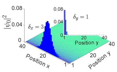
Figure 2: A typical example of the density distribution of the initial state prepared in a $40\times 40$ square lattice with the parameters $(x_{0},y_{0})=(20,1)$ and $(\delta_{x},\delta_{y})=(3,1)$. In our settings, periodic (open) boundary conditions are imposed in the $x$ ($y$)-direction.

We calculate the overlaps $P_{n}=\sum_{x,y}\absolutevalue{\innerproduct{\phi_{n}}{\Psi_{0}}}^{2}$ and investigate the real-space chiral motion of the wave packet to examine the edge-state preparation, where $\ket{\phi_{n}}$ denote the eigenstates of the Floquet Hamiltonian. The time-evolving state at stroboscopic time $t=nT$ ($n\in\mathbb{Z}$) is given by

$$\ket{\Psi(t=nT)}=e^{-\mathbbm{i}H_{F}\cdot nT}\ket{\Psi_{0}}=\begin{pmatrix}\psi_{\uparrow}(x,y,t)\\ \psi_{\downarrow}(x,y,t)\end{pmatrix}.$$ (9)

The wave-packet propagation along the edge can be observed by calculating the distribution at the boundary, i.e.,

$$\absolutevalue{\Psi(x,t)}^{2}\overset{\rm def}{=}\sum_{\sigma=\uparrow,\downarrow}~{}\sum_{y_{\rm edge}}~{}\absolutevalue{\psi_{\sigma}(x,y,t)}^{2},$$ (10)

where $y_{\rm edge}$ denotes the layers at the left boundary, e.g. $y_{\rm edge}=1,2,3,4$ in our calculations.

To effectively populate an edge mode, both the internal spin state and the spatial wave packet should be carefully prepared. Analytical results show that the left edge states take the form

$$\ket{\phi_{L}(k_{x},y)}=\frac{u_{k_{x}}(x)}{\mathcal{N}_{L}}\left(\lambda_{L+}^{y}-\lambda_{L-}^{y}\right)\ket{\eta_{L}},$$ (11)

where $\mathcal{N}_{L}$ denotes the normalization factor, $u_{k_{x}}(x)$ is the Bloch wave function along the $x$-direction, and the complex variables $\lambda_{L\pm}$ are given in Appendix B. The internal state $\ket{\eta_{L}}=\frac{1}{\sqrt{2}}(1,-1)^{\sf T}$ or $\frac{1}{\sqrt{2}}(1,1)^{\sf T}$, depending on the system parameters. Particularly, when $V_{0}/\omega<0.6$, we have a general conclusion (see Appendix B for details)

$$\ket{\eta_{L}}=\left\{\begin{array}[]{ll}\frac{1}{\sqrt{2}}(1,-1)^{\sf T}&\textrm{0-gap edge modes}\\ \frac{1}{\sqrt{2}}(1,1)^{\sf T}&\textrm{$\pi$-gap edge modes}\end{array}\right..$$ (14)

However, it should be noted that the AFVH phase under consideration, marked by a star in Fig. 1(b), is characterized by $V_{0}=3t_{0}$ and $\omega=4t_{0}$, which does not satisfy $V_{0}/\omega<0.6$. Consequently, the left edge mode labeled “$L_{3}$” resides in the 0 gap and possesses the internal state $\ket{\eta_{L}}=\frac{1}{\sqrt{2}}(1,1)^{\sf T}$; other left edge modes are in agreement with the prediction given in Eq. (14) (see Appendix B). The expression (11) indicates that, to populate a desired edge mode, the atoms must be initialized in the appropriate internal state $\ket{\eta}=\ket{\eta_{L}}$. In the following, we assume that this internal state preparation has been successfully achieved via a carefully applied Raman-coupling pulse, which enables control over the population of edge states by finely tuning the wave packet’s momentum $(q_{x},q_{y})$.

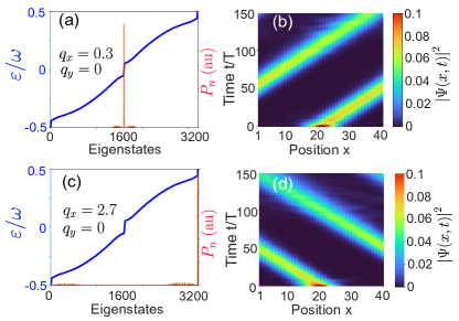
Figure 3: Edge-state preparation in the ${\cal C}=2$ phase, with the two left edge modes $L_{1,2}$, as labeled in Fig. 1(d), being considered. Overlaps of the initial state with Floquet eigenstates $P_{n}$ are shown in (a) and (c), while (b) and (d) illustrate how the initial-state wave packet propagates along the boundary. In (a) and (b), the initial state is prepared in the spin state $\ket{\eta}=\frac{1}{\sqrt{2}}(1,-1)^{\sf T}$ with an initial momentum $(q_{x},q_{y})=(0.3,0)$. In (c) and (d), the initial state is prepared in $\ket{\eta}=\frac{1}{\sqrt{2}}(1,1)^{\sf T}$ with $(q_{x},q_{y})=(2.7,0)$. Here, we take $t_{\rm so}=0.5t_{0}$, $m_{z}=3t_{0}$, $V_{0}=3t_{0}$, $\omega=8t_{0}$, and $(\delta_{x},\delta_{y})=(3,1)$.

III.2 Tuning the initial momentum $(q_{x},q_{y})$

An edge state is characterized by both the momentum $k_{x}$ and the quasienergy gap it resides. We will later demonstrate that the initial momentum $q_{x}$ ($q_{y}$), which is parallel (perpendicular) to the boundary, serves as a control parameter for populating edge modes at different momenta (within distinct gaps). We will examine both the ${\cal C}=2$ phase and the AFVH phase to illustrate it.

As illustrated in Fig. 1(d), the two left edge modes in the ${\cal C}=2$ phase are well separated in momentum $k_{x}$: The edge mode in the 0 gap, labeled “$L_{1}$”, is situated around $k_{x}=0$, while the edge mode in the $\pi$ gap, labeled “$L_{2}$”, emerges around $k_{x}=\pi$. This configuration suggests that an initial kick with varying $q_{x}$ can be employed to control the edge-state preparation. In Fig. 3, we initialize two states that are localized at the center of the edge along the $y$-direction, corresponding to momenta $(q_{x},q_{y})=(0.3,0)$ and $(q_{x},q_{y})=(2.7,0)$, respectively. The overlaps presented in Figs. 3(a) and 3(c) reveal that these initial states are aimed at the edge modes within distinct gaps. Meanwhile, Figs. 3(b) and 3(d) depict the chiral motion of the wave packets, confirming that the edge modes with opposite chirality are effectively populated.

In the AFVH phase, however, two left edge modes residing in different gaps can emerge in the same momentum region. As shown in Fig. 1(f), the edge modes labeled “$L_{3}$” and “$L_{4}$” (“$L_{5}$” and “$L_{6}$” ) are both located around $k_{x}=0$ ($k_{x}=\pi$), and cannot be selectively populated by adjusting the initial momentum $q_{x}$. Surprisingly, we find that the initial momentum perpendicular to the boundary, $q_{y}$, can be employed to effectively control the population of edge states within a specific gap. This finding can be clarified by analyzing the spatial distribution of the edge state phase $\theta(y)$ along the y-direction.

III.2.1 Analytical study

We first consider left edge states at $k_{x}=0$, with the wave-packet function along the $y$-direction taking the form

$$~{}\phi_{L}(y)=\frac{1}{\mathcal{N}_{L}}\left(\lambda_{L+}^{y}-\lambda_{L-}^{y}\right),$$ (15)

where, according to Appendix B,

$$\lambda_{L\pm}=\frac{\widetilde{m}_{z}-2t_{0}\pm\sqrt{\widetilde{m}_{z}^{2}-4t_{0}\widetilde{m}_{z}+4\tilde{t}_{\rm so}^{\,2}}}{2(t_{0}+|\tilde{t}_{\rm so}|)},$$ (16)

and $0<\widetilde{m}_{z}<4t_{0}$. Here, $\widetilde{m}_{z}$ and $\tilde{t}_{\rm so}$ are the parameters of the effective Hamiltonian $H_{\rm eff}^{(n)}({\bf k})$, as presented in Eq. (7). When $\widetilde{m}_{z}^{2}-4t_{0}\widetilde{m}_{z}+4\tilde{t}_{\rm so}^{\,2}<0$, we write $\lambda_{L,\pm}=|\lambda_{L}|e^{\pm\mathbbm{i}\theta_{L}}$, where

$$|\lambda_{L}|=\sqrt{\frac{t_{0}-|\tilde{t}_{\rm so}|}{t_{0}+|\tilde{t}_{\rm so}|}}$$ (17)

and

$$\theta_{L}=\left\{\begin{array}[]{ll}\theta_{L}^{(0)}&2t_{0}\leq\widetilde{m}_{z}<4t_{0}\\ \pi-\theta_{L}^{(0)}&0<\widetilde{m}_{z}<2t_{0}\end{array}\right.,$$ (20)

with $\theta_{L}^{(0)}\equiv\arcsin\left[\sqrt{1-(\widetilde{m}_{z}-2t_{0})^{2}/(4t_{0}^{2}-4\tilde{t}_{\rm so}^{2})}\right]$. With this result, we have

$$~{}\phi_{L}(y)=\frac{2}{\mathcal{N}_{L}}|\lambda_{L}|^{y}\left|\sin(\theta_{L}y)\right|e^{\mathbbm{i}\theta(y)},$$ (21)

with the $y$-dependent phase given by

$$\theta(y) =\frac{\pi}{2}\,{\rm sgn}\left[\sin(\theta_{L}y)\right]$$

$$=\left\{\begin{array}[]{ll}\frac{\pi}{2}\,{\rm sgn}\left[\sin(\theta^{(0)}_{L}y)\right]&2t_{0}\leq\widetilde{m}_{z}<4t_{0}\\ \frac{\pi}{2}\,(-1)^{y+1}{\rm sgn}\left[\sin(\theta^{(0)}_{L}y)\right]&0<\widetilde{m}_{z}<2t_{0}\end{array}\right..$$ (24)

Here, we focus on the two leftmost sites, i.e., $y=1,2$, the spatial distribution at which dominantly determines the overlaps of the initial state with the edge states. We see that when $\theta^{(0)}_{L}<\pi/2$, the phase distribution $\theta(y)$ satisfies

$$\theta(2)=\left\{\begin{array}[]{ll}\theta(1)&2t_{0}<\widetilde{m}_{z}<4t_{0}\\ -\theta(1)&0<\widetilde{m}_{z}<2t_{0}\end{array}\right.,$$ (27)

which means that when $\widetilde{m}_{z}>2t_{0}$ ($\widetilde{m}_{z}<2t_{0}$), the wave-packet function $\phi_{L}(y)$ is symmetrically (antisymmetrically) distributed at the two leftmost sites. Consequently, while an edge state with $\widetilde{m}_{z}>2t_{0}$ can be directly populated without an initial momentum $q_{y}$, a kick with $q_{y}=\pi$ is required to effectively populate an edge state with $\widetilde{m}_{z}<2t_{0}$.

For left edge states at $k_{x}=\pi$, we can draw similar conclusions. The wave-packet function $\phi_{L}(y)$ of an edge state also takes the form of Eq. (15), but with

$$\lambda_{L\pm}=\frac{\widetilde{m}_{z}+2t_{0}\pm\sqrt{\widetilde{m}_{z}^{2}+4t_{0}\widetilde{m}_{z}+4\tilde{t}_{\rm so}^{\,2}}}{2(t_{0}+|\tilde{t}_{\rm so}|)},$$ (28)

and $-4t_{0}<\widetilde{m}_{z}<0$. When $\widetilde{m}_{z}^{2}+4t_{0}\widetilde{m}_{z}+4\tilde{t}_{\rm so}^{\,2}<0$, one can write $\phi_{L}(y)$ in the form of Eq. (21), with the $y$-dependent angle now given by

$$\theta(y)=\left\{\begin{array}[]{ll}\frac{\pi}{2}\,{\rm sgn}\left[\sin(\theta^{(\pi)}_{L}y)\right]&-2t_{0}\leq\widetilde{m}_{z}<0\\ \frac{\pi}{2}\,(-1)^{y+1}{\rm sgn}\left[\sin(\theta^{(\pi)}_{L}y)\right]&-4t_{0}<\widetilde{m}_{z}<-2t_{0}\end{array}\right.,$$ (31)

where $\theta_{L}^{(\pi)}\equiv\arcsin\left[\sqrt{1-(\widetilde{m}_{z}+2t_{0})^{2}/(4t_{0}^{2}-4\tilde{t}_{\rm so}^{2})}\right]$. A similar deduction can be then employed to infer that at $k_{x}=\pi$, an initial kick with $q_{y}=\pi$ is required to populate an edge state with $\widetilde{m}_{z}<-2t_{0}$.

For the AFVH phase, the appearance of four counterpropagating edge modes $L_{3,4,5,6}$, as observed in Fig. 1(f), requires the corresponding Zeeman constants $\widetilde{m}_{z,i}$ ($i=3,4,5,6$) fall into four different ranges, i.e., $4t_{0}>\widetilde{m}_{z,3}>2t_{0}>\widetilde{m}_{z,4}>0>\widetilde{m}_{z,5}>-2t_{0}>\widetilde{m}_{z,6}>-4t_{0}$. This, combined with the above results, shows that the initial momentum $q_{y}$ serves as a control parameter for populating the edge modes of the AFVH phase within different gaps: While the 0-gap edge modes $L_{3,5}$ can be directly populated, an initial kick with $q_{y}=\pi$ is required to effectively populate the edge modes $L_{4,6}$ within the $\pi$ gap.

III.2.2 Numerical demonstration

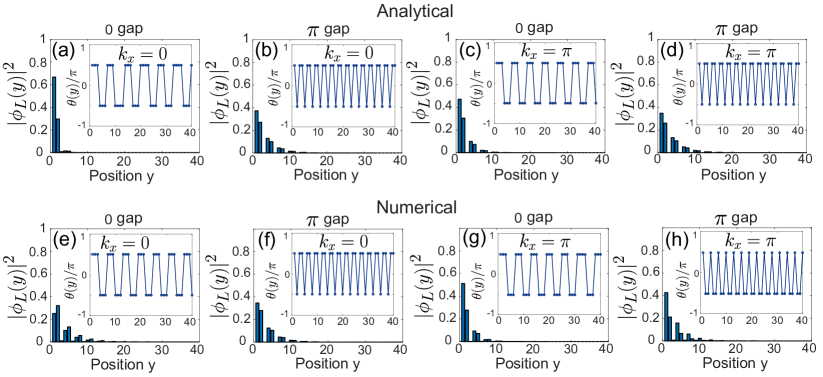
Figure 4: Density distributions $|\phi_{L}(y)|^{2}$ of the left edge states in the AFVH phase, located at $k_{x}=0$ or $\pi$ within the $0$ or $\pi$ gap. For each edge state, the analytical solution (top) is juxtaposed with the corresponding numerical solution (bottom) for a comparison. The inserts show the corresponding phase distributions $\theta(y)$ in the $y$-direction. Here, we take $t_{\rm so}=0.5t_{0}$, $m_{z}=3t_{0}$, $V_{0}=3t_{0}$, and $\omega=4t_{0}$.

To illustrate our analysis, we present in Fig. 4(a)-(d) the analytical solutions for the density distribution $|\phi_{L}(y)|^{2}$ of the left edge states at $k_{x}=0,\pi$ based on Eq. (15), alongside the numerical results in Fig. 4(e)-(h), with the phase distribution $\theta(y)$ displayed in the insets. It is evident that the analytical and numerical solutions are in good agreement. Notably, the 0-gap edge-state wave functions at $k_{x}=0,\pi$ exhibit equal phases at the two leftmost sites, enabling the preparation of a 0-gap edge state without requiring a kick in the $y$-direction. In contrast, the $\pi$-gap edge-state wave functions at $k_{x}=0,\pi$ exhibit a $\pi$-phase jump at the two leftmost sites, indicating that the wave function is distributed nearly antisymmetrically across these two sites; therefore, an initial kick of $q_{y}=\pi$ is necessary to prepare an edge state in the $\pi$ gap.

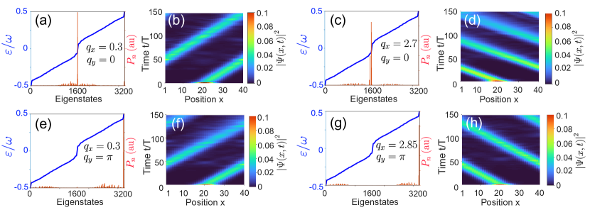
Figure 5: Edge-state preparation in the AFVH phase. The population of the four left edge modes $L_{3,4,5,6}$, as labeled in Fig. 1(f), is considered. Overlaps of the initial state with Floquet eigenstates are shown with the corresponding wave-packet propagation at the boundary. In (a) and (b) [(e) and (f)], the initial state is prepared in the internal spin state $\ket{\eta}=\frac{1}{\sqrt{2}}(1,1)^{\sf T}$ with an initial momentum $(q_{x},q_{y})=(0.3,0)$ [$(0.3,\pi)$]. In (c) and (d) [(g) and (h)], the initial state is prepared in $\ket{\eta}=\frac{1}{\sqrt{2}}(1,-1)^{\sf T}$ [$\frac{1}{\sqrt{2}}(1,1)^{\sf T}$] with an initial momentum $(q_{x},q_{y})=(2.7,0)$ [$(2.85,\pi)$]. Here, we take $t_{\rm so}=0.5t_{0}$, $m_{z}=3t_{0}$, $V_{0}=3t_{0}$, $\omega=4t_{0}$, and $(\delta_{x},\delta_{y})=(3,1)$.

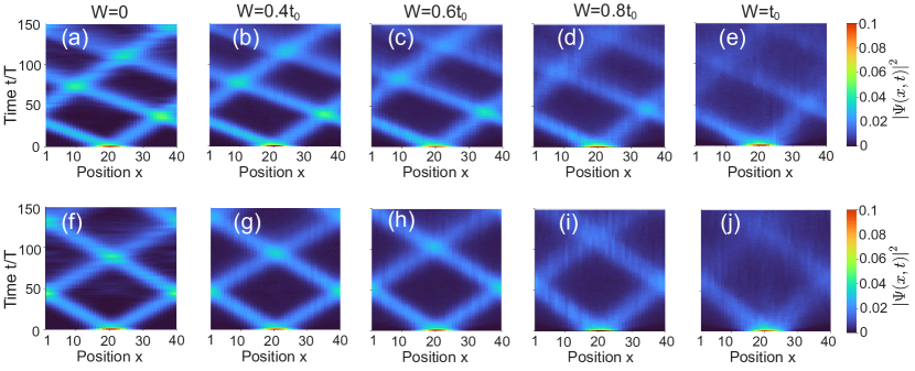
Figure 6: Wave-packet dynamics of counterpropagating edge modes in the 0 gap [(a)-(e)] or $\pi$ gap [(f)-(j)] under the on-site disorder $V_{\rm rand}(\mathbf{r})$, with the disorder strength $W$ ranging from $0$ to $t_{0}$. Other parameters in (a)-(e) [(f)-(j)] are the same as those in Figs. 5(b) and 5(d) [Figs. 5(f) and 5(h)]. Each data point is averaged over 20 disorder configurations.

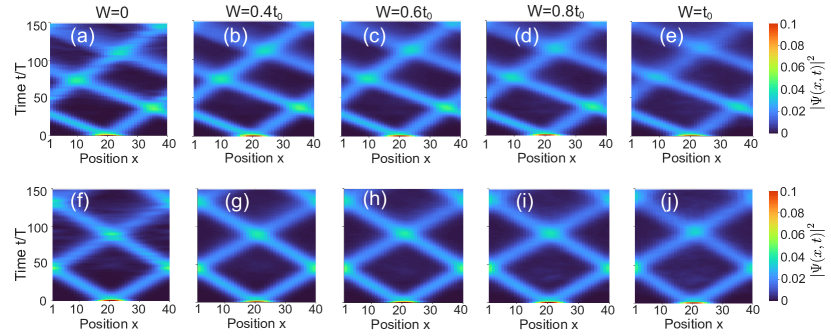
Figure 7: Wave-packet dynamics of counterpropagating edge modes in the 0 gap [(a)-(e)] or $\pi$ gap [(f)-(j)] under the long-range disorder $V_{\rm sm}(\mathbf{r})$, with the disorder strength $W$ ranging from $0$ to $t_{0}$. Other parameters in (a)-(e) [(f)-(j)] are the same as those in Figs. 5(b) and 5(d) [Figs. 5(f) and 5(h)]. Each data point is averaged over 20 disorder configurations.

We investigate the overlaps and the chiral motion of the wave packets to demonstrate edge-state preparation in the same way as in the ${\cal C}=2$ phase. Figures 5(a)-(d) illustrate the initial states prepared in the 0 gap, with Figs. 5(a) and 5(c) showing significant overlaps with the zero quasienergy modes. Figures 5(b) and 5(d) highlight the dynamics of the wave packets, which propagate with opposite chirality, confirming that by adjusting different initial momenta $q_{x}$, the states are effectively prepared to occupy two distinct edge modes $L_{3,5}$ located at $k_{x}=0$ and $\pi$, respectively. Interestingly, Figs. 5(e)-(h) depict the initial states prepared in the $\pi$ gap, which require an initial kick of $q_{y}=\pi$. Figures 5(e) and 5(g) demonstrate that these initial states exhibit strong overlaps with the $\pi$ quasienergy modes, while Figs. 5(f) and 5(h) illustrate the wave packets’ dynamics, once again showing propagation with opposite chirality. This behavior arises from the two different edge modes $L_{4,6}$ being populated through distinct initial momenta $q_{x}$.

Note that the selective population of edge modes within distinct quasienergy gaps relies on the symmetric or antisymmetric distribution of the edge-state wave function at the two leftmost sites, which imposes a constraint on the wave-packet width $\delta_{y}$ of the initial prepared state; specifically, $\delta_{y}$ must not be too small. In practice, $\delta_{y}$ considerably affects edge-state preparation, with an optimal range found to be between 0.7 and 1 (see Appendix C for details).

After demonstrating the effect of the initial momentum $q_{y}$, we now return to the preparation of edge states in the ${\cal C}=2$ phase. The edge mode $L_{2}$ in Fig. 1(d) corresponds to the driving-induced $\pi$ BIS of order $n=1$, for which the effective Hamiltonian is defined with $\widetilde{m}_{z}=m_{z}-\omega/2=-t_{0}$, within the range $-2t_{0}\leq\widetilde{m}_{z}<0$. According to Eq. (31), populating the mode $L_{2}$ does not require a kick in the $y$-direction, consistent with the numerical results shown in Figs. 3(c) and 3(d). However, it is worth noting that for higher driving frequencies, e.g. $\omega>10t_{0}$ for $m_{z}=3t_{0}$, an initial kick of $q_{y}=\pi$ may also be necessary in the preparation of the mode $L_{2}$.

IV Counterpropagating edge-state transport

In this section, we investigate the counterpropagating motion of the oppositely chiral edge states in the AFVH phase, and demonstrate their robustness against long-range disorder. To achieve it, we employ the density matrix to describe the time evolution of the wave packet. The initial density matrix reads

$$\rho(0)=p_{1}\ket{\Psi_{1}}\bra{\Psi_{1}}+p_{2}\ket{\Psi_{2}}\bra{\Psi_{2}}$$ (32)

where $|\Psi_{1,2}\rangle$ are two states taking the form of Eq. (III.1) with different momentum $(q_{x},q_{y})$ and/or internal spin state $\ket{\eta}$, and $p_{1,2}$ are, respectively, the probabilities of the atoms occupying these two states. In our calculations, $p_{1}=p_{2}=0.5$, and the parameters of $|\Psi_{1,2}\rangle$ are chosen to align with those in Fig. 5, ensuring that the initial state can simultaneously populate two counterpropagating edge modes within either the 0 gap or $\pi$ gap. The time evolution at stroboscopic time $t=nT$ ($n\in\mathbb{Z}$) is given by

$$\rho(t=nT)=[U(T)]^{n}\rho(0)[U^{\dagger}(T)]^{n}$$ (33)

where the stroboscopic time-evolution operator $U(T)$ is defined in Eq. (3). Then, the time-dependent density distribution at the boundary can be obtained by

$$\absolutevalue{\Psi(x,t)}^{2}=\sum_{\sigma=\uparrow,\downarrow}~{}\sum_{y_{\rm edge}}\matrixelement{x,y,\sigma}{\rho(t)}{x,y,\sigma},$$ (34)

where $y_{\rm edge}=1,2,3,4$ in our calculations.

Moreover, we examine the robustness of the edge modes’ counterpropagating motion against disorders. We consider two types of disorder potentials applied to the Zeeman term ($m_{z}\rightarrow m_{z}+V_{\rm disorder}$). The first one is random on-site disorder, described by

$$V_{\rm rand}(\mathbf{r})=\sum_{j\in\rm site}V_{j}\delta(\mathbf{r}-\mathbf{r}_{j}).$$ (35)

The second is a long-range potential induced by smooth impurities,

$$V_{\rm sm}(\mathbf{r})=\sum_{l}^{N_{\rm imp}}\frac{V_{l}}{\sqrt{(\mathbf{r}-\mathbf{r}_{l})^{2}+d^{2}}},$$ (36)

where $N_{\rm imp}$ is the number of randomly distributed impurities, $\mathbf{r}_{l}$ denotes the location of $l$th impurity, and $d$ controls the potential range. Here, we restrict $V_{\rm rand},V_{\rm sm}\in[-W,W]$ with $W$ denoting the disorder strength.

In Fig. 6, we present the wave-packet dynamics of the counterpropagating edge modes both within the $0$ gap and $\pi$ gap under random disorder $V_{\rm rand}(\mathbf{r})$ with the strength $W$ ranging from $0$ to $t_{0}$. As the on-site disorder is applied and gradually intensified, we observe a progressive decline in the robustness of the edge transport, indicating that the edge states with opposite chirality are scattering into the bulk. In contrast, Fig. 7 shows that the counterpropagating transport of these edge modes exhibits remarkable robustness against the long-range disorder $V_{\rm sm}(\mathbf{r})$, even as the disorder strength $W$ varies from $0$ to $t_{0}$. This confirms the prediction made in Ref. Zhang2022 that the counterpropagating edge states in the AFVH phase are immune to long-range disorder.

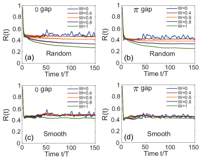
Figure 8: Remnant density $R(t)$ of the wave packet at the boundary as a function of time $t$ under the on-site random disorder $V_{\rm rand}(\mathbf{r})$ [(a) and (b)] or long-range disorder $V_{\rm sm}(\mathbf{r})$ [(c) and (d)]. The results are extracted from the data in Fig. 6 and Fig. 7.

To provide a more detailed analysis, we calculate the remnant density of the wave packet at the boundary and present the results in the Fig. 8. We define $R(t)$ to represent the time-evolving density remaining at the boundary:

$$R(t)=\sum_{x}\absolutevalue{\Psi(x,t)}^{2}.$$ (37)

In Figs. 8(a) and 8(b), we observe that when the on-site random disorder is applied and the disorder strength is increased, the remnant edge-state density decreases. Conversely, in Figs. 8(c) and 8(d), the remnant edge-state density remains nearly constant as the long-range disorder is applied and intensified. These results clearly demonstrate that the counterpropagating edge modes with opposite chirality within the $0$ or $\pi$ gap are robust against long-range disorder, while they are significantly affected by on-site random disorder.

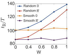
Figure 9: Return time $t_{\rm R}$ of the wave packet prepared in the 0 or $\pi$ gap in the presence of different disorder potentials. The result is extracted from the data in Fig. 6 and Fig. 7.

In addition to the analysis presented above, we offer a complementary perspective to investigate the impact of disorder on the edge-state transport. We introduce a return time $t_{\rm R}$, which quantifies the duration a chiral edge mode propagates along the periodic $x$-direction at the boundary before returning to its initial position. In Fig. 9, we show the return time of the right-propagating wave packet prepared in the 0 or $\pi$ gap, subjected to different disorder potentials. The curves reveal that, with increasing on-site random disorder, the return time $t_{\rm R}$ increases significantly; in contrast, under the smooth disorder, the return time $t_{\rm R}$ remains stable. Thus, on-site disorder impedes the edge-state transport, while smooth disorder has no detrimental effect, reinforcing our earlier conclusion.

V Discussion and conclusions

In this work, we provide a detailed investigation of how to prepare and observe the anomalous counterpropagating edge states with ultracold atoms trapped in a 2D shaken optical Raman lattice. Starting with an initial Gaussian state, we show that both the internal spin state and the wave-packet’s momentum must be carefully prepared to achieve effective population of a target edge state. In particular, in preparing counterpropagating edge states, the population within the 0 gap or $\pi$ gap can be effectively controlled by the application of an initial kick of $\pi$ in the direction perpendicular to the boundary. Furthermore, by examining the wave-packet dynamics, we demonstrate that the counterpropagating edge-state transport is immune to long-range disorder.

The preparation and detection scheme discussed here is readily implementable in current experimental setups. First, a tightly focused optical tweezer can precisely position the atomic cloud at the system edge Braun2024 . Second, the internal spin state of the atoms can be controlled via an appropriately tuned Raman-coupling pulse, while an initial momentum kick can be introduced by shifting the tight trap either parallel or perpendicular to the system edge prior to release. Third, the counterpropagating motion along the edge, observed after releasing the atoms from the trap, can be probed and imaged at a microscopic scale Braun2024 ; Gross2021 , providing high-resolution insights into the edge-state transport. Additionally, disorder potentials can be introduced and finely controlled by projecting laser speckles Lye2005 or by using programmable digital micromirror devices Choi2016 or spatial light modulators White2020 , which offer customizable and tunable disorder landscapes essential for studying disorder effects.

It is worth noting that the AFVH phase exhibits a dependence on edge geometry: for instance, the counterpropagating edge modes within the 0 gap can vanish on zigzag edges when $V_{0}>0.6\omega$ Zhang2022 . In this study, we focus on edge-state transport along a straight edge for simplicity. However, the methods for preparing and observing edge modes discussed here can be readily adapted to other edge geometries. Experimentally, the shape and orientation of the edge can be controlled using a programmable repulsive optical potential Braun2024 , allowing for versatile exploration of geometry-dependent effects in the AFVH phase.

In summary, we have presented a detailed study on the preparation and observation of anomalous counterpropagating edge states with ultracold atoms in a periodically driven optical Raman lattice, establishing a framework for future experimental investigations into the AFVH phase and its unique topological characteristics.

Appendix A Band-inversion surfaces and topological classification theory

In this Appendix, we briefly review the main results of the BIS-based classification theory. More details can be found in Refs. Zhang2018 ; Zhang2019a ; Zhang2019b ; Zhang2020 . For a static system $H_{s}(\mathbb{k})$, the component $h_{z}(\mathbb{k})$ can be chosen to describe the dispersion. The BIS refers to the momenta where band inversion occurs, i.e.,

$$~{}{\rm BIS}\equiv\{\mathbb{k}|h_{z}(\mathbb{k})=0\}.$$ (38)

The remaining components $h_{x,y}(\mathbb{k})$ composes a spin-orbit (SO) field $\mathbb{h}_{\rm so}(\mathbb{k})=(h_{y},h_{x})$, which opens a gap at BISs and leads to nontrivial band topology. According to the bulk-surface duality Zhang2018 , the Chern number that characterizes the bulk topology has a one-to-one correspondence to the 1D winding number defined on all BISs, i.e.,

$$\mathcal{C}=\sum_{i}\nu_{i},$$ (39)

where $\nu_{i}$ counts the winding of the SO field along the $i$th BIS:

$$\nu_{i}=\frac{1}{2\pi}\int_{{\rm BIS}_{j}}d{k_{\parallel}}\left(\hat{h}_{y}\partial_{{k}_{\parallel}}\hat{h}_{x}-\hat{h}_{x}\partial_{{k}_{\parallel}}\hat{h}_{y}\right),$$ (40)

with $k_{\parallel}$ denoting the momentum along the BIS and $\hat{h}_{\alpha}={h}_{\alpha}/\sqrt{h_{x}^{2}+h_{y}^{2}}$ ($\alpha=x,y$).

The above characterization can be generalized to Floquet topological phases Zhang2020 . For the 2D Floquet Hamiltonian taking the form of Eq. (4), one can introduce the BISs of Floquet bands as

$$~{}{\rm BIS}\equiv\{\mathbb{k}|h_{F,z}(\mathbb{k})=0\},$$ (41)

and accordingly define the Floquet SO field $\mathbb{h}_{F,{\rm so}}(\mathbb{k})\equiv(h_{F,y},h_{F,x})$. Due to the periodicity of quasienergy, Floquet band crossings can appear in both the 0 and $\pi$ gaps, and the BISs are determined by Zhang2020

$$h_{z}(k)=n\omega/2,\quad n=0,1,2,\cdots,$$ (42)

where the one of even (odd) order $n$ is the one associated with the 0 gap ($\pi$ gap), named as $0$ BIS ($\pi$ BIS). The topology of the Floquet band below the $0$ gap is contributed by all $0$ and $\pi$ BISs but with opposite signs Zhang2020 :

$$~{}\mathcal{C}=\mathcal{W}_{0}-\mathcal{W}_{\pi},\quad\mathcal{W}_{q}=\sum_{i}\nu_{i}^{(q)},$$ (43)

where ${\cal W}_{0}$ (${\cal W}_{\pi}$) characterizes the number of boundary modes inside the 0 gap ($\pi$ gap) Rudner2013 , and $\nu_{i}^{(q)}$ represents the topological invariant defined on the $i$th $q$ BIS ($q=0,\pi$):

$$\nu_{i}^{(q)}=\frac{1}{2\pi}\int_{q\,{\rm BIS}_{i}}d{k_{\parallel}}\left(\hat{h}_{F,y}\partial_{{k}_{\parallel}}\hat{h}_{F,x}-\hat{h}_{F,x}\partial_{{k}_{\parallel}}\hat{h}_{F,y}\right).$$ (44)

In addition to characterizing the bulk topology, the local topology on each BIS is uniquely linked to the emergence of gapless boundary modes Zhang2022 . It has been shown that a Floquet system can be decomposed into multiple static subsystems, each periodic in quasienergy and composed of bands inverted on a BIS WangBB2024 . For the 2D driven system described by Eq. (2), the subsystem that corresponds to the BIS of order $n$ can be described by the following effective static Hamiltonian Zhang2022

$$~{}H_{\rm eff}^{(n)}=\left(h_{z}-\frac{n\omega}{2}\right)\sigma_{z}+(-1)^{n}J_{n}\left(\frac{4V_{0}}{\omega}\right)(h_{x}\sigma_{x}+h_{y}\sigma_{y}),$$ (45)

where $J_{n}(z)$ denotes the Bessel function of the first kind. This effective Hamiltonian takes the same form as the undriven Hamiltonian $H_{s}$ with the replacements

$$m_{z}\to\widetilde{m}_{z}=m_{z}-\frac{n\omega}{2},$$ (46)

and

$$t_{\rm so}\to\tilde{t}_{\rm so}=(-1)^{n}J_{n}\left(\frac{4V_{0}}{\omega}\right)t_{\rm so},$$ (47)

thus supporting a gapless edge mode when $0<|\widetilde{m}_{z}|<4t_{0}$. This result reveals the one-to-one correspondence between the topology on BISs and gapless edge modes at the boundary. In this work, we employ the effective subsystem Hamiltonian (45) to analyze the driving-induced edge modes.

Appendix B Analytical expressions for chiral edge modes

In this Appendix, we drive analytical expressions for the gapless edge modes in both static and periodically driven systems. We first consider the static Hamiltonian $H_{\rm s}({\bf k})$ and impose open boundary conditions in the $y$-direction. The Hamiltonian can be rewritten as

$$H(k_{x})=\sum_{y}{\cal E}(k_{x})c^{\dagger}_{y}c_{y}+\sum_{y}{\cal T}_{y}c^{\dagger}_{y+1}c_{y}+{\rm h.c.}$$ (48)

where

$${\cal E}(k_{x})=(m_{z}-2t_{0}\cos k_{x})\sigma_{z}+2t_{\rm so}\sin k_{x}\sigma_{x},$$

$${\cal T}_{y}=it_{\rm so}\sigma_{y}-t_{0}\sigma_{z}.$$

We assume that the edge-state wave functions take the form

$$\ket{\phi_{L/R}(k_{x},y)}=\frac{u_{k_{x}}(x)}{\mathcal{N}}\lambda^{y}\ket{\eta_{L/R}},$$ (49)

where $\lambda$ is a complex number, ${\cal N}$ is the normalization factor, $u_{k_{x}}(x)$ denotes the Bloch wave function along the $x$-direction, and $|\eta_{L/R}\rangle$ are two-component spinors. The eigenvalue equation $H(k_{x})\ket{\phi}=E\ket{\phi}$ leads to

$$({\cal T}_{y}^{\dagger}\lambda^{-1}+{\cal E}(k_{x})+{\cal T}_{y}\lambda)\ket{\eta}=E\ket{\eta},$$ (50)

or, in a matrix form,

$$\begin{pmatrix}-2t_{0}\cos k_{x}+m_{z}-\left(\lambda+\lambda^{-1}\right)t_{0}&2t_{\text{so}}\sin k_{x}+\left(\lambda-\lambda^{-1}\right)t_{\text{so}}\\ 2t_{\text{so}}\sin k_{x}+\left(\lambda^{-1}-\lambda\right)t_{\text{so}}&2t_{0}\cos k_{x}-m_{z}+\left(\lambda+\lambda^{-1}\right)t_{0}\end{pmatrix}\begin{pmatrix}\alpha\\ \beta\end{pmatrix}=E\begin{pmatrix}\alpha\\ \beta\end{pmatrix},$$ (51)

which gives the eigenvalues

$$E(k_{x},\lambda)=\pm\sqrt{\left[(m_{z}-2t_{0}\cos k_{x})-t_{0}(\lambda+\lambda^{-1})\right]^{2}+4t_{\rm so}^{2}\sin^{2}k_{x}-t_{\rm so}^{2}(\lambda-\lambda^{-1})^{2}}.$$ (52)

Since $E(k_{x},\lambda)=\pm 2t_{\rm so}\sin k_{x}$ Mong2011 , we have $\left[(m_{z}-2t_{0}\cos k_{x})-t_{0}(\lambda+\lambda^{-1})\right]^{2}-t_{\rm so}^{2}(\lambda-\lambda^{-1})^{2}=0$, which yields four solutions:

$$\begin{split}\lambda_{1\pm}&=\frac{m_{z}-2t_{0}\cos k_{x}\pm\sqrt{\left(m_{z}-2t_{0}\cos k_{x}\right)^{2}-4\left(t_{0}^{2}-t_{\text{so}}^{2}\right)}}{2(t_{0}+t_{\text{so}})},\,{\rm with}\,\ket{\eta_{1}}=\frac{1}{\sqrt{2}}\begin{pmatrix}1\\ -1\end{pmatrix},\,E=-2t_{\rm so}\sin k_{x};\\ \lambda_{2\pm}&=\frac{m_{z}-2t_{0}\cos k_{x}\pm\sqrt{\left(m_{z}-2t_{0}\cos k_{x}\right)^{2}-4\left(t_{0}^{2}-t_{\text{so}}^{2}\right)}}{2(t_{0}-t_{\text{so}})}=1/\lambda_{1\mp},\,{\rm with}\,\ket{\eta_{2}}=\frac{1}{\sqrt{2}}\begin{pmatrix}1\\ 1\end{pmatrix},\,E=2t_{\rm so}\sin k_{x}.\end{split}$$ (53)

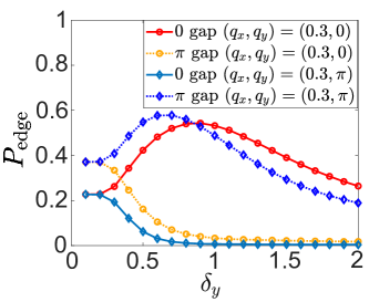
Figure 10: Probability of populating two edge modes $L_{3,4}$ with different wave-packet width $\delta_{y}$. The solid (dashed) lines represent the results of an initial state with momentum $(q_{x},q_{y})=(0.3,0)$ or $(0.3,\pi)$ populating the 0-gap edge mode $L_{3}$ (the $\pi$-gap edge mode $L_{4}$). Other parameters are the same as those in Figs. 5(a) and 5(e).

Since the wavefunctions in Eq. (49) decay (or increase) with $y$ when $|\lambda|<1$ (or $|\lambda|>1$ ), the edge mode localized at the left (right) boundary corresponds to solutions with $|\lambda|<1$ ($|\lambda|>1$). Therefore, the left edge mode takes the form

$$\ket{\phi_{L}(k_{x},y)}=\frac{u_{k_{x}}(x)}{\mathcal{N}_{L}}\left(\lambda_{L+}^{y}-\lambda_{L-}^{y}\right)\ket{\eta_{L}},$$ (54)

where $\lambda_{L\pm}$, with $|\lambda_{L,\pm}|<1$, can be $\lambda_{1\pm}$ or $\lambda_{2\pm}$, which depends on the parameters and also determines the internal state $\ket{\eta_{L}}$. For example, when $m_{z}=3t_{0}$ ($m_{z}=-t_{0}$) and $t_{\rm so}=0.5t_{0}$, there exists a left edge mode around $k_{x}=0$ ($k_{x}=\pi$), which is described by Eq. (54) with $\lambda_{L\pm}=\lambda_{1\pm}$, $\ket{\eta_{L}}=\ket{\eta_{1}}$, and has negative (positive) chirality with $E=-2t_{\rm so}\sin k_{x}$.

We then consider the Floquet Hamiltonian (2). According to the BIS-boundary correspondence established in Ref. Zhang2022 , each 0 or $\pi$ BIS with nontrivial topology corresponds to a chiral edge mode within the corresponding gap. Such a correspondence is reflected in the effective Hamiltonian (45). Consequently, the driving-induced left edge modes also take the form of Eq. (54) with $\lambda_{L\pm}$ being either $\lambda_{1\pm}$ or $\lambda_{2\pm}$ after the replacements specified in Eqs. (46) and (47).

Here, we take the four left edge modes $L_{3,4,5,6}$ in Fig. 1(f) as illustrative examples. The existence of the edge mode $L_{3}$ is ensured by the nonzero topological invariant defined on the static $0$ BIS (the order $n=0$). The effective subsystem Hamiltonian that manifests this BIS-boundary correspondence is then defined with $\widetilde{m}_{z}=m_{z}=3t_{0}$ and $\tilde{t}_{\rm so}=J_{0}\left(3\right)t_{\rm so}\approx-0.26t_{\rm so}$. As a result, the edge mode $L_{3}$ is described by Eq. (54) with $\lambda_{L\pm}=\lambda_{2\pm}$ and $\ket{\eta_{L}}=\ket{\eta_{2}}$. The left edge mode $L_{4}$ corresponds to the driving-induced $\pi$ BIS of order $n=1$, for which $\widetilde{m}_{z}=m_{z}-\omega/2=t_{0}$ and $\tilde{t}_{\rm so}=-J_{1}\left(3\right)t_{\rm so}\approx-0.34t_{\rm so}$. This results in the left edge mode $L_{4}$ being located around $k_{x}=0$ within the $\pi$ gap and taking the form of Eq. (54) also with $\lambda_{L\pm}=\lambda_{2\pm}$ and $\ket{\eta_{L}}=\ket{\eta_{2}}$. The left edge mode $L_{5}$ corresponds to the $0$ BIS of order $n=2$; the parameters $\widetilde{m}_{z}=m_{z}-\omega=-t_{0}$ and $\tilde{t}_{\rm so}=J_{2}\left(3\right)t_{\rm so}\approx 0.49t_{\rm so}$ determine that $L_{5}$ is located around $k_{x}=\pi$ within the $0$ gap and exhibits a distribution characterized by $\lambda_{L\pm}=\lambda_{1\pm}$ and $\ket{\eta_{L}}=\ket{\eta_{1}}$. The left edge mode $L_{6}$ corresponds to the $\pi$ BIS of order $n=3$; the parameters $\widetilde{m}_{z}=m_{z}-3\omega/2=-3t_{0}$ and $\tilde{t}_{\rm so}=-J_{3}\left(3\right)t_{\rm so}\approx-0.31t_{\rm so}$ lead to $L_{6}$ distributed around $k_{x}=\pi$ within the $\pi$ gap, with $\lambda_{L\pm}=\lambda_{2\pm}$ and $\ket{\eta_{L}}=\ket{\eta_{2}}$. The above analytical predictions agree with the numerical results.

Moreover, it is noteworthy that when the driving strength is relatively weak, $V_{0}<0.6\omega$, ensuring $J_{n}\left(\frac{4V_{0}}{\omega}\right)>0$ for all $n\leq 0$, the sign of the parameter $\tilde{t}_{\rm so}$ depends solely on the order $n$ [cf. Eq. (47)]. When $n$ is even, we have $\tilde{t}_{\rm so}>0$ and the solutions with $|\lambda|<1$ can only be $\lambda=\lambda_{1\pm}$ with the spin state $\ket{\eta_{1}}$. In contrast, when $n$ is odd, we have $\tilde{t}_{\rm so}<0$ and the solutions with $|\lambda|<1$ are $\lambda=\lambda_{2\pm}$ with the spin state $\ket{\eta_{2}}$. This leads to the general conclusion presented in Eq. (14).

Appendix C The dependence of edge-state preparation on the width $\delta_{y}$

Throughout the main text, the wave-packet width is fixed at $\delta_{y}=1$. In this Appendix, we investigate how varying the width $\delta_{y}$ affects the preparation of edge states. To this end, we calculate the total probability of the prepared initial state populating the target edge mode $L_{i}$ by

$$P_{\rm edge}=\sum_{n\in L_{i}}\sum_{x,y}|\innerproduct{\phi_{n}}{\Psi_{0}}|^{2},$$ (55)

where $\ket{\phi_{n}}$ denote the eigenstates of the edge mode $L_{i}$ and $\ket{\Psi_{0}}$ is the initial state taking the form of Eq. (III.1).

We revisit the preparation of the edge modes $L_{3,4}$ shown in Figs. 5(a) and 5(e), and present the calculated probability $P_{\rm edge}$ in Fig. 10, where the width $\delta_{y}$ is varied from 0.1 to 2. We find that (i) the probability of populating the target edge modes $L_{3,4}$ depends on the width $\delta_{y}$, with an optimal range between 0.7 and 1; and (ii) the momentum $q_{y}$ can effectively control the population of the edge mode within the 0 or $\pi$ gap, requiring the width $\delta_{y}>0.6$. This second result is consistent with our analysis, in which it is the wave-function distribution at the two leftmost sites that results in the selective population via an initial kick $q_{y}$.

References

- (1) M. Z. Hasan and C. L. Kane, Colloquium: Topological insulators, Rev. Mod. Phys. 82, 3045 (2010).
- (2) X.-L. Qi and S.-C. Zhang, Topological insulators and superconductors, Rev. Mod. Phys. 83, 1057 (2011).
- (3) M. Sato and Y. Ando, Topological superconductors: a review, Rep. Prog. Phys. 80, 076501 (2017).
- (4) M. König, S. Wiedmann, C. Brüne, A. Roth, H. Buhmann, L. W. Molenkamp, X.-L. Qi, and S.-C. Zhang, Quantum spin Hall insulator state in HgTe quantum wells, Science 318, 766 (2007).
- (5) D. Hsieh, D. Qian, L. Wray, Y. Xia, Y. S. Hor, R. J. Cava, and M. Z. Hasan, A topological Dirac insulator in a quantum spin Hall phase, Nature (London) 452, 970 (2008).
- (6) Y. Xia, D. Qian, D. Hsieh, L. Wray, A. Pal, H. Lin, A. Bansil, D. Grauer, Y. S. Hor, R. J. Cava, and M. Z. Hasan, Observation of a large-gap topological-insulator class with a single Dirac cone on the surface, Nat. Phys. 5, 398 (2009).
- (7) C.-Z. Chang, J. Zhang, X. Feng, J. Shen, Z. Zhang, M. Guo, K. Li, Y. Ou, P. Wei, L.-L. Wang, Z.-Q. Ji, Y. Feng, S. Ji, X. Chen, J. Jia, X. Dai, Z. Fang, S.-C. Zhang, K. He, Y. Wang, L. Lu, X.-C. Ma, and Q.-K. Xue, Experimental observation of the quantum anomalous Hall effect in a magnetic topological insulator, Science 340, 167 (2013).
- (8) S. Y. Xu, I. Belopolski, N. Alidoust, M. Neupane, G. Bian, C. L. Zhang, R. Sankar, G. Q. Chang, Z. J. Yuan, C. C. Lee, S. M. Huang, H. Zheng, J. Ma, D. S. Sanchez, B. K. Wang, A. Bansil, F. C. Chou, P. P. Shibayev, H. Lin, S. Jia, and M. Z. Hasan, Discovery of a Weyl fermion semimetal and topological Fermi arcs, Science 349, 613 (2015).
- (9) B. Q. Lv, H. M. Weng, B. B. Fu, X. P. Wang, H. Miao, J. Ma, P. Richard, X. C. Huang, L. X. Zhao, G. F. Chen, Z. Fang, X. Dai, T. Qian, and H. Ding, Experimental Discovery of Weyl Semimetal TaAs, Phys. Rev. X 5, 031013 (2015).
- (10) Y. Hatsugai, Chem Number and Edge States in the Integer Quantum Hall Effect, Phys. Rev. Lett. 71, 3697 (1993).
- (11) X.-L. Qi, Y.-S. Wu, and S.-C. Zhang, General theorem relating the bulk topological number to edge states in two-dimensional insulators, Phys. Rev. B 74, 045125 (2006).
- (12) R. S. K. Mong and V. Shivamoggi, Edge states and the bulk-boundary correspondence in Dirac Hamiltonians, Phys. Rev. B 83, 125109 (2011).
- (13) A. M. Essin and V. Gurarie, Bulk-boundary correspondence of topological insulators from their respective Green’s functions, Phys. Rev. B 84, 125132 (2011).
- (14) M. S. Rudner, N. H. Lindner, E. Berg, and M. Levin, Anomalous Edge States and the Bulk-Edge Correspondence for Periodically Driven Two-Dimensional Systems, Phys. Rev. X 3, 031005 (2013).
- (15) F. Nathan and M. S. Rudner, Topological singularities and the general classification of Floquet-Bloch systems, New J. Phys. 17, 125014 (2015).
- (16) T. Kitagawa, E. Berg, M. Rudner, and E. Demler, Topological characterization of periodically driven quantum systems, Phys. Rev. B 82, 235114 (2010).
- (17) D. Carpentier, P. Delplace, M. Fruchart, and K. Gawedzki, Topological Index for Periodically Driven Time-Reversal Invariant 2D Systems, Phys. Rev. Lett. 114, 106806 (2015).
- (18) M. Fruchart, Complex classes of periodically driven topological lattice systems, Phys. Rev. B 93, 115429 (2016).
- (19) R. Roy and F. Harper, Periodic table for Floquet topological insulators, Phys. Rev. B 96, 155118 (2017).
- (20) S. Yao, Z. Yan, and Z. Wang, Topological invariants of Floquet systems: General formulation, special properties, and Floquet topological defects, Phys. Rev. B 96, 195303 (2017).
- (21) T. Morimoto, H. C. Po, and A. Vishwanath Floquet topological phases protected by time glide symmetry, Phys. Rev. B 95, 195155 (2017).
- (22) B. Huang, Topological invariants for anomalous Floquet higher-order topological insulators. Front. Phys. 18, 13601 (2023).
- (23) A. K. Ghosh, T. Nag, and A. Saha, Generation of higher-order topological insulators using periodic driving, J. Phys.: Condens. Matter 36 093001 (2024).
- (24) N. Goldman, J. C. Budich, and P. Zoller, Topological quantum matter with ultracold gases in optical lattices, Nat. Phys. 12, 639 (2016).
- (25) D.-W. Zhang, Y.-Q. Zhu, Y. X. Zhao, H. Yan, S.-L. Zhu, Topological quantum matter with cold atoms, Adv. Phys. 67, 253 (2018).
- (26) N. R. Cooper, J. Dalibard, and I. B. Spielman, Topological bands for ultracold atoms, Rev. Mod. Phys. 91, 015005 (2019).
- (27) F. Schäfer, T. Fukuhara, S. Sugawa, Y. Takasu, and Y. Takahashi, Tools for quantum simulation with ultracold atoms in optical lattices, Nat. Rev. Phys. 2, 411 (2020).
- (28) M. Atala, M. Aidelsburger, J. T. Barreiro, D. Abanin, T. Kitagawa, E. Demler, and I. Bloch, Direct measurement of the Zak phase in topological Bloch bands, Nat. Phys. 9, 795 (2013).
- (29) B. Song, L. Zhang, C. He, T. F. J. Poon, E. Hajiyev, S. Zhang, X.-J. Liu, and G.-B. Jo, Observation of symmetry-protected topological band with ultracold fermions, Sci. Adv. 4, eaao4748 (2018).
- (30) M. Aidelsburger, M. Atala, M. Lohse, J. T. Barreiro, B. Paredes, and I. Bloch, Realization of the Hofstadter Hamiltonian with Ultracold Atoms in Optical Lattices, Phys. Rev. Lett. 111, 185301 (2013).
- (31) H. Miyake, G. A. Siviloglou, C. J. Kennedy, W. C. Burton, and W. Ketterle, Realizing the Harper Hamiltonian with LaserAssisted Tunneling in Optical Lattices, Phys. Rev. Lett. 111, 185302 (2013).
- (32) G. Jotzu, M. Messer, R. Desbuquois, M. Lebrat, T. Uehlinger, D. Greif, and T. Esslinger, Experimental realization of the topological Haldane model with ultracold fermions, Nature (London) 515, 237 (2014).
- (33) M. Aidelsburger, M. Lohse, C. Schweizer, M. Atala, J. T. Barreiro, S. Nascimbène, N. R. Cooper, I. Bloch, and N. Goldman, Measuring the Chern number of Hofstadter bands with ultracold bosonic atoms, Nat. Phys. 11, 162 (2015).
- (34) Z. Wu, L. Zhang, W. Sun, X. Xu, B. Wang, S. Ji, Y. Deng, S. Chen, X. Liu, and J.-W. Pan, Realization of two-dimensional spin-orbit coupling for Bose-Einstein condensates, Science, 354, 83 (2016).
- (35) W. Sun, B.-Z. Wang, X.-T. Xu, C.-R. Yi, L. Zhang, Z. Wu, Y. Deng, X.-J. Liu, S. Chen, and J.-W. Pan, Highly Controllable and Robust 2D Spin-Orbit Coupling for Quantum Gases, Phys. Rev. Lett. 121, 150401 (2018).
- (36) M.-C. Liang, Y.-D. Wei, L. Zhang, X.-J. Wang, H. Zhang, W.-W. Wang, W. Qi, X.-J. Liu, and X. Zhang, Realization of Qi-Wu-Zhang model in spin-orbit-coupled ultracold fermions, Phys. Rev. Research 5, L012006 (2023).
- (37) B. Song, C. He, S. Niu, L. Zhang, Z. Ren, X.-J. Liu, and G.-B. Jo, Observation of nodal-line semimetal with ultracold fermions in an optical lattice, Nat. Phys. 15, 911 (2019).
- (38) Z. Wang, X. Cheng, B. Wang, J. Zhang, Y. Lu, C. Yi, S. Niu, Y. Deng, X. Liu, S. Chen, and J.-W. Pan, Realization of an ideal Weyl semimetal band in a quantum gas with 3D spin-orbit coupling, Science, 372, 271. (2021).
- (39) A. Eckardt, Colloquium: Atomic quantum gases in periodically driven optical lattices, Rev. Mod. Phys. 89, 011004 (2017).
- (40) M. S. Rudner and N. H. Lindner, Band structure engineering and non-equilibrium dynamics in Floquet topological insulators. Nat. Rev. Phys. 2, 229 (2020).
- (41) C. Weitenberg and J. Simonet, Tailoring quantum gases by Floquet engineering, Nat. Phys. 17, 1342 (2021).
- (42) K. Wintersperger, C. Braun, F. N. Ünal, A. Eckardt, M. D. Liberto, N. Goldman, I. Bloch and M. Aidelsburger, Realization of an anomalous Floquet topological system with ultracold atoms, Nat. Phys. 16, 1058 (2020).
- (43) M. Lu, G. H. Reid , A. R. Fritsch , A. M. Piñeiro, and I. B. Spielman, Floquet Engineering Topological Dirac Bands, Phys. Rev. Lett. 129, 040402 (2022).
- (44) J.-Y. Zhang, C.-R. Yi, L. Zhang, R.-H. Jiao, K.-Y. Shi, H. Yuan, W. Zhang, X.-J. Liu, S. Chen, and J.-W. Pan, Tuning Anomalous Floquet Topological Bands with Ultracold Atoms, Phys. Rev. Lett. 130, 043201 (2023).
- (45) L. Zhang and X.-J. Liu, Unconventional Floquet Topological Phases from Quantum Engineering of Band-Inversion Surfaces, PRX Quantum 3, 040312 (2022).
- (46) M. Lababidi, I. I. Satija, and E. Zhao, Counter-propagating Edge Modes and Topological Phases of a Kicked Quantum Hall System, Phys. Rev. Lett. 112, 026805 (2014).
- (47) M. Umer, R. W. Bomantara, and J. Gong, Counterpropagating edge states in Floquet topological insulating phases Phys. Rev. B 101, 235438 (2020).
- (48) L. Zhang, L. Zhang, and X.-J. Liu, Unified Theory to Characterize Floquet Topological Phases by Quench Dynamics, Phys. Rev. Lett. 125, 183001 (2020).
- (49) T. D. Stanescu, V. Galitski, J. Y. Vaishnav, C. W. Clark, and S. D. Sarma, Topological insulators and metals in atomic optical lattices, Phys. Rev. A 79, 053639 (2009).
- (50) T. D. Stanescu, V. Galitski, and S. D. Sarma, Topological states in two-dimensional optical lattices, Phys. Rev. A 82, 013608 (2010).
- (51) M. Buchhold, D. Cocks, and W. Hofstetter, Effects of smooth boundaries on topological edge modes in optical lattices, Phys. Rev. A 85, 063614 (2012).
- (52) N. Goldman, J. Beugnon, and F. Gerbier, Detecting Chiral Edge States in the Hofstadter Optical Lattice, Phys. Rev. Lett. 108, 255303 (2012).
- (53) N. Goldman, J. Dalibard, A. Dauphin, F. Gerbier, M. Lewenstein, P. Zoller, and I. B. Spielman, Direct imaging of topological edge states in cold-atom systems, Proc. Natl. Acad. Sci. USA 110, 6736 (2013).
- (54) M. D. Reichl and E. J. Mueller, Floquet edge states with ultracold atoms, Phys. Rev. A 89, 063628 (2014).
- (55) N. Goldman, G. Jotzu, M. Messer, F. Görg, R. Desbuquois, and T. Esslinger, Creating topological interfaces and detecting chiral edge modes in a two-dimensional optical lattice, Phys. Rev. A 94, 043611 (2016).
- (56) M. Leder, C. Grossert, L. Sitta, M. Genske, A. Rosch, and M. Weitz, Real-space imaging of a topologically protected edge state with ultracold atoms in an amplitude-chirped optical lattice, Nat. Commun. 7, 13112 (2016).
- (57) M. F. Martínez and F. N. Ünal, Wave-packet dynamics and edge transport in anomalous Floquet topological phases, Phys. Rev. A 108, 063314 (2023).
- (58) B. Wang, M. Aidelsburger, J. Dalibard, A. Eckardt, and N. Goldman, Cold-Atom Elevator: From Edge-State Injection to the Preparation of Fractional Chern Insulators, Phys. Rev. Lett. 132, 163402 (2024).
- (59) C. Braun, R. Saint-Jalm, A. Hesse, J. Arceri, I. Bloch, and M. Aidelsburger, Real-space detection and manipulation of topological edge modes with ultracold atoms, Nat. Phys. 20, 1306 (2024).
- (60) M. Mancini, G. Pagano, G. Cappellini, L. Livi, M. Rider, J. Catani, C. Sias, P. Zoller, M. Inguscio, M. Dalmonte, and L. Fallani, Observation of chiral edge states with neutral fermions in synthetic Hall ribbons, Science 349, 1510 (2015).
- (61) B. K. Stuhl, H.-I. Lu, L. M. Aycock, D. Genkina, and I. B. Spielman, Visualizing edge states with an atomic Bose gas in the quantum Hall regime, Science 349, 1514 (2015).
- (62) T. Chalopin, T. Satoor, A. Evrard, V. Makhalov, J. Dalibard, R. Lopes, and S. Nascimbene, Probing chiral edge dynamics and bulk topology of a synthetic Hall system, Nat. Phys. 16, 1017 (2020).
- (63) X.-J. Liu, Z.-X. Liu, and M. Cheng, Manipulating Topological Edge Spins in a One-Dimensional Optical Lattice, Phys. Rev. Lett. 110, 076401 (2013).
- (64) X.-J. Liu, K. T. Law, and T. K. Ng, Realization of 2D Spin-Orbit Interaction and Exotic Topological Orders in Cold Atoms, Phys. Rev. Lett. 112, 086401 (2014).
- (65) X.-J. Liu, Z.-X. Liu, K. T. Law, W. V. Liu, and T. K. Ng, Chiral topological orders in an optical Raman lattice, New J. Phys. 18 035004 (2016).
- (66) D.-W. Zhang, Y. X. Zhao, R.-B. Liu, Z.-Y. Xue, S.-L. Zhu, and Z. D. Wang, Quantum simulation of exotic -invariant topological nodal loop bands with ultracold atoms in an optical lattice, Phys. Rev. A 93, 043617 (2016).
- (67) L.-J. Lang, S.-L. Zhang, and Q. Zhou, Nodal Brillouin-zone boundary from folding a Chern insulator, Phys. Rev. A 95, 053615 (2017).
- (68) S.-L. Zhang and Q. Zhou, Two-leg Su-Schrieffer-Heeger chain with glide reflection symmetry, Phys. Rev. A 95, 061601(R) (2017).
- (69) B.-Z. Wang, Y.-H. Lu, W. Sun, S. Chen, Y. Deng, and X.-J. Liu, Dirac-, Rashba-, and Weyl-type spin-orbit couplings: Toward experimental realization in ultracold atoms, Phys. Rev. A 97, 011605(R) (2018).
- (70) Y.-B. Yang, L.-M. Duan, and Y. Xu, Continuously tunable topological pump in high-dimensional cold atomic gases, Phys. Rev. B 98, 165128 (2018).
- (71) H. Liu, T.-S. Xiong, W. Zhang, and J.-H. An, Floquet engineering of exotic topological phases in systems of cold atoms, Phys. Rev. A 100, 023622 (2019).
- (72) Z. Zheng, Z. Lin, D.-W. Zhang, S.-L. Zhu, and Z. D. Wang, Chiral magnetic effect in three-dimensional optical lattices, Phys. Rev. Research 1, 033102 (2019).
- (73) Y. Wang, L. Zhang, S. Niu, D. Yu, and X.-J. Liu, Realization and Detection of Nonergodic Critical Phases in an Optical Raman Lattice, Phys. Rev. Lett. 125, 073204 (2020).
- (74) J. Hou, H. Hu, and C. Zhang, Topological phases in pseudospin-1 Fermi gases with two-dimensional spin-orbit coupling, Phys. Rev. A 101, 053613 (2020).
- (75) Y.-H. Lu, B.-Z. Wang, X.-J. Liu, Ideal Weyl semimetal with 3D spin-orbit coupled ultracold quantum gas, Sci. Bull. 65, 2080 (2020).
- (76) B.-B. Wang, J.-H. Zhang, C. Shan, F. Mei, and S. Jia, Topological nodal chains in optical lattices, Phys. Rev. A 103, 033316 (2021).
- (77) Y. Wang, Mobility edges and critical regions in a periodically kicked incommensurate optical Raman lattice, Phys. Rev. A 106, 053312 (2022).
- (78) L. Ziegler, E. Tirrito, M. Lewenstein, S. Hands, and A. Bermudez, Correlated Chern insulators in two-dimensional Raman lattices: A cold-atom regularization of strongly coupled four-Fermi field theories, Phys. Rev. Research 4, L042012 (2022).
- (79) H. Li and W. Yi, Dissipative two-dimensional Raman lattice, Phys. Rev. A 107, 013306 (2023).
- (80) X.-C. Zhou, T.-H. Yang, Z.-Y. Wang, X.-J. Liu, Non-Abelian dynamical gauge field and topological superfluids in optical Raman lattice, arXiv:2309.12923.
- (81) E. Zhao, Z. Wang, C. He, T. F. J. Poon, K. K. Pak, Y.-J. Liu, P. Ren, X.-J. Liu, and G.-B. Jo, Two-dimensional non-Hermitian skin effect in an ultracold Fermi gas, arXiv:2311.07931.
- (82) H. Zhang, W.-W. Wang, C. Qiao, L. Zhang, M.-C. Liang, R. Wu, X.-J. Wang, X.-J. Liu, and X. Zhang, Topological spin-orbit-coupled fermions beyond rotating wave approximation, Sci. Bull. 69 747 (2024).
- (83) J.-T. Wang, J.-X. Liu, H.-T. Ding, and P. He, Proposal for implementing Stiefel-Whitney insulators in an optical Raman lattice, Phys. Rev. A 109, 053314 (2024).
- (84) C. Gross and W. S. Bakr, Quantum gas microscopy for single atom and spin detection, Nat. Phys. 17, 1316 (2021).
- (85) J. E. Lye, L. Fallani, M. Modugno, D. S. Wiersma, C. Fort, and M. Inguscio, Bose-Einstein Condensate in a Random Potential, Phys. Rev. Lett. 95, 070401 (2005).
- (86) J.-Y. Choi, S. Hild, J. Zeiher, P. Schauß, A. Rubio-Abadal, T. Yefsah, V. Khemani, D. A. Huse, I. Bloch, and C. Gross, Exploring the many-body localization transition in two dimensions, Science 352, 1547 (2016).
- (87) D. H. White, T. A. Haase, D. J. Brown, M. D. Hoogerland, M. S. Najafabadi, J. L. Helm, C. Gies, D. Schumayer, and D. A. W. Hutchinson, Observation of two-dimensional Anderson localisation of ultracold atoms, Nat. Commun. 11, 4942 (2020).
- (88) L. Zhang, L. Zhang, S. Niu, and X.-J. Liu, Dynamical classification of topological quantum phases, Sci. Bull. 63, 1385 (2018).
- (89) L. Zhang, L. Zhang, and X.-J. Liu, Dynamical detection of topological charges, Phys. Rev. A 99, 053606 (2019).
- (90) L. Zhang, L. Zhang, and X.-J. Liu, Characterizing topological phases by quantum quenches: A general theory, Phys. Rev. A 100, 063624 (2019).
- (91) B.-B. Wang and L. Zhang, Characterizing Floquet topological phases by quench dynamics: A multiple-subsystem approach, Phys. Rev. A 109, 023303 (2024)