Robust Data-Driven Predictive Control for Mixed Platoons under Noise and Attacks

Abstract

Controlling mixed platoons, which consist of both connected and automated vehicles (CAVs) and human-driven vehicles (HDVs), poses significant challenges due to the uncertain and unknown human driving behaviors. Data-driven control methods offer promising solutions by leveraging available trajectory data, but their performance can be compromised by process noise and adversarial attacks. To address this issue, this paper proposes a Robust Data-EnablEd Predictive Leading Cruise Control (RDeeP-LCC) framework based on data-driven reachability analysis. The framework over-approximates system dynamics under noise and attack using a matrix zonotope set derived from data, and develops a stabilizing feedback control law. By decoupling the mixed platoon system into nominal and error components, we employ data-driven reachability sets to recursively compute error reachable sets that account for noise and attacks, and obtain tightened safety constraints of the nominal system. This leads to a robust data-driven predictive control framework, solved in a tube-based control manner. Numerical simulations and human-in-the-loop experiments validate that the RDeeP-LCC method significantly enhances the robustness of mixed platoons, improving mixed traffic stability and safety against practical noise and attacks.

I Introduction

Recent advancements in connected and automated vehicles (CAVs) have led to the increasing deployment of vehicles featuring various levels of autonomous driving capabilities. Among these innovations, adaptive cruise control (ACC) has emerged as a significant implementation, reducing the need for constant driver intervention in speed management [1] and enhancing proactive driving safety [2]. Despite these benefits, recent empirical and experimental studies [3, 4] have revealed the inherent limitations of ACC in optimizing traffic flow. These limitations are primarily attributed to ACC’s over-conservative car-following policy and short-sighted perception capabilities [5].

In contrast to ACC, cooperative adaptive cruise control (CACC) employs vehicle-to-vehicle (V2V) communication to organize multiple CAVs as a pure CAV platoon and apply cooperative control methods. This approach shows substantial potential in improving traffic performance, including traffic stability [6], road capacity [7], and energy efficiency [8]. However, the effectiveness of CACC is hindered by the requirement for all the involved vehicles to possess autonomous capabilities. A mixed traffic environment, characterized by the coexistence of CAVs and human-driven vehicles (HDVs), is anticipated to persist for an extended period. In the near future, particularly at low CAV penetration rates, the probability of consecutive vehicles being equipped with CAV technology becomes negligible [9, 10]. To overcome the limitations of pure CAV platoons in mixed traffic, mixed platooning has emerged as a promising alternative, which integrates both CAVs and HDVs in a vehicle platoon [11, 12, 13]. The core idea is to guide the behavior of HDVs by directly controlling CAVs, thereby enhancing overall traffic performance [14, 15]. Recent studies, including traffic simulations [16, 17], hardware-in-the-loop tests [18, 19], and real-world experiments [14, 20], have shown the potential benefits of mixed platoons for smoothing traffic flow and improving traffic efficiency, even at low CAV penetration rates.

To achieve these benefits while preserving CAV safety, existing research on mixed platoon control mainly relies on model-based control methods. These methods utilize microscopic car-following models, such as the intelligent driver model (IDM) [21] and optimal velocity model (OVM) [22], to capture the longitudinal behavior of HDVs. Parametric models are then derived to represent the dynamics of the entire mixed platoon system, enabling the implementation of various model-based control strategies, including linear quadratic regulator [11], structured optimal control [15], model predictive control (MPC) [23], $\mathcal{H}_{\infty}$ robust control [24], and control barrier function [25]. However, the inherent randomness and uncertainty in the car-following behavior of HDVs present a significant challenge in accurately identifying the mixed platoon dynamics. The resulting model mismatches may limit the performance of these model-based techniques. On the other hand, model-free or data-driven methods have gained increasing attention [26, 27, 28, 29]. Approaches like adaptive dynamic programming [26, 27] and reinforcement learning [28, 16] have shown potential in learning CAV control policies through iterative training, without the necessity of a previous knowledge about the dynamics of mixed platoons. However, it is worth noting that safety is always prioritized first for CAVs, but these methods lack principled safety constraints, as they typically take an indirect manner by penalizing unsafe actions in the reward function. Although recent advancements, such as safe reinforcement learning, have begun to formally address safety concerns in mixed platoons [30, 31], these methods still face significant challenges, including high computational demands and limited generalization capabilities.

For deriving safe and optimal control inputs directly from data, one promising approach is data-driven predictive control, with the combination of the well-established MPC and data-driven techniques [32]. Along this direction, several methods have been proposed for data-driven mixed platoon control [33, 34, 35], with a notable example being Data-EnablEd Predictive Control (DeePC) [36]. Specifically, DeePC represents the system behavior in a data-centric manner via Willems’ fundamental lemma [37], and incorporates explicit input-output constraints in online predictive control optimization. By adapting DeePC to a Leading Cruise Control (LCC) framework [38], which is particularly designed for mixed traffic, the recently proposed Data-EnablEd Predictive Leading Cruise Control (DeeP-LCC) allows for CAVs’ safe and optimal control in mixed platoons [34]. The effectiveness of this approach has been validated across multiple dimensions, including the mitigation of traffic waves [34], the reduction of energy consumption [39], and the enhancement of privacy protection [40]. However, real-world data are always corrupted by noise from vehicle perception systems or V2X communication channels. Moreover, these data-driven CAV control systems become increasingly vulnerable to attacks in the V2X network, which may maliciously alter control inputs or perceived data to execute attacks [41], thereby compromising CAV control safety. Existing research tends to overlook the influence of noise on data collection and online predictive control, and often assumes the absence of adversarial attacks. This assumption could limit the CAV’s ability to effectively follow desired trajectories and may raise significant safety concerns [42].

To explicitly address noise and attacks, growing evidence has indicated that robustness is crucial in standard DeePC [43, 44]. Indeed, a recent paper has reformulated DeeP-LCC using min-max robust optimization to handle unknown disturbances [45]. However, prior assumptions on disturbances are still needed to improve computational efficiency. Compared to the min-max approach, reachability analysis offers a more computationally reliable method for ensuring robustness against a wide range of noise and attacks. Several recent works have applied similar techniques to design robust control strategies for CAVs, including anti-attack control employing reach-avoid specification [41] and formal safety net control using backward reachability analysis [46]. Note that most of these methods are model-based, with one notable exception of [33], which presents a data-driven reachability analysis approach. Nonetheless, the prediction accuracy in [33] may be limited by the utilization of over-approximated data-driven dynamics. Moreover, the boundaries of noise and attack have not been well-explored in [33], which could significantly affect the performance of data-driven predictive control.

To address the aforementioned research gaps, this paper proposes a Robust Data-EnablEd Predictive Leading Cruise Control (RDeeP-LCC) method that leverages data-driven reachability analysis. The goal is to develop robust data-driven control strategies for CAVs against noise and attacks in mixed platoons. We introduce specific evaluation indices to comprehensively analyze RDeeP-LCC’s tracking performance under different boundary conditions. Additionally, human-in-the-loop experiments are conducted to provide near-real-world validation. Some preliminary results have been outlined in [47]. Precisely, the main contributions of this paper are as follows:

• We propose a novel RDeeP-LCC formulation for mixed platoon control that explicitly addresses process noise and adversarial attacks. Inspired by [33, 48], we capture process noise and adversarial attacks as zonotope sets, in contrast to the zero assumption in [34]. We decouple the system into nominal and error subsystems and use matrix zonotope set techniques to build an over-approximated error reachable set. By subtracting this set from the system constraints, we derive a tightened nominal reachable set, which is used as a safety constraint to reformulate the standard DeeP-LCC problem. The nominal control input is computed accordingly, and the actual control input for the CAV is obtained via a tube-based control manner, combining nominal and error feedback control inputs to enhance safety and robustness.

• We then perform numerical simulations to compare the control performance of RDeeP-LCC with baseline methods, including standard MPC and standard DeeP-LCC. Specifically, our analysis focuses on quantifying the impact of varying noise and attack boundaries on platoon tracking performance. The simulation results show that, without explicitly addressing noise and adversarial attacks, standard DeeP-LCC performs even worse than traditional HDV-only traffic. In contrast, the proposed RDeeP-LCC consistently outperforms the baseline methods under various noise and attack boundary conditions, demonstrating its significant robustness improvements for data-driven control techniques in mixed traffic systems.

• Finally, human-in-the-loop experiments are conducted with real human drivers engaged using driving simulators, whereas existing research primarily relies on simulations with HDVs represented by recorded data or car-following models. Results show that standard DeeP-LCC fails to stabilize mixed traffic under noise and attack conditions. By contrast, RDeeP-LCC outperforms the baseline methods, achieving a $26.1\text{\,}\%$ reduction in velocity deviations and a $24.7\text{\,}\%$ decrease in real cost, compared to all-HDV traffic, while standard MPC exhibits smaller reductions of $18.8\text{\,}\%$ and $16.5\text{\,}\%$, respectively. These results highlight the superior robustness and practical effectiveness of RDeeP-LCC in smoothing traffic flow against common noise and adversarial attacks.

The remainder of this paper is organized as follows: Section II introduces the problem statement and preliminaries. Section III presents the RDeeP-LCC formulation. Section IV shows numerical simulations. Human-in-the-loop experiments are provided in Section V, and Section VI concludes this paper.

II Problem Statement

In this section, we first introduce the research scenario, and then give the parametric model of the mixed platoon system under the LCC framework [38]. The parametric model is commonly employed in model-based methods, which serve as a baseline for our proposed data-driven approach.

II-A Research Scenario

We consider a mixed platoon system comprising one leading CAV (indexed as $1$) and $n-1$ following HDVs (indexed as $2,\ldots,n$ against the moving direction), as shown in Figure 1. Define an index set $\Omega=\{1,2,\ldots,n\}$ encompassing the indices of all vehicles within the mixed platoon. The sets of CAV indices and HDV indices are denoted by $\Omega_{\mathrm{C}}=\{1\}$ and $\Omega_{\mathrm{H}}=\{2,\ldots,n\}$, respectively. All vehicles in the mixed platoon follow a head vehicle (HV) (indexed as $0$), which is immediately ahead of the CAV. This mixed platoon system has been called the Leading Cruise Control (LCC) in [38], and could be regarded as the minimum subsystem structure for the entire mixed traffic flow.

In this study, we consider a centralized control framework, which could be deployed in an edge cloud control platform. Precisely, we assume that roadside units can acquire state data for all the vehicles in the mixed platoon and transmit it to the cloud control platform without delay. Then, a specific controller within the cloud calculates the control commands, which are sent to the CAVs to regulate mixed platoons.

It is worth noting that for platoon control, a small variation in the velocity of the head vehicle could necessitate a corresponding and synchronized adjustment in the velocity for all subsequent vehicles to maintain operational safety. Given the fact that only the CAV is under direct control in mixed platoons, the dynamic process of velocity adaptation poses substantial challenges, particularly in scenarios where the system is subject to process noise and adversarial attacks. Under such conditions, the effective control of CAVs becomes crucial to ensure the safety and stability of the entire mixed platoon. Accordingly, the main research focus of this paper is to develop a robust data-driven control framework for CAVs that can effectively mitigate the impact of process noise and adversarial attacks. Particularly, as shown in Fig. 1, we assume that the noise affects the observation process of the system state in the cloud control platform, while the attacks deceive or inject the control input received by the CAVs.

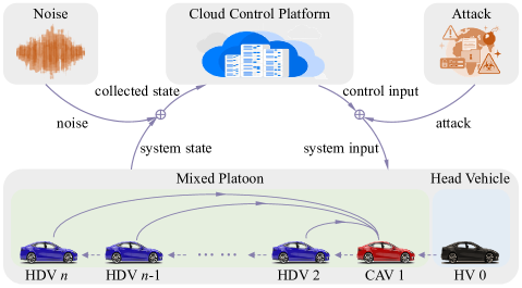
Figure 1: Schematic for mixed platoon under the influence of noise and attacks. The blue, red, and black vehicles are HDVs, CAV, and head vehicle, respectively. The blue and green boxes represent the head vehicle and mixed platoon, respectively. The noise and attacks affect the uplink and downlink of the cloud control platform, respectively.

II-B Parametric Model of Mixed Platoon System

In the following, we introduce the parametric modeling process for mixed platoons, which is commonly used in model-based methods. For all vehicles $i\in\Omega$, a second-order model is used to describe the longitudinal dynamics, given by [11, 23, 15]

$$\begin{cases}\dot{p}_{i}(t)=v_{i}(t),\\ \dot{v}_{i}(t)=u_{i}(t),\end{cases}\quad i\in\Omega$$ (1)

where $p_{i}(t)$, $v_{i}(t)$, and $u_{i}(t)$ denote the position, velocity, and control input of the vehicle $i$, respectively.

For HDVs, the control input $u_{i}(t)$ in (1) is influenced by driver behavior, and several established car-following models, such as OVM [22] and IDM [21], provide specific formulations for this input. Particularly, the general expression of $u_{i}(t)$ can be written as follows:

$$u_{i}(t)=F_{i}(s_{i}(t),\dot{s}_{i}(t),v_{i}(t)),\quad i\in\Omega_{\mathrm{H}},$$ (2)

where $s_{i}(t)=p_{i-1}(t)-p_{i}(t)$ and $\dot{s}_{i}(t)=v_{i-1}(t)-v_{i}(t)$ denote the spacing and relative velocity between vehicle $i$ and its preceding vehicle $i-1$, respectively, and $F_{i}(\cdot)$ denotes the general car-following function.

Define spacing error $\tilde{s}_{i}(t)$ and velocity error $\tilde{v}_{i}(t)$ to indicate the deviations of spacing and velocity from their respective equilibrium states, as follows:

$$\begin{cases}\tilde{s}_{i}(t)={s}_{i}(t)-s^{*}_{i},\\ \tilde{v}_{i}(t)={v}_{i}(t)-v^{*}_{i},\end{cases}\quad i\in\Omega$$ (3)

where $s^{*}_{i}$ and $v^{*}_{i}$ represent the equilibrium spacing and velocity, which satisfy the condition $F(s^{*}_{i},0,v^{*}_{i})=0$.

By applying the first-order Taylor expansion on (2) at the equilibrium state $(s^{*}_{i},v^{*}_{i})$ and combining it with (1) to derive the linearized model for the HDVs, we have:

$$\begin{cases}\dot{\tilde{s}}_{i}(t)=\tilde{v}_{i-1}(t)-\tilde{v}_{i}(t),\\ \dot{\tilde{v}}_{i}(t)=\gamma_{i,1}\tilde{s}_{i}(t)+\gamma_{i,2}\tilde{v}_{i}(t)+\gamma_{i,3}\tilde{v}_{i-1}(t),\end{cases}\quad i\in\Omega_{\mathrm{H}}$$ (4)

where $\gamma_{i,1}=\frac{\partial F_{i}}{\partial s_{i}}$, $\gamma_{i,2}=\frac{\partial F_{i}}{\partial{\dot{s}_{i}}}-\frac{\partial F_{i}}{\partial{v}_{i}}$, and $\gamma_{i,3}=\frac{\partial F_{i}}{\partial\dot{s}_{i}}$ denote the linearized coefficients for $\tilde{s}_{i}(t)$, $\tilde{v}_{i}(t)$, and $\tilde{v}_{i-1}(t)$ from (2) at equilibrium state $(s^{*}_{i},v^{*}_{i})$. It is important to note that for realistic driving characteristics, the coefficients $\gamma_{i,1}$, $\gamma_{i,2}$, $\gamma_{i,3}$ must satisfy the conditions $\gamma_{i,1}>0$ and $\gamma_{i,2}>\gamma_{i,3}>0$.

For the CAVs, we assume that the control input is attacked, similar to the HDVs model (4), the linearized longitudinal dynamics can be expressed in the following form:

$$\begin{cases}\dot{\tilde{s}}_{i}(t)=\tilde{v}_{i-1}(t)-\tilde{v}_{i}(t),\\ \dot{\tilde{v}}_{i}(t)=u_{i}(t)+\vartheta(t),\end{cases}\quad i\in\Omega_{\mathrm{C}}$$ (5)

where $u_{i}(t)$ is the designed control input for CAVs, and $\vartheta(t)$ captures the adversarial attacks for control input, the model setting of such attack information has already existed in [41, 49].

We define $x_{i}(t)=\left[\tilde{s}_{i}(t),\tilde{v}_{i}(t)\right]^{\top}$ as the state vector for vehicle $i$ in the mixed platoon, and lump the states of all vehicles to obtain the mixed platoon system state $x(t)=\left[x_{1}^{\top}(t),x_{2}^{\top}(t),\ldots,x_{n}^{\top}(t)\right]^{\top}\in\mathbb{R}^{2n\times 1}$. Combining (4) and (5), and taking into account noise, the state-space model of the mixed platoon is obtained as:

$$\dot{x}(t)=A_{\rm{con}}x(t)+B_{\rm{con}}u(t)+H_{\rm{con}}\epsilon(t)+J_{\rm{con}}\vartheta(t)+\omega(t),$$ (6)

where $A_{\rm{con}}\in\mathbb{R}^{2n\times 2n}$ represents the system matrix, $B_{\rm{con}}\in\mathbb{R}^{2n\times 1}$ denotes the control matrix, $H_{\rm{con}}\in\mathbb{R}^{2n\times 1}$ represents the disturbance input matrix, $J\in\mathbb{R}^{2n\times 1}$ denotes the attack input matrix, $u(t)\in\mathbb{R}$ represents the control input for the CAV. We denote $\epsilon(t)=\tilde{v}_{0}(t)\in\mathbb{R}$ as the velocity deviation of the head vehicle, and $\omega(t)\in\mathbb{R}^{2n\times 1}$ as the unknown but bounded noise. The matrices $A_{\rm{con}}$, $B_{\rm{con}}$, $H_{\rm{con}}$, and $J_{\rm{con}}$ are defined as follows respectively:

$$\begin{bmatrix}A_{1}&&&&&\\ D_{2}&A_{2}&&&&\\ &\ddots&\ddots&&&\\ &&D_{i}&A_{i}&&\\ &&&\ddots&\ddots&\\ &&&&D_{n}&A_{n}\end{bmatrix},\\ \begin{bmatrix}B_{1}\\ B_{2}\\ \vdots\\ B_{i}\\ \vdots\\ B_{n}\end{bmatrix},\begin{bmatrix}H_{1}\\ H_{2}\\ \vdots\\ H_{i}\\ \vdots\\ H_{n}\end{bmatrix},\begin{bmatrix}J_{1}\\ J_{2}\\ \vdots\\ J_{i}\\ \vdots\\ J_{n}\end{bmatrix},$$ (7)

with sub-block matrices within (7) is given as follows:

$$\begin{array}[]{l}A_{1}=\begin{bmatrix}0&-1\\ 0&0\end{bmatrix},A_{i}=\begin{bmatrix}0&-1\\ \gamma_{i,1}&-\gamma_{i,2}\end{bmatrix},D_{i}=\begin{bmatrix}0&1\\ 0&\gamma_{i,3}\end{bmatrix},\\ B_{1}=\begin{bmatrix}0\\ 1\end{bmatrix},B_{i}=\begin{bmatrix}0\\ 0\end{bmatrix},H_{1}=\begin{bmatrix}1\\ 0\end{bmatrix},H_{i}=\begin{bmatrix}0\\ 0\end{bmatrix},\\ J_{1}=\begin{bmatrix}0\\ 1\end{bmatrix},J_{i}=\begin{bmatrix}0\\ 0\end{bmatrix},i\in\Omega_{\mathrm{H}}.\end{array}$$ (8)

Subsequently, the continuous system in (6) can be discretized employing the forward Euler method, taking into account process noise, resulting in the discrete model for the mixed platoon system:

$${x}(k+1)=Ax(k)+Bu(k)+H\epsilon(k)+J\vartheta(k)+\omega(k),$$ (9)

where $k$ represents the discrete time step, $A$, $B$, $H$, and $J$ are the system matrix, control input matrix, disturbance input matrix, and attack input matrix of the discrete system with appropriate dimensions. Motivated by the existing research [41, 49], we assume that the disturbance $\epsilon(k)$, the attack $\vartheta(k)$, and the noise $\omega(k)$ are norm bounded, given by

$$\left\|\epsilon(k)\right\|_{\infty}\leq\epsilon_{\mathrm{max}},\quad\left\|\vartheta(k)\right\|_{\infty}\leq\vartheta_{\mathrm{max}},\quad\left\|\omega(k)\right\|_{\infty}\leq\omega_{\mathrm{max}},$$ (10)

where $\epsilon_{\mathrm{max}}$, $\vartheta_{\mathrm{max}}$, and $\omega_{\mathrm{max}}$ are the upper bounds of $\epsilon(k)$, $\vartheta(k)$, and $\omega(k)$, respectively.

Remark 1

Although the typical car-following models can capture the longitudinal driving behavior of human drivers, human’s uncertain and unknown nature makes it non-trivial to accurately identify the model (9) involving particular HDVs. Accordingly, the system matrices $A$, $B$, $H$, and $J$ are uncertain and unknown, which motivates us to develop a data-driven predictive control method to obtain the optimal control input $u(k)$ for CAVs. Note that the model (9), which is indeed unknown, is only used to clarify the dimensions and physical meaning of state and control variables in this paper, facilitating our design of the data-driven dynamics and reachability analysis in Section III.

II-C Preliminaries and Theoretical Foundations

Before proceeding, we present the necessary preliminaries on reachable sets and data-driven predictive control. For clarity, we may slightly abuse some notations, which will be used exclusively in this subsection.

We first define set representations to be used in the reachable set computation. Note that the state dimension of a mixed platoon system increases as the platoon size $n$ grows up, which significantly raises the computational complexity of typical reachable set methods. Motivated by [48], we utilize zonotope sets to describe the reachable sets for efficient computation. Some basic definitions are as follows.

Definition 1 (Interval Set [50])

An interval set $\mathcal{I}$ is a connected subset of $\mathbb{R}^{n}$, and it can be defined as $\mathcal{I}=\left\{x_{\mathcal{I}}\in\mathbb{R}^{n}\mid\underline{x}_{\mathcal{I}_{i}}\leq x_{\mathcal{I}_{i}}\leq\overline{x}_{\mathcal{I}_{i}}\quad\forall i=1,\cdots,n\right\}$, where $\underline{x}_{\mathcal{I}_{i}}$ and $\overline{x}_{\mathcal{I}_{i}}$ are the lower bound and upper bound of $x_{\mathcal{I}_{i}}$, respectively. Interval set can be represented as $\mathcal{I}=[\underline{\mathcal{I}},\overline{\mathcal{I}}]$, with $\underline{\mathcal{I}}=[\underline{x}_{\mathcal{I}_{1}},\underline{x}_{\mathcal{I}_{2}},\cdots,\underline{x}_{\mathcal{I}_{n}}]$ and $\overline{\mathcal{I}}=[\overline{x}_{\mathcal{I}_{1}},\overline{x}_{\mathcal{I}_{2}},\cdots,\overline{x}_{\mathcal{I}_{n}}]$.

Definition 2 (Zonotope Set [51])

Given a center vector $c_{\mathcal{Z}}\in\mathbb{R}^{n}$, and $\gamma_{\mathcal{Z}}\in\mathbb{N}$ generator vectors in a generator matrix $G_{\mathcal{Z}}=\left[g_{\mathcal{Z}}^{(1)},g_{\mathcal{Z}}^{(2)},\cdots,g_{\mathcal{Z}}^{(\gamma_{\mathcal{Z}})}\right]\in\mathbb{R}^{n\times\gamma_{\mathcal{Z}}}$, a zonotope set is defined as $\mathcal{Z}=\left\langle c_{\mathcal{Z}},G_{\mathcal{Z}}\right\rangle=\left\{x\in\mathbb{R}^{n}\mid x=c_{\mathcal{Z}}+\sum_{i=1}^{\gamma_{\mathcal{Z}}}\beta^{(i)}g_{\mathcal{Z}}^{(i)},-1\leq\beta^{(i)}\leq 1\right\}$. For zonotope sets, the following operations hold:

• Linear Map: For a zonotope set $\mathcal{Z}=\left\langle c_{\mathcal{Z}},G_{\mathcal{Z}}\right\rangle$, $L\in\mathbb{R}^{m\times n}$, the linear map is defined as $L\mathcal{Z}=\left\langle Lc_{\mathcal{Z}},LG_{\mathcal{Z}}\right\rangle$.

• Minkowski Sum: Given two zonotope sets $\mathcal{Z}_{1}=\left\langle c_{\mathcal{Z}_{1}},G_{\mathcal{Z}_{1}}\right\rangle$ and $\mathcal{Z}_{2}=\left\langle c_{\mathcal{Z}_{2}},G_{\mathcal{Z}_{2}}\right\rangle$ with compatible dimensions, the Minkowski sum is defined as $\mathcal{Z}_{1}+\mathcal{Z}_{2}=\left\langle c_{\mathcal{Z}_{1}}+c_{\mathcal{Z}_{2}},\left[G_{\mathcal{Z}_{1}},G_{\mathcal{Z}_{2}}\right]\right\rangle$.

• Cartesian Product: Given two zonotope sets $\mathcal{Z}_{1}=\left\langle c_{\mathcal{Z}_{1}},G_{\mathcal{Z}_{1}}\right\rangle$ and $\mathcal{Z}_{2}=\left\langle c_{\mathcal{Z}_{2}},G_{\mathcal{Z}_{2}}\right\rangle$, the cartesian product is defined as

  $$\mathcal{Z}_{1}\times\mathcal{Z}_{2}=\left\langle\begin{bmatrix}c_{\mathcal{Z}_{1}}\\ c_{\mathcal{Z}_{2}}\end{bmatrix},\begin{bmatrix}G_{\mathcal{Z}_{1}}&0\\ 0&G_{\mathcal{Z}_{2}}\end{bmatrix}\right\rangle.$$

• Over-Approximated Using Interval Set: A zonotope set $\mathcal{Z}=\left\langle c_{\mathcal{Z}},G_{\mathcal{Z}}\right\rangle$ could be over-approximated by a interval set $\mathcal{I}=[c_{\mathcal{Z}}-\bigtriangleup{g_{\mathcal{Z}}},c_{\mathcal{Z}}+\bigtriangleup{g_{\mathcal{Z}}}]$, where $\bigtriangleup{g_{\mathcal{Z}}}=\sum_{i=1}^{\gamma_{\mathcal{Z}}}\left|g_{\mathcal{Z}}^{(i)}\right|$.

Definition 3 (Matrix Zonotope Set [50])

Given a center matrix $C_{\mathcal{M}}\in\mathbb{R}^{n\times m}$, and $\gamma_{\mathcal{M}}\in\mathbb{N}$ generator matrices in a generator matrix $G_{\mathcal{M}}=\left[g_{\mathcal{M}}^{(1)},g_{\mathcal{M}}^{(2)},\ldots,g_{\mathcal{M}}^{(\gamma_{\mathcal{M}})}\right]\in\mathbb{R}^{n\times m\gamma_{\mathcal{M}}}$, a matrix zonotope set is defined as $\mathcal{M}=\left\langle C_{\mathcal{M}},G_{\mathcal{M}}\right\rangle=\left\{X\in\mathbb{R}^{n\times m}\mid X=C_{\mathcal{M}}+\sum_{i=1}^{\gamma_{\mathcal{M}}}\beta^{(i)}G_{\mathcal{M}}^{(i)},-1\leq\beta^{(i)}\leq 1\right\}$.

Definition 4 (Reachable Set)

For the discrete control system (9), the reachable set $\mathcal{R}_{k+1}$ of system state at time step $k+1$ is defined as:

$$\mathcal{R}_{k+1}=\left\{x(k+1)\in\mathbb{R}^{2n}\mid x(k+1)=Ax(k)+Bu(k)\right.$$ (11)

$$\phantom{=\;\;}\left.+H\epsilon(k)+J\vartheta(k)+\omega(k),x(k)\in\mathcal{R}_{k},u(k)\in\mathcal{Z}_{u_{k}},\right.$$

$$\phantom{=\;\;}\left.\epsilon(k)\in\mathcal{Z}_{\epsilon_{k}},\vartheta(k)\in\mathcal{Z}_{\vartheta_{k}},\omega(k)\in\mathcal{Z}_{\omega_{k}}\right\},$$

where $\mathcal{R}_{k}$ is the reachable set at time step $k$, and $\mathcal{Z}_{u_{k}}$, $\mathcal{Z}_{\epsilon_{k}}$, $\mathcal{Z}_{\vartheta_{k}}$, and $\mathcal{Z}_{\vartheta_{k}}$ are the admissible zonotope sets for $u(k)$, $\epsilon(k)$, $\vartheta(k)$, and $\omega(k)$ at time step $k$, respectively.

Then, we provide the theoretical foundations of data-driven predictive control. The method used in this paper is mainly based on Willems’ fundamental lemma and Hankel matrix. These concepts are introduced in the following.

Definition 5 (Persistently Exciting [37])

Given a signal sequence $\omega=\mathrm{col}(\omega(1),\omega(2),\ldots,\omega(T))$ of length $T\in\mathbb{N}$., the sequence $\omega$ is persistently exciting with order $l\in\mathbb{N}$ if and only if the following Hankel matrix is of full row rank:

$$\mathcal{H}_{l}(\omega)=\begin{bmatrix}\omega(1)&\omega(2)&\cdots&\omega(T-l+1)\\ \omega(2)&\omega(3)&\cdots&\omega(T-l+2)\\ \vdots&\vdots&\ddots&\vdots\\ \omega(l)&\omega(l+1)&\cdots&\omega(T)\end{bmatrix}.$$ (12)

Lemma 1 (Williem’s Fundamental Lemma [37])

Consider a controllable Linear Time-Invariant (LTI) system. Let $u^{\rm{d}}=\mathrm{col}(u(1),u(2),\ldots,u(T))$ be an input sequence persistently exciting with order $L+n$, where $n$ is the dimension of the system state, and the corresponding state sequence is $x^{\rm{d}}=\mathrm{col}(x(1),x(2),\ldots,x(T))$. Then $u^{\rm{s}}$ and $x^{\rm{s}}$ is a length-L input–output trajectory of the system if and only if there exists a vector $g\in\mathbb{R}^{T-L+1}$ satisfying

$$\begin{bmatrix}\mathcal{H}_{L}\left(u^{\rm{d}}\right)\\ \mathcal{H}_{L}\left(x^{\rm{d}}\right)\end{bmatrix}g=\begin{bmatrix}u^{\rm{s}}\\ x^{\rm{s}}\end{bmatrix}.$$ (13)

The physical interpretation of Lemma 1 is that for a controllable LTI system, the subspace consisting of all feasible trajectories ($u^{\rm{s}},x^{\rm{s}}$) of length $L$ is identical to the space spanned by a Hankel matrix of order $L$ constructed from pre-collected data ($u^{\rm{d}},x^{\rm{d}}$) with rich enough control inputs.

III Methodology

This section proposes the Robust Data-EnablEd Predictive Leading Cruise Control (RDeeP-LCC) method for mixed platoon control, as shown in Figure 2. Precisely, RDeeP-LCC consists of three main phases:

1) Data Collection: Pre-collected data includes the control inputs $u(k)$ of the CAVs, the velocity error ${\epsilon}(k)$ of the head vehicle, the adversarial attacks $\vartheta(k)$, and the states $x(k)$ of all vehicles in the mixed platoon system, all under the influence of the unknown noise $\omega(k)$ (see Section III-A).

2) Offline Learning: Pre-collected data is employed to construct an over-approximated system matrix set $\mathcal{M}_{ABHJ}$, capturing the unknown and uncertain dynamics of the mixed platoon. A data-driven feedback control law $K$ from data is then derived to ensure stability across all systems. Both $\mathcal{M}_{ABHJ}$ and $K$ are later used in the online control phase to compute the data-driven reachable set. The pre-collected data also forms Hankel matrices, as defined in Definition 5, which are part of the data-driven model used in online control (see Section III-B).

3) Online Control: The actual mixed platoon system is decoupled into an error component and a nominal component, motivated by tube-based control strategies. Based on $\mathcal{M}_{ABHJ}$ and $K$, we recursively compute the data-driven reachable set of error states within the prediction horizon. This reachable set is then subtracted from the original system constraints to obtain a more compact nominal system constraint. Based on the obtained compact nominal system constraint, the standard DeeP-LCC in [34] is reformulated for online optimization in RDeeP-LCC, solving which provides the nominal control input $u_{\mathrm{z}}(k)$. Finally, the actual control input of the CAV is obtained by combining the nominal control input $u_{\mathrm{z}}(k)$ with the error feedback control input $u_{\mathrm{e}}(k)$ in a tube-based control manner. The resulting RDeeP-LCC controller promises safe and robust control, even in the presence of process noise and adversarial attacks (see Section III-C).

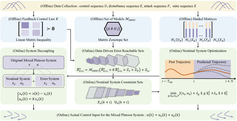
Figure 2: Schematic of the proposed RDeeP-LCC method for mixed platoons. In the offline learning phase (blue), the method utilizes pre-collected data (yellow) to calculate the over-approximated system matrix set $\mathcal{M}_{ABHJ}$, derive a data-driven feedback control law $K$ to ensure stability for all possible systems, and generate the Hankel matrices. In the online control phase (green), the RDeeP-LCC solves for optimal control input for the CAV in a receding horizon strategy. Specifically, The system is decomposed into the error system and the nominal system. Using $\mathcal{M}_{ABHJ}$ and $K$, the method recursively derives the data-driven reachable set of error states, and then subtracts this set from the constraints of the original system to obtain a more compact nominal system constraint. Then, the nominal control input $u_{\mathrm{z}}(k)$ is calculated using the standard DeeP-LCC under the compact nominal constraint. Finally, the actual control input of the CAV is obtained by combining the nominal control input $u_{\mathrm{z}}(k)$ with the error feedback control input $u_{\mathrm{e}}(k)$ in a tube-based control manner.

III-A Data Collection

In this study, we collect offline data by exciting the mixed platoon system by applying small control inputs to the CAV, attack inputs to the CAV, and disturbances to the head vehicle, respectively. From the parametric model of the mixed platoon system (9), it can be found that the state $x(k)$ is affected by the control input $u(k)$, head vehicle’s velocity deviation ${\epsilon}(k)$, the adversarial attacks $\vartheta(k)$, and the process noise $\omega(k)$. Note that during data collection, $u(k),{\epsilon}(k),\vartheta(k),x(k)$ are all measurable, while $\omega(k)$ is unknown but bounded. This paper applies a sequence of persistently exciting inputs $u(k)$, $\epsilon(k)$, and $\vartheta(k)$ with a length $T+1$ to the mixed platoon system for data collection. Specifically, the control input sequence $U$, the disturbance input sequence $E$, the adversarial attack sequence $F$, and the corresponding state sequence $X$ are defined as follows:

$$U=[u(1),u(2),\ldots,u(T+1)]\in\mathbb{R}^{1\times(T+1)},$$ (14a)

$$E=[\epsilon(1),\epsilon(2),\ldots,\epsilon(T+1)]\in\mathbb{R}^{1\times(T+1)},$$ (14b)

$$F=[\vartheta(1),\vartheta(2),\ldots,\vartheta(T+1)]\in\mathbb{R}^{1\times(T+1)},$$ (14c)

$$X=[x(1),x(2),\ldots,x(T+1)]\in\mathbb{R}^{2n\times(T+1)}.$$ (14d)

These data are all measurable, and will be processed into standardized formats to construct matrix zonotope set $\mathcal{M}_{ABHJ}$ for reachable set computation and Hankel matrices for future trajectory predictions, respectively, as shown in Figure 2. Particularly, for constructing matrix zonotope set $\mathcal{M}_{ABHJ}$, the data sequences are further reorganized as:

$$U_{-}=[u(1),u(2),\ldots,u(T)]\in\mathbb{R}^{1\times T},$$ (15a)

$$E_{-}=[\epsilon(1),\epsilon(2),\ldots,\epsilon(T)]\in\mathbb{R}^{1\times T},$$ (15b)

$$F_{-}=[\vartheta(1),\vartheta(2),\ldots,\vartheta(T)]\in\mathbb{R}^{1\times T},$$ (15c)

$$X_{-}=[x(1),x(2),\ldots,x(T)]\in\mathbb{R}^{2n\times T},$$ (15d)

$$X_{+}=[x(2),x(3),\ldots,x(T+1)]\in\mathbb{R}^{2n\times T}.$$ (15e)

In addition, for convenience in the subsequent derivations, the sequence of unknown noise is denoted as

$$W_{-}=[\omega(1),\omega(2),\ldots,\omega(T)]\in\mathbb{R}^{2n\times T},$$ (16)

although it is important to note that $W_{-}$ is not directly measurable.

For constructing Hankel matrices in future trajectory predictions, we reformulate the trajectory data $U_{-}$, $E_{-}$, $F_{-}$, and $X_{-}$ into a compact form as the following column vectors:

$$U_{\mathrm{d}}={\mathrm{col}}(U_{-})\in\mathbb{R}^{T},$$ (17a)

$$E_{\mathrm{d}}={\mathrm{col}}(E_{-})\in\mathbb{R}^{T},$$ (17b)

$$F_{\mathrm{d}}={\mathrm{col}}(F_{-})\in\mathbb{R}^{T},$$ (17c)

$$X_{\mathrm{d}}={\mathrm{col}}(X_{-})\in\mathbb{R}^{2nT}.$$ (17d)

III-B Offline Learning

In the offline learning phase, given that the matrices $A$, $B$, $H$, and $J$ in (9) are unknown, we utilize pre-collected data to construct an over-approximated system matrix set $\mathcal{M}_{ABHJ}$. This set models the unknown and uncertain dynamics of the mixed platoon system. We then derive a data-driven stabilizing feedback control law $K$ from data to ensure stability across all possible systems configurations represented by $\begin{bmatrix}A~{}B\end{bmatrix}$. Additionally, the Hankel matrices, defined in Definition 5, are formed using the pre-collected data and serve as part of the predictor. These components, the over-approximated system matrix set $\mathcal{M}_{ABHJ}$, the stabilizing feedback control law $K$, and the Hankel matrices, are later integral to the online control phase, discussed in Section III-C.

III-B1 Over-Approximated System Matrix Set

We first construct the matrix zonotope set $\mathcal{M}_{ABHJ}$ to over-approximate all possible system models $\begin{bmatrix}A~{}B~{}H~{}J\end{bmatrix}$ that are consistent with the noisy data. The following Lemma 2 is needed.

Lemma 2

Given the data sequences $U_{-}$, $E_{-}$, $F_{-}$, $X_{-}$, and $X_{+}$ from the mixed platoon system (9). And transforming the bounded forms of the disturbance $\epsilon(k)$, the attack $\vartheta(k)$, and the noise $\omega(k)$ in (10) to be zonotope sets, given by:

$$\epsilon(k)\in\mathcal{Z}_{\epsilon},\quad\vartheta(k)\in\mathcal{Z}_{\vartheta},\quad\omega(k)\in\mathcal{Z}_{\omega}.$$ (18)

If the matrix $\begin{bmatrix}X_{-}^{\top}~{}U_{-}^{\top}~{}E_{-}^{\top}~{}F_{-}^{\top}\end{bmatrix}^{\top}$ is of full row rank, then the set of all possible $\begin{bmatrix}A~{}B~{}H~{}J\end{bmatrix}$ can be obtained:

$$\mathcal{M}_{ABHJ}=\left(X_{+}-\mathcal{M}_{\omega}\right)\begin{bmatrix}X_{-}\\ U_{-}\\ E_{-}\\ F_{-}\end{bmatrix}^{\dagger},$$ (19)

where $\dagger$ is the Moore–Penrose pseudoinverse of the matrix, and we have the noise set given by

$$\mathcal{M}_{\omega}=\left\langle C_{\mathcal{M}_{\omega}},\left[G_{\mathcal{M}_{\omega}}^{(1)},G_{\mathcal{M}_{\omega}}^{(2)},\ldots,G_{\mathcal{M}_{\omega}}^{(\gamma_{\mathcal{M}_{\omega}})}\right]\right\rangle,$$ (20)

which is a matrix zonotope set resulting from the noise zonotope $\mathcal{Z}_{\omega}=\left\langle c_{\mathcal{Z}_{\omega}},G_{\mathcal{Z}_{\omega}}\right\rangle$, with $G_{\mathcal{Z}_{\omega}}=\left[g_{\mathcal{Z}_{\omega}}^{(1)},g_{\mathcal{Z}_{\omega}}^{(2)},\cdots,g_{\mathcal{Z}_{\omega}}^{(\gamma_{\mathcal{Z}_{\omega}})}\right]$, where $\gamma_{\mathcal{M}_{\omega}}\in\mathbb{N}$ is the number of generator matrices. Specific formulations in (20) are given as follows:

$$C_{\mathcal{M}_{\omega}}=\begin{bmatrix}c_{\mathcal{Z}_{\omega}}&\ldots&c_{\mathcal{Z}_{\omega}}\end{bmatrix},$$ (21a)

$$G_{\mathcal{M}_{\omega}}^{(1+(i-1)T)}=\begin{bmatrix}g_{\mathcal{Z}_{\omega}}^{(i)}&0_{n\times(T-1)}\end{bmatrix},$$ (21b)

$$G_{\mathcal{M}_{\omega}}^{(j+(i-1)T)}=\begin{bmatrix}0_{n\times(j-1)}&g_{\mathcal{Z}_{\omega}}^{(i)}&0_{n\times(T-j)}\end{bmatrix},$$ (21c)

$$G_{\mathcal{M}_{\omega}}^{(T+(i-1)T)}=\begin{bmatrix}0_{n\times(T-1)}&g_{\mathcal{Z}_{\omega}}^{(i)}\end{bmatrix},$$ (21d)

with $\forall i=\left\{1,2,\cdots,\gamma_{\mathcal{Z}_{w}}\right\}$ and $j=\{2,3,\cdots,T-1\}$.

Proof: For the system description in (9), we have

$$X_{+}=\begin{bmatrix}A~{}B~{}H~{}J\end{bmatrix}\begin{bmatrix}X_{-}\\ U_{-}\\ E_{-}\\ F_{-}\end{bmatrix}+W_{-}.$$ (22)

Since the matrix $\begin{bmatrix}X_{-}^{\top}~{}U_{-}^{\top}~{}E_{-}^{\top}~{}F_{-}^{\top}\end{bmatrix}^{\top}$ is of full row rank, then we could get

$$\begin{bmatrix}A~{}B~{}H~{}J\end{bmatrix}=\left(X_{+}-W_{-}\right)\begin{bmatrix}X_{-}\\ U_{-}\\ E_{-}\\ F_{-}\end{bmatrix}^{\dagger},$$ (23)

where the noise $W_{-}$ in the collected data is unknown, but one can use the corresponding bounds $\mathcal{M}_{\omega}$ to obtain (19). Then, the matrix zonotope set $\mathcal{M}_{ABHJ}$ is an over-approximation for system models $\begin{bmatrix}A~{}B~{}H~{}J\end{bmatrix}$ considering noisy data. $\hfill\blacksquare$

III-B2 Data-Driven Stabilizing Feedback Control Law

We then aim to stabilize all possible $\begin{bmatrix}A~{}B\end{bmatrix}$ by a feedback law $K$. Collect data under the condition that $\epsilon(k)=0$ and $\vartheta(k)=0$, which are straightforward to achieve. Inspired by [52], we assume the data sequence $W_{-}$ satisfies a quadratic matrix inequality:

$$\begin{bmatrix}I\\ W_{-}\end{bmatrix}^{\top}\Phi\begin{bmatrix}I\\ W_{-}\end{bmatrix}\geq 0,$$ (24)

where $\Phi=\begin{bmatrix}\Phi_{11}~{}\Phi_{12}\\ \Phi_{21}~{}\Phi_{22}\end{bmatrix}\in\mathbb{S}^{2n+T}$, with $\Phi_{11}\in\mathbb{S}^{2n}$, $\Phi_{12}\in\mathbb{R}^{2n\times T}$, $\Phi_{21}\in\mathbb{R}^{T\times 2n}$, $\Phi_{22}\in\mathbb{S}^{T}$. Based on the bound of $\omega(k)$ in $W_{-}$ as described in (10), where $\left\|\omega(k)\right\|_{\infty}\leq\omega_{\mathrm{max}}$, we set $\Phi_{22}=-I$, $\Phi_{12}=0$, and $\Phi_{11}=\omega_{\mathrm{max}}^{2}TI$.

Then, the feedback control law $K$ that stabilizes all possible systems $\begin{bmatrix}A~{}B\end{bmatrix}$ can be obtained by Lemma 3.

Lemma 3

For mixed platoon systems (9), if the assumption in (24) hold and the matrix $\begin{bmatrix}X_{-}^{\top}~{}U_{-}^{\top}\end{bmatrix}^{\top}$ is of full row rank, one can solve the following linear matrix inequalities (LMIs):

$$\begin{bmatrix}P&0\\ 0&-P\end{bmatrix}-\begin{bmatrix}I&X_{+}\\ 0&-X_{-}\end{bmatrix}\Phi\begin{bmatrix}I&X_{+}\\ 0&-X_{-}\end{bmatrix}^{\top}>0,$$ (25a)

$$P-\begin{bmatrix}I&X_{+}\end{bmatrix}\Phi\begin{bmatrix}I\\ X_{+}^{\top}\end{bmatrix}+\Theta\begin{bmatrix}X_{-}\\ U_{-}\end{bmatrix}^{\top}\Psi\begin{bmatrix}X_{-}\\ U_{-}\end{bmatrix}\Theta^{\top}>0,$$ (25b)

$$\Psi=\left(\begin{bmatrix}X_{-}\\ U_{-}\end{bmatrix}\Phi_{22}\begin{bmatrix}X_{-}\\ U_{-}\end{bmatrix}^{\top}\right)^{-1},$$ (25c)

to obtain the positive definite matrix $P$, where $\Theta=\Phi_{12}+X_{+}\Phi_{22}$. Using $P$, the feedback gain can be obtained by

$$K=\left(U_{-}\left(\Phi_{22}+\Theta^{\top}\Gamma^{\dagger}\Theta\right)X_{-}^{\top}\right)\left(X_{-}\left(\Phi_{22}+\Theta^{\top}\Gamma^{\dagger}\Theta\right)X_{-}^{\top}\right)^{\dagger},$$ (26)

which stabilizes all possible systems $\begin{bmatrix}A~{}B\end{bmatrix}$, where

$$\Gamma=P-\begin{bmatrix}I&X_{+}\end{bmatrix}\Phi\begin{bmatrix}I\\ X_{+}^{\top}\end{bmatrix}.$$ (27)

Proof: Lemma 3 is derived from [52, Theorem 5.3], with a detailed proof available in [52].$\hfill\blacksquare$

III-B3 Hankel Matrices

We finally utilize the pre-collected data $U_{d}$, $E_{d}$, $F_{d}$, $X_{d}$ to form the Hankel matrices by Definition 5, which constitute part of the data-driven model used during online control in Section III-B. In particular, these matrices are partitioned into two parts, corresponding to the trajectory data in the past $T_{\mathrm{ini}}\in\mathbb{N}$ steps and the trajectory data in the future $N\in\mathbb{N}$ steps, defined as follows:

$$\begin{split}&\begin{bmatrix}U_{\mathrm{p}}\\ U_{\mathrm{f}}\end{bmatrix}=\mathcal{H}_{L}(U_{\mathrm{d}}),\begin{bmatrix}E_{\mathrm{p}}\\ E_{\mathrm{f}}\end{bmatrix}=\mathcal{H}_{L}(E_{\mathrm{d}}),\\ &\begin{bmatrix}F_{\mathrm{p}}\\ F_{\mathrm{f}}\end{bmatrix}=\mathcal{H}_{L}(F_{\mathrm{d}}),\begin{bmatrix}X_{\mathrm{p}}\\ X_{\mathrm{f}}\end{bmatrix}=\mathcal{H}_{L}(X_{\mathrm{d}}),\end{split}$$ (28)

where $L=T_{\mathrm{ini}}+N$, and $U_{\mathrm{p}},U_{\mathrm{f}}$ contain the upper $T_{\mathrm{ini}}$ rows and lower $N$ rows of $\mathcal{H}_{L}(U_{\mathrm{d}})$, respectively (similarly for $E_{\mathrm{p}}$ and $E_{\mathrm{f}}$, $F_{\mathrm{p}}$ and $F_{\mathrm{f}}$, $X_{\mathrm{p}}$ and $X_{\mathrm{f}}$).

Remark 2

Note that for the persistently exciting requirement of order $T_{\mathrm{ini}}+N$, one sufficient condition is $T\geq 2\left(T_{\mathrm{ini}}+N+2n\right)-1$ [34, 37]. This ensures that the input sequences $U_{-}$, $E_{-}$, and $F_{-}$ are sufficiently long to excite the system fully. The generated state sequence $X_{-}$ could capture the dynamic behavior of the mixed platoon under the influence of multi-source inputs.

III-C Online Control

To ensure the robustness of the mixed platoon control system under process noise and adversarial attacks, the reachable set technique is introduced. Inspired by the tube-based control method [53] and reach-avoid control method [54], the system is first decoupled into a nominal system and an error system. The reachable set of the error system is computed under disturbances, attacks, and noise. Then, the reachable set of the nominal system is obtained by subtracting the error reachable set from the practical constraints. Using these compact nominal constraints, the nominal control input is computed via the standard DeeP-LCC. Finally, the actual control input for the CAV is obtained by combining the nominal control input with the error feedback control input.

III-C1 Mixed Platoon System Decoupling

We start by employing the parametric system model (9) to illustrate the decoupling process. The decoupled nominal system and the error system are denoted as follows:

$${x}_{\mathrm{z}}(k+1)=A{x}_{\mathrm{z}}(k)+B{u}_{\mathrm{z}}(k)+H\epsilon_{\mathrm{z}}(k)+J\vartheta_{\mathrm{z}}(k),$$ (29a)

$${x}_{\mathrm{e}}(k+1)=A{x}_{\mathrm{e}}(k)+Bu_{\mathrm{e}}(k)+H\epsilon_{\mathrm{e}}(k)+J\vartheta_{\mathrm{e}}(k)+\omega(k),$$ (29b)

where ${x}_{\mathrm{z}}(k)$, $u_{\mathrm{z}}(k)$, $\epsilon_{\mathrm{z}}(k)$, $\vartheta_{\mathrm{z}}(k)$ and ${x}_{\mathrm{e}}(k)$, $u_{\mathrm{e}}(k)$, $\epsilon_{\mathrm{e}}(k)$, $\vartheta_{\mathrm{e}}(k)$ represent the state, control input, disturbance input, and attack input of the nominal dynamics system and error dynamics system, respectively. Specifically, we have

$$\begin{cases}{x}(k)={x}_{\mathrm{z}}(k)+{x}_{\mathrm{e}}(k),\\ {u}(k)={u}_{\mathrm{z}}(k)+{u}_{\mathrm{e}}(k),\\ {\epsilon}(k)={\epsilon}_{\mathrm{z}}(k)+{\epsilon}_{\mathrm{e}}(k),\\ {\vartheta}(k)={\vartheta}_{\mathrm{z}}(k)+{\vartheta}_{\mathrm{e}}(k).\\ \end{cases}$$ (30)

Particularly, we set

$${\epsilon}_{\mathrm{z}}(k)=0,\quad{\epsilon}_{\mathrm{e}}(k)={\epsilon}(k),\quad{\vartheta}_{\mathrm{z}}(k)=0,\quad{\vartheta}_{\mathrm{e}}(k)={\vartheta}(k),$$ (31)

so that the disturbance $\epsilon(k)$, the attack $\vartheta(k)$, and the noise $\omega(k)$ are considered exclusively in the error system, without affecting the nominal system. This simplifies the solution of the RDeeP-LCC optimization formulation in the following.

III-C2 Data-Driven Reachable Set of Error State

Based on the process noise, disturbance, and attack zonotope sets defined in (18), the model matrix zonotope set $\mathcal{M}_{ABHJ}$ derived in (19), and linear state feedback gain $K$ derived in (26), we can compute the error state reachable set using Lemma 4 for the error dynamics described in (29b).

Lemma 4

For the system described by (29b), given input-state trajectories $U_{-}$, $E_{-}$, $F_{-}$, $X_{-}$, $X_{+}$, if the matrix $\begin{bmatrix}X_{-}^{\top}~{}U_{-}^{\top}~{}E_{-}^{\top}~{}F_{-}^{\top}\end{bmatrix}^{\top}$ is of full row rank, then the recursive relation for the data-driven error state reachable set can be computed as follows:

$$\hat{\mathcal{R}}^{\mathrm{e}}_{k+i+1}=\mathcal{M}_{ABHJ}\left(\hat{\mathcal{R}}^{\mathrm{e}}_{k+i}\times K\hat{\mathcal{R}}^{\mathrm{e}}_{k+i}\times\mathcal{Z}_{\epsilon}\times\mathcal{Z}_{\vartheta}\right)+\mathcal{Z}_{\omega},$$ (32)

where $\hat{\mathcal{R}}^{\mathrm{e}}_{k+i}$ represents an over-approximated reachable set for the state $x_{\mathrm{e}}(k+i)$ of the error dynamics system (29b).

Proof: From the error dynamics system (29b), the error state reachable set can be computed using the model:

$$\mathcal{R}_{k+i+1}^{\mathrm{e}}=\begin{bmatrix}A~{}B~{}H~{}J\end{bmatrix}\left(\mathcal{R}_{k+i}^{\mathrm{e}}\times K{\mathcal{R}}_{k+i}^{\mathrm{e}}\times\mathcal{Z}_{\epsilon}\times\mathcal{Z}_{\vartheta}\right)+\mathcal{Z}_{\omega}.$$ (33)

Since $\begin{bmatrix}A~{}B~{}H~{}J\end{bmatrix}\in\mathcal{M}_{ABHJ}$, according to Lemma 2, and if $\mathcal{R}_{k+i}^{\mathrm{e}}$ and $\hat{\mathcal{R}}_{k+i}^{\mathrm{e}}$ start from the same initial set, it is evident that ${\mathcal{R}}_{k+i+1}^{\mathrm{e}}\in\hat{\mathcal{R}}_{k+i+1}^{\mathrm{e}}$. Therefore, the recursive relation (32) holds, providing an over-approximated reachable set for the data-driven error state. $\hfill\blacksquare$

III-C3 RDeeP-LCC Optimization Formulation

In this part, we proceed to design the RDeeP-LCC optimization formulation, which is extended from DeeP-LCC [34], for the mixed platoon to achieve optimal and safe control under external disturbance ${\epsilon}(k)$, adversarial attacks ${\vartheta}(k)$, and process noise $\omega(k)$.

a) Trajectory Definition: At each time step $k$, we define the state trajectory $x_{\mathrm{ini}}$ over the past $T_{\mathrm{ini}}$ steps and the future state trajectory $x_{z}$ of the nominal system in the next $N$ steps as follows:

$$\begin{cases}x_{\mathrm{ini}}&=\mathrm{col}(x(k-T_{\mathrm{ini}}),x(k-T_{\mathrm{ini}}+1),\ldots,x(k-1)),\\ x_{\mathrm{z}}&=\mathrm{col}(x_{\mathrm{z}}(k),x_{\mathrm{z}}(k+1),\ldots,x_{\mathrm{z}}(k+N-1)).\end{cases}$$ (34)

The control input trajectories $u_{\mathrm{ini}}$ and $u_{\mathrm{z}}$, the disturbance input trajectories $\epsilon_{\mathrm{ini}}$ and $\epsilon_{\mathrm{z}}$, and the attack input trajectories $\vartheta_{\mathrm{ini}}$ and $\vartheta_{\mathrm{z}}$ in the past $T_{\mathrm{ini}}$ steps and future $N$ steps are defined similarly as in (34).

b) Cost Function: Similarly to DeeP-LCC [34], we utilize the quadratic function $J(x_{\mathrm{z}},u_{\mathrm{z}})$ to quantify the control performance by penalizing the states $x_{\mathrm{z}}$ and control inputs $u_{\mathrm{z}}$ of the nominal system (29a), defined as follows:

$$J(x_{\mathrm{z}},u_{\mathrm{z}})=\sum_{i=0}^{N-1}\left(\|x_{\mathrm{z}}(k+i)\|_{Q}^{2}+\|u_{\mathrm{z}}(k+i)\|_{R}^{2}\right),$$ (35)

where $Q=\operatorname{diag}\left(Q_{x},\xi Q_{x},\ldots,\xi^{(n-1)}Q_{x}\right)\in\mathbb{R}^{2n\times 2n}$ and $R\in\mathbb{R}$ are the weight matrices penalizing the system states and control inputs, with $0<\xi\leq 1$ denotes the decay factor. By this design, we will put less penalty for those HDVs far from the CAV. Precisely, we have $Q_{x}=\operatorname{diag}\left(\rho_{s},\rho_{v}\right)$, with $\rho_{s}$ and $\rho_{v}$ denoting the penalty weights for spacing deviation and velocity deviation, respectively.

c) Data-Driven Dynamics: Based on Willems’ Fundamental Lemma (Lemma 1) and [34, Proposition 2], the data-driven dynamics of the mixed platoon system can be given by

$$\begin{bmatrix}X_{\mathrm{p}}\\ U_{\mathrm{p}}\\ E_{\mathrm{p}}\\ F_{\mathrm{p}}\\ X_{\mathrm{f}}\\ U_{\mathrm{f}}\\ E_{\mathrm{f}}\\ F_{\mathrm{f}}\end{bmatrix}g=\begin{bmatrix}x_{\mathrm{ini}}\\ u_{\mathrm{ini}}\\ \epsilon_{\mathrm{ini}}\\ \vartheta_{\mathrm{ini}}\\ x_{\mathrm{z}}\\ u_{\mathrm{z}}\\ \epsilon_{\mathrm{z}}\\ \vartheta_{\mathrm{z}}\end{bmatrix}.$$ (36)

The existence of $g\in\mathbb{R}^{T-T_{\mathrm{ini}}-N+1}$ satisfying (36) implies that $x_{\mathrm{z}}$, $u_{\mathrm{z}}$, $\epsilon_{\mathrm{z}}$, and $\vartheta_{\mathrm{z}}$ form a future trajectory of length $N$. Note that to ensure the uniqueness of the future trajectory $x_{\mathrm{z}}$ for given $x_{\mathrm{ini}}$, $u_{\mathrm{ini}}$, $\epsilon_{\mathrm{ini}}$, $\vartheta_{\mathrm{ini}}$, $u_{\mathrm{z}}$, $\epsilon_{\mathrm{z}}$, $\vartheta_{\mathrm{z}}$, it is required that $T_{\mathrm{ini}}\geq 2n$ [55].

Remark 3

The data-driven dynamics (36) allows one to bypass system identification and directly predict the future trajectory of the nominal system (29a) using a non-parametric approach. Specifically, the state trajectory $x_{\mathrm{z}}$ can be directly obtained once $u_{\mathrm{z}}$, ${\epsilon}_{\mathrm{z}}$, and ${\vartheta}_{\mathrm{z}}$ are determined. Furthermore, recall that the data Hankel matrices $X_{\mathrm{p}}$, $U_{\mathrm{p}}$, $E_{\mathrm{p}}$, $F_{\mathrm{p}}$, $X_{\mathrm{f}}$, $U_{\mathrm{f}}$, $E_{\mathrm{f}}$, and $F_{\mathrm{f}}$ in (36) are calculated offline using (28) with pre-collected data.

d) Constraints: The safety of the mixed platoon system is ensured by imposing the following constraints:

$$\begin{cases}x(k+i)\in\mathcal{X},\\ u(k+i)\in\mathcal{U},\end{cases}$$ (37)

where $\mathcal{X}=\left\{x(k)\in\mathbb{R}^{2n}\mid|x(k)|\leq\mathbf{1}_{n}\otimes x_{\max}\right\}$ is the state constraint, with $x_{\max}=\left[\tilde{s}_{\max},\tilde{v}_{\max}\right]^{\top}$, where $\tilde{s}_{\max}$ and $\tilde{v}_{\max}$ are the constraint limits for spacing deviation and velocity deviation, respectively. For the control input constraint, we define $\mathcal{U}=\left\{u(k)\in\mathbb{R}\mid|u(k)|\leq u_{\max}\right\}$, where $u_{\max}$ denotes the maximum control input for the CAVs.

Combining (32) and (37), the constraint set for the nominal system (29a) can be calculated as follows:

$$\begin{cases}\mathcal{X}_{\mathrm{z}}(k+i)=\mathcal{X}-\hat{\mathcal{R}}_{k+i}^{\mathrm{e}},\\ \mathcal{U}_{\mathrm{z}}(k+i)=\mathcal{U}-K\hat{\mathcal{R}}_{k+i}^{\mathrm{e}},\end{cases}$$ (38)

which yields the constraints for the predicted trajectory of the nominal system (29a), given by:

$$\begin{cases}x_{\mathrm{z}}(k+i)\in\mathcal{X}_{\mathrm{z}}(k+i),\\ u_{\mathrm{z}}(k+i)\in\mathcal{U}_{\mathrm{z}}(k+i).\end{cases}$$ (39)

For the future disturbance sequence $\epsilon_{\mathrm{z}}$ and attack sequence $\vartheta_{\mathrm{z}}$ of the nominal system, recalling (31), we have

$$\epsilon_{\mathrm{z}}(k+i)=0,\quad\vartheta_{\mathrm{z}}(k+i)=0.$$ (40)

e) RDeeP-LCC Optimization Problem: Naturally, we could formulate the optimization problem to solve the control input for the CAVs in mixed platoon systems as follows:

$$\min\limits_{g,u_{\mathrm{z}},x_{\mathrm{z}}} J(x_{\mathrm{z}},u_{\mathrm{z}})$$ (41)

$$\mathrm{s.t.} \eqref{Eq:WilliemExpanding},~{}\eqref{Eq:NormalConstraint},~{}\eqref{Eq:DisturbanceConstraint}.$$

Solving this optimization problem (41) could yield the optimal sequence of future control inputs $u_{\mathrm{z}}$ and the corresponding sequence of state outputs $x_{\mathrm{z}}$ of the mixed platoon system. However, the data-centric dynamics model (36) could provide no feasible solutions due to the uncertainty, nonlinear factor, and process noise. Motivated by the literature [36, 34], we ensure the feasibility of the optimization problem (41) by introducing a slack variable $\sigma\in\mathbb{R}^{2nT_{\mathrm{ini}}}$ in (36) as follows:

$$\begin{bmatrix}X_{\mathrm{p}}\\ U_{\mathrm{p}}\\ E_{\mathrm{p}}\\ F_{\mathrm{p}}\\ X_{\mathrm{f}}\\ U_{\mathrm{f}}\\ E_{\mathrm{f}}\\ F_{\mathrm{f}}\end{bmatrix}g=\begin{bmatrix}x_{\mathrm{ini}}\\ u_{\mathrm{ini}}\\ \epsilon_{\mathrm{ini}}\\ \vartheta_{\mathrm{ini}}\\ x_{\mathrm{z}}\\ u_{\mathrm{z}}\\ \epsilon_{\mathrm{z}}\\ \vartheta_{\mathrm{z}}\end{bmatrix}+\begin{bmatrix}\sigma\\ 0\\ 0\\ 0\\ 0\\ 0\\ 0\\ 0\end{bmatrix},$$ (42)

and penalizing $g$ with regularization. The final RDeeP-LCC optimization problem for mixed platoon control is constructed as

$$\min\limits_{g,u_{\mathrm{z}},x_{\mathrm{z}},\sigma} J(x_{\mathrm{z}},u_{\mathrm{z}})+\lambda_{g}\|g\|_{2}^{2}+\lambda_{\sigma}\|\sigma\|_{2}^{2}$$ (43)

$$\mathrm{s.t.} \eqref{Eq:NormalConstraint},~{}\eqref{Eq:DisturbanceConstraint},~{}\eqref{Eq:WilliemExpandingSlack},$$

where $\lambda_{g}$ and $\lambda_{\sigma}$ denote the regularization penalty coefficients for the weighted two-norm for $g$ and $\sigma$, respectively. Intuitively, $\lambda_{g}\geq 0$ reduces the overfitting risk of data-driven dynamics, and $\lambda_{\sigma}\geq 0$ ensures the feasibility of the optimization problem solution.

Solving (43) yields an optimal control sequence $u_{\mathrm{z}}$ and the predicted state sequence $x_{\mathrm{z}}$ of the nominal system. Then, by

$$u(k)=u_{\mathrm{z}}(k)+K({x}(k)-{x}_{\mathrm{z}}(k)),$$ (44)

we obtain the final control input for the CAV, where ${x}(k)$ is measured from the actual system, and $K$ is offline calculated from (26).

For each time step $k$ of the online data-driven predictive control, we solve the final RDeeP-LCC optimization problem (43) using the receding horizon technique. The detailed procedure of RDeeP-LCC is presented in Algorithm 1.

Input: Pre-collected data ($U$, $E$, $F$, $X$), constraints ($\mathcal{X}$, $\mathcal{U}$), weight ($Q$, $R$), bounded $\mathcal{Z}_{{\epsilon}}$, $\mathcal{Z}_{\vartheta}$, and $\mathcal{Z}_{\omega}$, past horizon $T_{\mathrm{ini}}$, control horizon $N$, total number of steps $N_{f}$.

1

2Construct data ($U_{-}$, $E_{-}$, $F_{-}$, $X_{-}$, $X_{+}$) and data ($U_{\mathrm{d}}$, $E_{\mathrm{d}}$, $F_{\mathrm{d}}$, $X_{\mathrm{d}}$);

3 Offline construct data Hankel matrices $U_{\mathrm{p}}$, $U_{\mathrm{f}}$, $E_{\mathrm{p}}$, $E_{\mathrm{f}}$, $F_{\mathrm{p}}$, $F_{\mathrm{f}}$, $X_{\mathrm{p}}$, $X_{\mathrm{f}}$ using (28), the matrix zonotope set $\mathcal{M}_{ABHJ}$ using (19), and the feedback control law $K$ using (32) ;

4 Initialize past mixed platoon data ($x_{\mathrm{ini}}$, $u_{\mathrm{ini}}$, ${\epsilon}_{\mathrm{ini}}$, ${\vartheta}_{\mathrm{ini}}$) at the initial time step $0$;

5

6while $0\leq k\leq N_{f}$ do

7       Compute data-driven error reachable sets to obtain $\hat{\mathcal{R}}_{k+i}^{\mathrm{e}}$ using (32);

8       Compute constraint set for the nominal system to obtain $\mathcal{X}_{\mathrm{z}}(k+i)$ and $\mathcal{U}_{\mathrm{z}}(k+i)$ using (38);

9       Solve (43) to obtain the optimal control input sequence and the state sequence for the nominal system $u_{\mathrm{z}}=\mathrm{col}(u_{\mathrm{z}}(k),u_{\mathrm{z}}(k+1),\cdots,u_{\mathrm{z}}(k+N-1))$ $x_{\mathrm{z}}=\mathrm{col}(x_{\mathrm{z}}(k),x_{\mathrm{z}}(k+1),\cdots,x_{\mathrm{z}}(k+N-1))$;

10      

11      Measure the actual state $x(k)$ from the actual system;

12      

13      Obtain $u(k)$ from (44) and apply it as the control input to the CAV;

14       $k\leftarrow k+1$ and update past mixed platoon data ($x_{\mathrm{ini}}$, $u_{\mathrm{ini}}$, ${\epsilon}_{\mathrm{ini}}$, ${\vartheta}_{\mathrm{ini}}$);

15      

16 end while

Algorithm 1 RDeeP-LCC

Remark 4

It is worth noting that in (43), $x_{\mathrm{ini}},u_{\mathrm{ini}},\epsilon_{\mathrm{ini}},\vartheta_{\mathrm{ini}}$ represent the past trajectories of the actual system (9), while $x_{z},u_{\mathrm{z}},\epsilon_{\mathrm{z}},\vartheta_{\mathrm{z}}$ denote the predicted trajectories of the nominal system (29a). As shown in (31), we assume $\epsilon_{\mathrm{z}}(k)=0$ and $\vartheta_{\mathrm{z}}(k)=0$, and capture the actual disturbances $\epsilon_{\mathrm{e}}(k)=\epsilon(k)$ and actual attacks $\vartheta_{\mathrm{e}}(k)=\vartheta(k)$ solely in the error system (29b). Provided $\epsilon(k)\in\mathcal{Z}_{\epsilon}$ and $\vartheta(k)\in\mathcal{Z}_{\vartheta}$ in (18), the effects of disturbances and attacks are further incorporated into the calculation of the error reachable set (32), resulting in a more stringent constraint (39) on $x_{\mathrm{z}}$ and $u_{\mathrm{z}}$ of the nominal system. This approach addresses the influence of unknown future disturbances and attacks, which are often oversimplified as zero in previous research [34, 40, 39].

IV Numerical Simulation

In this section, we conduct numerical simulations to evaluate the effectiveness of the proposed RDeeP-LCC method for mixed platoons in the presence of noise and attacks.

IV-A Simulation Setup

For the simulations, we consider the mixed platoon configuration depicted in Figure1, setting the platoon size to $n=3$. We model the dynamics of CAVs using (5), while the specific dynamics of HDVs in (2) are captured by the nonlinear OVM model [22], given by:

$$u_{i}(t)=\alpha_{i}\left(V\left(s_{i}(t)\right)-v_{i}\right)+\beta_{i}\left(v_{i-1}(t)-v_{i}(t)\right),\quad i\in\Omega_{\mathrm{H}}$$ (45)

where $\alpha_{i}$ and $\beta_{i}$ denote the driver’s sensitivity parameters to the deviation between desired and actual velocities, and the velocity deviation between the vehicle $i$ and its preceding vehicle $i-1$, respectively. The desired velocity $V\left(s_{i}(t)\right)$ is defined as follows:

$$V\left(s_{i}(t)\right)=\begin{cases}0,&s_{i}(t)\leq s_{\min}\\ f_{v}\left(s_{i}(t)\right),&s_{\min}<s_{i}(t)<s_{\max}\\ v_{\max},&s_{i}(t)\geq s_{\max},\end{cases}\quad i\in\Omega_{\mathrm{H}}$$ (46)

where $v_{\max}$ is the maximum velocity, and $s_{\max}$ and $s_{\min}$ denote the maximum and minimum spacing, respectively. Referencing [11], the nonlinear expression for $f_{v}\left(s_{i}(t)\right)$ is given as follows:

$$f_{v}\left(s_{i}(t)\right)=\frac{v_{\max}}{2}\left(1-\cos\left(\pi\frac{s_{i}(t)-s_{\min}}{s_{\max}-s_{\min}}\right)\right).\quad i\in\Omega_{\mathrm{H}}$$ (47)

It is important to note that these models are solely used for state updates of the vehicles in the simulations, and are not integrated into the proposed data-driven control scheme. The parameters for HDVs are set as $\alpha_{i}=0.6$, $\beta_{i}=0.9$, $v_{\max}=36$, $s_{\max}=35$, and $s_{\min}=5$ in (45)-(47). The simulation parameters for the RDeeP-LCC are specified as follows:

• For data collection phase, around the equilibrium velocity of $v^{*}=$18\text{\,}\mathrm{m}\mathrm{/}\mathrm{s}$$, we generate random control inputs of the CAV by $u(t)\sim\mathbb{U}\left[-0.2,0.2\right]$, random disturbance inputs for the head vehicle’s velocity by $\epsilon(t)\sim\mathbb{U}\left[-0.5,0.5\right]$, and random attack inputs by $\vartheta(t)\sim\mathbb{U}\left[-0.3,0.3\right]$, where $\mathbb{U}$ represents uniform distribution. The offline pre-collected trajectories, with a length of $T=600$ and a sampling interval of $0.05\text{\,}\mathrm{s}$, are then employed to construct (14)-(17).

• For offline learning phase, based on these pre-collected data sequences, we derive the over-approximated system matrix set $\mathcal{M}_{ABHJ}$ using (19), compute the feedback control law $K$ using (26) in Lemma 3, and construct the Hankel matrices using (28), satisfying the persistently exciting condition as discussed in [34, 37].

• For online control phase, the future sequence length is set to $N=5$ and the past sequence length is chosen as $T_{\mathrm{ini}}=20$ for the state trajectory (34). The cost function (35) is configured with weight coefficients $\xi=0.6$, $\rho_{s}=0.5$, $\rho_{v}=1$, and $R=0.1$. Constraints are imposed as $x_{\max}=\left[7,7\right]^{\top}$ and $u_{\max}=5$ in (37). In the optimization formulation (43), we use $\lambda_{g}=10$ and $\lambda_{\sigma}=10$. The simulation step length is $0.05\text{\,}\mathrm{s}$.

For comparison purposes, we include two baseline methods: the standard MPC method, which assumes full knowledge of system dynamics as described in (9), and the standard DeeP-LCC method from [34]. Both baseline methods share the same parameter values with RDeeP-LCC when applicable, except for $N=10$. The standard DeeP-LCC utilizes the identical pre-collected data sets with RDeeP-LCC.

The simulations are performed utilizing MATLAB 2023a, with optimization problems solved via the quadprog solver. Reachable sets are computed using the CORA 2021 toolbox [56]. The simulations are deployed on a computer equipped with an Intel Core i9-13900KF CPU and 64 GB of RAM. To enhance computational efficiency, we employ the interval set defined in Definition 1 to over-approximate the zonotope set, as described in Definition 2, despite a slight increase in the conservatism of the sets. The interval command is detailed in the CORA 2021 Manual [56].

IV-B Simulation Results

Standard test cycles are commonly used to evaluate mixed platoon control algorithms [34, 40, 33]. Inspired by the experiments conducted in [33], we utilize the Supplemental Federal Test Procedure for US06 (SFTP-US06) driving cycle as the velocity for the head vehicle, characterized by high-speed and high-acceleration driving behavior. This setup allows us to assess the effectiveness of the proposed RDeeP-LCC in enhancing platoon performance.

In the online control phase, the real-time velocity of the head vehicle is assumed to be the equilibrium velocity, resulting in zero disturbance input $\epsilon(k)=0$. To examine the impact of noise and attack boundaries on control performance, we conduct simulations under various noise boundaries $\omega_{\mathrm{max}}\in\{0,0.01,0.02,0.03,0.04\}$ and attack boundaries $\vartheta_{\mathrm{max}}\in\{0,1,2,3,4\}$, based on localization requirements for local roads in the United States [57] and attack input ranges from [41].

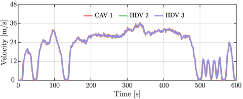
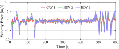
(a) All HDVs

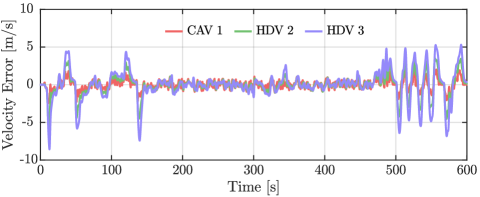
(b) Standard MPC

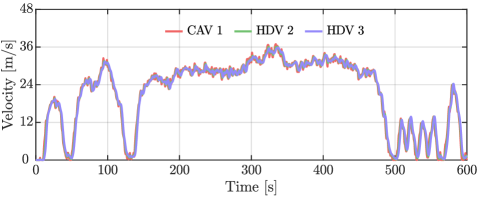
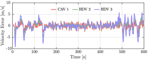
(c) Standard DeeP-LCC

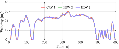
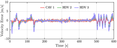
(d) RDeeP-LCC

Figure 3: Velocity profiles and tracking velocity errors in mixed platoon simulation results under four conditions: all vehicles are HDVs, standard MPC, standard DeeP-LCC, and RDeeP-LCC. The red profiles represent the CAV (indexed as 1), the green profiles represent HDV (indexed as 2), and the purple profiles represent HDV (indexed as 3). Both standard DeeP-LCC and RDeeP-LCC use the same dataset.

The simulation results for our RDeeP-LCC method, and the baseline methods (all HDVs, standard MPC, and standard DeeP-LCC), are depicted in Figure 3. For brevity, we only present the results under a noise boundary $\omega_{\mathrm{max}}=0.02$ and an attack boundary $\vartheta_{\mathrm{max}}=2$. The left subgraphs in Figure3(a)-(d) illustrate that overall, all methods enable the mixed platoon to track the head vehicle’s velocity. However, there are slight differences in the velocity profiles. To provide more detailed insights, the corresponding velocity errors are shown in the right subgraphs of Figure3(a)-(d), respectively.

From the velocity error perspective, the methods involving all vehicles are HDVs, standard DeeP-LCC, or standard MPC exhibit significant error amplification during strong acceleration or deceleration of the head vehicle (at about $10\text{\,}\mathrm{s}$, $130\text{\,}\mathrm{s}$, and $$500\text{\,}\mathrm{s}$-$600\text{\,}\mathrm{s}$$), as shown in Figure3(a)-(c). In contrast, the velocity error is reduced when the CAV employs RDeeP-LCC, as shown in Figure3(d). This reduction highlights the effectiveness of RDeeP-LCC in mitigating the impact of process noise and attack inputs.

It is important to note that different levels of noise and attack can significantly affect controller performance. To investigate sensitivity to these factors, we conduct $10$ simulation tests for each combination of noise boundary $\omega_{\mathrm{max}}$ and attack boundary $\vartheta_{\mathrm{max}}$. In order to quantify the performance of our method and other baseline methods under different noise boundaries $\omega_{\mathrm{max}}$ and attack boundaries $\vartheta_{\mathrm{max}}$, we adopt the velocity mean absolute deviation $R_{\mathrm{v}}$ as index a performance index for tracking [58], defined as follows:

$$R_{\mathrm{v}}=\frac{1}{(t_{\mathrm{f}}-t_{\mathrm{0}})}\frac{1}{n}\sum_{k=t_{\mathrm{0}}}^{t_{\mathrm{f}}}\sum_{i=1}^{n}\left|v_{i}(k)-{v}^{*}(k)\right|,$$ (48)

where $t_{\mathrm{0}}$ and $t_{\mathrm{f}}$ are the start and end time steps, respectively.

In addition, based on (35), we apply the real cost value $R_{\mathrm{c}}$ obtained at each simulation under different control methods to quantify the control performance, expressed as follows:

$$R_{\mathrm{c}}=\sum_{k=t_{\mathrm{0}}}^{t_{\mathrm{f}}}\left(\|x(k)\|_{Q}^{2}+\|u(k)\|_{R}^{2}\right).$$ (49)

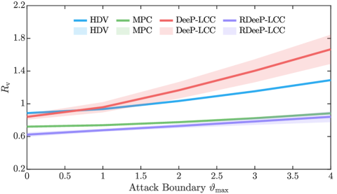
(a) Velocity mean absolute velocity deviation $R_{\mathrm{v}}$

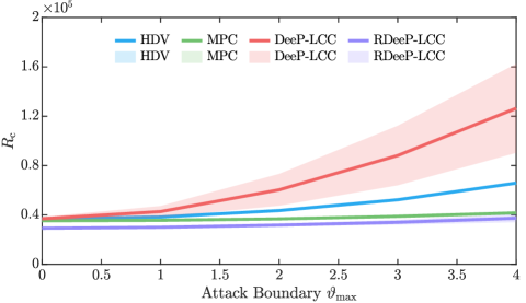
(b) Real cost value $R_{\mathrm{c}}$

Figure 4: The values of $R_{\mathrm{v}}$ and $R_{\mathrm{c}}$ for multiple simulations under all the vehicles are HDVs, standard MPC, standard DeeP-LCC, and RDeeP-LCC. The dark-colored solid lines represent the mean values of $R_{\mathrm{v}}$ and $R_{\mathrm{c}}$ across multiple simulations, and the light-colored shaded areas depict the mean $\pm$ standard deviation.

Figure 4 presents the values of $R_{\mathrm{v}}$ and $R_{\mathrm{c}}$ for simulations conducted under different control methods. In Figure 4(a), both standard MPC and RDeeP-LCC exhibit smaller mean values for $R_{\mathrm{v}}$ compared to all-HDV configuration across varying $\omega_{\mathrm{max}}$ and $\vartheta_{\mathrm{max}}$ conditions. Notably, RDeeP-LCC achieves the lowest mean $R_{\mathrm{v}}$ values. Higher values of $R_{\mathrm{v}}$ indicate greater velocity error, reflecting a reduced capability of the CAVs to track the head vehicle accurately. These results highlight the superiority of the proposed RDeeP-LCC method over standard MPC in mixed platoon velocity tracking performance, significantly outperforming the all-HDV configuration. It is noteworthy that for standard DeeP-LCC, $R_{\mathrm{v}}$ value is lower than that of all-HDV configuration only when approximately $\vartheta_{\mathrm{max}}\leq 0.5$. Under higher attack boundaries, the standard DeeP-LCC exhibits higher $R_{\mathrm{v}}$ values than all-HDV configuration, indicating its lack of robustness against process noise and attacks without specific robust design.

Furthermore, Figure 4(b) illustrates the real cost values $R_{\mathrm{c}}$ in (49) for our RDeeP-LCC method and baseline methods. The results clearly show that our RDeeP-LCC method consistently achieves the lowest cost values $R_{\mathrm{c}}$ values across different conditions. This advantage is due to our emphasis on noise and attack mitigation through reachability set analysis, which maintains tighter state constraints for the mixed platoon system, thus ensuring robustness in dynamic environments. While standard MPC shows lower $R_{\mathrm{c}}$ values than all HDVs, it lacks specific considerations for attack mitigation, resulting in higher $R_{\mathrm{c}}$ values compared to our method and diminished robustness under significant attack conditions. Notably, for the standard DeeP-LCC method, its $R_{\mathrm{c}}$ remains low when attacks are absent. However, as noise and attack increase, its performance becomes unacceptable, with the mean $R_{\mathrm{c}}$ value reaching $1.2\text{\,}\times\mathrm{1}\mathrm{0}^{5}$ when $\vartheta_{\mathrm{max}}=4$. This performance degradation is attributed to the heavy reliance of the standard DeeP-LCC on data for modeling (42), where the presence of data noise significantly reduces model accuracy. Additionally, standard DeeP-LCC lacks preemptive robustness against attacks, further compromising its control performance in environments with coexisting noise and attacks. In contrast, our proposed RDeeP-LCC method demonstrates enhanced robustness against noise and attacks, ensuring reliable mixed platoon control. By integrating reachability set analysis into the data-driven control framework, our method effectively addresses the challenges posed by noise and attacks, making it a promising solution for real-world applications where robustness is crucial.

V Human-in-the-Loop Experiment

In this section, we establish a human-in-the-loop bench experimental platform to verify the effectiveness of the RDeeP-LCC method proposed in this paper.

V-A Human-in-the-Loop Experimental Platform

To validate the effectiveness of the RDeeP-LCC method under process noise and adversarial attacks, we developed a human-in-the-loop platform to replicate a real driving scenario. As depicted in Figure 5, the setup comprises a visualization screen module, two Logitech G29 driving simulator modules (including brake pedal, accelerator pedal, and steering wheel), USB 3.0 communication modules, and the mainframe computing module, whose programs run on the cloud server.

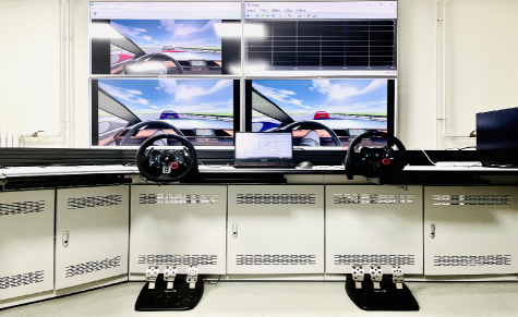
Figure 5: Human-in-the-loop experimental platform for mixed platoon control.

Drivers monitor the dynamics of the preceding vehicles through a high-definition visualization screen module and precisely control the vehicle using the Logitech G29 simulators. The Logitech G29 simulators connect to the mainframe computing module via the USB 3.0 protocol, transmitting real-time control commands from the drivers, including braking, acceleration, and steering maneuvers. These commands are then relayed to the PreScan software, which displays the vehicle dynamics in real-time on the visualization screen. The control algorithms and detailed model of the simulated vehicle (including the engine, transmission, and gears) are developed within the Matlab/Simulink environment. In addition, we use the uniform random number module in Simulink to simulate noise and attacks, reproducing realistic driving conditions.

V-B Experimental Design

Utilizing the human-in-the-loop platform, we conduct experimental validation of the RDeeP-LCC method proposed in this paper, alongside standard MPC and standard DeeP-LCC. In our experiments, the RDeeP-LCC method or other baseline methods control the CAV (indexed as 1), while two drivers operate the HDVs (indexed as 2 and 3) using the Logitech G29 simulators. To ensure accuracy and consistency, before the formal experiment, drivers undergo a $3$-hour training session in car-following scenarios to familiarize themselves with the driving simulators. To replicate a realistic traffic scenario, the head vehicle (indexed as $0$) is assigned a time-varying velocity profile derived from the SFTP-US06 driving cycle, while subject to a noise boundary of $\omega_{\mathrm{max}}=0.02$ and an attack boundary of $\vartheta_{\mathrm{max}}=2$. All other experimental configurations are consistent with the simulation settings outlined in Section IV.

In this experiment, we initially set the velocity of the head vehicle as the equilibrium velocity $v^{*}_{i}$. It is important to note that unlike the OVM model (45) utilized by HDVs in Section IV, where equilibrium spacing $s^{*}_{i}$ can can be directly calculated from $v^{*}_{i}$ based on (46) and (47) during the simulation. However, it is a challenge for us to get the equilibrium spacing $s^{*}_{i}$ for real drives. To address this issue, we conduct a preliminary experiment where two drivers operate their vehicles in a car-following scenario using the SFTP-US06 driving cycle. Subsequently, we gather experimental data, represented by the green points in Figure 6. This data is then utilized to fit the HDVs model using the OVM model (46) and (47) as the foundation for MPC. The fitting results for two drivers, namely HDV $2$ and HDV $3$, are illustrated by the purple lines in Figure 6(a) and (b), respectively. The parameters obtained from the fitting process for the two drivers are as follows: for HDV $2$, $v_{\max}=36$, $s_{\min}=4.6$, $s_{\max}=30.6$; for HDV $3$, $v_{\max}=36$, $s_{\min}=7.5$, $s_{\max}=49.4$. By employing the fitted model, we are able to make estimations regarding the equilibrium spacing $s^{*}_{i}$ in the online predictive control phase.

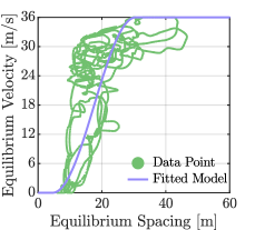
(a) Fitting results for HDV $2$

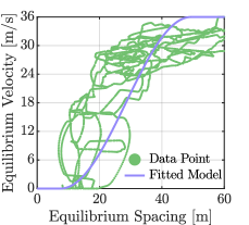
(b) Fitting results for HDV $3$

Figure 6: The fitting results of equilibrium spacings and equilibrium velocities for the two HDVs. The green points represent the collected data, and the purple lines represent the relationship between equilibrium spacings and equilibrium velocities fitted using the OVM framework.

In the formal experiments for method validation, we first conduct data collection of the mixed platoon. The data collection settings are the same as in Section IV, except that real human drivers are used. In the offline phase, based on the pre-collected data, we proceed with the construction of the matrix zonotope set $\mathcal{M}_{ABHJ}$ in (19), the feedback control law $K$ in (26), and the Hankel matrices in (28), as outlined in Section IV. Subsequently, we transition to the online predictive control phase. Here, the head vehicle initiates its motion according to the predefined profile, while the CAV and two HDVs respond to the controller’s commands and the drivers’ actions, respectively. Upon completion of the trial, experimental data are gathered for subsequent analysis. The settings for this phase align with those detailed in Section IV.

V-C Experimental Results

The experimental results comparing the algorithm proposed in this study with other baseline methods are presented in Figure 7. In the presence of noise and attacks, significant velocity tracking errors are observed in all HDVs, as illustrated in Figure 7(a), indicating inadequate tracking performance for all HDV scenarios. Notably, the standard DeeP-LCC method shows more pronounced velocity tracking errors than all HDVs, as depicted in Figure 7(c). These errors stem from the DeeP-LCC method’s lack of tailored approaches to address noise and attack issues. Specifically, noise disrupts the data-driven dynamic model, while attacks directly impact the CAV’s dynamic behavior, resulting in decreased tracking accuracy. In contrast, both the standard MPC method and the RDeeP-LCC method have effectively improved the tracking performance of the mixed platoon. Furthermore, a comparison between Figure 7(b) and Figure 7(d) reveals that the vehicles’ tracking error in the RDeeP-LCC method is even smaller, as indicated by the lines in Figure 7(d). This outcome underscores the exceptional tracking performance of the RDeeP-LCC method, highlighting its robustness and efficacy in achieving precise control under diverse traffic conditions.

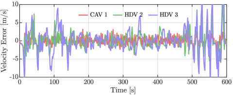
(a) All HDVs

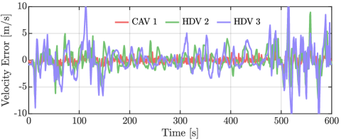
(b) Standard MPC

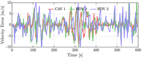
(c) Standard DeeP-LCC

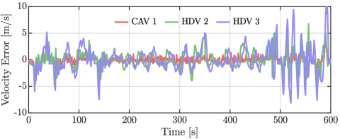
(d) RDeeP-LCC

Figure 7: Velocity errors in mixed platoon human-in-the-loop experimental under all vehicles are HDVs, standard MPC, standard DeeP-LCC, and RDeeP-LCC. The red, green, and purple profiles represent the CAV (indexed as 1) and the HDVs (indexed as 2, 3), respectively. Here, standard DeeP-LCC and RDeeP-LCC use the same dataset.

To comprehensively evaluate the performance of the different controllers, three experiments are carried out for each controller type. Subsequently, we compute the average performance indices $R_{\mathrm{v}}$ and $R_{\mathrm{c}}$ using (48) and (49). The average values of $R_{\mathrm{v}}$ and $R_{\mathrm{c}}$ are presented in Table I for comparison. Table I provides a detailed list of the two indices, $R_{\mathrm{v}}$ and $R_{\mathrm{c}}$, which intuitively reflect the control performance of velocity tracking. The research results suggest that, compared to all other baseline methods, the RDeeP-LCC method proposed in this study demonstrates a notable superiority in control performance. Specifically, compared with the all HDVs, the RDeeP-LCC method achieves significant enhancements of $26.1\text{\,}\%$ and $24.7\text{\,}\%$ in the $R_{\mathrm{v}}$ and $R_{\mathrm{c}}$ indices, respectively. This success serves to validate the practicality and efficacy of our approach. Conversely, compared to all HDVs, the standard MPC method only yielded improvements of $18.8\text{\,}\%$ and $16.5\text{\,}\%$ in the $R_{\mathrm{v}}$ and $R_{\mathrm{c}}$ indices, respectively. It is important to highlight that the standard DeeP-LCC method shows the highest values in the $R_{\mathrm{v}}$ and $R_{\mathrm{c}}$ indices. This implies that predictive control approaches based solely on data-driven techniques, without explicit robust design considerations, may struggle to meet desired tracking performance standards in the presence of process noise and attacks. In fact, such approaches might even exhibit worse performance compared to the inherent capabilities of all HDVs. In contrast, our innovative approach focuses on optimizing constraints using reachable set analysis, seeking to ensure that the state of a mixed platoon system remains within a tighter set of safety constraints. By adopting this strategy, the robustness of mixed platoon control systems is significantly enhanced against the adverse effects of process noise and attacks.

TABLE I: Performance Indices in Human-in-the-loop Experiment

Index	All HDVs	MPC	DeeP-LCC	RDeeP-LCC
$R_{\mathrm{v}}$	$1.65$	$1.34$	$2.40$	$1.22$
	$(--)$	$(\downarrow$18.8\text{\,}\%$)$	$(\uparrow$45.5\text{\,}\%$)$	$(\downarrow$26.1\text{\,}\%$)$
$R_{\mathrm{c}}$	$0.97\times 10^{6}$	$0.81\times 10^{6}$	$3.53\times 10^{6}$	$0.73\times 10^{6}$
	$(--)$	$(\downarrow$16.5\text{\,}\%$)$	$(\uparrow$263.9\text{\,}\%$)$	$(\downarrow$24.7\text{\,}\%$)$

VI Conclusion

In this paper, we propose a novel RDeeP-LCC method for mixed platoon control under conditions of data noise and adversarial attacks. The RDeeP-LCC method incorporates the unknown dynamics for HDVs and directly relies on trajectory data of mixed platoons to construct data-driven reachable set constraints and a data-driven predictive controller, which provides safe and robust control inputs for CAVs. To validate the effectiveness and superiority of this method, both numerical simulations and human-in-the-loop experiments are conducted. The results indicate that the RDeeP-LCC method has significantly improved the tracking performance of mixed platoons in the presence of data noise and adversarial attacks.

In future research, one practical concern in RDeeP-LCC is the influence of communication delays induced by actuators and communication. Existing studies have shown the potential of standard DeeP-LCC in addressing delay issues [59], but there is still a lack of customized data-driven control strategies for delay problems. Another interesting topic is to improve the real-time computational efficiency of data-driven predictive control methods, which facilitates scalable deployment in real-world traffic scenarios.

References

- [1] J. C. De Winter, R. Happee, M. H. Martens, and N. A. Stanton, “Effects of adaptive cruise control and highly automated driving on workload and situation awareness: A review of the empirical evidence,” Transportation research part F: traffic psychology and behaviour, vol. 27, pp. 196–217, 2014.
- [2] Y. Luo, T. Chen, S. Zhang, and K. Li, “Intelligent hybrid electric vehicle acc with coordinated control of tracking ability, fuel economy, and ride comfort,” IEEE Transactions on Intelligent Transportation Systems, vol. 16, no. 4, pp. 2303–2308, 2015.
- [3] G. Gunter, D. Gloudemans, R. E. Stern, S. McQuade, R. Bhadani, M. Bunting, M. L. Delle Monache, R. Lysecky, B. Seibold, J. Sprinkle et al., “Are commercially implemented adaptive cruise control systems string stable?” IEEE Transactions on Intelligent Transportation Systems, vol. 22, no. 11, pp. 6992–7003, 2020.
- [4] M. Makridis, K. Mattas, B. Ciuffo, F. Re, A. Kriston, F. Minarini, and G. Rognelund, “Empirical study on the properties of adaptive cruise control systems and their impact on traffic flow and string stability,” Transportation research record, vol. 2674, no. 4, pp. 471–484, 2020.
- [5] M. Shen and G. Orosz, “Data-driven predictive connected cruise control,” in 2023 IEEE Intelligent Vehicles Symposium (IV). IEEE, 2023, pp. 1–6.
- [6] S. Öncü, J. Ploeg, N. Van de Wouw, and H. Nijmeijer, “Cooperative adaptive cruise control: Network-aware analysis of string stability,” IEEE Transactions on Intelligent Transportation Systems, vol. 15, no. 4, pp. 1527–1537, 2014.
- [7] S. W. Smith, Y. Kim, J. Guanetti, R. Li, R. Firoozi, B. Wootton, A. A. Kurzhanskiy, F. Borrelli, R. Horowitz, and M. Arcak, “Improving urban traffic throughput with vehicle platooning: Theory and experiments,” IEEE Access, vol. 8, pp. 141 208–141 223, 2020.
- [8] F. Ma, Y. Yang, J. Wang, Z. Liu, J. Li, J. Nie, Y. Shen, and L. Wu, “Predictive energy-saving optimization based on nonlinear model predictive control for cooperative connected vehicles platoon with v2v communication,” Energy, vol. 189, p. 116120, 2019.
- [9] D. Hajdu, I. G. Jin, T. Insperger, and G. Orosz, “Robust design of connected cruise control among human-driven vehicles,” IEEE Transactions on Intelligent Transportation Systems, vol. 21, no. 2, pp. 749–761, 2019.
- [10] Y. Jiang, F. Zhu, Z. Yao, Q. Gu, B. Ran et al., “Platoon intensity of connected automated vehicles: Definition, formulas, examples, and applications,” Journal of Advanced Transportation, vol. 2023, 2023.
- [11] I. G. Jin and G. Orosz, “Optimal control of connected vehicle systems with communication delay and driver reaction time,” IEEE Transactions on Intelligent Transportation Systems, vol. 18, no. 8, pp. 2056–2070, 2016.
- [12] C. Chen, J. Wang, Q. Xu, J. Wang, and K. Li, “Mixed platoon control of automated and human-driven vehicles at a signalized intersection: dynamical analysis and optimal control,” Transportation research part C: emerging technologies, vol. 127, p. 103138, 2021.
- [13] J. Yang, D. Zhao, J. Lan, S. Xue, W. Zhao, D. Tian, Q. Zhou, and K. Song, “Eco-driving of general mixed platoons with cavs and hdvs,” IEEE Transactions on Intelligent Vehicles, vol. 8, no. 2, pp. 1190–1203, 2022.
- [14] R. E. Stern, S. Cui, M. L. Delle Monache, R. Bhadani, M. Bunting, M. Churchill, N. Hamilton, H. Pohlmann, F. Wu, B. Piccoli et al., “Dissipation of stop-and-go waves via control of autonomous vehicles: Field experiments,” Transportation Research Part C: Emerging Technologies, vol. 89, pp. 205–221, 2018.
- [15] J. Wang, Y. Zheng, Q. Xu, J. Wang, and K. Li, “Controllability analysis and optimal control of mixed traffic flow with human-driven and autonomous vehicles,” IEEE Transactions on Intelligent Transportation Systems, vol. 22, no. 12, pp. 7445–7459, 2020.
- [16] C. Wu, A. R. Kreidieh, K. Parvate, E. Vinitsky, and A. M. Bayen, “Flow: A modular learning framework for mixed autonomy traffic,” IEEE Transactions on Robotics, vol. 38, no. 2, pp. 1270–1286, 2021.
- [17] J. Zhan, Z. Ma, and L. Zhang, “Data-driven modeling and distributed predictive control of mixed vehicle platoons,” IEEE Transactions on Intelligent Vehicles, vol. 8, no. 1, pp. 572–582, 2022.
- [18] J. Guo, H. Guo, J. Liu, D. Cao, and H. Chen, “Distributed data-driven predictive control for hybrid connected vehicle platoons with guaranteed robustness and string stability,” IEEE Internet of Things Journal, vol. 9, no. 17, pp. 16 308–16 321, 2022.
- [19] J. Wang, Y. Zheng, J. Dong, C. Chen, M. Cai, K. Li, and Q. Xu, “Implementation and experimental validation of data-driven predictive control for dissipating stop-and-go waves in mixed traffic,” IEEE Internet of Things Journal, 2023.
- [20] I. G. Jin, S. S. Avedisov, C. R. He, W. B. Qin, M. Sadeghpour, and G. Orosz, “Experimental validation of connected automated vehicle design among human-driven vehicles,” Transportation research part C: emerging technologies, vol. 91, pp. 335–352, 2018.
- [21] M. Treiber, A. Hennecke, and D. Helbing, “Congested traffic states in empirical observations and microscopic simulations,” Physical review E, vol. 62, no. 2, p. 1805, 2000.
- [22] M. Bando, K. Hasebe, A. Nakayama, A. Shibata, and Y. Sugiyama, “Dynamical model of traffic congestion and numerical simulation,” Physical review E, vol. 51, no. 2, p. 1035, 1995.
- [23] S. Feng, Z. Song, Z. Li, Y. Zhang, and L. Li, “Robust platoon control in mixed traffic flow based on tube model predictive control,” IEEE Transactions on Intelligent Vehicles, vol. 6, no. 4, pp. 711–722, 2021.
- [24] Y. Wang, S. Lin, Y. Wang, B. De Schutter, and J. Xu, “Robustness analysis of platoon control for mixed types of vehicles,” IEEE Transactions on Intelligent Transportation Systems, vol. 24, no. 1, pp. 331–340, 2022.
- [25] C. Zhao, H. Yu, and T. G. Molnar, “Safety-critical traffic control by connected automated vehicles,” Transportation research part C: emerging technologies, vol. 154, p. 104230, 2023.
- [26] W. Gao, Z.-P. Jiang, and K. Ozbay, “Data-driven adaptive optimal control of connected vehicles,” IEEE Transactions on Intelligent Transportation Systems, vol. 18, no. 5, pp. 1122–1133, 2016.
- [27] M. Huang, Z.-P. Jiang, and K. Ozbay, “Learning-based adaptive optimal control for connected vehicles in mixed traffic: robustness to driver reaction time,” IEEE transactions on cybernetics, vol. 52, no. 6, pp. 5267–5277, 2020.
- [28] E. Vinitsky, K. Parvate, A. Kreidieh, C. Wu, and A. Bayen, “Lagrangian control through deep-rl: Applications to bottleneck decongestion,” in 2018 21st International Conference on Intelligent Transportation Systems (ITSC). IEEE, 2018, pp. 759–765.
- [29] J. Lan, D. Zhao, and D. Tian, “Safe and robust data-driven cooperative control policy for mixed vehicle platoons,” International Journal of Robust and Nonlinear Control, vol. 33, no. 7, pp. 4171–4190, 2023.
- [30] J. Zhou, L. Yan, and K. Yang, “Safe reinforcement learning for mixed-autonomy platoon control,” in 2023 IEEE 26th International Conference on Intelligent Transportation Systems (ITSC). IEEE, 2023, pp. 5744–5749.
- [31] ——, “Enhancing system-level safety in mixed-autonomy platoon via safe reinforcement learning,” arXiv preprint arXiv:2401.11148, 2024.
- [32] L. Hewing, K. P. Wabersich, M. Menner, and M. N. Zeilinger, “Learning-based model predictive control: Toward safe learning in control,” Annual Review of Control, Robotics, and Autonomous Systems, vol. 3, pp. 269–296, 2020.
- [33] J. Lan, D. Zhao, and D. Tian, “Data-driven robust predictive control for mixed vehicle platoons using noisy measurement,” IEEE Transactions on Intelligent Transportation Systems, vol. 24, no. 6, pp. 6586–6596, 2021.
- [34] J. Wang, Y. Zheng, K. Li, and Q. Xu, “Deep-lcc: Data-enabled predictive leading cruise control in mixed traffic flow,” IEEE Transactions on Control Systems Technology, 2023.
- [35] Y. Wu, Z. Zuo, Y. Wang, and Q. Han, “Driver-centric data-driven robust model predictive control for mixed vehicular platoon,” Nonlinear Dynamics, pp. 1–15, 2023.
- [36] J. Coulson, J. Lygeros, and F. Dörfler, “Data-enabled predictive control: In the shallows of the deepc,” in 2019 18th European Control Conference (ECC). IEEE, 2019, pp. 307–312.
- [37] J. C. Willems, P. Rapisarda, I. Markovsky, and B. L. De Moor, “A note on persistency of excitation,” Systems & Control Letters, vol. 54, no. 4, pp. 325–329, 2005.
- [38] J. Wang, Y. Zheng, C. Chen, Q. Xu, and K. Li, “Leading cruise control in mixed traffic flow: System modeling, controllability, and string stability,” IEEE Transactions on Intelligent Transportation Systems, vol. 23, no. 8, pp. 12 861–12 876, 2021.
- [39] D. Li, K. Zhang, H. Dong, Q. Wang, Z. Li, and Z. Song, “Physics-augmented data-enabled predictive control for eco-driving of mixed traffic considering diverse human behaviors,” IEEE Transactions on Control Systems Technology, 2024.
- [40] K. Zhang, K. Chen, Z. Li, J. Chen, and Y. Zheng, “Privacy-preserving data-enabled predictive leading cruise control in mixed traffic,” IEEE Transactions on Intelligent Transportation Systems, 2023.
- [41] Q. Xu, Y. Liu, J. Pan, J. Wang, J. Wang, and K. Li, “Reachability analysis plus satisfiability modulo theories: An adversary-proof control method for connected and autonomous vehicles,” IEEE Transactions on Industrial Electronics, vol. 70, no. 3, pp. 2982–2992, 2022.
- [42] C. Zhao and H. Yu, “Robust safety for mixed-autonomy traffic with delays and disturbances,” arXiv preprint arXiv:2310.04007, 2023.
- [43] L. Huang, J. Zhen, J. Lygeros, and F. Dörfler, “Robust data-enabled predictive control: Tractable formulations and performance guarantees,” IEEE Transactions on Automatic Control, vol. 68, no. 5, pp. 3163–3170, 2023.
- [44] J. Berberich, J. Köhler, M. A. Müller, and F. Allgöwer, “Data-driven model predictive control with stability and robustness guarantees,” IEEE Transactions on Automatic Control, vol. 66, no. 4, pp. 1702–1717, 2020.
- [45] X. Shang, J. Wang, and Y. Zheng, “Smoothing mixed traffic with robust data-driven predictive control for connected and autonomous vehicles,” arXiv preprint arXiv:2310.00509, 2023.
- [46] B. Schürmann, M. Klischat, N. Kochdumper, and M. Althoff, “Formal safety net control using backward reachability analysis,” IEEE Transactions on Automatic Control, vol. 67, no. 11, pp. 5698–5713, 2021.
- [47] S. Li, C. Chen, H. Zheng, J. Wang, Q. Xu, and K. Li, “Robust data-enabled predictive leading cruise control via reachability analysis,” arXiv preprint arXiv:2402.03897, 2024.
- [48] A. Alanwar, A. Koch, F. Allgöwer, and K. H. Johansson, “Data-driven reachability analysis from noisy data,” IEEE Transactions on Automatic Control, 2023.
- [49] X. Jin, W. M. Haddad, Z.-P. Jiang, and K. G. Vamvoudakis, “Adaptive control for mitigating sensor and actuator attacks in connected autonomous vehicle platoons,” in 2018 IEEE Conference on Decision and Control (CDC). IEEE, 2018, pp. 2810–2815.
- [50] M. Althoff, “Reachability analysis and its application to the safety assessment of autonomous cars,” Ph.D. dissertation, Technische Universität München, 2010.
- [51] W. Kühn, “Rigorously computed orbits of dynamical systems without the wrapping effect,” Computing, vol. 61, pp. 47–67, 1998.
- [52] H. J. Van Waarde, M. K. Camlibel, J. Eising, and H. L. Trentelman, “Quadratic matrix inequalities with applications to data-based control,” SIAM Journal on Control and Optimization, vol. 61, no. 4, pp. 2251–2281, 2023.
- [53] D. Q. Mayne, M. M. Seron, and S. V. Raković, “Robust model predictive control of constrained linear systems with bounded disturbances,” Automatica, vol. 41, no. 2, pp. 219–224, 2005.
- [54] C. Fan, U. Mathur, S. Mitra, and M. Viswanathan, “Controller synthesis made real: Reach-avoid specifications and linear dynamics,” in International Conference on Computer Aided Verification. Springer, 2018, pp. 347–366.
- [55] J. Wang, Y. Lian, Y. Jiang, Q. Xu, K. Li, and C. N. Jones, “Distributed data-driven predictive control for cooperatively smoothing mixed traffic flow,” Transportation Research Part C: Emerging Technologies, vol. 155, p. 104274, 2023.
- [56] M. Althoff, “Guaranteed state estimation in cora 2021,” in Proc. of the 8th International Workshop on Applied Verification of Continuous and Hybrid Systems, 2021.
- [57] T. G. Reid, S. E. Houts, R. Cammarata, G. Mills, S. Agarwal, A. Vora, and G. Pandey, “Localization requirements for autonomous vehicles,” SAE International Journal of Connected and Automated Vehicles, vol. 2, no. 12-02-03-0012, pp. 173–190, 2019.
- [58] M. Kamrani, R. Arvin, and A. J. Khattak, “Extracting useful information from basic safety message data: An empirical study of driving volatility measures and crash frequency at intersections,” Transportation research record, vol. 2672, no. 38, pp. 290–301, 2018.
- [59] L. Huang, J. Coulson, J. Lygeros, and F. Dörfler, “Decentralized data-enabled predictive control for power system oscillation damping,” IEEE Transactions on Control Systems Technology, vol. 30, no. 3, pp. 1065–1077, 2021.