Hybrid Physics-ML Modeling for Marine Vehicle Maneuvering Motions in the Presence of Environmental Disturbances

Abstract

A hybrid physics-machine learning modeling framework is proposed for the surface vehicles’ maneuvering motions to address the modeling capability and stability in the presence of environmental disturbances. From a deep learning perspective, the framework is based on a variant version of residual networks with additional feature extraction. Initially, an imperfect physical model is derived and identified to capture the fundamental hydrodynamic characteristics of marine vehicles. This model is then integrated with a feedforward network through a residual block. Additionally, feature extraction from trigonometric transformations is employed in the machine learning component to account for the periodic influence of currents and waves. The proposed method is evaluated using real navigational data from the ’JH7500’ unmanned surface vehicle. The results demonstrate the robust generalizability and accurate long-term prediction capabilities of the nonlinear dynamic model in specific environmental conditions. This approach has the potential to be extended and applied to develop a comprehensive high-fidelity simulator.

I Introduction

In the development of autonomous surface vehicle techniques, high-fidelity models of maneuvering motions are critical for providing comprehensive mission simulations, validating real-time control systems, and developing reinforcement learning-based algorithms. Given the inherent risk and expense associated with physical testing on actual vessels, developing a realistic simulator is cost-efficient to provide extensive simulated experience. To enhance the realism of vehicle simulators, it is essential to integrate ship maneuvering models that mirror the actual kinetic characteristics. Specifically, this requires the model to accurately simulate the vehicle’s nonlinear behavior when encountering environmental disturbances during the operational phase.

However, conventional ship maneuvering modeling theories primarily focus on assessing maneuverability at the early design phase. These methods generally derive explicit formulas based on first-principles theory and obtain parameters through captive model tests, empirical formula calculations, or numerical calculations. Although widely used by the industry, these methods heavily rely on specialized facilities, basins, or computational resources, which are economically and time-costly. Moreover, due to scale effects and simplifications in the models, they often deviate from the actual kinetic characteristics during the operational phase.

To fulfill the need for mirroring actual ship kinetics, one feasible approach is to establish models utilizing actual navigational data, as such data contain up-to-date information on the actual kinetic characteristics. These methods are referred to as the data-driven method, also known as system identification in the control field. In contrast to the conventional methods mentioned above, the data-driven method can be applied to full-scale ships and has the potential for real-time updating. These two advantages make it more suitable for the operational phase.

In the field of ship kinetic modeling, parametric modeling was initially a commonly used data-driven method. This method focuses on estimating hydrodynamic derivatives from free-running test data. Similar to captive model tests, it relies on a prior model structure derived from first principles. For clarity and to guide the subsequent discussion, this study uses the term physical model to define this class of models built using model structure as prior knowledge. This process often requires extraordinary effort and expertise to determine the model structure in pursuit of precision. However, although these models are formulated based on physical laws, in most cases, they are inevitably approximations of reality due to incomplete knowledge of certain processes, which introduces bias.

In contrast to the physical model, another class of data-driven approaches employs non-parametric modeling to create a pure data-driven model, which maps inputs to outputs without any prior physical assumptions. Machine learning (ML) techniques have offered a range of advanced algorithms for effectively modeling nonlinear ship dynamics. However, the application of black-box machine learning in engineering domains is subject to inherent limitations for several reasons: (i) Firstly, while state-of-the-art machine learning models excel at capturing complex dynamic characteristics, they necessitate a larger volume of data compared to physics-based modeling. (ii) Additionally, they are more susceptible to noise, which can result in changes to the model complexity; thereby requiring higher data quality. In practice, obtaining clean data in completely still water is a rare occurrence. (iii) Thirdly, machine learning models can only capture the characteristics present in the training data and therefore lack the ability to generalize to out-of-sample scenarios.

To overcome these limitations, a hybrid approach that combines ML techniques with physics-based modeling can be beneficial. This paper presents a hybrid physical-ML modeling approach that learns vessel kinetics under environmental influences. The effectiveness of the proposed approach is validated with experimental data from the ’Jing Hai’ unmanned surface vehicle. By incorporating domain knowledge and physical laws into the modeling process, the resulting models can be more interpretable, generalizable, and robust.

This study makes two main contributions: (i) A specialized hybrid physical-ML strategy that integrates the stability and constraint benefits of the physical model with the advanced predictive capabilities of the ML model. This integration allows for precise predictions in specific environmental conditions even without direct environmental data. (ii) A focus on maneuver-level motion modeling under environmental disturbances, providing a precise characterization of vessel maneuverability. This focus differs from previous studies that emphasize sustained predictions for large vessels over voyages.

The structure of this paper is as follows: Section II provides an overview of the related work. Section III presents a detailed explanation of the methodology behind the hybrid modeling framework. Section IV conducts a comprehensive analysis of the proposed method using experimental data. Finally, conclusions are drawn in Section V.

II Related Work

II-A Physical Model

Physical Models are developed by formulating mathematical equations based on physical principles and determining unknown parameters within these equations, such as the Abkowitz model[1] and the MMG model[2]. One primary challenge lies in the concrete representation of the hydrodynamic forces and moments. Typically, they are formulated as 3rd-order polynomial or 2nd-order quasi-polynomial functions of kinematic parameters and sometimes of rudder angles, derived from Taylor series expansions. However, the accurate expression of hydrodynamic characteristics is nontrivial and necessitates the application of expert knowledge and domain-specific insights for appropriate fine-tuning.

Once the model structure is determined, the focus shifts to obtaining unknown hydrodynamic derivatives. For the data-driven approaches based on free-running test data, estimating a large number of parameters often leads to parameter drift and poor generalization problems. Techniques like ridge regression [3], support vector regression [4] are utilized to control model complexity and mitigate overfitting risks. Moreover, methods like Bayesian methods [5], fuzzy neural networks [6], the event-triggered robust UKF [7], among others are also considered. However, the challenge still exists for analyzing the interactions between ship hulls and actual environmental disturbances. Due to the complexity of the physical mechanisms, the predictive models for the operational phase remain to be developed.

II-B Pure Data-Driven Model

The pure data-driven model directly establishes ship maneuvering models by learning the nonlinear mapping between input and output data, without relying heavily on domain knowledge or prior assumptions. The development of machine learning technologies has provided advanced algorithms for this approach to modeling ship dynamics. Representative methods include kernel-based methods [8, 9, 10], neural network methods[11], dynamic mode decomposition [12], and others.

He et al.[11] designed a self-designed fully connected neural network for non-parametric modeling of ship maneuvering, demonstrating that a three-degree-of-freedom model can be built using a simple network structure within three hidden layers. In recent years, time series forecasting methods are utilized to predict ship maneuvering motions, such as recurrent neural networks [13] and long-short-term-memory (LSTM) deep neural networks [14]. In addition, Zhang et al.[15] proposed a multi-scale attention mechanism to enhance the performance of LSTM in ship motion prediction. Dong et al.[16] introduced an attention mechanism model based on positional encoding to quantify the temporal correlation of ship maneuvering motions.

To explore real-world scenarios, Wang et al. [17] employed DNN, RNN, LSTM, and GRU to construct nonparametric models based on real voyage data, with DNN showing slightly better performance. They claim that applying nonparametric modeling using real voyage data is challenging, requiring attention to numerous details. Jang et al. [18] conducted a study on multistep predictions for surface vehicles using a temporal segment-based network in a canal environment. Wang et al. [19] introduced a multi-layer neural network incorporating multistep constraints in the loss function. Impressively, Lou et al.[20] presented a deep learning network and focused on the predictions of turning tests. This paper offers valuable insights on utilizing trigonometric features to address the lack of reliable environmental measurement, whereas it lacks a detailed discussion on the generalizability validation of the method.

II-C Hybrid Model

Some scholars have developed hybrid models by integrating physics-based models and ML models within a framework. This integration aims to leverage the strengths of both models, utilizing the physical understanding of the physics-based model while benefiting from the data-driven capabilities and adaptability of the machine learning model [21].

One method that has garnered attention is residual modeling, also known as parallel modeling. In this approach, the outputs of the ML model and the physics-based model are combined in parallel, with the ML model’s output effectively adjusting the residuals generated by the physics-based model to improve overall accuracy. Robert et al. [22] introduced a parallel modeling method for predicting ship docking operations. They combined a pre-determined MMG model with an LSTM using input data from on-board sensors to directly forecast the displacement of the ship. Similarly, Kanazawa et al. [23] presented a similar framework but employed a neural network as the data-driven compensator. This approach also focused on compensating for the residual of the ship’s position. Kanazawa et al. [24] fine-tuned the neural network model to compensate for velocity errors. All the aforementioned research applied wind information as features for both the MMG model and the ML model.

Han et al. [25] incorporated the Abkowitz model as a foundation and added a hydrodynamic correction term using an NN. The effectiveness of this approach was validated through testing on a KCS model under calm water conditions.

On the other hand, Wang et al. [26] proposed a serial hybrid model framework by configuring a MMG model and an NN model in series. The outputs of the MMG model, along with environmental data, are used as inputs for the NN. The final output from the NN is used for position forecasting. This approach was evaluated through short-term predictions using data from sea trials. Nielsen et al. [27] combined a kinetics model of a surface vehicle with an RNN model for velocity error, incorporating wind information as inputs. Their framework enhances prediction by incorporating the results from physics-based models to adjust for the discrepancies in model predictions, validated using voyage data from the M/F Berlin ferry. In the current literature, there is still a gap in providing accurate long-term predictions for maneuverability characteristics of surface vehicles during the operational phase. In the context of related works such as [27], our study focuses on modeling maneuver-level motion without environmental data. We develop a novel two-step hybrid modeling framework and rethink the fusion framework through the lens of ResNet, providing a fresh perspective. This approach provides a stable and easily implementable method for accurately modeling a vehicle’s maneuvering motion.

III Methodology

III-A Hybrid-Model Architecture

This study proposes a hybrid physical-ML modeling architecture aimed at comprehensively enhancing the modeling capability and stability for marine vehicles. From a deep-learning perspective, this architecture can be viewed as a variant version of residual networks [28] with added features, as shown in Fig. 1. Specifically, an imperfect physical-model module serves as a nonlinear feature transformer for the inputs. This physical model is structured as polynomial approximation functions $\mathcal{F}_{poly}()$, designed to capture the fundamental hydrodynamic characteristics of the marine vehicle. Meanwhile, trigonometric transformations $\mathcal{F}_{trig}()$ of heading angles are incorporated as supplementary features to characterize the periodic effects arising from ocean environmental disturbances. Subsequently, a multi-layer feed-forward network $\mathcal{F}_{FFN}()$ is employed to map the feature space to the output space. The outputs of the physical model serve as residual connections within the multi-layer feed-forward network, facilitating the transfer of mechanistic constraints.

Figure 1: Hybrid model architecture

In a formation expression, the physics-based model $\mathcal{F}_{poly}:\mathbb{R}^{5}\rightarrow\mathbb{R}^{3}$ is in the form of an Ordinary Differential Equation (ODE) as:

$$\hat{\dot{\mathbf{x}}}=\mathcal{F}_{poly}(\mathbf{x},\mathbf{u}),$$ (1)

where $\mathbf{x}\in\mathbb{R}^{3}$ represents the state vector comprising surge velocity $u$, sway velocity $v$ and yaw rate $r$ in the horizontal plane. The $\mathbf{u}\in\mathbb{R}^{2}$ denotes the control inputs, including the steering angle $\delta$ and thrust revolution $n$. The $\hat{\dot{\mathbf{x}}}\in\mathbb{R}^{3}$ denotes the approximated value of the state vector derivative. On this basis, an ordinary differential equation (ODE) solver utilizes $\hat{\dot{\mathbf{x}}}$ and initial conditions to compute the estimated motion state at the next time step included Euler’s method or the Fourth-order Runge-Kutta method. Additionally, the supplementary features are transformed from the heading angle $\psi$ by $\mathcal{F}_{trig}:\mathbb{R}^{1}\rightarrow\mathbb{R}^{2}$ as:

$$\mathcal{F}_{trig}(\psi)=[cos(\psi),sin(\psi]^{T}.$$ (2)

The main consideration here is to utilize trigonometric nature to approximate periodic motion drifts caused by waves and currents.

The hybrid physics-ML model introduces a feed-forward network (FFN) layer that performs nonlinear transformations and feature extraction by leveraging the outputs from the imperfect physics-based model along with additional feature variables that are related to environmental effects. Residual connections is employed to improve modeling stability. This can be expressed as:

$$\mathcal{F}_{Hybrid}= \mathcal{F}_{FFN}(ODEsolver(\mathcal{F}_{poly}),\mathcal{F}_{trig})$$ (3)

$$+ODEsolver(\mathcal{F}_{poly}).$$

Fig. 2 illustrates the workflow of the hybrid physics-ML model. At a high level, the initial state values and control signals serve as inputs to the hybrid model at the beginning. Based on this, the hybrid model predicts the velocity states for the next moment, and uses these along with the next moment’s prior control inputs as new inputs to continuously iterate. During this process, the generated velocity values can be further integrated to obtain trajectory information.

Figure 2: Workflow diagram of hybrid physics-ML model

III-B Physical Model

The physical model of ship maneuvering motions is typically developed based on first principles such as Newtonian mechanics and hydrodynamics, providing an explicit mathematical representation. For maneuvering motions in the horizontal plane, the kinetic model includes three degrees of freedom (DOFs): surge, sway, and yaw motions. The challenge in the maneuvering modeling of marine vehicles lies in expressing hydrodynamic forces and moments while considering the interaction between different DOFs and control inputs. In this study, we derive an imperfect model based on ship maneuverability theory with appropriate simplifications to capture the fundamental hydrodynamic characteristics of marine vehicles.

To formalize the motion of marine vessels, two coordinate systems are adopted: the earth-fixed coordinate system $O_{o}-X_{o}Y_{o}Z_{o}$ and the body-fixed coordinate system $O_{b}-X_{b}Y_{b}Z_{b}$ with the origin lying on the vehicle’s center of gravity, as illustrated in Fig. X. The kinetic model in the calm water can be derived based on Newtonian mechanics as :

$$\begin{aligned} m(\dot{u}-vr)&=X,\\ m(\dot{v}+ur)&=Y,\\ I_{z}\dot{r}&=N,\end{aligned}$$ (4)

where $m$ represents the mass of the vehicle, $I_{z}$ represents the moment of inertia around the $Z_{b}$-axis, $u$ and $v$ denote the surge and sway velocities respectively, and $r=\dot{\psi}$ is the yaw rate, where $\psi$ represents the heading angle. The components of the hydrodynamic forces acting on the vehicle at the $X_{b}$ and $Y_{b}$-axis are denoted by $X$ and $Y$ respectively, and the hydrodynamic moment about the $Z_{b}$-axis is denoted by $N$.

In the classic theorem on ship maneuverability, the hydrodynamic force and moment are mathematically expressed as functions of the kinematical parameters and the rudder angle [1]. This is achieved by using a third-order Taylor expansion around the initial steady state of forward motion with constant speed. Taking the [4] as an illustrative example, the simplified hydrodynamic forces are represented as:

$$\begin{aligned} \small X(u,v,r,\dot{u},\delta)=&X_{\dot{u}}\dot{u}+X_{u}u+X_{uu}u^{2}+X_{uuu}u^{3}\\ &+X_{vv}v^{2}+X_{rr}r^{2}+X_{vr}vr\\ &+X_{\delta\delta}\delta^{2}+X_{u\delta\delta}u\delta^{2}+X_{v\delta}v\delta\\ &+X_{uv\delta}uv\delta,\\ Y(u,v,r,\dot{v},\dot{r},\delta)=&Y_{\dot{v}}\dot{v}+Y_{\dot{r}}\dot{r}+Y_{v}v+Y_{r}r+Y_{vvv}v^{3}\\ &+Y_{\delta}\delta+Y_{vvr}v^{2}r+Y_{uv}uv\\ &+Y_{ur}ur+Y_{\delta\delta\delta}\delta^{3}+Y_{u\delta}u\delta\\ &+Y_{uu\delta}u^{2}\delta+Y_{v\delta\delta}v\delta^{2}+Y_{vv\delta}v^{2}\delta,\\ N(u,v,r,\dot{v},\dot{r},\delta)=&N_{\dot{v}}\dot{v}+N_{\dot{r}}\dot{r}+N_{v}v+N_{r}r+N_{vvv}v^{3}\\ &+N_{vvr}v^{2}r+N_{uv}uv+N_{ur}ur\\ &+N_{\delta}\delta+N_{\delta\delta\delta}\delta^{3}+N_{u\delta}u\delta\\ &+N_{uu\delta}u^{2}\delta+N_{v\delta\delta}v\delta^{2}+N_{vv\delta}v^{2}\delta.\end{aligned}$$ (5)

It results in a set of polynomial functions relating to the kinematical parameters and rudder angle, with the corresponding coefficients (i.e. $X_{u},Y_{v},N_{r},X_{uu},Y_{vvv}...$) known as hydrodynamic derivatives. Nevertheless, the identification of a large number of hydrodynamic derivatives incurs a significant cost and the risk of overfitting. Furthermore, due to an incomplete understanding of certain processes, it is inevitable to overlook certain aspects of physics, which may introduce bias.

Instead of pursuing a precise calculation of the hydrodynamic forces, the intuition of our physical model is to represent the acceleration in 3-DOF with a simplified polynomial approximation based on a priori physical knowledge, while selectively omitting certain complex details.

In the surge direction, the hydrodynamic force is divided into two components: the force acting on the vehicle’s hull, denoted as $X_{H}$, and the thrust force generated by the propulsion system, denoted as $X_{P}$. The modular model only considers the primary features of surge motion, that is, resistance and propulsion. The coupling effect of the surge motion with the states of the other DOFs is disregarded for simplicity. Thus, the surge acceleration can be determined using (4) as

$$\dot{u}=(X_{H}+X_{P}+mvr)/(m-X_{\dot{u}}).$$ (6)

To illustrate this principle, this paper presents a case study of a 7-meter-long unmanned surface vehicle (USV) “JH7500”. The resistance component $X_{H}$ is represented by a third-order polynomial of the surge velocity:

$$X_{H}=X_{u}u+X_{uu}u^{2}+X_{uuu}u^{3}.$$ (7)

Given that the “JH7500” USV is equipped with a water jet propulsion system, the thrust $X_{P}$ is determined according to the jet pump model:

$$\begin{aligned} X_{P}&=T\cos(\delta)=\alpha\rho A_{j}V_{j}^{2}\cos(\delta),\\ &\quad V_{j}=an+b,\end{aligned}$$ (8)

where $T=\alpha\rho A_{j}V_{j}^{2}$ represents the thrust force produced by the water jet propulsion system. $\alpha$ denotes the momentum utilization factor, $\rho$ is the water density, $A_{j}$ is the nozzle area, $V_{j}$ is the velocity of water flow at the nozzle, $n$ is the engine speed of the water jet propulsion system, and $a$ and $b$ are coefficients in the linear relationship between $V_{j}$ and $n$. The steering angle of the jet pump is denoted by $\delta$.

In the sway and yaw directions, (4) can be further derived to yield the following expressions:

$$\begin{aligned} (m-Y_{\dot{v}})\dot{v}-Y_{\dot{r}}\dot{r}&=Y^{\prime}(u,v,r,\delta),\\ (I-N_{\dot{r}})\dot{r}-N_{\dot{v}}\dot{v}&=N^{\prime}(u,v,r,\delta),\end{aligned}$$ (9)

where $Y^{\prime}$ and $N^{\prime}$ denote the hydrodynamic force and moment expressed in terms of velocities and steering angle. In these expressions, the coefficients of the same velocity terms are combined into new coefficients, denoted as $(m+Y_{ur})ur\rightarrow Y_{ur\_new}ur$. Since the third-order Taylor expansion of $Y^{\prime}$ and $N^{\prime}$ is complex, we simplify the polynomials by retaining their primary characteristics, relying on expert knowledge and domain expertise. This simplification aims to mitigate complexity and parameter drift. Then, the accelerations in each DOF can be formulated as a polynomial equation using Cramer’s rule. The hydrodynamic derivatives in the sway and yaw degrees of freedom, along with the inertial terms, are integrated into new coefficients within the new polynomial expressions:

$$\begin{aligned} \dot{v}&=V(u,v,r,\delta),\\ \dot{r}&=R(u,v,r,\delta).\end{aligned}$$ (10)

Taking the example of the ’JH7500’ USV, the equations for sway and yaw motion are expressed as:

$$\begin{aligned} \dot{v}=&V_{v}v+V_{r}r+V_{\delta}\delta+V_{rrr}r^{3}+V_{vr\delta}vr\delta+V_{ur}ur\\ &+V_{0},\\ \dot{r}=&R_{r}r+R_{\delta}\delta+R_{rrr}r^{3}+R_{vr\delta}vr\delta+R_{ur}ur\\ &+R_{r\delta\delta}r\delta^{2}+R_{vrr}vr^{2}+R_{0},\end{aligned}$$ (11)

where $V_{v},V_{r},R_{r},R_{\delta}...$ are combinations of hydrodynamic coefficients in the equations of sway and yaw motion, as well as the inertial terms. For model interpretability, as examples, $V_{r}$ represents the effect of yaw rate on sway motions; $V_{vr\delta}$ represent the coupling effect of sway velocity, yaw rate, and control signal on sway motions; $V_{0}$ represents the asymmetric effect in the longitudinal-vertical plane.

By far, the simplified physical model can be expressed as (6) and (11). The hydrodynamic derivatives in the surge direction can be obtained by identifying through straight-line tests. The propulsion model relies on prior knowledge of the water jet system. Additionally, the unknown parameters in the sway and yaw motion directions can be identified using data-driven parametric modeling methods with actual navigation data.

III-C Machine Learning Module

To enhance the expressive capability of the model, we have designed a residual block of a feed-forward network (FFN). This design aims to capture nonlinear coupling features that are not considered in the physical model, as well as the impacts of environmental disturbances. The formal representation of the residual block is outlined in (3), which provides the fundamental relationship between the inputs and outputs.

Given the input $\boldsymbol{X}$, the FFN consists of three linear transformations and two nonlinear transformations:

$$\mathcal{F}_{FFN}=\sigma(\sigma(\boldsymbol{X}\boldsymbol{W}^{1}+\boldsymbol{b}_{1})\boldsymbol{W}^{2}+\boldsymbol{b}_{2})\boldsymbol{W}^{3}+\boldsymbol{b}_{3},$$ (12)

where $\boldsymbol{W}^{i}$ denotes the weight matrices for the linear transformation in the $i$-th layer, $\boldsymbol{b}_{i}$ is the bias term, and $\sigma$ is the activation function. The FFN layers introduce nonlinear mapping transformations through activation functions, which enhances the model’s ability to capture complex interactions and increases its expressive power.

The inputs to this FFN layers include the outputs of the physical model and an additional feature extraction. As mentioned earlier, the physical model provides the accelerations in three DOFs. We employ the Euler method as the ODE solver to determine the velocity terms for the next time step. These velocity terms, along with the control terms, are then fed into the FFN layers. Furthermore, a residual connection is utilized to directly link the velocity terms calculated by the physical model to the output of the FFN block. This facilitates the effective transfer of information from the physical model, thereby preserving the constraints of the physical model within the hybrid model’s output.

In the real world, unmanned vessels are affected by various factors such as wind, waves, and currents, which significantly impact their control and motion characteristics compared to the ideal conditions of still water. To take environmental effects into consideration, an additional feature extraction is performed by a vector-valued function $\mathcal{F}_{trig}:\mathbb{R}^{1}\rightarrow\mathbb{R}^{2}$, where the heading angle $\psi$ is transformed through trigonometric functions to yield $cos(\psi)$ and $sin(\psi)$, as shown in (2). The primary consideration is to utilize the periodic properties of trigonometric functions to effectively approximate the periodic motion drifts caused by waves and currents.

In brief, the inputs $\boldsymbol{X}$ to the residual block can be written as

$$\boldsymbol{X}=[u_{phy},v_{phy},r_{phy},\delta,cos(\psi),sin(\psi)]^{T},$$ (13)

where $u_{phy},v_{phy},r_{phy}$ are velocity components calculated using the physical model. The outputs from the residual block, denoted by $\mathcal{F}_{Hybrid}(\boldsymbol{X},\boldsymbol{W})=[\hat{u},\hat{v},\hat{r}]^{T}$, represent the final predictions for the velocity terms.

Following the establishment of the physical model from free-running test data, as detailed in Section III-B, the next objective is to train the residual block, designated as the machine learning module. We adopt structural risk minimization to construct the loss function, expressed as:

$$\small L(\boldsymbol{W})=\frac{1}{N}\sum_{n=1}^{N}\left(\mathcal{F}_{Hybrid}(\boldsymbol{X},\boldsymbol{W})-\boldsymbol{Y}\right)^{2}+\frac{\lambda}{2}\,\left|\left|\boldsymbol{W}\,\right|\right|_{F}^{2}.$$ (14)

This loss function integrates a mean squared error term, quantifying the discrepancy between the predicted outcomes from the hybrid model $\mathcal{F}_{Hybrid}$, and the actual observations $\boldsymbol{Y}$. It also includes a regularization term scaled by $\lambda$, which controls the magnitude of the weights $\boldsymbol{W}$. This regularization helps prevent overfitting and enhance the generalization capabilities of the model. The norm used for regularization, denoted by $\|\cdot\|_{F}$, is the Frobenius norm, which is particularly suitable for matrix parameters.

IV Experimental Validation

IV-A Study Object and Experimental Conditions

To evaluate the proposed hybrid physical-ML modeling method, this paper takes the ’JH7500’ unmanned surface vehicle (USV) as the objective (as shown in Fig. 3) and utilizes a dataset from lake trials to assess its generalization performance. The ’JH7500’ USV is equipped with two water jets located at the stern, and its principal dimensions and water jet parameters are detailed in Table. I. The lake trials were conducted at Yuan Dang Lake in Suzhou, including a range of free-running tests such as turning circle maneuvers, zigzag-type maneuvers, and maneuvers with random steering angles. During these tests, real-time data on the USV’s motion states and control inputs were collected using onboard sensors. Specifically, this dataset includes measurements of trajectory, surge velocity, sway velocity, yaw rate, steering angle, and impeller rotation speed, sampled at 10 Hz. Throughout the trials, the USV was influenced by environmental factors such as wind, waves, and currents, resulting in a drift speed of approximately 0.15 to 0.25 m/s when the vessel was stationary.

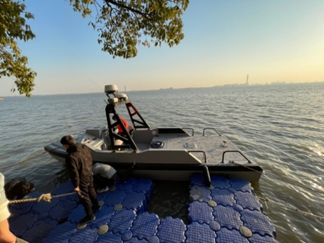
Figure 3: Lake trials for the ’JH7500’ USV

TABLE I: Main Dimensions of The ’JH7500’ USV

Description	Unit	Value
Displacement (m)	$kg$	3000
Length Overall (L)	$m$	7.50
Beam (B)	$m$	2.60
Draft (D)	$m$	0.53
Nozzle Area ($A_{j}$)	$m^{2}$	0.016
Steering Range ($\delta$)	$\degree$	$[-30,30]$

IV-B Approach Setup and Configuration

The hybrid physical-ML model is established using a training set consisting of a maneuver with a random steering angle sequence. The $\nu$-Support Vector Regression ($\nu$-SVR) method is utilized to estimate the parameters for the physical model, as described in [4]. The parameters for the water jet are set as follows: the momentum utilization factor $\alpha$ is 0.95, and the $a$ and $b$ coefficients are 0.0075 and -7.0, respectively. The $X_{\dot{u}}$ for the surge motion is determined using an empirical formula, with a dimensionless value of -0.0072. The identified parameters in dimensionless form are listed in Table. II.

TABLE II: Identified Parameters of The Physical Model

Parameter	Value	Parameter	Value
$X_{u}$	-0.04130	$Y_{0}$	0.00183
$X_{uu}$	0.01600	$R_{r}$	-0.86381
$X_{uuu}$	-0.00022	$R_{\delta}$	0.23587
$Y_{v}$	-0.10667	$R_{rrr}$	-3.09984
$Y_{r}$	-0.00304	$R_{vr\delta}$	-3.33673
$Y_{\delta}$	0.10280	$R_{ur}$	0.12056
$Y_{rrr}$	-4.54642	$R_{r\delta\delta}$	0.07598
$Y_{vr\delta}$	2.15718	$R_{vrr}$	9.66080
$Y_{ur}$	0.00020	$R_{0}$	0.00227

The residual block is trained using a combination of random steering angle sequences and additional data from two turning circle maneuvers. The FNN’s structural parameters are obtained through Bayesian optimization, consisting of two hidden layers with 10 neurons each. The internal weight parameters are optimized using the Adam optimizer with a learning rate of 0.001. The training process involves 800 iterations with a batch size of 64 and the regularization term $\lambda$ of 0.01.

IV-C Comparative Experiments Setup

A comparative test was conducted to assess the performance of the hybrid model in comparison to the physical model and the pure data-driven model. The physical model utilized in the comparison test is the same one used in the hybrid model. The pure data-driven model has a structure similar to the FNN layers in the hybrid model, but its output consists of the accelerations of 3-DOF motions. The pure data-driven model can be expressed as follows:

$$[\hat{\dot{u}},\hat{\dot{v}},\hat{\dot{r}}]^{T}=\mathcal{F}_{DataDriven}(u,v,r,\delta,cos(\psi),sin(\psi)),$$ (15)

where $\hat{\dot{u}}$, $\hat{\dot{v}}$ and $\hat{\dot{r}}$ represent the estimated acceleration for surge, sway, and yaw movements, respectively.

The test set consisted of three turning circle maneuvers and one zigzag-type maneuver, which were not included in the training dataset, to evaluate the model’s generalization performance. It should be noted that the zigzag-type maneuvers conducted during lake trials were not the standard zigzag maneuver test, as the steering angle was not strictly responsive to the heading angle. The three turning tests reflect the vessel’s turning ability, including a 23$\degree$ turning circle test started from the starboard side, a 30$\degree$ turning circle test started from the starboard side, and a 20$\degree$ turning circle test started from the port side. The zigzag-type maneuvering test alternates the rudder angle between -30$\degree$ to 30$\degree$ to assess the vessel’s course-changing ability and yaw checking ability.

The long-term prediction ability of the models is assessed by examining their performance over extended periods. Given the initial motion states and the steering angle sequences, the future motion states and trajectories are iteratively calculated using the model in conjunction with an ODE solver. This process allows for a detailed analysis of how accurately the model can predict the dynamics of the system over time.

IV-D Generalization Validation: Velocity Prediction

The velocity terms predicted by various modeling methods are depicted in Fig. 4 to 7. The baseline is represented by the black line, while the hybrid model, physical model, and pure data-driven model are represented by the red, blue, and orange lines, respectively. It is evident that the actual navigation data of the USV shows periodic oscillations and high-frequency fluctuations due to environmental disturbances, as well as measurement noise.

Figure 4: Velocity predictions of 23° turning circle maneuver (starboard)

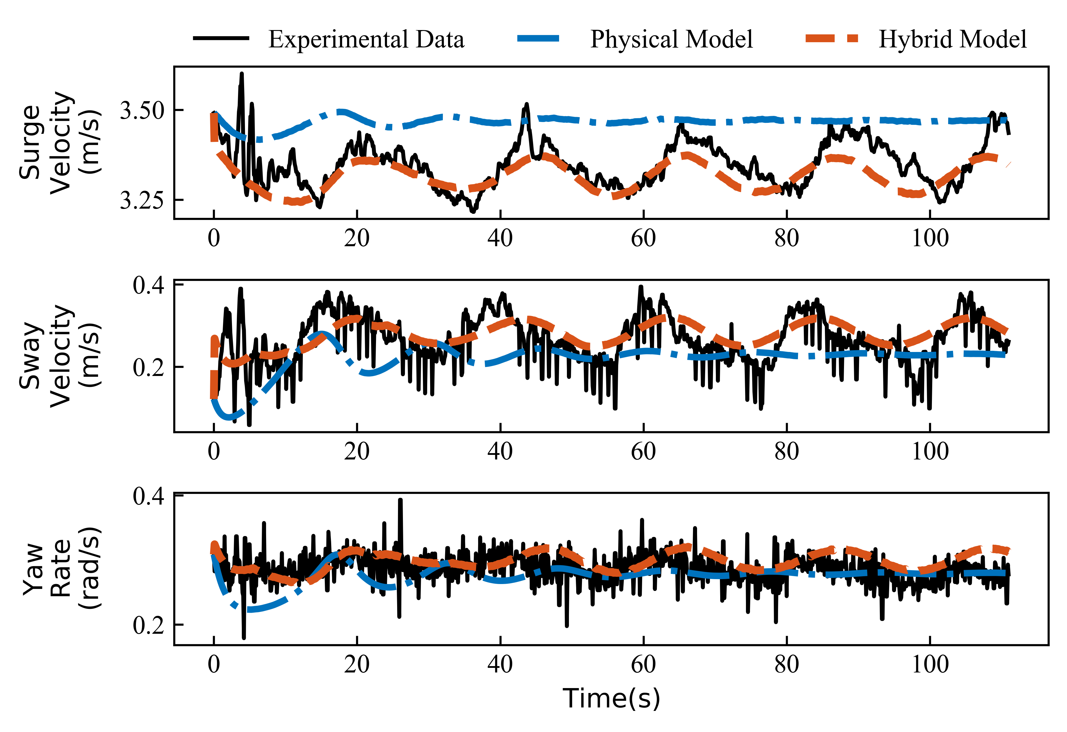
Figure 5: Velocity predictions of 30° turning circle maneuver (starboard)

Figure 6: Velocity predictions of 20° turning circle maneuver (port)]

Figure 7: Velocity predictions of Zigzag-type maneuver

Overall, the hybrid model exhibits greater accuracy and better nonlinear characterization capabilities than both the physical model and the pure data-driven model. In the turning tests, the physical model gradually approaches straight lines, which matches the steady motion of a turning circle maneuver in calm water. However, it fails to capture the periodic oscillations caused by waves and currents, resulting in a discrepancy between the predicted and actual navigation velocities. In contrast, the hybrid model shows higher accuracy in representing the actual navigation velocity, effectively capturing the periodic oscillations of speeds caused by currents and waves.

More specifically, the physical model’s predictions show a deviation from the mean value of the actual surge velocity, with higher predictive values in the 23° and 30° turning tests. This can be attributed to the model’s simplification of only considering the thrust force and the resistance expressed by a polynomial of the surge velocity, while disregarding the influence of other degrees of freedom and control input. Regarding the sway and yaw rate velocities, the discrepancies between the physical model’s predictions and the actual navigation velocities are mainly in the oscillation periods, with smaller numerical differences. On the other hand, the hybrid model incorporates the nonlinear effects by the residual block, on the basis of the physical model. The results show that the predicted values are below those of the physical model for the surge motion, resulting in a better fit for the 23° and 30° turning tests, but a slight deviation in the 20° turning test. In addition, the hybrid model accurately characterizes the periodic oscillations observed in the three DOFs, while disregarding non-periodic high-frequency fluctuations. The zigzag-type test reveals that both the hybrid model and physical model have difficulties in capturing the surge velocity variations accurately, instead yielding an approximate prediction around the average value. In terms of yaw rate, the hybrid model demonstrates greater precision than the physical model.

It should be mentioned that the pure data-driven model exhibits unstable performance in long-term predictions, with high bias or divergence over iterations. Therefore, we only present the results of the 23° and 20° turning tests and do not discuss this model in subsequent contexts.

Table III provides the prediction accuracy of the velocities evaluated by Root Mean Square Error (RMSE). The results align with the analyses presented above, indicating that the hybrid model generally achieves more accurate predictions.

TABLE III: RMSE of Velocity Predictions Across Different Models

		23° turning circle maneuver	30° turning circle maneuver	20° turning circle maneuver	Zigzag-type maneuver
	Surge velocity	0.1322	0.1432	0.0540	0.1188
Physical Model	Sway velocity	0.0700	0.0788	0.0749	0.0435
	Yaw rate	0.0325	0.0286	0.0206	0.0538
	Surge velocity	0.0513	0.0575	0.0907	0.1172
Hybrid Model	Sway velocity	0.0459	0.0509	0.0479	0.0462
	Yaw rate	0.0254	0.0268	0.0217	0.0232

IV-E Generalization Validation: Trajectory Prediction

Fig. 8 and 9 show the predicted trajectories for both the hybrid model and the physical model. As can be seen, the physical model can captures the motion trend of the USV in both the turning and zigzag-type tests. However, there is a noticeable drift between the predicted trajectories and the experimental results. This discrepancy could be attributed to the accumulation of velocity biases during iterations, which leads to a more significant bias in trajectory predictions. In contrast, the hybrid model effectively addresses this issue and generates trajectories that closely align with the overall trajectory.

Figure 8: Trajectory predictions of 30° turning circle maneuver (port)

Figure 9: Trajectory predictions of zigzag-type maneuver

To evaluate how well each model captures the main dynamic features related to navigation safety and turning capability, the turning diameters from both models are compared against the actual turning diameters, as presented in Table. IV. Both the physical model and hybrid model demonstrate sufficient accuracy, with the maximum error being less than 9%. This indicates that although the physical model is imperfect, it still captures the fundamental characteristics of the USV. In comparison, the hybrid model exhibits a notably improved performance, with a significant reduction in prediction error compared to the physical model for the 30° turning test.

TABLE IV: Model Performance in Turning Diameter Predictions

Maneuvers	Actual value/(m)	Physical Model/(m)	Relative Error/(%)	Hybrid Model/(m)	Relative Error/(%)
23° turning circle maneuver	26.50	29.61	11.74	29.29	10.53
30° turning circle maneuver	22.18	24.85	12.04	22.51	1.49
20° turning circle maneuver	32.93	34.94	6.10	34.24	3.98

IV-F Analytical Discussion

In summary, the hybrid physics-ML model demonstrates great capabilities in long-term motion prediction in specific environmental conditions. The study case results demonstrate that the hybrid model architecture has a balancing effect on modeling stability and expressive capability. In the hybrid physical-ML model, the simplified physical model reduces the effort needed to construct precise hydrodynamic force/moment formulations while still reflecting certain fundamental dynamic characteristics and providing interpretability. Additionally, the data-driven module offers the capability for nonlinear mapping, enhancing the model’s representation of nonlinear dynamics. Constrained by the physical mechanism model, the hybrid modeling approach exhibits good robustness with a limited amount of data. Even when the data is filled with environmental disturbances and measurement noise, it remains stable and builds a model with good generalizability.

It is worth mentioning that this paper also highlights the usefulness of the trigonometric transformation of the heading angle as an additional feature to extract the periodic effects. This transformation enable the modeling of information related to the influence of waves and currents, which is difficult to formulate or measure in real-world scenarios. In this way, even without environmental sensors, the model can account for disturbances caused by environmental factors. However, it is important to note that such hybrid models are restricted to the specific environmental conditions associated with the training data. This can be seen as a limitation of the current version of the hybrid modeling framework. If conditions permit, further integration of environmental sensor information into additional feature variables could significantly enhance the adaptability of the model.

V Conclusions

This paper presents a hybrid physical-ML framework designed to characterize the dynamic properties of surface vehicles under environmental disturbances. The effectiveness of the method has been validated using experimental data obtained from the 7.5-meter USV. By incorporating an imperfect physical model into a residual block of FNN, this approach combines the constrained nature of mechanistic modeling with the nonlinear mapping capability of data-driven modeling, demonstrating interpretability, generalizability, and robustness. These results highlight the potential of integrating mechanistic knowledge with machine learning for nonlinear dynamic modeling.

For the specific problem, this study focuses on maneuver-level motion modeling of a surface vehicle, which is relatively microscale perspective compared to studies of long-term voyages for large vessels. The results exhibit good long-term predictive capabilities for maneuvers such as turning and zigzag-type maneuvers under environmental disturbances. These outcomes are crucial for the development of high-fidelity simulators and intelligent decision-making and control systems.

References

- [1] M. A. Abkowitz, “Lectures on ship hydrodynamics–steering and manoeuvrability,” Tech. Rep., 1964.
- [2] A. Ogawa and H. Kasai, “On the mathematical model of manoeuvring motion of ships,” International shipbuilding progress, vol. 25, no. 292, pp. 306–319, 1978.
- [3] H. K. Yoon and K. P. Rhee., “Identification of hydrodynamic coefficients in ship maneuvering equations of motion by estimation-before-modeling technique,” Ocean Engineering, vol. 30, pp. 2379–2404, 2003.
- [4] Z. Wang, Z. Zou, and C. G. Soares, “Identification of ship manoeuvring motion based on nu-support vector machine,” Ocean Engineering, vol. 183, pp. 270–281, 2019.
- [5] Y. Xue, Y. Liu, C. Ji, and G. Xue, “Hydrodynamic parameter identification for ship manoeuvring mathematical models using a bayesian approach,” Ocean Engineering, vol. 195, p. 106612, 2020.
- [6] N. Wang, M. J. Er, and M. Han, “Dynamic tanker steering control using generalized ellipsoidal-basis-function-based fuzzy neural networks,” IEEE Transactions on Fuzzy Systems, vol. 23, no. 5, pp. 1414–1427, 2014.
- [7] Y. L. H. Shen, G. Wen and J. Zhou, “A stochastic event-triggered robust unscented kalman filter-based usv parameter estimation,” IEEE Transactions on Industrial Electronics, vol. 71, no. 9, pp. 11 272–11 282, 2024.
- [8] D. Moreno-Salinas, R. Moreno, A. Pereira, J. Aranda, and J. M. de la Cruz, “Modelling of a surface marine vehicle with kernel ridge regression confidence machine,” Applied Soft Computing, vol. 76, pp. 237–250, 2019.
- [9] Z. Wang, H. Xu, L. Xia, Z. Zou, and C. G. Soares, “Kernel-based support vector regression for nonparametric modeling of ship maneuvering motion,” Ocean Engineering, vol. 216, p. 107994, 2020.
- [10] W. A. Ramirez, Z. Q. Leong, H. Nguyen, and S. G. Jayasinghe, “Non-parametric dynamic system identification of ships using multi-output gaussian processes,” Ocean Engineering, vol. 116, pp. 26–36, 2018.
- [11] H. W. He, Z. H. Wang, Z. J. Zou, and Y. Liu, “Nonparametric modeling of ship maneuvering motion based on self-designed fully connected neural network,” Ocean Engineering, vol. 251, p. 111113, 2022.
- [12] C.-Z. Chen, S.-Y. Liu, Z.-J. Zou, L. Zou, and J.-Z. Liu, “Time series prediction of ship maneuvering motion based on dynamic mode decomposition,” Ocean Engineering, vol. 286, p. 115446, 2023.
- [13] L. Hao, Y. Han, C. Shi, and Z. Pan, “Recurrent neural networks for nonparametric modeling of ship maneuvering motion,” International Journal of Naval Architecture and Ocean Engineering, vol. 14, p. 100436, 2022.
- [14] Y. Jiang, X.-R. Hou, X.-G. Wang, Z.-H. Wang, Z.-L. Yang, and Z.-J. Zou, “Identification modeling and prediction of ship maneuvering motion based on lstm deep neural network,” Journal of Marine Science and Technology, vol. 27, no. 1, pp. 125–137, 2022.
- [15] T. Zhang, X.-Q. Zheng, and M.-X. Liu, “Multiscale attention-based lstm for ship motion prediction,” Ocean Engineering, vol. 230, p. 109066, 2021.
- [16] L. Dong, H. Wang, and J. Lou, “An attention mechanism model based on positional encoding for the prediction of ship maneuvering motion in real sea state,” Journal of Marine Science and Technology, pp. 1–17, 2024.
- [17] Z. Wang, J. Kim, and N. Im, “Non-parameterized ship maneuvering model of deep neural networks based on real voyage data-driven,” Ocean Engineering, vol. 284, p. 115162, 2023.
- [18] J. Jang, C. Lee, and J. Kim, “A learning-based approach to surface vehicle dynamics modeling for robust multistep prediction,” Autonomous Robots, vol. 47, no. 6, pp. 797–808, 2023.
- [19] T. Wang, R. Skulstad, M. Kanazawa, G. Li, and H. Zhang, “Learning nonlinear dynamics of ocean surface vessel with multistep constraints,” IEEE Transactions on Industrial Informatics, 2024.
- [20] J. Lou, H. Wang, J. Wang, Q. Cai, and H. Yi, “Deep learning method for 3-dof motion prediction of unmanned surface vehicles based on real sea maneuverability test,” Ocean Engineering, vol. 250, p. 111015, 2022.
- [21] J. Willard, X. Jia, S. Xu, M. Steinbach, and V. Kumar, “Integrating scientific knowledge with machine learning for engineering and environmental systems,” pp. 1–37, 2022.
- [22] R. Skulstad, G. Li, T. I. Fossen, B. Vik, and H. Zhang, “A hybrid approach to motion prediction for ship docking—integration of a neural network model into the ship dynamic model,” IEEE Transactions on Instrumentation and Measurement, vol. 70, pp. 1–11, 2020.
- [23] M. Kanazawa, T. Wang, R. Skulstad, G. Li, and H. Zhang, “Knowledge and data in cooperative modeling: Case studies on ship trajectory prediction,” Ocean Engineering, vol. 266, p. 112998, 2022.
- [24] M. Kanazawa, R. Skulstad, T. Wang, G. Li, L. I. Hatledal, and H. Zhang, “A physics-data co-operative ship dynamic model for a docking operation,” IEEE Sensors Journal, vol. 22, no. 11, pp. 11 173–11 183, 2022.
- [25] Y. Han, L. Hao, C. Shi, Z. Pan, and G. Min, “Prediction of ship maneuvering motion with grey-box modelling incorporating mechanism and data,” Ships and Offshore Structures, pp. 1–14, 2023.
- [26] T. Wang, G. Li, L. I. Hatledal, R. Skulstad, V. Æsøy, and H. Zhang, “Incorporating approximate dynamics into data-driven calibrator: A representative model for ship maneuvering prediction,” IEEE Transactions on Industrial Informatics, vol. 18, no. 3, pp. 1781–1789, 2021.
- [27] R. E. Nielsen, D. Papageorgiou, L. Nalpantidis, B. T. Jensen, and M. Blanke, “Machine learning enhancement of manoeuvring prediction for ship digital twin using full-scale recordings,” Ocean Engineering, vol. 257, p. 111579, 2022.
- [28] K. He, X. Zhang, S. Ren, and J. Sun, “Deep residual learning for image recognition,” in Proceedings of the IEEE Conference on Computer Vision and Pattern Recognition, 2016, pp. 770–778.