The transfer of Bell nonlocality between two and three-qubit dissipative systems with counter-rotating-wave terms

Abstract

We investigate the effect of counter-rotating-wave terms on bell nonlocality (BN) and entanglement for three qubits coupled with a Lorentz-broadened cavity mode at zero temperature for strong and ultrastrong coupling regimes by employing exact numerical hierarchical equations of motion approach (HEOM). Our findings are as follows: (i) the counter-rotating wave terms significantly increase the rate of decoherence in the three-qubit system; (ii) a consistent transfer of Bell nonlocality between the three-qubit state and its subsystem is observed when the interaction between the qubits and the bath is asymmetrical, which provides effective numerical evidence for the monogamy and complementarity of multipartite nonlocality; (iii) the counter-rotating wave terms can enhance genuine tripartite nonlocality in the qubit system; and (iv) these terms do not significantly generate three-party correlations in zero-excitation cases, which differs from previous studies involving two qubits.

I Introduction

Bell nonlocality (BN), as the fundamental concept of quantum mechanics, allows the tensorial non-separable bipartite states to correlate with each other even in the space-like interval, which can arise from quantum entanglement [1, 2, 3]. In previous studies, quantum entanglement and BN for two parties have been extensively studied experimentally [4, 5, 6, 7, 8] and theoretically [9, 10, 11, 12], demonstrating their advantages over classical physics. However, the quantification of multipartite entanglement and nonlocality becomes much more complicated [13]. To address this, a new important concept referred to as “genuine” has been introduced for multipartite systems [14], which includes genuine tripartite entanglement (GTE) [15, 16, 17] and nonlocality (GTN) [18]. As experiments progress, results indicate that both the maximum entangled three-qubit W [19] state and the GHZ state [20] exhibit GTN and GTE correlations, revealing that these correlations have benefits for processing quantum information tasks [21, 22, 23, 24]. For example, GTN demonstrates a unique application value since it can work against a conspiring (cheating) sub-group of parties in applying quantum communication complexity [25, 26], and GTE is crucial for quantum algorithms to achieve an exponential speed-up over classical computation [27, 28].

However, GTN and GTE may be destroyed rapidly due to the unavoidable coupling between the microcosmic quantum system and its surrounding environment, which is the main challenge in quantum information processing [29]. The study of quantum open system dynamics has gained significant attention in recent decades due to its potential to simulate various physical processes [30]. Traditionally, the dynamics of most exactly solvable open quantum system models involve various approximations, such as Born-Markovian, perturbative, and rotating wave approximations (RWA) [31, 32]. These approximations are valid when the coupling between the system and the environment is weak and the time scale of the environment is significantly shorter than that of the system [29]. Unfortunately, the above approximations do not accurately predict real physical processes in the strong coupling regime because they fail to describe the dynamics of the environment completely [33, 34, 35]. For example, many studies have examined the dynamics of two- or three-qubit quantum correlations in non-Markovian environments with significant memory effects [36, 37, 38]. In these cases, the correlation in the quantum system may revive due to the information flowing back from the environment, which is a typical characteristic of a non-Markovian quantum process. However, the dynamics of those studies are based on the RWA, which neglects the counter-rotating-wave terms; other studies that include the effects of counter-rotating wave terms rely on perturbative approximations [39, 40, 41], which are not applicable in cases of strong coupling regime. Naturally, we have an interesting question: What effects do the counter-rotating wave terms have on entanglement and BN of three-qubit systems in a strong coupling regime without the approximations above? Here, we investigate the time evolution of three-qubit systems interacting with a common bath using numerical hierarchical equations of motion (HEOM) [42, 43, 44]. The HEOM is a precise method to describe the non-Markovian dynamics of a system interacting with one or more baths at finite temperatures without the approximations above, which is widely applied in the study of quantum dissipative systems [33, 34, 35, 45, 46, 47].

In this paper, we utilize the HEOM scheme to investigate a model consisting of three noninteracting qubits that couple to a common bosonic bath. This model has been solved precisely for two qubits under the RWA [38]. Here, we extend the analysis from the two-qubit case to the three-qubit scenario and obtain an exact solution. By comparing the results with and without the RWA, we analyze the impact of the counter-rotating wave terms on the dynamic evolution of the entanglement and BN of the reduced three-qubit system. In the strong coupling regime, we observe that the counter-rotating wave terms notably enhance the decoherence rate of the reduced qubit system and diminish the sudden birth strength of GTE and GTN that arises from the memory effect of the bath. However, we find that the counter-rotating wave terms can enhance the sudden birth of GTN but do not have the same effect on GTE for the ultrastrong coupling regime. In addition, we examine the mechanisms involved in the creation and destruction of quantum resources. Specifically, we observed the continuous transfer of Bell nonlocality between the three-qubit system and its subsystem by varying the coupling strength between the qubits and the bath, which is a novel phenomenon. We also consider the scenario in which the initial state has no excitations. Our results show that the counter-rotating wave terms are ineffective in inducing GTE and GTN for the entire qubit system. However, entanglement can still be generated within two-qubit subsystems, which indicates that the virtual excitations created by the counter-rotating wave terms are insufficient to produce a genuine three-party correlation.

This paper is organized as follows. In Sec. II, we first introduce the methods used in this paper to quantify the entanglement and nonlocality in two-qubit and three-qubit systems. Next, we introduce the model studied in this paper and outline the steps for obtaining the time evolution under the non-RWA and RWA approaches. In Sec. III, we investigate the influence of the counter-rotating-wave terms on the entanglement and BN in both strong and ultrastrong coupling regimes. The main conclusions of this paper are presented in Sec. IV. In the Appendix. A and B, we outline the steps for using the HEOM method to obtain the dynamics of the reduced qubit system without applying the RWA and provide the exact dynamic equation when the RWA is applied.

II Preliminaries

II.1 Entanglement and Bell nonlocality

For a two-qubit system represented by the density matrix $\rho_{ab}$, there are several schemes for measuring the entanglement between qubits $a$ and $b$, including negativity [48], discord [49], and concurrence [50]. In this paper, we use concurrence to measure entanglement because it is a simple but reliable method widely employed in relevant research. In quantum correlation, entanglement is considered a more fundamental type of correlation because it serves as the source of BN. While BN arises from entanglement, it is important to note that entanglement does not necessarily imply BN [3, 51]. To assess whether a two-qubit system exhibits the nonlocal correlation, we can apply the CHSH inequality [52]. The local correlated two-qubit state $\rho_{ab}$ must satisfy the CHSH inequality, which can be expressed as

$$\operatorname{tr}(\rho_{ab}S)\leq 2,$$ (1)

where $S$ is the CHSH operator, and the inequality can be calculated for any two-qubit density matrix using the following expression [9]:

$$\mathcal{N}(\rho_{ab}) =\max_{S}\operatorname{tr}(\rho_{ab}S),$$

$$=2\sqrt{\lambda_{1}+\lambda_{2}},$$ (2)

where $\mathcal{N}(\rho_{ab})$ denotes the maximal value of the CHSH expression for a arbitrary two-qubit state $\rho_{ab}$. if $\mathcal{N}(\rho_{ab})>2$, the two-qubit state must be nonlocal. Besides, $\lambda_{1}$ and $\lambda_{2}$ are the spectral decomposition of the matrix $T^{T}T=\sum_{k=1}^{3}\lambda_{k}\left|\mu_{k}\right\rangle\left\langle\mu_{k}\right|$ in nonincreasing order. The $3\times 3$ matrix $T$ is constructed using the Pauli operators given by the vector $\vec{\sigma}=(\sigma_{1},\sigma_{2},\sigma_{3})$, where the entries of the matrix are defined as $T_{jk}=\operatorname{tr}(\sigma_{j}\otimes\sigma_{k}\rho)$.

However, the definition of entanglement is significantly different when we consider entanglement beyond the two-qubits system. In recent decades, many GTE measures have been proposed [15, 16, 17, 14, 53, 54], but only a few ways to effectively calculate the GTE for general three-qubit states, primarily due to the challenges involved in identifying the optimal decompositions of mixed three-qubit states. Thus, we choose the method of $\pi$-tangle to quantify the GTE since this method provides an explicit analytical expression for arbitrary three-qubit states and can be defined in the following manner [55, 56]:

$$\pi_{abc}=\frac{1}{3}\left(\pi_{a}+\pi_{b}+\pi_{c}\right),$$ (3)

where, $\pi$-tangle is the average of $\pi_{a}$, $\pi_{b}$ and $\pi_{c}$.

$$\begin{array}[]{l}\pi_{a}=N_{a(bc)}^{2}-N_{ab}^{2}-N_{ac}^{2},\\ \pi_{b}=N_{b(ac)}^{2}-N_{ba}^{2}-N_{bc}^{2},\\ \pi_{c}=N_{c(ab)}^{2}-N_{ca}^{2}-N_{cb}^{2},\end{array}$$ (4)

where $N_{a(bc)}=\|\rho_{abc}^{T_{a}}\|-1$ and $N_{ab}=\|\rho_{ab}^{T_{a}}\|-1$ are the negativity for a two- and three-qubit state, respectively. $T_{a}$ denotes the partial transpose of $\rho_{abc}$ or $\rho_{ab}$, and $\|M\|$ is the trace norm for a matrix M. The other symbols have the same definition like $N_{a(bc)}$ and $N_{ab}$.

As for GTN, it can be quantified by using the Svetlichny inequality [18]

$$\operatorname{tr}(S\rho_{abc})\leq 4,$$ (5)

where the maximal value violating the Svetlichny inequality of the tripartite state $\rho_{abc}$ can be denoted as

$$\mathcal{N}(\rho_{abc})\equiv\max_{S}\operatorname{tr}(S\rho_{abc}).$$ (6)

If $\mathcal{N}(\rho_{abc})>4$, then the three-qubit system must exhibit GTN. However, there is no specific analytic expression to calculate $\mathcal{N}(\rho_{abc})$ for generalized three-qubit state due to computational complexity since here we use the “exact” numerical method to quantify the three-qubit states whether violating the Svetlichny inequality [57].

II.2 The Model

In this subsection, we derive the dynamics of the reduced density matrix for three non-interacting qubits in a common bath, considering both cases with and without RWA. The Hamiltonian of the total system without RWA can be described by

$$\hat{H}=\omega_{0}\sum_{i=1}^{3}\left(\hat{\sigma}_{+}^{(i)}\hat{\sigma}_{-}^{(i)}\right)+\sum_{k}\omega_{k}\hat{a}_{k}^{\dagger}\hat{a}_{k}+\hat{V}\otimes\sum_{k}g_{k}\left(\hat{a}_{k}^{\dagger}+\hat{a}_{k}\right),$$ (7)

where $\hat{\sigma}_{\pm}^{(j)}$ is the spin-flip operators, $\omega_{0}$ and $\omega_{k}$ denote the frequencies of qubit and bath, $\hat{a}_{k}^{\dagger}$ and $\hat{a}_{k}$ are the creation and annihilation operators of the bath. Besides, $\hat{V}=\sum_{i=1}^{3}\alpha_{i}\hat{\sigma}_{x}^{i}$ denotes the qubits system coupled to the bath, containing the counter-rotating-wave terms. The coupling strength of the $i$th qubit with the bath is denoted by $\alpha_{i}$.

In this paper, we examine the structured bath as the electromagnetic field within a lossy cavity, where the qubit-cavity coupling spectrum takes on a Lorentzian form due to the broadening of the fundamental mode [38]

$$J(\omega)=\frac{1}{\pi}\frac{\lambda\gamma}{\left(\omega-\omega_{0}\right)^{2}+\gamma^{2}},$$ (8)

here $\lambda$ is proportional to the vacuum Rabi frequency and can approximately interpreted as the system-bath coupling strength, $\gamma$ is the width of the distribution and the quantity $\frac{1}{\gamma}$ is the lifetime of the mode. Besides, the ratio $R=\frac{\alpha_{t}\sqrt{\lambda}}{\gamma}$ denotes the boundary between Markovian regimes and non-Markovian regimes,where $\alpha_{t}$ is the collective coupling strength defined in Appendix. B. When $R\gg 1$, it indicates that the qubits and the bath are strongly coupled, which implies that the memory effects of the bath must be considered, and the dynamics of this open system are non-Markovian. The evolution of the reduced qubit system in the model we discussed can be analyzed using the HEOM method, with additional details provided in Appendix. A.

In the following, we will provide the exact solution to the above model under the RWA. Suppose the initial state of the system is

$$|\psi(0)\rangle=\ket{W}\otimes|0\rangle_{R},$$ (9)

where $\ket{W}=\frac{1}{\sqrt{3}}[\ket{egg}+\ket{geg}+\ket{gge}]$ and the time evolution is described by

$$|\psi(t)\rangle =c_{1}(t)|e,g,g\rangle|\mathbf{0}\rangle_{R}+c_{2}(t)|g,e,g\rangle|\mathbf{0}\rangle_{R}$$

$$+c_{3}(t)|g,g,e\rangle|\mathbf{0}\rangle_{R}+\sum_{k}c_{k}(t)|g,g,g\rangle\left|1_{k}\right\rangle_{R},$$ (10)

where $\left|1_{k}\right\rangle_{R}$ denotes the one excitation state in the $k$th mode. By tracing over the bath degrees of freedom, the reduced three-qubit density matrix $\rho_{abc}$ takes the form

$$\rho_{abc}=\left(\begin{array}[]{cccccccc}0&0&0&0&0&0&0&0\\ 0&0&0&0&0&0&0&0\\ 0&0&0&0&0&0&0&0\\ 0&0&0&\left|c_{1}\right|^{2}&0&c_{1}c^{*}_{2}&c_{1}c^{*}_{3}&0\\ 0&0&0&0&0&0&0&0\\ 0&0&0&c_{2}c^{*}_{1}&0&\left|c_{2}\right|^{2}&c_{2}c_{3}^{*}&0\\ 0&0&0&c_{3}c^{*}_{1}&0&c_{3}c^{*}_{2}&\left|c_{3}\right|^{2}&0\\ 0&0&0&0&0&0&0&\left|c_{k}\right|^{2}\end{array}\right).$$ (11)

Then, following procedures shown Appendix. B, the amplitudes $c_{i}$ are obtained

$$c_{1}(t) =\left[r_{2}^{2}+r_{3}^{2}+r_{1}^{2}\mathcal{E}(t)\right]c_{1}(0)-r_{1}r_{2}[1-\mathcal{E}(t)]c_{2}(0)$$ (12)

$$-r_{1}r_{3}[1-\mathcal{E}(t)]c_{3}(0),$$

$$c_{2}(t) =\left[r_{1}^{2}+r^{2}_{3}+r_{2}^{2}\mathcal{E}(t)\right]c_{2}(0)-r_{1}r_{2}[1-\mathcal{E}(t)]c_{1}(0)$$

$$-r_{2}r_{3}[1-\mathcal{E}(t)]c_{3}(0),$$

$$c_{3}(t) =\left[r_{1}^{2}+r_{2}^{2}+r_{3}^{2}\mathcal{E}(t)\right]c_{3}(0)-r_{1}r_{3}[1-\mathcal{E}(t)]c_{1}(0)$$

$$-r_{2}r_{3}[1-\mathcal{E}(t)]c_{2}(0).$$

III Results

In this section, we investigate the evolution of entanglement and BN in two- and three-qubit systems for strong and ultrastrong coupling regimes, beginning with the initial W state. There are two primary reasons for choosing the W state as the initial three-qubit state. Firstly, previous studies have demonstrated that the W and GHZ states have GTN and GTE both experimentally [21, 24] and theoretically [19, 20]. However, most studies [58, 51, 59, 60] have only been able to analyze the GTN of general GHZ-like states using an exact expression for $\mathcal{N}(\rho_{abc})$. Due to theoretical computational challenges, there are currently no specific analytical expressions available to calculate $\mathcal{N}(\rho_{abc})$ for general W states. Thus, it is valuable to investigate how the GTN of W states evolves in real environments (dissipative systems) and understand whether there is a phenomenon of “sudden death” or “sudden birth”  [61] of GTN during the evolution in this context deserves further exploration. Secondly, in the model we considered, when the coupling strength of all qubits to the bath is uniform (e.g., $\alpha_{1}=\alpha_{2}=\alpha_{3}$), the probability amplitude $c_{j}(t)$ evolution remains consistent due to the symmetry of the W state. However, what interesting physical phenomena can arise from inconsistent system-environment interactions due to varying coupling strengths? Here, we provide clear answers to the questions.

III.1 The cases of strong coupling regime

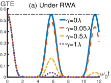
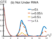
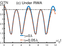
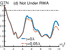
Figure 1: (a) GTE of the three-qubit system obtained by the exactly analytic expression with RWA for various values of $\gamma$; other parameters are chosen as $\alpha_{1}=\alpha_{2}=\alpha_{3}=1$, $\lambda=0.1\omega_{0}$, $\omega_{0}=1$ and the initial state is $\psi(0)=\ket{W}\otimes|0\rangle_{R}$. (b) The same as (a), but GTE obtained by the numerical HEOM method without RWA. (c) The same as (a), but GTN is quantified by calculating maximal violating of the Svetlichny inequality $\mathcal{N}(\rho_{abc})$, and no sudden birth of GTN is detected for the cases where $\gamma=0.5\lambda$ and $\gamma=1\lambda$. (d) The same as (c), but RWA is not applied here, and there is no sudden birth of GTN for all parameters $\gamma$.

In this subsection, we focus on the strong coupling regime ($\lambda=0.1\omega_{0}$) and compare the results obtained by the above methods for the initial W state. In Fig. 1, we present the GTE and GTN for the reduced three-qubit system. These results are obtained using the numerical HEOM method without RWA, as well as the exact analytic expression that applies RWA, detailed in Eq. (11). A comparison of Fig. 1(a) and Fig. 1(b) shows that the counter-rotating wave terms significantly accelerate the decoherence of GTE and suppress its sudden births. In Fig. 1(a), the GTE (blue solid line) displays a trend of periodic evolution that does not decay with $\gamma=0$. This behavior occurs because the mode’s lifetime $\tau_{c}=\frac{1}{\gamma}$ is infinite in the single-mode limit. In contrast, GTE clearly diminishes when RWA is not applied, as shown by the blue solid line in Fig. 1(b). As for GTN, we can find that the reduced three-qubit system violates the Svetlichny inequality with $\mathcal{N}(\rho_{abc})>4$ at the beginning, and the phenomenon of sudden death and sudden birth of GTN can be found due the memory effect of the bath in Fig. 1(c). However, in Fig. 1(d), the Svetlichny inequality is not violated in any cases except for the initial time interval. Consequently, the results indicate that the RWA enhances the strength of GTN and GTE due to the contribution of the counter-rotating wave terms that are neglected in quantum simulations, which fails to describe real physics.

Next, we study the significant phenomenon caused by inconsistent coupling strengths ($\alpha_{1}=\alpha_{2}\neq\alpha_{3}$) between the qubits and bath.

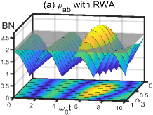
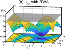
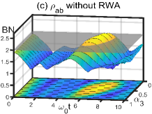
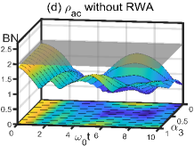
Figure 2: The BN is quantified by calculating maximal violating of the CHSH inequality for the subsystem $\mathcal{N}(\rho_{ab})$ and $\mathcal{N}(\rho_{ac})$, which is analyzed using both the exact analytic expression with RWA and the numerical HEOM method without RWA for different parameters: the coupling strength between the third qubit and the bath, denoted as $\alpha_{3}$, varies from 0 to 1; other parameters are set as $\alpha_{1}=\alpha_{2}=1$, $\lambda=0.1\omega_{0}$, $\omega_{0}=1$ and the initial state is $\psi(0)=\ket{W}\otimes|0\rangle_{R}$. Due to the symmetry, we have $\rho_{ac}(t)=\rho_{bc}(t)$. In addition, the sudden birth of GTN is not observed in all cases.

In Fig. 2 (a) and (c), it is evident that the CHSH inequality is violated for the subsystem $\rho_{ab}$ when $\alpha_{3}\neq\alpha_{i}$ (i=1,2), both with and without the RWA. The results also show that stronger BN is observed when the RWA is applied. However, there is no violation of the CHSH inequality for the subsystem $\rho_{ac}$ and $\rho_{bc}$ throughout the time evolution. This observation is intriguing because it suggests that subsystems can exhibit nonlocal correlations due to the asymmetrical coupling between the qubits and the bath. Moreover, the counter-rotating wave terms seem to reduce BN. Furthermore, although the three-qubit system initially exhibits GTN, there is no sudden birth of GTN during the subsequent time evolution, and nonlocality is transferred from the three-qubit system to its subsystems. The results above raise two critical questions: $(i)$. Why does the asymmetric coupling between qubits and the bath result in BN? $(ii)$. Why is the violation of the CHSH inequality more pronounced under the RWA?

To explore these questions, we systematically investigate the entanglement in two- and three-qubit systems from the perspective of information flows. In Fig. 3, it can be observed that GTE and concurrence of the qubit systems decay rapidly to zero in both cases as the information from the qubit systems flows into the bath. However, the amount of information flowing back to the three qubits varies due to differences in coupling strength. This variation results in differing amplitude of concurrence revival for the states $\rho_{ab}$ and $\rho_{ac}$. More specifically, when comparing Fig. 3 (b) and (c), it is evident that the revival of the concurrence for subsystem $\rho_{ab}$ caused by the bath’s information flowing back (or memory effect) is significantly greater than that of subsystem $\rho_{ac}$ when the coupling strength $\alpha_{3}$ is around 0.5. This phenomenon occurs because when the information flows from the bath returns to the qubit system, more information is transferred back to subsystem $\rho_{ab}$, since the coupling strength $\alpha_{1}=\alpha_{2}\textgreater\alpha_{3}$. In the following, we focus on the power of counter-rotating-wave terms during the time evolution of the state $\rho_{abc}(t)$ and $\rho_{ab}(t)$. In previous research [33], the results show that the counter-rotating-wave terms can obviously enhance the memory effect in the boson environment compared with the cases of RWA. However, our result shows that the revival amplitude of GTE and concurrence is significantly reduced under the non-RWA in Fig. 3 (d)-(f), which shows the counter-rotating-wave terms weakens the memory effect, resulting in more information being dissipated in the bath.

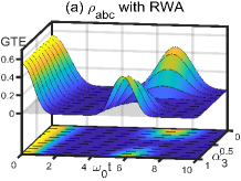
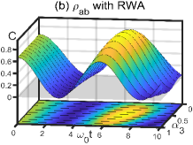
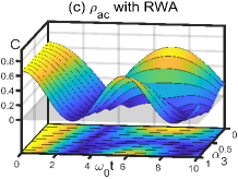
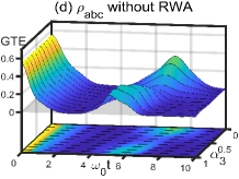
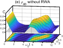
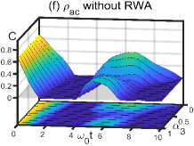
Figure 3: The dynamics of GTE and concurrence for the reduced three-qubit system $\rho_{abc}(t)$ and two-qubit subsystems $\rho_{ab}(t)$ and $\rho_{ac}(t)$, both with and without the RWA, are plotted as the function of $\omega_{0}t$ for different parameters: $\alpha_{3}$ varies from 0 to 1; other parameters are set as $\alpha_{1}=\alpha_{2}=1$, $\lambda=0.1\omega_{0}$, $\omega_{0}=1$ and the initial state is $\psi(0)=\ket{W}\otimes|0\rangle_{R}$. Besides, the sudden birth of GTN is not detected by using Svetlichny inequality throughout the time evolution of $\rho_{abc}(t)$ for all cases.

III.2 The cases of ultrastrong coupling regime

In this subsection, we study the impact of the counter-rotating wave terms on the qubit system when its coupling strength is ultrastrong with the bath.

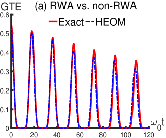
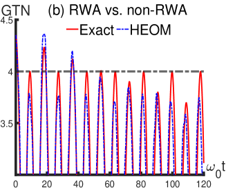
Figure 4: (a) GTE of the three-qubit system is obtained using the numerical HEOM method without the RWA and the exact analytic expression with the RWA for ultrastrong coupling regime $\lambda=0.01\omega_{0}$. The parameters are set as follows: $\gamma=0.01\lambda$, $\omega_{0}=1$, and $\alpha_{1}=\alpha_{2}=\alpha_{3}=1$. The initial state is defined as $|\psi(0)\rangle=\ket{W}\otimes|0\rangle_{R}$. (b) the same as (a), but here the GTN is calculated by calculating maximal violating of the Svetlichny inequality $\mathcal{N}(\rho_{abc})$. Besides, there is no sudden birth of BN for any subsystem.

In Fig. 4(a), one can find that GTE can effectively revive the effect of memory effect in both RWA and non-RWA cases, and the counter-rotating-wave terms weaken the revival amplitude of GTE, which shows that the dynamic evolution is quite different compared with strong coupling cases. In Fig. 4(b), the GTN also shows a series of sudden deaths and births phenomenon. However, the counter-rotating wave terms significantly enhance the strength of the GTN, suggesting that the virtual excitations caused by these counter-rotating wave terms play very different roles in different quantum correlations.

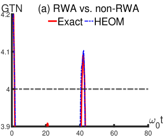
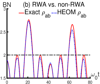
Figure 5: (a) GTN of the three-qubit system is obtained by calculating maximal violating of the Svetlichny inequality $\mathcal{N}(\rho_{abc})$ with and without the RWA. The parameters are set as follows: $\gamma=0.01\lambda$, $\omega_{0}=1$, $\alpha_{1}=\alpha_{2}=1$ and $\alpha_{3}=0.5$. The initial state is defined as $|\psi(0)\rangle=\ket{W}\otimes|0\rangle_{R}$. (b) the same as (a), but here the maximal violating of the CHSH inequality $\mathcal{N}(\rho_{ab})$ is calculated for subsystem $\rho_{ab}$. Due to symmetry, we have $\rho_{ac}(t)=\rho_{bc}(t)$. The BN is not observed for subsystems $\rho_{ac}(t)$ and $\rho_{bc}(t)$ throughout the time evolution.

In the preceding subsection, we discussed the phenomenon of BN transfer from the three-qubit system $\rho_{abc}$ to its subsystem $\rho_{ab}$ in Fig. 2. It is important to note that the sudden birth of GTN is not observed in these cases. However, when we focus on the ultrastrong coupling regime, we can see the transfer of nonlocality back and forth in both the three-qubit and two-qubit systems. In Fig. 5 (a) and (b), both the Svetlichny inequality and the CHSH inequality are violated at different time intervals. Specifically, the three-qubit system demonstrates GTN while the subsystem is local at $\omega_{0}t=0$. The CHSH inequality is violated around $\omega_{0}t=20$, and GTN disappears simultaneously. This suggests that nonlocality has transitioned from the three-qubit system to the subsystem $\rho_{ab}$ due to the interaction between the qubit system and bath. Moreover, the Svetlichny inequality is violated around $\omega_{0}t=40$, without detectable two-body BN, which indicates a transfer of nonlocality from the subsystem back to the overall system. Finally, the GTN vanishes, and nonlocality in the two-qubit subsystem $\rho_{ab}$ revival around $\omega_{0}t=60$. It is crucial to note that our findings regarding the nonlocality of the two- and three-qubit systems conform to the monogamy and complementarity relationships of multi-party nonlocality as discussed in [25]. These relationships were introduced by Anubhav Chaturvedi et al. and analyzed through the nonlocal game. In this work, we present a numerical case to verify these relationships from the perspective of dynamic evolution.

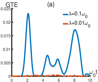
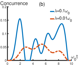
Figure 6: (a) GTE of the three-qubit system is obtained using the numerical HEOM method without RWA both for strong ($\lambda=0.1\omega_{0}$) and ultrastrong coupling ($\lambda=0.01\omega_{0}$) regimes. The initial state is defined as $|\psi(0)\rangle=\ket{ggg}\otimes|0\rangle_{R}$ and the parameters are set as follows: $\gamma=0.01\omega_{0}$, $\omega_{0}=1$, and $\alpha_{1}=\alpha_{2}=\alpha_{3}=1$ . (b) the same as (a), but here the concurrence is obtained for subsystem $\rho_{ab}$, due to the symmetry, we have $\rho_{ab}(t)=\rho_{ac}(t)=\rho_{bc}(t)$. Under the RWA, the initial state does not evolve; both GTE and concurrence stay at zero. Additionally, there is no sudden birth of GTN and BN in three- and two-qubit systems in any case.

In previous studies, researchers have focused on generating quantum entanglement or steering from the initial state $|\psi(0)\rangle=\ket{gg}\otimes|0\rangle_{R}$ for a two-qubit system. Although this type of state does not evolve under the RWA, results indicate that quantum entanglement and steering can be generated through the virtual excitations caused by the counter-rotating wave terms [34, 35, 62]. Therefore, we investigate the effects of counter-rotating wave terms on the GTN and the concurrence of the initial state here. In Fig. 6, for strong coupling cases, one can find that the counter-rotating wave terms can induce GTE and concurrence of the subsystem, but the generated GTE is very weak. For ultrastrong coupling regime, while the concurrence of the subsystem can indeed be generated, GTE is nearly zero during the time evolution. The results suggest that the counter-rotating-wave terms cannot induce entanglement in a three-body system as strongly as it does for a two-body system, reflecting the essential difference between the three-body and the two-body entanglement.

IV Conclusion

In summary, we investigate the effect of counter-rotating-wave terms on the entanglement and BN for $\ket{W}$ and $\ket{ggg}$ qubit state in quantum open systems by comparing the result between the non-RWA and RWA. In non-RWA cases, we use the HEOM approach to study the dynamics of the reduced qubit system. This numerical technique is applicable when the system and the bath are coupled strongly without the treatment of Born-Markovian, perturbative, and rotating-wave approximations. We also obtain the exact time evolution equation of the reduced three-qubit system when RWA is applied. In a comparison of the dynamic evolution of the two methods, the following findings emerged: $(i)$. For the strong coupling regime, the counter-rotating wave terms can suppress the sudden birth amplitude of entanglement and BN in both two- and three-qubit systems. They also enhance the decoherence process of qubit systems, while the RWA fails to predict this phenomenon correctly. $(ii)$. For the strong coupling regime, the sudden birth of BN is observed during the evolution of the two-qubit state when the coupling strength between each qubit and the bath is unequal. This phenomenon occurs because information dissipated can return to the qubit more efficiently with higher coupling strength. $(iii)$. For the ultrastrong coupling regime, the counter-rotating wave terms enhance the sudden birth amplitude of GTN but weaken that of GTE, which indicates that the counter-rotating wave terms play distinctly different roles in various quantum correlations. $(iv)$. The transfer of BN between two- and three-qubit systems is consistently observed, satisfying the principles of complementarity and monogamy in multi-party nonlocality in the ultrastrong coupling regime. $(v)$. For the zero-excitation cases, the counter-rotating wave terms can generate concurrence in the two-qubit system. However, the induced GTE is nearly zero in both strong and ultrastrong coupling regimes, suggesting that virtual excitations are limited in generating genuine three-party correlations. Finally, the recent advancements in experiments related to preparing the various quantum states and engineering strong coupling in superconducting circuits and atom-cavity coupled systems have led us to believe that our findings will be valuable for various experimental applications in quantum computing and quantum information processing.

Appendix A HEOM

In this appendix, we briefly outline the steps for using HEOM to analyze the reduced dynamics of an arbitrary three-qubit system interacting with a bosonic bath. For a generalized quantum dissipative system resulting from interactions with heat baths composed of harmonic oscillators, the total Hamiltonian can be expressed as follows [44]:

$$\hat{H}_{\text{tot}} =\hat{H}_{S}+\hat{H}_{I+B}$$

$$\hat{H}_{I+B} =\sum_{a}\sum_{j=1}^{N_{a}}\left[\frac{\left(\hat{p}_{j}^{a}\right)^{2}}{2m_{j}^{a}}+\frac{1}{2}m_{j}^{a}\left(\omega_{j}^{a}\right)^{2}\left(\hat{x}_{j}^{a}\right)^{2}-\alpha_{j}^{a}\hat{V}^{a}\hat{x}_{j}^{a}\right]$$ (13)

where $\hat{H}_{S}$ refers to the Hamiltonian of the system. The term $\hat{H}_{I+B}$ includes both the bath and the system-bath interaction Hamiltonian. The degrees of freedom of the bath, denoted as $\alpha$, are represented as $N_{\alpha}$ harmonic oscillators. Specifically, the $\alpha$th heat bath is characterized by the following parameters: momentum $\hat{p}_{j}^{a}$, position $\hat{x}_{j}^{a}$, frequencies $\omega_{j}^{a}$, coupling coefficients $\alpha_{j}^{a}$, and masses $m_{j}^{a}$. Additionally, both $\hat{H}_{S}$ and $\hat{V}^{a}$ can be expressed in the following form within the discretized energy spaces

$$\hat{V}^{a}=\sum_{j,k}\hat{V}_{jk}^{a}|j\rangle\langle k|$$ (14)

$$\hat{H}_{A}=\sum_{j}\hbar\omega_{j}|j\rangle\langle j|+\sum_{j\neq k}\hbar\Delta_{jk}(t)|j\rangle\langle k|$$ (15)

here $\ket{j}$ is defined as the $j^{th}$ eigenenergy states of ${H}_{S}$. The spin-boson model we studied is a simplified version with the Eq. (A), with $\alpha=1$ and $j=0,1$.

Then, the exact solution of the reduced quantum subsystem, including all orders of the system-bath interactions, can be derived by making use of the superoperator technique, which can be derived as [63]

$$\hat{\rho}_{S}^{I}(t)= \hat{\mathcal{T}}\exp\big{\{}-\int_{0}^{t}dt_{2}\int_{0}^{t_{2}}dt_{1}\hat{V}\left(t_{2}\right)^{\times}\big{[}C^{R}\left(t_{2}-t_{1}\right)\hat{V}\left(t_{1}\right)^{\times}$$

$$+ iC^{I}\left(t_{2}-t_{1}\right)\hat{V}\left(t_{1}\right)^{\circ}\big{]}\big{\}}\hat{\rho_{S}}(0)$$ (16)

where $\hat{\rho}_{S}^{I}(t)$ is the reduced density matrix of system in the interaction picture. Here, we consider the initial density matrix of the total system $\hat{\rho}_{tot}(0)=\hat{\rho}_{S}(0)\otimes\rho_{B}$, with $\hat{\rho}_{B}=\exp\left(-\beta H_{B}\right)/Z_{B}$ is the initial state of the bath. The superoperators $\hat{V}^{\times}$ and $\hat{V}^{\circ}$ correspond to commute and anti-commute operations, respectively. At zero temperature, with the cavity initially in a vacuum state, the bath correlation function from Eq. (8) can be decomposed into real and imaginary parts:

$$C^{R}(t_{2}-t_{1})=\sum_{k=1}^{2}\frac{\lambda}{2}e^{-\nu_{k}(t_{2}-t_{1})}$$

$$C^{I}(t_{2}-t_{1})=\sum_{k=1}^{2}(-1)^{k}\frac{\lambda}{2i}e^{-\nu_{k}(t_{2}-t_{1})}$$ (17)

where $\nu_{k}=\gamma+(-1)^{k}i\omega_{0}$ and $\omega_{0}$ is the characteristic frequency of the system.

After inserting the correlation function Eq. (A) into Eq. (A) and repeatedly time deriving Eq. (A), the HEOM for the spin-boson model is expressed as (More detail in Ref. [34])

$$\frac{d}{dt}\hat{\rho}_{l}(t)= \left(-i\hat{H}_{s}^{\times}-\vec{l}\cdot\vec{v}\right)\hat{\rho}_{\bar{l}}(t)+\hat{\Phi}\sum_{p=1}^{2}\hat{\rho}_{\vec{l}+\vec{e}_{p}}(t)$$ (18)

$$+\sum_{p=1}^{2}l_{p}\hat{\Psi}_{p}\hat{\rho}_{\vec{l}-\vec{e}_{p}}(t)$$

with

$$\hat{\Phi}=-i{V}^{\times},~{}~{}\hat{\Psi}_{p}=-\frac{i}{2}\lambda\left[\hat{V}^{\times}+(-1)^{p}\hat{V}^{\circ}\right],$$ (19)

here ${l}=(l_{1},l_{2})$ is a two-dimensional index, $\vec{v}=(\gamma-i\omega_{0},\gamma+i\omega_{0})$ is a two-dimensional vector, $\vec{e}_{1}=(1,0)$ and $\vec{e}_{2}=(0,1)$. Besides, $\hat{\rho}_{\vec{l}=({0,0})}(0)=\hat{\rho}_{s}(0)$ is the reduced density matrix of system and $\hat{\rho}_{\vec{l}\neq({0,0})}$ is the auxiliary matrices with all elements are zero at initial moment.

The Eq. (18) can be solved by standard numerical methods, such as the fourth-order Runge-kuta method, after the hierarchical equations are truncated for a sufficiently large integer L(e.g. $\hat{\rho}_{\vec{l}=(l_{1},l_{2})}(t)$ with $l_{1}+l_{2}>L$ will be dropped). In addition, to demonstrate the validity of our HEOM program, we rigorously compared our results with those of Ma Ji et al.’s work [34], which showed a high degree of agreement in Fig. 7

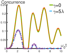
Figure 7: The time evolution of the concurrence is calculated by our numerical HEOM program and the results from Ma Ji et al. [34] for various parameters: $\lambda=0$ (our numerical result: green solid line; Ma Ji et al.’s result: red points), $\lambda=5\lambda$(our numerical result: blue solid line; Ma Ji et al.’s result: purple pentagrams); All other parameters are set to $\lambda=0.1\omega_{0}$ and $\omega_{0}=1$.

Appendix B The exact dynamic equation of three qubits in a common bath under the RWA

In this section, we aim to derive the steps needed to obtain the exact time evolution equation for the reduced three-qubit system under the RWA. To simplify the expression of the equation, we define the collective coupling constant $\alpha_{T}=\left(\alpha_{1}^{2}+\alpha_{2}^{2}+\alpha_{3}^{2}\right)^{1/2}$ and the relative strengths $r_{j}=\alpha_{j}/\alpha_{T}$. By using the scheme proposed in Ref. [38], we can obtain three integrodifferential equations for amplitudes $c_{j}(t)$ (j=1,2,3) as follow:

$$\dot{c}_{1}(t)= -\int_{0}^{t}dt_{1}\left[\alpha_{1}^{2}c_{1}\left(t_{1}\right)+\alpha_{1}\alpha_{2}c_{2}\left(t_{1}\right)+\alpha_{1}\alpha_{3}c_{3}\left(t_{1}\right)\right]$$ (20)

$$\times f\left(t-t_{1}\right),$$

$$\dot{c}_{2}(t)= -\int_{0}^{t}dt_{1}\left[\alpha_{1}\alpha_{2}c_{1}\left(t_{1}\right)+\alpha_{2}^{2}c_{2}\left(t_{1}\right)+\alpha_{2}\alpha_{3}c_{3}\left(t_{1}\right)\right]$$

$$\times f\left(t-t_{1}\right),$$

$$\dot{c}_{3}(t)= -\int_{0}^{t}dt_{1}\left[\alpha_{1}\alpha_{3}c_{1}\left(t_{1}\right)+\alpha_{2}\alpha_{3}c_{2}\left(t_{1}\right)+\alpha_{3}^{2}c_{3}\left(t_{1}\right)\right]$$

$$\times f\left(t-t_{1}\right),$$

where the correlation function $f\left(t-t_{1}\right)$ is defined as the Fourier transform of the spectral density $J(\omega)$ and we can derive the quantities $c_{j}(t)$ by performing the Laplace transform of Eqs. (20) yield

$$s\widetilde{c}_{1}(s)-c_{1}(0)= -\left[\alpha_{1}^{2}\widetilde{c}_{1}(s)+\alpha_{1}\alpha_{2}\widetilde{c}_{2}\left(s\right)+\alpha_{1}\alpha_{3}\widetilde{c}_{3}\left(s\right)\right]$$ (21)

$$\times\widetilde{f}\left(s\right),$$

$$s\widetilde{c}_{2}(s)-c_{2}(0)= -\left[\alpha_{1}\alpha_{2}\widetilde{c}_{1}\left(s\right)+\alpha_{2}^{2}\widetilde{c}_{2}(s)+\alpha_{2}\alpha_{3}\widetilde{c}_{3}\left(s\right)\right]$$

$$\times\widetilde{f}\left(s\right),$$

$$s\widetilde{c}_{3}(s)-c_{3}(0)= -\left[\alpha_{1}\alpha_{3}\widetilde{c}_{1}\left(s\right)+\alpha_{2}\alpha_{3}\widetilde{c}_{2}(s)+\alpha_{3}^{2}\widetilde{c}_{3}\left(s\right)\right]$$

$$\times\widetilde{f}\left(s\right).$$

In order to simplify the solution of the equation, we define $\left|\psi_{+}\right\rangle=r_{1}|1\rangle_{1}|0\rangle_{2}|0\rangle_{3}+r_{2}|0\rangle_{1}|1\rangle_{2}|0\rangle_{3}+r_{3}|0\rangle_{1}|0\rangle_{2}|1\rangle_{3}$ with a structure analogous to the solution of the case presented in Ref. and $\mathcal{E}(t)=\left\langle\psi_{+}\mid\psi_{+}(t)\right\rangle$ is given by

$$\mathcal{E}(t) =e^{-\lambda t/2}\left[\cosh(\Omega t/2)+\frac{\lambda}{\Omega}\sinh(\Omega t/2)\right],$$ (22)

Here $\Omega=\sqrt{\lambda^{2}-4\mathcal{R}^{2}}$. With the help of the expression of $\mathcal{E}(t)$, we can get the exact solution of the probability amplitude $c_{j}$ as

$$c_{1}(t) =\left[r_{2}^{2}+r_{3}^{2}+r_{1}^{2}\mathcal{E}(t)\right]c_{1}(0)-r_{1}r_{2}[1-\mathcal{E}(t)]c_{2}(0)$$ (23)

$$-r_{1}r_{3}[1-\mathcal{E}(t)]c_{3}(0),$$

$$c_{2}(t) =\left[r_{1}^{2}+r^{2}_{3}+r_{2}^{2}\mathcal{E}(t)\right]c_{2}(0)-r_{1}r_{2}[1-\mathcal{E}(t)]c_{1}(0)$$

$$-r_{2}r_{3}[1-\mathcal{E}(t)]c_{3}(0),$$

$$c_{3}(t) =\left[r_{1}^{2}+r_{2}^{2}+r_{3}^{2}\mathcal{E}(t)\right]c_{3}(0)-r_{1}r_{3}[1-\mathcal{E}(t)]c_{1}(0)$$

$$-r_{2}r_{3}[1-\mathcal{E}(t)]c_{2}(0).$$

Thus, the evolution of the entanglement dynamics in the system is influenced by the coupling strength $r_{j}$ and the initial state $c_{j}(0)$.

References

- Einstein et al. [1935] A. Einstein, B. Podolsky, and N. Rosen, Can quantum-mechanical description of physical reality be considered complete?, Phys. Rev. 47, 777 (1935).
- Bell [1964] J. S. Bell, On the einstein podolsky rosen paradox, Physics Physique Fizika 1, 195 (1964).
- Brunner et al. [2014] N. Brunner, D. Cavalcanti, S. Pironio, V. Scarani, and S. Wehner, Bell nonlocality, Rev. Mod. Phys. 86, 419 (2014).
- Shalm et al. [2021] L. K. Shalm, Y. Zhang, J. C. Bienfang, C. Schlager, M. J. Stevens, M. D. Mazurek, C. Abellán, W. Amaya, M. W. Mitchell, M. A. Alhejji, et al., Device-independent randomness expansion with entangled photons, Nature Physics 17, 452 (2021).
- Li et al. [2021] M.-H. Li, X. Zhang, W.-Z. Liu, S.-R. Zhao, B. Bai, Y. Liu, Q. Zhao, Y. Peng, J. Zhang, Y. Zhang, W. J. Munro, X. Ma, Q. Zhang, J. Fan, and J.-W. Pan, Experimental realization of device-independent quantum randomness expansion, Phys. Rev. Lett. 126, 050503 (2021).
- Zhang et al. [2024] Y. Zhang, Y. Bian, Z. Li, S. Yu, and H. Guo, Continuous-variable quantum key distribution system: Past, present, and future, Applied Physics Reviews 11, 011318 (2024).
- Ekert [1991] A. K. Ekert, Quantum cryptography based on bell’s theorem, Phys. Rev. Lett. 67, 661 (1991).
- Bennett et al. [1993] C. H. Bennett, G. Brassard, C. Crépeau, R. Jozsa, A. Peres, and W. K. Wootters, Teleporting an unknown quantum state via dual classical and einstein-podolsky-rosen channels, Phys. Rev. Lett. 70, 1895 (1993).
- Su et al. [2020] Z. Su, H. Tan, and X. Li, Entanglement as upper bound for the nonlocality of a general two-qubit system, Phys. Rev. A 101, 042112 (2020).
- Brito et al. [2018] S. G. A. Brito, B. Amaral, and R. Chaves, Quantifying bell nonlocality with the trace distance, Phys. Rev. A 97, 022111 (2018).
- Elben et al. [2020] A. Elben, R. Kueng, H.-Y. R. Huang, R. van Bijnen, C. Kokail, M. Dalmonte, P. Calabrese, B. Kraus, J. Preskill, P. Zoller, and B. Vermersch, Mixed-state entanglement from local randomized measurements, Phys. Rev. Lett. 125, 200501 (2020).
- Gour and Scandolo [2020] G. Gour and C. M. Scandolo, Dynamical entanglement, Phys. Rev. Lett. 125, 180505 (2020).
- Dür et al. [2000] W. Dür, G. Vidal, and J. I. Cirac, Three qubits can be entangled in two inequivalent ways, Phys. Rev. A 62, 062314 (2000).
- Xie and Eberly [2021] S. Xie and J. H. Eberly, Triangle measure of tripartite entanglement, Phys. Rev. Lett. 127, 040403 (2021).
- Li and Shang [2022] Y. Li and J. Shang, Geometric mean of bipartite concurrences as a genuine multipartite entanglement measure, Phys. Rev. Res. 4, 023059 (2022).
- Dong et al. [2024] D.-D. Dong, L.-J. Li, X.-K. Song, L. Ye, and D. Wang, Quantifying genuine tripartite entanglement by reshaping the state, Phys. Rev. A 110, 032420 (2024).
- Ma et al. [2011] Z.-H. Ma, Z.-H. Chen, J.-L. Chen, C. Spengler, A. Gabriel, and M. Huber, Measure of genuine multipartite entanglement with computable lower bounds, Phys. Rev. A 83, 062325 (2011).
- Svetlichny [1987] G. Svetlichny, Distinguishing three-body from two-body nonseparability by a bell-type inequality, Phys. Rev. D 35, 3066 (1987).
- Ajoy and Rungta [2010] A. Ajoy and P. Rungta, Svetlichny’s inequality and genuine tripartite nonlocality in three-qubit pure states, Phys. Rev. A 81, 052334 (2010).
- Ghose et al. [2009] S. Ghose, N. Sinclair, S. Debnath, P. Rungta, and R. Stock, Tripartite entanglement versus tripartite nonlocality in three-qubit greenberger-horne-zeilinger-class states, Phys. Rev. Lett. 102, 250404 (2009).
- Huang et al. [2022] L. Huang, X.-M. Gu, Y.-F. Jiang, D. Wu, B. Bai, M.-C. Chen, Q.-C. Sun, J. Zhang, S. Yu, Q. Zhang, C.-Y. Lu, and J.-W. Pan, Experimental demonstration of genuine tripartite nonlocality under strict locality conditions, Phys. Rev. Lett. 129, 060401 (2022).
- Kang et al. [2016] Y.-H. Kang, Y.-H. Chen, Q.-C. Wu, B.-H. Huang, J. Song, and Y. Xia, Fast generation of w states of superconducting qubits with multiple schrödinger dynamics, Scientific reports 6, 36737 (2016).
- Wei and Chen [2015] X. Wei and M.-F. Chen, Preparation of multi-qubit w states in multiple resonators coupled by a superconducting qubit via adiabatic passage, Quantum Information Processing 14, 2419 (2015).
- Neeley et al. [2010] M. Neeley, R. C. Bialczak, M. Lenander, E. Lucero, M. Mariantoni, A. O’connell, D. Sank, H. Wang, M. Weides, J. Wenner, et al., Generation of three-qubit entangled states using superconducting phase qubits, Nature 467, 570 (2010).
- Sami et al. [2017] S. Sami, I. Chakrabarty, and A. Chaturvedi, Complementarity of genuine multipartite bell nonlocality, Phys. Rev. A 96, 022121 (2017).
- Arnon-Friedman et al. [2018] R. Arnon-Friedman, F. Dupuis, O. Fawzi, R. Renner, and T. Vidick, Practical device-independent quantum cryptography via entropy accumulation, Nature communications 9, 459 (2018).
- Jozsa and Linden [2003] R. Jozsa and N. Linden, On the role of entanglement in quantum-computational speed-up, Proceedings of the Royal Society of London. Series A: Mathematical, Physical and Engineering Sciences 459, 2011 (2003).
- Rodriguez-Blanco et al. [2021] A. Rodriguez-Blanco, A. Bermudez, M. Müller, and F. Shahandeh, Efficient and robust certification of genuine multipartite entanglement in noisy quantum error correction circuits, PRX Quantum 2, 020304 (2021).
- Breuer and Petruccione [2002] H.-P. Breuer and F. Petruccione, The theory of open quantum systems (Oxford University Press, USA, 2002).
- de Vega and Alonso [2017] I. de Vega and D. Alonso, Dynamics of non-markovian open quantum systems, Rev. Mod. Phys. 89, 015001 (2017).
- Nielsen and Chuang [2010] M. A. Nielsen and I. L. Chuang, Quantum computation and quantum information (Cambridge university press, 2010).
- Weiss [2012] U. Weiss, Quantum dissipative systems (World Scientific, 2012).
- Wu and Liu [2017] W. Wu and M. Liu, Effects of counter-rotating-wave terms on the non-markovianity in quantum open systems, Phys. Rev. A 96, 032125 (2017).
- Ma et al. [2012] J. Ma, Z. Sun, X. Wang, and F. Nori, Entanglement dynamics of two qubits in a common bath, Phys. Rev. A 85, 062323 (2012).
- Sun et al. [2018] Z. Sun, X.-Q. Xu, and B. Liu, Creation of quantum steering by interaction with a common bath, Phys. Rev. A 97, 052309 (2018).
- Maniscalco et al. [2008] S. Maniscalco, F. Francica, R. L. Zaffino, N. Lo Gullo, and F. Plastina, Protecting entanglement via the quantum zeno effect, Phys. Rev. Lett. 100, 090503 (2008).
- Nourmandipour et al. [2016] A. Nourmandipour, M. K. Tavassoly, and M. A. Bolorizadeh, Quantum zeno and anti-zeno effects on the entanglement dynamics of qubits dissipating into a common and non-markovian environment, J. Opt. Soc. Am. B 33, 1723 (2016).
- Francica et al. [2009] F. Francica, S. Maniscalco, J. Piilo, F. Plastina, and K.-A. Suominen, Off-resonant entanglement generation in a lossy cavity, Phys. Rev. A 79, 032310 (2009).
- Cao et al. [2010] X. Cao, J. Q. You, H. Zheng, A. G. Kofman, and F. Nori, Dynamics and quantum zeno effect for a qubit in either a low- or high-frequency bath beyond the rotating-wave approximation, Phys. Rev. A 82, 022119 (2010).
- Zheng et al. [2008] H. Zheng, S. Y. Zhu, and M. S. Zubairy, Quantum zeno and anti-zeno effects: Without the rotating-wave approximation, Phys. Rev. Lett. 101, 200404 (2008).
- Ai et al. [2010] Q. Ai, Y. Li, H. Zheng, and C. P. Sun, Quantum anti-zeno effect without rotating wave approximation, Phys. Rev. A 81, 042116 (2010).
- Tanimura and Kubo [1989] Y. Tanimura and R. Kubo, Time evolution of a quantum system in contact with a nearly gaussian-markoffian noise bath, Journal of the Physical Society of Japan 58, 101 (1989).
- Xu and Yan [2007] R.-X. Xu and Y. Yan, Dynamics of quantum dissipation systems interacting with bosonic canonical bath: Hierarchical equations of motion approach, Phys. Rev. E 75, 031107 (2007).
- Tanimura [2020] Y. Tanimura, Numerically “exact” approach to open quantum dynamics: The hierarchical equations of motion (HEOM), The Journal of Chemical Physics 153, 020901 (2020).
- Dijkstra and Tanimura [2010] A. G. Dijkstra and Y. Tanimura, Non-markovian entanglement dynamics in the presence of system-bath coherence, Phys. Rev. Lett. 104, 250401 (2010).
- Wu and Lin [2017] W. Wu and H.-Q. Lin, Quantum zeno and anti-zeno effects in quantum dissipative systems, Phys. Rev. A 95, 042132 (2017).
- Wu and Lin [2016] W. Wu and H.-Q. Lin, Effect of bath temperature on the decoherence of quantum dissipative systems, Phys. Rev. A 94, 062116 (2016).
- Vidal and Werner [2002] G. Vidal and R. F. Werner, Computable measure of entanglement, Phys. Rev. A 65, 032314 (2002).
- Ollivier and Zurek [2001] H. Ollivier and W. H. Zurek, Quantum discord: A measure of the quantumness of correlations, Phys. Rev. Lett. 88, 017901 (2001).
- Wootters [1998] W. K. Wootters, Entanglement of formation of an arbitrary state of two qubits, Phys. Rev. Lett. 80, 2245 (1998).
- Wu and Zeng [2022] S.-M. Wu and H.-S. Zeng, Genuine tripartite nonlocality and entanglement in curved spacetime, The European Physical Journal C 82, 4 (2022).
- Clauser et al. [1969] J. F. Clauser, M. A. Horne, A. Shimony, and R. A. Holt, Proposed experiment to test local hidden-variable theories, Phys. Rev. Lett. 23, 880 (1969).
- Guo et al. [2022] Y. Guo, Y. Jia, X. Li, and L. Huang, Genuine multipartite entanglement measure, Journal of Physics A: Mathematical and Theoretical 55, 145303 (2022).
- Coffman et al. [2000] V. Coffman, J. Kundu, and W. K. Wootters, Distributed entanglement, Phys. Rev. A 61, 052306 (2000).
- Ou and Fan [2007] Y.-C. Ou and H. Fan, Monogamy inequality in terms of negativity for three-qubit states, Phys. Rev. A 75, 062308 (2007).
- Torres-Arenas et al. [2019] A. J. Torres-Arenas, Q. Dong, G.-H. Sun, W.-C. Qiang, and S.-H. Dong, Entanglement measures of w-state in noninertial frames, Physics Letters B 789, 93 (2019).
- Xiong et al. [2024] Z.-Y. Xiong, Y.-J. Xiao, Y.-Q. Zhang, and Q.-L. He, Quantum zeno effect on genuine tripartite nonlocality and entanglement in quantum dissipative system, arXiv preprint arXiv:2405.19664 10.48550/arXiv.2405.19664 (2024).
- Kumari et al. [2023] S. Kumari, J. Naikoo, S. Ghosh, and A. K. Pan, Interplay of nonlocality and incompatibility breaking qubit channels, Phys. Rev. A 107, 022201 (2023).
- Wang et al. [2020] K. Wang, Y. Liang, and Z.-J. Zheng, Genuine tripartite nonlocality of ghz state in noninertial frames, Quantum Information Processing 19, 1 (2020).
- Wang and Zheng [2020] K. Wang and Z.-J. Zheng, Violation of svetlichny inequality in triple jaynes-cummings models, Scientific Reports 10, 6621 (2020).
- Salem et al. [2024] V. Salem, A. A. Silva, and F. M. Andrade, Multipartite entanglement sudden death and birth in randomized hypergraph states, Phys. Rev. A 109, 012416 (2024).
- Altintas and Eryigit [2012] F. Altintas and R. Eryigit, Creation of quantum correlations between two atoms in a dissipative environment from an initial vacuum state, Physics Letters A 376, 1791 (2012).
- Tanimura [2006] Y. Tanimura, Stochastic liouville, langevin, fokker-planck, and master equation approaches to quantum dissipative systems, Journal of the Physical Society of Japan 75, 082001 (2006).