DKMGP: A Gaussian Process Approach to Multi-Task and Multi-Step Vehicle Dynamics Modeling in Autonomous Racing

Abstract

Autonomous racing is gaining attention for its potential to advance autonomous vehicle technologies. Accurate race car dynamics modeling is essential for capturing and predicting future states like position, orientation, and velocity. However, accurately modeling complex subsystems such as tires and suspension poses significant challenges. In this paper, we introduce the Deep Kernel-based Multi-task Gaussian Process (DKMGP), which leverages the structure of a variational multi-task and multi-step Gaussian process model enhanced with deep kernel learning for vehicle dynamics modeling. Unlike existing single-step methods, DKMGP performs multi-step corrections with an adaptive correction horizon (ACH) algorithm that dynamically adjusts to varying driving conditions. To validate and evaluate the proposed DKMGP method, we compare the model performance with DKL-SKIP and a well-tuned single-track model, using high-speed dynamics data (exceeding $230\text{\,}\mathrm{km}\text{\,}{\mathrm{h}}^{-1}$) collected from a full-scale Indy race car during the Indy Autonomous Challenge held at the Las Vegas Motor Speedway at CES 2024. The results demonstrate that DKMGP achieves upto 99% prediction accuracy compared to one-step DKL-SKIP, while improving real-time computational efficiency by 1752x. Our results show that DKMGP is a scalable and efficient solution for vehicle dynamics modeling making it suitable for high-speed autonomous racing control.

1 Introduction

As the technology of autonomous vehicles has developed during the past decade, there has been an increased growth of the research in autonomous racing ([Betz et al.(2022)Betz, Zheng, Liniger, Rosolia, Karle, Behl, Krovi, and Mangharam], [Weiss and Behl(2020)]). Competitions in autonomous racing have been held not only in simulators ([Hartmann et al.(2021)Hartmann, Shiller, and Azaria, Babu and Behl(2020)]), but also on hardware with racecars’ ranging from 1:43 scale RC cars, to 1/10 scale F1tenth Racing ([O’Kelly et al.(2019)O’Kelly, Sukhil, Abbas, Harkins, Kao, Pant, Mangharam, Agarwal, Behl, Burgio, et al.]) to full-size Indy racecars ([Carrau et al.(2016)Carrau, Liniger, Zhang, and Lygeros, Wischnewski et al.(2022)Wischnewski, Geisslinger, Betz, Betz, Fent, Heilmeier, Hermansdorfer, Herrmann, Huch, Karle, et al.]). To enable optimal performance, it is essential to learn an accurate vehicle dynamics model for model-based control algorithms. However, the nonlinear nature of vehicle subsystems makes constructing a high-fidelity dynamics model challenging, as first-principles approaches rely on complex mathematical equations to describe these dynamics ([Althoff et al.(2017)Althoff, Koschi, and Manzinger]). Researchers often employ simplified vehicle models to overcome this complexity, such as single-track models. However, these models suffer from over-simplifications and do not fully capture vehicles’ nonlinear behaviors. In addition, first-principles modeling approaches are often costly and time-consuming to develop and fine-tune. For instance, the [Pacejka(2005)] tire model is commonly applied to capture tire-road interactions. Building this model requires parameters obtained from experimental data, such as grip, wear, and temperature changes, necessitating expert knowledge and specialized tire testing rigs to measure forces, torques, and displacements under various conditions.

Related Works: Consequently, researchers are increasingly turning to learning-based modeling approaches based on machine learning to bridge the discrepancy between simplified vehicle models and real dynamics ([Hermansdorfer et al.(2020)Hermansdorfer, Trauth, Betz, and Lienkamp, Da Lio et al.(2020)Da Lio, Bortoluzzi, and Rosati Papini]). [Pan et al.(2021)Pan, Nie, Li, and Gu] proposed Deep Pacejka, a data-driven modeling approach based on deep neural networks (DNNs) for computing and predicting vehicle dynamics. [Chrosniak et al.(2024)Chrosniak, Ning, and Behl] has extended the Deep Pacejka by implementing the physics-informed neural network, which combines the physics coefficient estimation and dynamical equations to predict the vehicle dynamics of a full-sized racecar. Alternatively, hybrid models that combine physics-based insights with data-driven approaches offer a promising middle ground, leveraging the strengths of both methods. [Van Niekerk et al.(2017)Van Niekerk, Damianou, and Rosman] first proposed Gaussian process (GP) models for learning vehicle dynamics, leveraging their interpretability and reliable uncertainty estimates. The use of GP models to predict racecar dynamics by modeling the residuals between simplified models and real-world dynamics has been further investigated by researchers ([Jain et al.(2021)Jain, O’Kelly, Chaudhari, and Morari, Kabzan et al.(2019)Kabzan, Hewing, Liniger, and Zeilinger]). The limitations of previous work of GP-based dynamics learning methods include unrealistic experiment setups, such as small-scaled racecars and the use of made-up racetracks ([Ning and Behl(2024)]). While learning-based controllers using GPs are promising for capturing nonlinear dynamics, their high computational costs and latency, limit their integration into model-based controllers for high-speed applications like autonomous racing. Thus, there is a critical need for efficient learning-based models that can support real-time, closed-loop control strategies.

Contributions: Building upon prior work, [Ning and Behl(2023b)] proposed DKL-SKIP, which effectively predicts model errors in the dynamics of a full-size autonomous racecar. However, this method has two main limitations: it models each state separately, requiring three DNN models to predict all state residuals, and it operates only in a single-step prediction manner. In this paper, we extend the concept of DKL-SKIP and address its limitations by proposing the Deep Kernel-based Multi-task Gaussian Process (DKMGP) model. The contributions of this paper are as follows:

1. We introduce the DKMGP, a multi-task variational Gaussian Process model that can predict all state residuals with a single correction model.

2. DKMGP can be trained for multi-step predictions, needed for closed-loop model-based control. Our second contribution is developing an adaptive correction horizon (ACH) algorithm to reduce inference times for multi-step predictions.

3. We validate DKMGP using high-speed racing data from a full-scale autonomous racecar from the Indy Autonomous Challenge, reaching speeds over $230\text{\,}\mathrm{km}\text{\,}{\mathrm{h}}^{-1}$.

While the DKMGP model presented in this work focuses on enhancing vehicle dynamics prediction and real-time performance; both of these are critical precursors for model-based closed-loop control in autonomous racing. To the best of our knowledge, this is the first work to utilize a learning-enabled multi-task Gaussian Process for vehicle dynamics modeling for autonomous racing.

2 Background and Problem Formulation

We first present a brief overview of the single-track and the E-kin models used in this paper.

Table 1: E-kin model and single-track model state equations; highlighted states differ between the models, including the Pacejka tire model equations

State Variable	Notation	State Equation (E-Kin)	State Equation (Single-track)
Horizontal Position ($\mathrm{m}$)	$x$	$\dot{x}=v_{x}\cos\psi-v_{y}\sin\psi$	$\dot{x}=v_{x}\cos\psi-v_{y}\sin\psi$
Vertical Position ($\mathrm{m}$)	$y$	$\dot{y}=v_{x}\sin\psi_{t}+v_{y}\cos\psi$	$\dot{y}=v_{x}\sin\psi+v_{y}\cos\psi$
Longitudinal Velocity ($\mathrm{m}\text{\,}{\mathrm{s}}^{-1}$)	$v_{x}$	$\dot{v}_{x}$ $=\frac{T_{w}}{l_{r}+l_{f}}a_{x}$	$\dot{v}_{x}$ $=a_{x}$
Lateral Velocity ($\mathrm{m}\text{\,}{\mathrm{s}}^{-1}$)	$v_{y}$	$\dot{v}_{y}$ $=\frac{1}{T_{w}(l_{r}+l_{f})}(a_{x}\sin\psi+v_{x}\omega)$	$\dot{v}_{y}$ $=\frac{1}{m}(F_{ry}+F_{fy}\cos\delta-F_{by})-v_{x}\omega$
Inertial Heading ($\mathrm{rad}$)	$\psi$	$\dot{\psi}=\omega$	$\dot{\psi}=\omega$
Steering Angle ($\mathrm{rad}$)	$\delta$	$\dot{\delta}=\Delta\delta$	$\dot{\delta}=\Delta\delta$
Yaw Rate ($\mathrm{rad}\text{\,}{\mathrm{s}}^{-1}$)	$\omega$	$\dot{\omega}$ $=\frac{h_{cog}}{T_{w}(l_{r}+l_{f})}(a_{x}\cos\psi+v_{x}\omega)$	$\dot{\omega}$ $=\frac{1}{I_{z}}(l_{f}F_{fy}\cos\delta-l_{r}F_{ry})$
Tire Forces (Pacejka)
Front Lateral Tire Force ($\mathrm{N}$)	$F_{yf}$	$F_{yf}=Svy_{f}+D_{f}\sin(C_{f}\arctan(B_{f}\alpha_{f}-E_{f}(B_{f}\alpha_{f}-\arctan(B_{f}\alpha_{f}))))$
Rear Lateral Tire Force ($\mathrm{N}$)	$F_{yr}$	$F_{yr}=Svy_{r}+D_{r}\sin(C_{r}\arctan(B_{r}\alpha_{r}-E_{r}(B_{r}\alpha_{r}-\arctan(B_{r}\alpha_{r}))))$
Front Slip Angle ($\mathrm{rad}$)	$\alpha_{f}$	$\alpha_{f}=\alpha_{f0}+Shy_{f},\quad\alpha_{f0}=\delta-\arctan\left(\frac{v_{y}+l_{f}\omega}{v_{x}}\right)$
Rear Slip Angle ($\mathrm{rad}$)	$\alpha_{r}$	$\alpha_{r}=\alpha_{r0}+Shy_{r},\quad\alpha_{r0}=-\arctan\left(\frac{v_{y}-l_{r}\omega}{v_{x}}\right)$

2.1 Single-track Model

The single-track model, as shown in Fig.1, simplifies the vehicle dynamics by combining the two wheels of both the front and rear axles into a single wheel per axle. This model is commonly used for motion planning and real-time vehicle control ([Raji et al.(2022)Raji, Liniger, Giove, Toschi, Musiu, Morra, Verucchi, Caporale, and Bertogna, Liniger et al.(2015)Liniger, Domahidi, and Morari].) The differential equations of state descriptions of the single-track model are shown in the Table 1, where the vehicle state is composed of $s=\{x,y,v_{x},v_{y},\psi,$ $\delta,\omega\}$, and the inputs are $u=\{a_{x},\Delta\delta\}$, where $\Delta\delta$ represents the steering velocity, $a_{x}$ is the longitudinal vehicle acceleration, respectively. Note that in this work, we simplify the longitudinal dynamics by directly using the vehicle’s longitudinal acceleration, whereas in real-world applications, a well-calibrated drivetrain model is necessary to precisely compute the force transferred from the engine to the driving wheels. The lateral dynamics of the racecar are characterized by states including lateral velocity ($v_{y}$), yaw rate ($\psi$), steering angle ($\delta$), and yaw rate ($\omega$). The associated differential equations incorporate forces such as the lateral tire forces of the front ($F_{fy}$) and rear ($F_{ry}$) axles, and the force due to bank angle ($F_{b_{y}}$), where $F_{b_{y}}=mg\sin(\theta)$ approximates the influence of the bank angle $\theta$. Tire forces, $F_{fy}$ and $F_{ry}$, are modeled using the Pacejka magic formula for the tire model, detailed in the bottom of Table 1.

2.2 Extended Kinematic Model

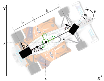
Figure 1: The single-track vehicle model of the racecar, with all three base states $(v_{x}.v_{y},\omega)$ highlighted.

Table 1 demonstrates that all vehicle states can be derived from the base states $\{v_{x},v_{y},\omega\}$. While the single-track model simplifies vehicle dynamics modeling, it still requires extensive expert knowledge and calibration. For instance, deriving $\dot{v}_{y}$ involves lateral dynamics influenced by aerodynamics and tire forces, while $\dot{v}_{x}$ requires understanding of the powertrain system. To reduce model development costs, we propose an extended kinematic single-track (E-kin) model, shown in column 3 of Table 1. Unlike the nonlinear single-track model, which relies on detailed subsystem modeling, the E-kin model approximates the derivatives of the base states using measurable variables such as $a_{x}$, $\psi$, and $\delta$. This approach avoids explicit modeling of complex subsystems like tire dynamics and drivetrain dynamics, greatly simplifying and reducing modeling costs. However, the E-kin model’s simplifications introduce discrepancies between its predictions and real-world vehicle dynamics. Thus, a method is needed to learn and compensate for these mismatches while retaining the model’s simplified calibration benefits.

2.3 Problem Formulation

Given a dataset $D=\{d_{1},d_{2},\dots,d_{N}\}$ consisting of $N$ vehicle state measurement samples $S=\{s_{1},s_{2},\dots,s_{N}\}$ and inputs $U=\{u_{1},u_{2},\dots,u_{N}\}$, the objective is to predict future states $\hat{s}_{t+1},\ldots,\hat{s}_{t+n}$ using a learned model that corrects for the inaccuracies in the baseline E-kin model.

Problem 1: Model Error Correction The dynamics predicted by a simplified model, $\hat{s}_{t+1}$, are generated by propagating the E-kin model with the inputs $u_{t}=\{a_{x,t},\Delta\delta_{t}\}$ and initial states $s_{t}=\{x_{t},y_{t},v_{x,t},v_{y,t},\psi_{t},\delta_{t},\omega_{t}\}$. These predictions, that we will denote with $f_{\text{E-kin}}(s_{t},u_{t})$, deviate from the true system behavior $s_{t+1}$, due to unmodeled complexities. Define the model residual at time $t+1$ as $r_{t+1}=s_{t+1}-f_{Ekin}(s_{t},u_{t})$, where $r_{t+1}=[0,0,\epsilon_{v_{x},t+1},\epsilon_{v_{y},t+1},0,0,\epsilon_{\omega,t+1}]$ captures the errors $\epsilon$ in predicting the base dynamic states $\{v_{x},v_{y},\omega\}$ at time $t+1$. Our goal is to learn a model $f_{\text{corr}}$ that corrects the baseline predictions using these residuals:

$$f_{\text{corr}}(s_{t+1},u_{t+1})=f_{\text{E-kin}}(s_{t},u_{t})+\mathbf{e}_{t+1},$$ (1)

where $\mathbf{e}_{t}=\{\epsilon_{v_{x},t},\epsilon_{v_{y},t},\epsilon_{\omega,t}\}$ represents the estimated model error, $r_{t}$, which is estimated using a Gaussian Process (GP) model: $\mathbf{e}_{t}=\mathcal{GP}(d_{t-1})+\nu_{t},\quad\nu_{t}\sim\mathcal{N}(0,\sigma^{2})$, with the previous state measurement $d_{t-1}$ as the input. Existing GP-based models, such as DKL-SKIP ([Ning and Behl(2023a)]), predict each correction state independently, resulting in high computational costs due to the space and time complexity of GP models. The challenge in this paper is to use a single correction model to improve the suitability of the method for closed-loop control. We leverage correlations between the base state variables $\{v_{x},v_{y},\omega\}$ using a Multi-Task Gaussian Process (MTGP) model, that predicts all model errors simultaneously.

Problem 2: Multi-Step Prediction The objective in multi-step prediction is, at time $t$, to predict future states over a given prediction horizon $m$ i.e.

$$\begin{array}[]{ccc}\hat{s}_{t+1}=f_{Ekin}(s_{t},u_{t});&\dots;&\hat{s}_{t+m}=f_{Ekin}(\hat{s}_{t+m-1},u_{t+m-1})\\ \end{array}$$ (2)

However, auto-regressive propagation of the E-Kin model leads to significant deviations, between the prediction $\hat{s}_{t+m}$ and the true state $s_{t+m}$, at the end of the prediction horizon. Additionally, one can keep correcting the model prediction at each step of the horizon but that is computationally prohibitive. Therefore, we need to learn an MTGP model that can correct the deviations at fixed intervals that we term as the correction horizon, $n$, for the MTGP model, with $n<m$. The MTGP model needs to directly correct the $n^{th}$ prediction, following $(n-1)$ E-Kin model propagations:

$$\hat{s}_{t+n}=f_{\text{E-kin}}(\hat{s}_{t+n-1},u_{t+n-1})+\mathbf{e}_{t+n},$$ (3)

$\mathbf{e}_{t+n}$ is estimated using the DKMGP framework presented next. Choosing good values for the correction horizon $n$, itself is also a problem of interest for our work.

3 DKMGP Methodology

This section details the methodology of the proposed DKMGP model, depicted in Figure 3. The model integrates a deep neural network (DNN) with a multi-task variational Gaussian Process (MTGP). The DNN serves as a feature extractor, adept at capturing non-linear relationships and extracting relevant information from the input data. The MTGP employs a Linear Model of Coregionalization (LMC) within a variational framework to predict multiple targets simultaneously.

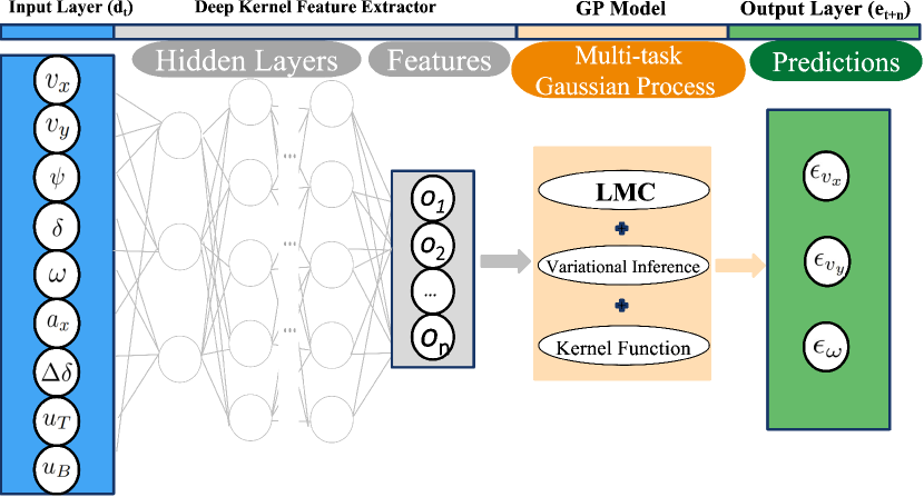
Figure 2: The architecture of the DKMGP model.

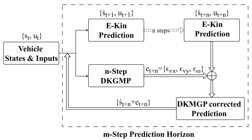
Figure 3: Workflow of the multi-step approach for the DKMGP predictions.

3.1 Deep Kernel Learning

Gaussian process regression, as a non-parametric method, does not learn new representations of the data. Instead, it utilizes a predetermined kernel function to measure the similarity between data points ([Rasmussen(2003)]). Specifically, rather than transforming or adapting the input data into a new feature space, as seen in the neural network models, GP defines a fixed feature space determined by the selected kernel function and its hyperparameters. Therefore, the limited expressiveness and adaptability of GP methods make it challenging for them to capture complex relationships between variables in highly nonlinear and dynamic environments, such as autonomous racing as shown in previous work of [Ning and Behl(2024)]. To address this, we use the deep kernel learning (DKL) method aiming to transform a standard kernel $k(d_{i},d_{j}|\theta)$ to a deep kernel through a neural network, $g(\cdot)$, as denoted in Equation 4.

$$k(d_{i},d_{j};\theta)\rightarrow k(g(d_{i},w),g(d_{j},w)|\theta,w)\mbox{\makebox[0.0pt][l]{\raisebox{2.31895pt}{$\approx$}}$\approx$}k(\tilde{d}_{i},\tilde{d}_{j};\gamma)$$ (4)

Here, $g(d,w)$ denotes a deep neural network with weights $w$, while $\theta$ represents the hyperparameters of GP kernel, such as the length-scale $l$ in an RBF kernel. To learn data representations, the collective hyperparameters for the deep kernel, denoted as $\gamma=\{\theta,w\}$, can be jointly learned and optimized. Furthermore, since DKL serves as a feature extractor, its transformation enables DKL to capture the most relevant features from the input data while simultaneously reducing its dimensionality. Specifically, it maps each input sample $d\in\mathbb{R}^{9}$ to a lower-dimensional feature representation $\tilde{d}\in\mathbb{R}^{4}$, thereby reducing the computational burden of GP models, as expressed in Equation 4.

3.2 Multi-Task Gaussian Process

Different from single-task Gaussian Process, in the context of the MTGP model, we consider a dataset $D$ comprising $N$ distinct inputs, denoted as $\{d_{1},\dots,d_{N}\}$, and associated with these inputs are outcomes corresponding to Multiple tasks. There are three tasks in this paper, denoted as $\{\epsilon_{v_{x}},\epsilon_{v_{y}},\epsilon_{\omega}\}$, which are derived from the model residuals of the base states. These tasks are represented as $\{\epsilon_{v_{x,1}},\dots,\epsilon_{v_{x,N}};\epsilon_{v_{y,1}},\dots,\epsilon_{v_{y,N}};\epsilon_{\omega_{1}},\dots,\epsilon_{\omega_{N}}\}$, forming an $T\times N$ matrix, where $T=3$ and each element corresponds to the response of a task to the $i^{th}$ input $d_{i}$.

Linear model of coregionalization Given that the model residuals of the vehicle base states {$v_{x}$, $v_{y}$, $\omega$} are correlated, where changes in one state affect the others due to the physical interactions between the vehicle’s dynamics, we apply the linear model of coregionalization (LMC) method to capture these correlations across the tasks. The goal of LMC is to leverage the correlation across different tasks to improve prediction accuracy and learning efficiency, thus providing a robust framework for MTGP. Instead of assuming that each task is independent, LMC models the tasks as being correlated through one or more latent functions. For instance, LMC assumes that the $T$ task-specific functions $f_{1},f_{2},\dots,f_{T}$ are generated from a smaller number of latent function $h_{1},\dots,h_{Q}$, which induce correlations between the tasks ([Alvarez et al.(2012)Alvarez, Rosasco, Lawrence, et al.]). Therefore, for the dataset with $T$ tasks and $Q$ latent functions, the MTGP for the $\tau$-th task at input $d_{i}$ is expressed as: $f_{\tau}(d_{i})=\sum_{q=1}^{Q}a_{\tau q}h_{q}(d_{i})+\nu_{\tau}$. where $h_{q}$ are GP latent functions with zero mean and covariance $h_{q}(d_{i})\sim\mathcal{GP}(0,k_{q}(d_{i},d_{j}))$. Task similarities are established through the mixing coefficients $a_{\tau q}$, which determine how the latent functions contribute to each task’s output. $\nu_{\tau}$ represents independent noise for the $\tau$-th task. The covariance between any two tasks $\tau$ and $\tau^{\prime}$ at inputs $d_{i}$ and $d_{j}$ is given by: $Cov(f_{\tau}(d_{i}),f_{\tau^{\prime}}(d_{j}))=\sum_{j=1}^{q}a_{\tau q}a_{\tau^{\prime}q}k_{q}(d_{i},d_{j})$. Therefore, under the LMC framework and the assumption of $Q$ independent latent GP functions, the vector-valued function $F(d_{i})=[f_{1}(d_{i});...;f_{\tau}(d_{i})]$ follows a GP prior defined as:$F(d_{i})\sim\mathcal{GP}(0,\sum_{q=1}^{Q}A_{q}k_{q}(d_{i},d_{j}))$. Where $A_{q}\in R^{T\times T}$ is known as the coregionalization matrix, and elements of each $A_{q}$ are the coefficients $a_{\tau q}a_{\tau^{\prime}q}$.

Variational inference The computational cost grows to $\mathcal{O}((T\cdot N)^{3})$ for MTGP, compared to $\mathcal{O}(N^{3})$ for single-task GP due to the involvement of multiple tasks, $T$. This cubic scaling significantly increases the computational burden, making direct computation of the true posterior distribution prohibitively expensive in MTGP. To overcome this, we use variational inference (VI) to approximate the true posterior distribution with a simpler, tractable distribution $q(\mathbf{f})$. The objective of VI optimization is to minimize the Kullback-Leibler (KL) divergence between the approximations, $\text{KL}(p(\mathbf{\epsilon_{\tau}}|\mathbf{f})||q(\mathbf{f}))$, which measures how closely $q(\mathbf{f})$ approximates $p(\mathbf{\epsilon_{\tau}}|\mathbf{f})$ ([Wainwright et al.(2008)Wainwright, Jordan, et al.]). This optimization is achieved by maximizing the evidence lower bound (ELBO), derived from the marginal likelihood and given by Equation 5.

$$\text{ELBO}=\mathbb{E}_{q(\mathbf{f})}[\log p(\mathbf{\epsilon_{\tau}}|\mathbf{f})]-\text{KL}(q(\mathbf{f})||p(\mathbf{f}))$$ (5)

Here, $\mathbb{E}_{q(\mathbf{f})}[\log p(\mathbf{\epsilon_{\tau}}|\mathbf{f})]$ represents the expected log-likelihood under the variational distribution, and $\text{KL}(q(\mathbf{f})||p(\mathbf{f}))$ is the KL divergence between the variational distribution and the prior.

3.3 DKL Integration

While MTGP is powerful for modeling correlations across multiple tasks and capturing shared structures, it relies on predefined kernels that may be struggling to handle highly complex, non-linear relationships present in real-world data. This limitation becomes especially evident when dealing with large datasets and high-dimensional inputs. Previous work has demonstrated the effectiveness of the integration of GP with DKL, which addresses the limitations by leveraging DNN to learn highly expressive representations that can benefit GP framework ([Ning and Behl(2023a), Wilson et al.(2016)Wilson, Hu, Salakhutdinov, and Xing]). The DKL transformation from input space to feature space benefits MTGP from both the flexibility of deep learning to extract meaningful features and the robustness of GP-based uncertainty quantification and multi-task correlation modeling. Besides, this transformation improves the scalability of MTGP to high-dimensional data, as shown in Equation 4, the original data $d_{i}$ is transformed to a lower-dimensional feature representation, $\tilde{d}_{i}$.

DKL with MTGP allows for the simultaneous learning of both feature extraction and GP parameters in an end-to-end framework. This is achieved by jointly optimizing the ELBO along with the deep kernel function, which is parameterized by the neural network. The joint optimization problem involves maximizing the ELBO with respect to both the variational parameters, $\lambda$, and the DKL parameters, $\gamma$, as shown in Equation 6. Gradients are computed for the neural network parameters and are used to update both the deep neural network and the variational parameters simultaneously.

$$\text{ELBO}(\lambda,\gamma)=\mathbb{E}_{q(\mathbf{f};\lambda)}[\log p(\mathbf{\epsilon_{\tau}}|\mathbf{f},\gamma)]-\text{KL}(q(\mathbf{f};\lambda)||p(\mathbf{f}|\gamma))$$ (6)

By combining the strengths of DNN and MTGP, the DKMGP model provides a highly flexible and scalable approach for complex multi-task learning challenges. This makes it well-suited for modeling vehicle dynamics, especially in highly nonlinear racing environments where the interactions between multiple dynamic factors are crucial for performance.

4 Multi-step DKMGP

To address Problem 2 in section 2.3, we propose a multi-step prediction approach, focusing on the adaptive correction horizon algorithm.

Training Phase: The goal of the DKMGP training phase is to learn the residuals between the baseline E-kin predictions and actual dynamics data offline, enhancing model efficiency during the inference phase. In order to train the DKMGP model for multi-step prediction with a given horizon $n$, we initialize the E-kin model with recorded states, $s_{t}$, and propagate it $n-1$ steps using the input sequence $\{u_{t},u_{t+1},\dots,u_{t+n-1}\}$. We then measure the residual errors $e_{t+n}$ between the E-kin predictions, $\hat{s}_{t+n}$, and ground truth, $s_{t+n}$. The DKMGP model is trained to predict this error, using initial measurements, $s_{t}$, as input features and errors $e_{t+n}$ as target outputs. The model’s kernel choice, batch size, and learning rate were optimized via a grid search, see section 5.2.

Inference Phase: Figure 3 shows the workflow during inference time. At time $t$, initial vehicle states $s_{t}$ and inputs $u_{t}$ are measured and fed into both the DKMGP and E-kin models. The E-kin model is then propagated over $n-1$ steps without correction, and the DKMGP will predict the errors between E-kin predictions and actual states at the $n$-th step. After that, the DKMGP corrects the E-kin predictions. Notably, the length of correction horizon $n$ can adapt dynamically throughout the prediction horizon $m$. This multi-step prediction and correction cycle iterates over longer horizons, with each corrected prediction, $\hat{s}_{t+n}+e_{t+n}$, feeding back as the initial state for the next cycle. This process repeats until the prediction horizon $m$ is reached, after which the actual measured states and inputs, $\{s_{t+m},u_{t+m}\}$, are reinitialized. This iterative approach ensures that predictions remain accurate and computationally efficient over time.

InputInput OutputOutput velocity $v_{x}$[$\text{\,}\mathrm{m}\text{\,}{\mathrm{s}}^{-1}$], acceleration $a_{x}$[$\text{\,}\mathrm{m}\mathrm{/}\mathrm{s}^{2}$], steering wheel angle $\delta_{w}$[$\text{\,}\mathrm{\SIUnitSymbolDegree}$] Correction horizon $n$ (steps) Step 1: Classification of input variables

Algorithm 1 Adaptive Correction Horizon (ACH) for DKMGP

• Classify $v_{x}$, $a_{x}$, and $\delta_{w}$ based on thresholds:

  • Cruising: $v_{x}\in[0,40)$, $|a_{x}|\in[0,0.5)$, $|\delta_{w}|\in[0,4.5)$

  • Controlled: $v_{x}\in[40,50)$, $|a_{x}|\in[0.5,1.0)$, $|\delta_{w}|\in[4.5,7.5)$

  • Pushing: $v_{x}\in[50,60)$, $|a_{x}|\in[1.0,3.0)$, $|\delta_{w}|\in[7.5,11.5)$

  • Aggressive: $v_{x}\geq 60$, $|a_{x}|\geq 3.0$, $|\delta_{w}|\geq 11.5$

Step 2: Determine overall driving condition

• Select the most aggressive classification across $v_{x}$, $a_{x}$, and $\delta_{w}$

Step 3: Map to correction horizon

• Assign $n$ based on condition:

  • Cruising $\rightarrow$ 15 steps, Controlled $\rightarrow$ 10 steps, Pushing $\rightarrow$ 5 steps, Aggressive $\rightarrow$ 3 steps

Step 4: Output correction horizon $n$

When determining the length of the correction horizon, $n$, several factors must be considered. Shorter horizons improve accuracy by reducing deviations but introduce more computational overhead. In contrast, longer horizons are computationally efficient but can lead to less precise predictions. To balance this trade-off, we present a rule-based adaptive correction horizon (ACH) algorithm that dynamically adjusts the horizon length based on real-time driving conditions, such as speed, acceleration, and steering angle. The ACH algorithm, detailed in Algorithm 1, categorizes the racecar’s driving conditions into four levels: Cruising, Controlled, Pushing, and Aggressive. Based on these classifications, the algorithm sets the correction horizon to one of the predefined lengths: 3, 5, 10, or 15 steps. The real-time driving condition is represented using three measurements: longitudinal velocity $v_{x}$, acceleration $a_{x}$, and steering wheel angle $\delta_{w}$. The correction horizon length is determined by selecting the most aggressive classification among these factors. Therefore, ACH enables the DKMGP model to dynamically adjust its correction horizon and adapt to changing driving conditions.

5 Experiments and Results

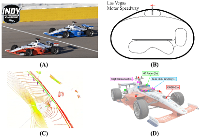
Figure 4: (A) Data from overtaking competition, LVMS CES 2024. (B) LVMS track layout. (C) LiDAR point cloud data. (D) AV-21 sensor setup.

This section outlines the experimental setup and validation results for the DKMGP-integrated E-kin model, focusing on its prediction accuracy and real-time performance.

5.1 Real-world Data Collection

We evaluate the performance of the DKMGP model using real-world autonomous racing data collected from AV-21, a full-scale, fully autonomous racecar that competes in the Indy Autonomous Challenge (IAC). AV-21 is equipped with LiDAR, GNSS, cameras, radar, and advanced computing hardware essential for autonomous operation, as shown in Fig. 4(D). The data was collected during an autonomous passing competition held at the Las Vegas Motor Speedway (LVMS) during the 2024 IAC CES event, as shown in 4. In this data, our racecar achieved a top speed of $230\text{\,}\mathrm{km}\text{\,}{\mathrm{h}}^{-1}$. State estimations obtained using an EKF algorithm are logged at $100\text{\,}\mathrm{Hz}$ and recorded as ROS2 bag files. These bag files (similar to RACECAR [Kulkarni et al.(2023)Kulkarni, Chrosniak, Ducote, Sauerbeck, Saba, Chirimar, Link, Behl, and Cellina] dataset) are processed to construct the dataset, $D_{real}$.

Hyperparameters	Range ; Optimal Values
Batch Size	80 to 280 ; 144
Epochs	400 to 1300 ; 1140
Kernel Functions	SM, RQ, RBF, Polynomial, Periodic, Matérn; RBF
Hidden Layer 1 Size	128 to 512 neurons; 256
Hidden Layer 2 Size	32 to 64 neurons; 64
Learning Rate	0.005 to 0.1; 0.0064
Number of Features	3 to 5; 5

Table 2: Hyperparameter Ranges and Optimal Values

This data is split into a training set and a testing set. The training set contains data from approximately 17 laps ($1410\text{\,}\sec$), while the testing set, which remains unseen by the model, consists of data from a different set of another 17 laps ($1417\text{\,}\sec$).

5.2 DKMGP Hyperparameters Tuning

We performed extensive hyperparameter tuning and ablation study for the DKMGP Model, optimizing parameters such as batch size, epoch count, kernel type, DNN hidden layer sizes, learning rate, and the number of features from the DKL feature extractor. Using the Optuna API ([Akiba et al.(2019)Akiba, Sano, Yanase, Ohta, and Koyama]), we conducted 400 trials on an NVIDIA GeForce RTX 3080 GPU, with 32 GB RAM and an Intel Core i7 processor. Weights & Biases ([Biewald(2020)]) tracked the hyperparameter configurations and metrics for analysis. The ranges and optimal values for each hyperparameter are presented in detail in Table 2.

5.3 DKMGP Model Validation

Fixed Horizon	n3	n5	n10	n15	DKL-SKIP
Inf. Rate	$22.45\text{\,}\mathrm{Hz}$	$35.38\text{\,}\mathrm{Hz}$	$61.35\text{\,}\mathrm{Hz}$	$75.33\text{\,}\mathrm{Hz}$	$0.043\text{\,}\mathrm{Hz}$

Table 3: Inference rates for DKMGPs and DKL-Skip over a 43-step prediction horizon

DKMGP real-time performance We use the same hardware setup described in Section 5.2 to evaluate the DKMGP model efficiency. Additionally, we implement the DKL-SKIP approach under identical conditions to provide a comparison with the proposed DKMGP method. As shown in Table 3, the inference rate of the DKMGP models, without code optimization, achieves inference rates between $22.45\text{\,}\mathrm{Hz}$ (n3) and $75.33\text{\,}\mathrm{Hz}$ (n15), which are approximately 522 to 1752 times faster than the DKL-SKIP rate of $0.043\text{\,}\mathrm{Hz}$, over a total 43-step prediction horizon. The inefficiency of DKL-SKIP arises from its use of three separate GP models to correct for each error term, $\{\epsilon_{v_{x}},\epsilon_{v_{y}},\epsilon_{\omega}\}$, individually, combined with its single-step prediction approach. In contrast, the DKMGP model simultaneously predicts all error terms over multiple steps, leading to a more efficient inference process. Consequently, these results demonstrate that the DKMGP model offers a significant enhancement over DKL-SKIP in real-time performance for vehicle dynamics modeling.

Step	Metric	Error Type
		$\mu_{v_{x}}$	$\mu_{v_{y}}$	$\mu_{\omega}$
DKL-SKIP	MAE	0.1311	0.0533	0.0218
	RMSE	0.2341	0.0835	0.0315
DKMGP	MAE	0.1351	0.0943	0.0424
	RMSE	0.2300	0.1272	0.0547
E-kin ST	MAE	0.2521	1.0084	0.5868
	RMSE	0.3059	1.6511	0.9708

Table 4: Comparison of prediction errors across different models.

Figure 5: Comparison of DKMGP models across different fixed correction horizons.

DKMGP prediction accuracy We first compare the ACH-based DKMGP model to DKMGP models with fixed-length correction horizons. Figure 5 shows prediction results across a 43-step horizon ($1.7\text{\,}\sec$), specifically assessing cross-track errors (CTE) by comparing model predictions to ground truth. The ACH-based DKMGP consistently achieves the smallest CTE, aligning closely with ground truth measurements. Additionally, the DKMGP model’s predictions remain within half a car length, minimizing the risk of track boundary collisions. Then, we compare the prediction accuracy of DKMGP to the DKL-SKIP method-based E-kin model, all benchmarked against an uncorrected E-kin model using mean absolute error (MAE) and root mean squared error (RMSE) as metrics. The inference rate of DKL-SKIP ($0.043\text{\,}\mathrm{H}\mathrm{z}$) was too slow to evaluate its performance on the entire dataset, and therefore, its validation was restricted to just a single lap from the data with average values of base states being $v_{x}=$54.5\text{\,}\mathrm{m}\text{\,}{\mathrm{s}}^{-1}$$, $v_{y}=$0.31\text{\,}\mathrm{m}\text{\,}{\mathrm{s}}^{-1}$$, and $\omega=$0.19\text{\,}\mathrm{rad}\text{\,}{\mathrm{s}}^{-1}$$. As shown in Table 4, the DKL-SKIP achieves slightly higher accuracy than the DKMGP model, with relative errors lower by 0.07%, 13.23%, and 10.79% of the averages for $v_{x}$, $v_{y}$, and $\omega$, respectively. However, this minor accuracy gain comes with a significant trade-off in computational efficiency as due to DKL-SKIP’s low inference rate. Notably, DKMGP demonstrates substantial improvements over the uncorrected E-Kin model, especially with relative errors in $v_{y}$, and $\omega$ that are 294.19%, and 286.32% lower, respectively.

5.4 Comparison of DKMGP and Nonlinear Singe-track

Finally, we compare the DKMGP-based E-kin model with a nonlinear single-track model, which has been validated as effective for modeling vehicle dynamics at high speeds exceeding $230\text{\,}\mathrm{km}\text{\,}{\mathrm{h}}^{-1}$ in autonomous racing. Developing this model required years of data collection and extensive parameter tuning across subsystems, including tuning tire and drivetrain parameters using manufacturer-provided data, and dyno testing (expensive). We compare DKMGP with this well-tuned physics-based model to evaluate its accuracy, acknowledging that such a model would be challenging to obtain in practice. We use sectional average cross-track error (sCTE) as the metric, with each section covering a 2-second interval. This segmentation allows for detailed analysis of prediction accuracy across track sections while minimizing the impact of short-term outliers. Figure 6 shows the sCTE comparison between the DKMGP-based E-kin model (red) and the single-track model (blue).

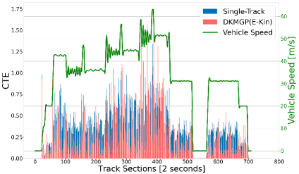
Figure 6: Comparison of sectional cross-track errors between the single-track model and the DKMGP (E-kin) model.

The E-kin model consistently achieves lower sCTE below $40\text{\,}\mathrm{m}\text{\,}{\mathrm{s}}^{-1}$, showing better prediction performance over the single-track model under these conditions. This advantage indicates that the E-kin model’s adaptive correction capabilities allow it to closely follow ground truth measurements. At higher speeds above $45\text{\,}\mathrm{m}\text{\,}{\mathrm{s}}^{-1}$, the single-track model excels due to its ability to account for slip angle effects in vehicle dynamics. Notably, the E-kin model is still able to maintain accuracy within one car width from ground truth, which is within the margin of safety typically used in autonomous racing. These findings demonstrate that with significantly lower effort in model building and tuning, the E-kin model, together with DKMGP, can outperform the single-track model at low to moderate speeds while achieving comparable performance at higher speeds.

6 Conclusions

In this paper, we developed a DKMGP-based E-kin model to capture the dynamics of a full-size autonomous racecar. The DKMGP model overcomes the limitations of existing methods by predicting all state residuals using a single model. Additionally, we present an adaptive correction horizon algorithm that enables DKMGP for multi-step prediction. Evaluation with real-world data from the Indy Autonomous Challenge showed that DKMGP achieves comparable accuracy to DKL-SKIP, while providing orders of magnitude higher computational efficiency than DKL-SKIP, with inference rates $\sim 500$ to 1700 times faster, making it suitable for model-based predictive control. Above all, the DKMGP combined with E-kin model, requires significantly less development effort, compared to a nonlinear single-track model. Future work will focus on implementing and evaluating DKMGP within a closed-loop controller, such as model predictive control, and incorporating the uncertainty provided by GP models to improve controller performance and safety.

Supplementary Demo Video

A demo reel showcasing the Deep Kernel-based Multi-task Gaussian Process (DKMGP) in action, including real-time vehicle dynamics prediction and its application in high-speed autonomous racing, is available at https://youtu.be/q6qFsDyoGqQ

References

- [Akiba et al.(2019)Akiba, Sano, Yanase, Ohta, and Koyama] Takuya Akiba, Shotaro Sano, Toshihiko Yanase, Takeru Ohta, and Masanori Koyama. Optuna: A next-generation hyperparameter optimization framework. In Proceedings of the 25th ACM SIGKDD international conference on knowledge discovery & data mining, pages 2623–2631, 2019.
- [Althoff et al.(2017)Althoff, Koschi, and Manzinger] Matthias Althoff, Markus Koschi, and Stefanie Manzinger. Commonroad: Composable benchmarks for motion planning on roads. In 2017 IEEE Intelligent Vehicles Symposium (IV), pages 719–726. IEEE, 2017.
- [Alvarez et al.(2012)Alvarez, Rosasco, Lawrence, et al.] Mauricio A Alvarez, Lorenzo Rosasco, Neil D Lawrence, et al. Kernels for vector-valued functions: A review. Foundations and Trends® in Machine Learning, 4(3):195–266, 2012.
- [Babu and Behl(2020)] Varundev Suresh Babu and Madhur Behl. f1tenth. dev-an open-source ros based f1/10 autonomous racing simulator. In 2020 IEEE 16th International Conference on Automation Science and Engineering (CASE), pages 1614–1620. IEEE, 2020.
- [Betz et al.(2022)Betz, Zheng, Liniger, Rosolia, Karle, Behl, Krovi, and Mangharam] Johannes Betz, Hongrui Zheng, Alexander Liniger, Ugo Rosolia, Phillip Karle, Madhur Behl, Venkat Krovi, and Rahul Mangharam. Autonomous vehicles on the edge: A survey on autonomous vehicle racing. IEEE Open Journal of Intelligent Transportation Systems, 3:458–488, 2022.
- [Biewald(2020)] Lukas Biewald. Experiment tracking with weights and biases, 2020. URL https://www.wandb.com/. Software available from wandb.com.
- [Carrau et al.(2016)Carrau, Liniger, Zhang, and Lygeros] Jesús Velasco Carrau, Alexander Liniger, Xiaojing Zhang, and John Lygeros. Efficient implementation of randomized mpc for miniature race cars. In 2016 European Control Conference (ECC), pages 957–962. IEEE, 2016.
- [Chrosniak et al.(2024)Chrosniak, Ning, and Behl] John Chrosniak, Jingyun Ning, and Madhur Behl. Deep dynamics: Vehicle dynamics modeling with a physics-constrained neural network for autonomous racing. IEEE Robotics and Automation Letters, 2024.
- [Da Lio et al.(2020)Da Lio, Bortoluzzi, and Rosati Papini] Mauro Da Lio, Daniele Bortoluzzi, and Gastone Pietro Rosati Papini. Modelling longitudinal vehicle dynamics with neural networks. Vehicle System Dynamics, 58(11):1675–1693, 2020.
- [Hartmann et al.(2021)Hartmann, Shiller, and Azaria] Gabriel Hartmann, Zvi Shiller, and Amos Azaria. Autonomous head-to-head racing in the indy autonomous challenge simulation race. arXiv preprint arXiv:2109.05455, 2021.
- [Hermansdorfer et al.(2020)Hermansdorfer, Trauth, Betz, and Lienkamp] Leonhard Hermansdorfer, Rainer Trauth, Johannes Betz, and Markus Lienkamp. End-to-end neural network for vehicle dynamics modeling. In 2020 6th IEEE Congress on Information Science and Technology (CiSt), pages 407–412, 2020. 10.1109/CiSt49399.2021.9357196.
- [Jain et al.(2021)Jain, O’Kelly, Chaudhari, and Morari] Achin Jain, Matthew O’Kelly, Pratik Chaudhari, and Manfred Morari. Bayesrace: Learning to race autonomously using prior experience. In Conference on Robot Learning, pages 1918–1929. PMLR, 2021.
- [Kabzan et al.(2019)Kabzan, Hewing, Liniger, and Zeilinger] Juraj Kabzan, Lukas Hewing, Alexander Liniger, and Melanie N Zeilinger. Learning-based model predictive control for autonomous racing. IEEE Robotics and Automation Letters, 4(4):3363–3370, 2019.
- [Kulkarni et al.(2023)Kulkarni, Chrosniak, Ducote, Sauerbeck, Saba, Chirimar, Link, Behl, and Cellina] Amar Kulkarni, John Chrosniak, Emory Ducote, Florian Sauerbeck, Andrew Saba, Utkarsh Chirimar, John Link, Madhur Behl, and Marcello Cellina. Racecar-the dataset for high-speed autonomous racing. In 2023 IEEE/RSJ International Conference on Intelligent Robots and Systems (IROS), pages 11458–11463. IEEE, 2023.
- [Liniger et al.(2015)Liniger, Domahidi, and Morari] Alexander Liniger, Alexander Domahidi, and Manfred Morari. Optimization-based autonomous racing of 1: 43 scale rc cars. Optimal Control Applications and Methods, 36(5):628–647, 2015.
- [Ning and Behl(2023a)] Jingyun Ning and Madhur Behl. Scalable deep kernel gaussian process for vehicle dynamics in autonomous racing. In Conference on Robot Learning, pages 761–773. PMLR, 2023a.
- [Ning and Behl(2023b)] Jingyun Ning and Madhur Behl. Vehicle dynamics modeling for autonomous racing using gaussian processes. arXiv preprint arXiv:2306.03405, 2023b.
- [Ning and Behl(2024)] Jingyun Ning and Madhur Behl. Gaussian processes for vehicle dynamics learning in autonomous racing. SAE International Journal of Vehicle Dynamics, Stability, and NVH, 8(10-08-03-0019), 2024.
- [O’Kelly et al.(2019)O’Kelly, Sukhil, Abbas, Harkins, Kao, Pant, Mangharam, Agarwal, Behl, Burgio, et al.] Matthew O’Kelly, Varundev Sukhil, Houssam Abbas, Jack Harkins, Chris Kao, Yash Vardhan Pant, Rahul Mangharam, Dipshil Agarwal, Madhur Behl, Paolo Burgio, et al. F1/10: An open-source autonomous cyber-physical platform. arXiv preprint arXiv:1901.08567, 2019.
- [Pacejka(2005)] Hans Pacejka. Tire and vehicle dynamics. Elsevier, 2005.
- [Pan et al.(2021)Pan, Nie, Li, and Gu] Yongjun Pan, Xiaobo Nie, Zhixiong Li, and Shuitao Gu. Data-driven vehicle modeling of longitudinal dynamics based on a multibody model and deep neural networks. Measurement, 180:109541, 2021.
- [Raji et al.(2022)Raji, Liniger, Giove, Toschi, Musiu, Morra, Verucchi, Caporale, and Bertogna] Ayoub Raji, Alexander Liniger, Andrea Giove, Alessandro Toschi, Nicola Musiu, Daniele Morra, Micaela Verucchi, Danilo Caporale, and Marko Bertogna. Motion planning and control for multi vehicle autonomous racing at high speeds. In 2022 IEEE 25th International Conference on Intelligent Transportation Systems (ITSC), pages 2775–2782. IEEE, 2022.
- [Rasmussen(2003)] Carl Edward Rasmussen. Gaussian processes in machine learning. In Summer school on machine learning, pages 63–71. Springer, 2003.
- [Van Niekerk et al.(2017)Van Niekerk, Damianou, and Rosman] Benjamin Van Niekerk, Andreas Damianou, and Benjamin Rosman. Online constrained model-based reinforcement learning. Conf. Uncertainty in Artificial Intelligence, 2017.
- [Wainwright et al.(2008)Wainwright, Jordan, et al.] Martin J Wainwright, Michael I Jordan, et al. Graphical models, exponential families, and variational inference. Foundations and Trends® in Machine Learning, 1(1–2):1–305, 2008.
- [Weiss and Behl(2020)] Trent Weiss and Madhur Behl. Deepracing: Parameterized trajectories for autonomous racing. arXiv preprint arXiv:2005.05178, 2020.
- [Wilson et al.(2016)Wilson, Hu, Salakhutdinov, and Xing] Andrew Gordon Wilson, Zhiting Hu, Ruslan Salakhutdinov, and Eric P Xing. Deep kernel learning. In Artificial intelligence and statistics, pages 370–378. PMLR, 2016.
- [Wischnewski et al.(2022)Wischnewski, Geisslinger, Betz, Betz, Fent, Heilmeier, Hermansdorfer, Herrmann, Huch, Karle, et al.] Alexander Wischnewski, Maximilian Geisslinger, Johannes Betz, Tobias Betz, Felix Fent, Alexander Heilmeier, Leonhard Hermansdorfer, Thomas Herrmann, Sebastian Huch, Phillip Karle, et al. Indy autonomous challenge-autonomous race cars at the handling limits. In 12th International Munich Chassis Symposium 2021: chassis. tech plus, pages 163–182. Springer, 2022.