Interfacial Water Polarization: A Critical Force for Graphene-based Electrochemical Interfaces

Abstract

Water molecules predominantly act as solvents in electrochemical systems and are often modeled as a passive dielectric medium. In this work, we use molecular dynamics simulations and theoretical analysis to revisit this conventional view. We reveal that the interfacial polarized water overscreens the electrostatic potential between ions and the surface beyond being a passive dielectric medium. This overscreening enables the interfacial water to dominate the electric potential spatial distribution, inverting the electrode surface potential polarity and dominating the capacitance. A model is then developed to incorporate this critical interfacial water polarization.

Aqueous electrolytes in contact with conductive solid materials are fundamental to numerous technologies related to energy, water, and biomedicine. Fundamental to the electrochemical interface is the formation of an electric double layer (EDL), where nearby liquid ions and water dipoles balance surface charges or mismatched work functions, leading to spatially reorganized electric and chemical potentials [1]. Numerous studies have shown that EDL-mediated potentials are crucial for various electrochemical and biological processes, including ionic pumps, charge storage, electrode stability, electrolyte conductivity, and electrochemical reaction kinetics [2, 3, 4, 5, 6]. Under the framework of the Gouy–Chapman–Stern (GCS) model, a foundation of EDL theory, the EDL compromises a near-surface compact layer (called Stern layer) and a diffuse layer behind it. Notably, under the operation of large electrode polarization and medium/high concentration electrolytes ($>$0.1 M), which is common for many practical applications, the Stern layer dominates the electric and chemical potentials, governing the performance and efficiency of these technologies [7, 8]. However, due to its sub-nanometric width and location buried between electrodes and the diffuse layer, the Stern layer has long remained elusive and is usually modeled as an effective physical parallel capacitor in the GCS model.

Recently, the investigations of EDL, particularly on the Stern layer, have seen promising progress on account of new spectroscopy techniques, such as optical-vibrational spectroscopies based on infrared absorption [9] and Raman scattering [10]. These state-of-the-art characterizations allow the possibility of probing the structural and electrical characteristics of ions and solvents within the Stern layer. The reported structural features of water solvent suggest that its impact would be oversimplified within the GCS model, particularly at the Stern layer [7, 8, 11, 12, 13, 14, 15]. For example, based on graphene’s well-defined atomically flat surface and its transparency in the relevant infrared frequency range, the surface-specific vibrational spectroscopy experiments, coupled with molecular simulations, revealed a higher local density of water near the graphene surface than the bulk solution [16, 17]. Additionally, the O–H bond of water in this region exhibits a directional preference pointing towards the graphene [12, 13]. Given that water is a polar solvent, the recognized local density heterogeneity and specific molecular orientation would alter the spatial distribution of electric potentials beyond being a homogeneous medium assumed in the GCS model. Moreover, an asymmetric orientation response of interfacial water between positive and negative electric fields has also been reported [12, 13, 14, 15], suggesting that water would not be a constant dielectric media as a function of electrode polarization. How these heterogeneous interfacial water structures will affect the electric potential spatial distribution across the EDL, particularly within the Stern layer, remains largely unclear.

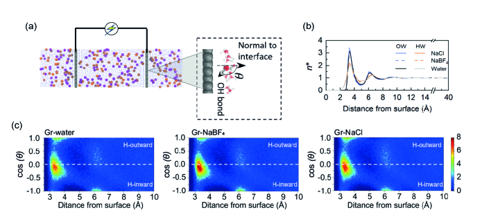
Figure 1: The structured water at the uncharged interface. (a) The representative model system with the water molecules as points, cations as purple spheres, anions as orange spheres, and graphene as grey spheres. (b) Normalized local number distributions of water’s oxygen (OW) and hydrogen (HW) atoms vs. a normal distance to the graphene surface. (c) Normalized orientation density of water’s O–H bond as a normal distance to the graphene surface. The horizontal white line divides the map into bonds pointing away from the surface (termed H-outward) and toward the surface (H-inward).

In this letter, we choose a graphene-interfaced aqueous electrolyte as a model system to scrutinize how interfacial water affects the local electric potential distributions and resultant electrochemical performance [Fig. 1(a)]. Given that the local density and orientation of water dipoles would be altered by the graphene surface, ions, and charging states of graphene, we consider multiple systems to facilitate a controlled investigation, including graphene-interfaced pure water system (Gr-water), graphene-interfaced NaCl aqueous electrolyte system (Gr-NaCl), and graphene-interfaced $\text{NaBF}_{4}$ aqueous electrolyte system (Gr-$\text{NaBF}_{4}$). NaCl is widely taken as the standard aqueous electrolyte. The $\text{BF}^{-}_{4}$ is considered because the interfacial water structure would be more susceptible to its strong non-electrostatic adsorption on the graphene surface [18, 19]. The electrolyte concentration is 0.8 M. Different charging states of graphene (electroneutral, positively charged, and negatively charged) are also investigated. By using molecular dynamics (MD) simulations, we examine the structural distribution of water dipoles and ions as a function of the normal distance from the graphene surface. By incorporating these microscopic structural characteristics into theoretical frameworks, we quantify the contributions of water dipoles and ionic charges to total electric potential distributions. For more simulation details, please see Supplemental Material and our previous work [20]. We reveal that the interfacial polarized water overscreens the electrostatic potential between ions and the surface beyond being a passive dielectric medium. This overscreening enables the interfacial water to dominate the electric potential spatial distribution and can invert the electrode surface potential polarity. An EDL model is developed to incorporate this interfacial water effect.

Crucial interfacial water in the electric potential distributions at uncharged graphene.—Consistent with experimental characterizations [12, 13, 14, 15] and ab initio molecular dynamics results [17], the water shows structural heterogeneities at the near-surface region even if the graphene is uncharged [Fig. 1(b-c)]. A local density peak, approximately 3.5 times greater than that in the bulk region, occurs at a distance of three angstroms from the graphene surface. In this interfacial water, some hydrogen atoms are positioned closer than the oxygen atoms to the graphene surface, consistent with the reported dangling O–H bond of water pointing towards the graphene [12, 13, 14, 15]. This polarized structure is further confirmed by analyzing the water’s orientation [Fig. 1(c)]. We define an orientation angle $\theta$, which represents the direction of the O–H bond relative to the normal plane of the graphene surface [inset in Fig. 1(a)]. The color maps in Fig. 1(c) show that within 5 Å of the surface, most water molecules exhibit negative cos$\theta$ values, corresponding to the O–H bond pointing towards the surface. Notably, this interfacial water polarization remains consistent across Gr-water, Gr-NaCl, and Gr-$\text{NaBF}_{4}$ systems [Fig. 1(b-c)], showing that the presence and specific identity of ions introduce minor alterations.

To elucidate how interfacial water affects the electric potential distributions, we first focus on uncharged conditions. We compare the total electric potential profile of Gr-NaCl or Gr-$\text{NaBF}_{4}$ system ($\phi_{\mathrm{pzc,total}}$) with that of the Gr-water system ($\phi^{0}_{\mathrm{pzc,H2O}}$) [Fig. 2(a-b)]. Interestingly, $\phi_{\mathrm{pzc,total}}$ and $\phi^{0}_{\mathrm{pzc,H2O}}$ show similar local fluctuations and magnitudes . The $\phi_{\mathrm{pzc,total}}$ is nearly zero in the region located 10 Å to 40 Å from the graphene surface. This is consistent with this region’s uniform distribution of cations and anions [lower plot, Fig. 2(a-b)]. However, within 10 Å of the surface, $\phi_{\mathrm{pzc,total}}$ presents profound oscillations, ranging from $-0.75\,\text{V}$ to 0.4 V. Notably, the $\phi^{0}_{\mathrm{pzc,H2O}}$ also show the same oscillations. In the uncharged Gr-water system, the total electric potential $\phi^{0}_{\mathrm{pzc,H2O}}$ arises only from water’s polarizations modulated by the graphene surface. The similarity between $\phi_{\mathrm{pzc,total}}$ and $\phi^{0}_{\mathrm{pzc,H2O}}$ suggests that the interfacial water polarized by the graphene surface may also play a crucial role in the Gr-NaCl and Gr-$\text{NaBF}_{4}$ systems. Note that these non-monotonic potential profiles, which determine the local electric field strength, differ markedly from the linear potential drop predicted by the GCS model.

The crucial impact of interfacial water on electric potential is also supported by another phenomenon: the sign of potential of zero charge (PZC) is inconsistent with the ionic charge polarity at interfacial regions. The Gr-NaCl system shows a PZC of 0.33 V [Fig. 2(a) and Supplemental Materials Sec.4]. However, $\text{Na}^{+}$ and $\text{Cl}^{-}$ ions show a nearly equal local distribution [lower plot, Fig. 2(a)], which would not contribute to such a significant positive PZC value. This phenomenon is striking in the Gr-$\text{NaBF}_{4}$ system; it has a positive PZC of 0.26 V [Fig. 2(b) and Supplemental Materials Sec.4]. This contrasts with the negative charge polarity contributed by the spatial distribution of $\text{NaBF}_{4}$ ions, where the $\text{BF}^{-}_{4}$ ions show a closer adsorption distance and around three times higher local absorption density than $\text{Na}^{+}$ ions at the graphene surface [lower plot, Fig. 2(b)]. Note that the simulated PZC values are close to the reported experimental results [13].

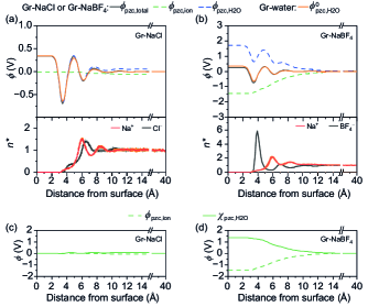
Figure 2: Interfacial water dominates the electrolyte electric potential at the uncharged graphene surface. (a-b) The upper plots are the electric potential profiles, including $\phi_{\mathrm{pzc,total}}$, $\phi_{\mathrm{pzc,ion}}$, and $\phi_{\mathrm{pzc,H2O}}$, in Gr-NaCl system (a) and Gr-$\text{NaBF}_{4}$ system (b). The electric potential profile in the Gr-water system, $\phi^{0}_{\mathrm{pzc,H2O}}$, is also included as a comparison. The lower plots are the normalized local number distributions of ions as a normal distance from the uncharged graphene surface in the Gr-NaCl system (a) and Gr-$\text{NaBF}_{4}$ system (b). (c-d) The electric potential profiles, $\phi_{\mathrm{pzc,ion}}$ and $\chi_{\mathrm{pzc,H2O}}$, in Gr-NaCl system (c) and Gr-$\text{NaBF}_{4}$ system (d).

Interfacial water beyond a passive dielectric medium. —Given that the aforementioned total electric potential profiles $\phi_{\mathrm{pzc,total}}$ are dictated by the distribution of ions and the arrangement of water molecules, we derive the electric potential profiles contributed by ions ($\phi_{\mathrm{pzc,ion}}$) and water ($\phi_{\mathrm{pzc,H2O}}$) by integrating the corresponding spatial charge or polarization distributions for further analysis [details in Supplemental Material Sec.3]. Note that according to the linearity of Maxwell’s equations, the total electric potential is the sum of them: $\phi_{\mathrm{pzc,total}}=\phi_{\mathrm{pzc,ion}}+\phi_{\mathrm{pzc,H2O}}$. Interestingly, in either Gr-NaCl or Gr-$\text{NaBF}_{4}$ system, $\phi_{\mathrm{pzc,H2O}}$ shows a larger magnitude over $\phi_{\mathrm{pzc,ion}}$, particularly at the near-surface region [Fig. 2(a-b)]: showing an overscreen effect. For example, in the Gr-NaCl system, the $\phi_{\mathrm{pzc,ion}}$ is almost flat as a function of normal distance from the graphene surface and its PZC is $-0.01\,\text{V}$. By contrast, the $\phi_{\mathrm{pzc,H2O}}$ shows a non-monotonic profile and its PZC is 0.34 V. In the Gr-$\text{NaBF}_{4}$ system, $\phi_{\mathrm{pzc,ion}}$ shows a negative PZC of $-1.45\,\text{V}$, while the $\phi_{\mathrm{pzc,H2O}}$ shows a PZC of 1.71 V, overriding the magnitude of $\phi_{\mathrm{pzc,ion}}$ and leading to a positive total PZC value.

The larger magnitude of $\phi_{\mathrm{pzc,H2O}}$ over $\phi_{\mathrm{pzc,ion}}$ is inconsistent with the classic dielectric theory for aqueous electrolytes, where water is modelled as a passive dielectric media to attenuate the electrostatic interaction among surface charge and electrolyte ions [21]. This disparity motivates us to dissect the $\phi_{\mathrm{pzc,H2O}}$ in Gr-NaCl and Gr-$\text{NaBF}_{4}$ systems into two components: the water polarization by graphene surface $\phi^{0}_{\mathrm{pzc,H2O}}$ and the residual part $\chi_{\text{H2O}}$, as $\phi_{\mathrm{pzc,H2O}}=\phi^{0}_{\mathrm{pzc,H2O}}+\chi_{\text{H2O}}$. Figure 2 (c-d) shows that the $\chi_{\text{H2O}}$ manifests as a nearly mirror image to $\phi_{\mathrm{pzc,ion}}$ relative to the x-axis, both in localized fluctuations and magnitudes. This phenomenon suggests that $\chi_{\text{H2O}}$ exhibits a linear passive dielectric effect on $\phi_{\mathrm{pzc,ion}}$ as a consequence of the water shielding effects. In other words, the polarization of water due to ions is primarily manifested in $\chi_{\text{H2O}}$. The near compensation between them also reveals that the water polarization by graphene surface ($\phi^{0}_{\mathrm{pzc,H2O}}$) dominates the total electric potential as observed in Fig.2: $\phi_{\mathrm{pzc,total}}=\phi_{\mathrm{pzc,ion}}+\phi^{0}_{\mathrm{pzc,H2O}}+\chi_{\text{H2O}}\approx\phi^{0}_{\mathrm{pzc,H2O}}$.

Given that the classic Poisson-Boltzmann (PB) equation accounts for the water’s linear passive dielectric effect on electrolyte ions (i.e., the effect of $\chi_{\text{H2O}}$ on $\phi_{\mathrm{pzc,ion}}$) but ignores the $\phi^{0}_{\mathrm{pzc,H2O}}$, we therefore modify the Poisson equation via accounting for the $\phi^{0}_{\mathrm{pzc,H2O}}$:

$$\nabla^{2}\phi_{\mathrm{pzc,total}}(z)=\nabla^{2}\left(\phi^{0}_{\mathrm{pzc,H2O}}(z)+\chi_{\text{H2O}}(z)+\phi_{\mathrm{pzc,ion}}(z)\right)$$ (1)

$$\nabla^{2}\left(\phi_{\mathrm{pzc,total}}(z)-\phi^{0}_{\mathrm{pzc,H2O}}(z)\right)=-\frac{\rho_{\mathrm{ion}}(z)}{\varepsilon_{r}\varepsilon_{0}}$$ (2)

where $\varepsilon_{r}$ is the relative dielectric constant; $\varepsilon_{0}$ is the dielectric constant at vacuum. The local ion charge density, $\rho_{\mathrm{ion}}$, is described via a modified Boltzmann equation:

$$\rho_{\mathrm{ion}}(z)=\sum_{i}ez_{i}c_{i}=ec_{i}^{0}\sum_{i}z_{i}e^{-\frac{z_{i}e(\phi_{\mathrm{pzc,total}(z)}-\phi^{0}_{\mathrm{pzc,H2O}}(z))+V_{i}^{\mathrm{PMF}}}{k_{B}T}}$$ (3)

where $c_{i}^{0}$ is the bulk concentration of ion species $i$, $k_{B}$ is the Boltzmann constant, and $T$ is temperature. The $V_{i}^{\mathrm{PMF}}$ represents the non-electrostatic interaction energy between ion $i$ and graphene to account for the ion-specific surface adsorption effect [18]. Eqs. (2) and (3) form our modified PB equation for the uncharged scenario [see more details in Supplemental Material].

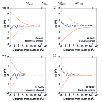
Figure 3: The changes in the electric potential profiles at charged graphene surfaces relative to the uncharged condition. (a) and (b) compare the Gr-NaCl system with the Gr-water system: at a negatively charged surface (a) and at a positively charged surface (b). (c) and (d) compare the Gr-$\mathrm{NaBF}_{4}$ system with the Gr-water system: at the negatively charged surface (c) and the positively charged surface (d). In each scenario, the sub-components of $\Delta\phi_{\mathrm{total}}$ ($\Delta\phi_{\mathrm{ion}}$ and $\Delta\chi_{\mathrm{H2O}}$), are computed. The charge densities, $\sigma_{s}=\pm 0.00938\,\text{e C-atom}^{-1}\,(6.0\,\mu\text{C cm}^{-2})$, are adopted to model the charged graphene sheet.

The impact of interfacial water in charged scenarios and advanced EDL model.—The influence of interfacial water at charged graphene is evaluated by analyzing the changes in electric potential profiles relative to uncharged conditions. All symbols in the following adorned with the prefix “$\Delta$” denote such changes in potential profiles. For example, $\Delta\phi_{\mathrm{total}}$ represents the change of overall potential, $\Delta\phi_{\mathrm{total}}=\phi_{\mathrm{ele,total}}-\phi_{\mathrm{pzc,total}}$. In Gr-NaCl and Gr-NaBF4 systems, it consists of three components, with $\Delta\phi_{\mathrm{total}}=\Delta\phi^{0}_{\mathrm{H2O}}+\Delta\chi_{\text{H2O}}+\Delta\phi_{\text{ion}}$. Fig. 3(a-d) show that the $\Delta\phi_{\mathrm{total}}$ is predominantly shaped by $\Delta\phi^{0}_{\mathrm{H2O}}$ (the potential changes in Gr-water system). Consistently, the water molecules in these systems show similar structural characteristics [Supplemental Material Sec.5]. This is further corroborated by the calculated capacitances in these systems, which are comparable to those of the Gr-water system [Supplemental Material Sec.6]. The $\Delta\phi_{\mathrm{ion}}$ and $\Delta\chi_{\text{H2O}}$ still compensate each other in a typical dielectric manner.

The response of polarized water, $\Delta\phi^{0}_{\mathrm{H2O}}$, is then considered to describe the electric potentials at charged surfaces:

$$\nabla^{2}\phi_{\mathrm{ele,total}}(z)=\nabla^{2}(\phi_{\mathrm{pzc,total}}(z)+\Delta\phi_{\mathrm{total}}(z))$$ (4)

$$\nabla^{2}(\phi_{\text{ele,total}}(z)-\phi_{\text{pzc,total}}(z))$$

$$=\nabla^{2}\left(\Delta\phi_{\text{ion}}(z)+\Delta\chi_{\text{H2O}}(z)+\Delta\phi_{\text{H2O}}^{0}(z)\right)$$

$$=\nabla^{2}\left(\Delta\phi_{\text{ion}}(z)+\Delta\chi_{\text{H2O}}(z)+\Delta\phi_{\text{H2O,I}}^{0}(z)+\Delta\phi_{\text{H2O,II}}^{0}(z)\right)$$ (5)

Here we split: $\Delta\phi^{0}_{\mathrm{H2O}}(z)=\Delta\phi^{0}_{\mathrm{H2O,I}}(z)+\Delta\phi^{0}_{\mathrm{H2O,II}}(z)$, where the $\Delta\phi^{0}_{\mathrm{H2O,I}}(z)$ represents the linear dielectric response of water in the whole region and $\Delta\phi^{0}_{\mathrm{H2O,II}}(z)$ represents the water’s response at the interfacial region [details see Supplemental Material Sec.7]. We then follow the Poisson equation to obtain:

$$\nabla^{2}(\phi_{\mathrm{ele,total}}(z)-\phi_{\mathrm{pzc,total}}(z)-\Delta\phi^{0}_{\mathrm{H2O,II}}(z))=-\frac{\rho_{\mathrm{ion}}(z)}{\varepsilon_{r}\varepsilon_{0}}$$

The local ion charge density $\rho_{\mathrm{ion}}(z)$ is described via the modified Boltzmann equation:

$$\rho_{\mathrm{ion}}(z) = ec_{i}^{0}\sum_{i}z_{i}e^{-\frac{z_{i}e(\phi_{\mathrm{ele,total}}(z)-\phi_{\mathrm{pzc,total}}(z)-\Delta\phi^{0}_{\mathrm{H2O,II}}(z))+V_{i}^{\mathrm{PMF}}}{k_{B}T}}$$ (7)

Eqs. (6) and (7) form the modified PB equation to describe the electric potentials in charged scenarios.

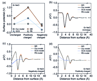
Figure 4: Comparison of theoretical model results in the Gr-NaCl system. (a) The surface potentials predicted by different models, compared with the MD results. (b-d) The electric potential profiles predicted by different models, compared with the MD results. Graphene surfaces are uncharged (a), negatively charged (b), and positively charged (c), respectively.

Figure 4 and Supplemental Material Sec.8-9 show that the developed EDL model improves the prediction of the local electric potential distributions, compared to the classic PB equation (without Stern layer) and the GCS model. This underscores the critical contribution of interfacial water polarization modulated by the graphene surface (i.e., $\phi^{0}_{\mathrm{pzc,H2O}}$ at the uncharged surface and $\Delta\phi^{0}_{\mathrm{H2O}}$ at the charged surfaces). The quantitative comparison of the surface potential values further confirms this. Take the Gr-NaCl system as an example [Fig. 4]. PB and GCS predict the PZC to be 0 V, while the developed model predicts the PZC to be 0.34 V, close to the MD result of 0.33 V. Additionally, the developed model predicts 0.99 V at the positively charged surface and $-0.10\,\text{V}$ at the negatively charged surface, closely matching MD results of 0.98 V and $-0.12\,\text{V}$, respectively. In contrast, the PB equation, which adopts a uniform dielectric constant across the whole solution region, predicts only 0.01 V and $-0.01\,\text{V}$, respectively [Fig. 4(a)]. It is one magnitude smaller than the MD results. Compared to the classic PB equation, the GCS model shows some improvements in the surface potential prediction (0.35 V and $-0.35\,\text{V}$, respectively), though significant quantitative differences still remain. Additionally, it fails to capture the asymmetric surface potentials between positively and negatively charged surfaces, and its linear-decayed local electric potential within the Stern layer deviates from the expected non-monotonic profiles. For ion density distribution profiles, our models also show good consistency with MD simulation results [Supplemental Material Sec.9]. The same improvement is also shown in the Gr-$\text{NaBF}_{4}$ system [Supplemental Material Sec.8].

Summary.—In this work, via utilizing MD simulations and theoretical analysis, we unravel how interfacial water molecules at the graphene surface contribute to the spatial distribution of electric potentials in the system. Beyond the traditional assumptions of water as a passive dielectric medium, as involved in classic electric double theories, such as the PB equation and GCS model, we reveal that the interfacial water layer overscreens the electrostatic interaction between ions and electrode, contributing an electric potential with a greater magnitude than that from ion charges. It dominates the electric potential distributions in aqueous electrolytes and can even change the polarity of surface potentials, opposite to the charge polarity by ions’ interfacial adsorptions. We reveal that this intriguing overscreening phenomenon originates from interfacial water’s polarized orientation and heterogeneous spatial distribution due to the presence of a graphene surface. Moreover, we develop a modern EDL model, exhibiting improved capability in describing local electric potential profiles and ion spatial distributions at both uncharged and charged graphene surfaces. This advancement enables improved physics-based predictions on multiple electrochemical metrics, such as the PZC values, surface potentials, EDL capacitances, as well as the local electric field strength, which are crucial for the performance engineering of various technical applications, including nanoionics, iontronics, electrochemical energy storage and conversion, and neuromorphic functions.