Competitive binding of Activator-Repressor in Stochastic Gene Expression

Abstract

Regulation of gene expression is the consequence of interactions between the promoter of the gene and the transcription factors (TFs). In this paper, we explore the features of a genetic network where the TFs (activators and repressors) bind the promoter in a competitive way. We develop an analytical theory that offers detailed reaction kinetics of the competitive activator-repressor system which could be the powerful tools for extensive study and analysis of the genetic circuit in future research. Moreover, the theoretical approach helps us to find a most probable set of parameter values which was unavailable in experiments. We study the noisy behaviour of the circuit and compare the profile with the network where the activator and repressor bind the promoter non-competitively. We further notice that, due to the effect of transcriptional reinitiation in the presence of the activator and repressor molecules, there exits some anomalous characteristic features in the mean expressions and noise profiles. We find that, in presence of the reinitiation the noise in transcriptional level remains low while it is higher in translational level than the noise when the reinitiation is absent. In addition, it is possible to reduce the noise further below the Poissonian level in competitive circuit than the non-competitive one with the help of some noise reducing parameters.

^#Department of Science, Digsui Sadhana Banga Vidyalaya, Digsui, Magra, Hooghly-712234, India.

Introduction

For the last two decades, by employing several experiments, it has been widely verified and accepted that the gene expression regulation is a stochastic process [1, 2, 3, 4, 5, 6, 7, 8, 9, 10, 11]. In parallel with the experiments, many theoretical approaches, especially analytical analyses and numerical simulations have built up in support [12, 13, 14, 15, 16, 17, 18, 19, 20, 21, 22]. Regulation of gene expression (GE) is essential for all organisms to develop their ability to respond to environmental changes. It involves several complex stochastic mechanisms such as transcription, preinitiation, reinitiation, translation and degradation, etc. [23, 24]. Transcription is the initial step through which the biological information is being transferred from the genome to the proteome [25]. The regulation of transcription [18, 19] occurs whenever some regulatory proteins called transcription factors (TFs) interact with the promoter of a gene. Based on functionality, TFs are classified as activators and repressors in both prokaryotes and eukaryotes [25, 26, 27]. Repressors inhibit the gene transcription by binding to specific DNA sequences. Tryptophan and Lac are some widely known repressors for prokaryotic systems. On the other hand, activators allow RNA-Polymerase (RNAP) to bind with the promoter and to initiate the transcription resulting in synthesizing mRNA. The molecular concentrations of these activators and/or repressors can be varied with the help of some inducer molecules, such as doxycycline (dox), galactose (GAL), tetracycline (Tc) and anhydrotetracycline (aTc), etc. [3, 10, 11].

An eukaryotic system is much more complex and possesses a compact chromatin structure than prokaryotes. In the eukaryotic system, a basic example of transcriptional regulation by TFs is a two-state telegraphic model [14, 15, 17], where a gene can be either in any of the two states: active (ON) or inactive (OFF) depending on whether TFs are bound to the gene or not. An active gene transcribes through the production of messenger-RNA (mRNA) in a pulsatile fashion during short intense periods known as transcriptional bursts, followed by a longer period of inactivity. This burst mechanism is the source of cellular heterogeneity and stochastic noise [7, 15, 16]. Another crucial mechanism of transcription known as reinitiation [3, 28] is the cause of heterogeneity. This fact has been proved by experiments [3, 6, 9, 29, 30, 31] and recent theories [32, 33, 34].

Although most of the theories describe GE models using numerical simulations, discrete stochastic models like the Gillespie algorithm [35] and continuous stochastic models involving the chemical Langevin equation (CLE) [36]. The use of the Gillespie algorithm and CLE are limited as they require details of the biochemical reaction kinetics and rate parameters which are often unavailable in the performed biological experiments. Due to these limitations, many biological systems remain unmodeled or modelled without stochastic simulations. One such experiment, carried out by Rossi et al. [37] was not modelled. The authors used a dox-controlled synthetic transcription unit driven by activator only, repressor only, or both in an overlapping promoter region. They proposed that the dose-response curve follows the Hill function and the Hill coefficients from the dose-response curves are observed as: 1.6 in the presence of the activator only, 1.8 in the presence of the repressor only and 3.2 when both the activator and repressor operating together exclusively. Rossi et al. suggested that either addition or multiplication of the Hill coefficients 1.6 and 1.8 gives 3.4 and 2.88 ($\approx$2.9) respectively, which differs from what they found to be 3.2. Almost a decade later, Yang and Ko [38] proposed a stochastic Markov chain model (MCM) with a three-state activator-repressor system to explain the deviation of observed Hill coefficients from the expected values.

However, both these approaches were unable to explain the collective (Hill coefficient) and stochastic behavior of the three-state competitive activator-repressor system due to the lack of detailed kinetic rates and parameter values. It is thus desirable to explain the model with a proper theory supported by analytical and/or simulation methods. Accordingly, we develop a theory that offers detailed chemical kinetics of the competitive activator-repressor system and a most probable set of parameter values that were due for decades. The availability of suitable analytical theory and details of reaction kinetics therefore could be the powerful tools for future research and analysis of the genetic networks.

In this paper, we consider the competitive binding of TFs (activators and repressors) to the promoter of the gene. We will explore a two-state activator and/or repressor system first. Next, we will discuss a three-state genetic model where both activator and repressor molecules competitively bind to the promoter. There is evidence that activators and repressors can regulate the transcription by binding the promoter of a gene mutually exclusively [37]. Rossi et al. [37], Biggar and Crabtree [11] have shown experimentally, Yang et al. [38] and Karmakar [16] have shown analytically that the competition between activator and repressor molecules to occupy the promoter region can generate a binary response in gene expression. If the activator or repressor molecules act independently, a graded response is obtained. However, there is no noise profile available for the transcriptional regulation by activators and repressors mutually exclusively in the above-mentioned works. Although, a few studies have explored how the competitive binding of TFs in different scenarios influences gene expression noise [39, 40, 41], nonetheless a general theoretical framework of noisy behaviour of a three-state activator-repressor system still remains unexplored or may stick around in its infancy. Here, we emphasize on studying the noisy behavior of the model and compare its characteristics with a non-competitive activator-repressor model [42]. We will also check the behavior of the architecture in presence of different activator and repressor molecule instead of doxycycline only.

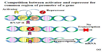
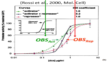
Figure 1: (a)Competition between activator and repressor molecules to bind to a common binding site of promoter of gene (b) Rossi et al. [37] experimental plot: promoter activity fitted with the Hill function.

Activator-repressor system

Regulation of gene expression is the consequence of interactions between the promoter of gene and the transcription factors (TFs). Based on their functionality, TFs are classified as activators and repressors [25, 26, 27]. The activator and repressor molecules can attach to the promoter of gene and proceed their operation in two ways: either competitively [16] or non-competitively [42]. In recent work, Das AK [42] has rigorously discussed the architecture and the noise profile of the non-competitive binding by activator and repressor. In this paper, we will discuss the genetic circuits operated by either activator only or repressor only or by both mutually exclusively. Rossi et al. experimentally [37] showed the dose (dox)-response (green fluorescent protein/GFP) of an activator-repressor system and fitted the parameters with the Hill function. Later, Yang and Ko [38] using stochastic simulation tried to explain the mismatch of the Hill coefficient with the observed experimental data. Furthermore, Karmakar [16] calculates PDF of a three-state stochastic activator-repressor network and explains the transformation of graded to binary response of PDF as observed in the experiment of Rossi et al. [37]. However, except Karmakar [16], the other works did not provide the details of the kinetics and parameters of the system but there is a lack of exact parameter values that are involved in the network. To find the parameter values we use a two-state and a three-state genetic network operated by doxycycline as activator and/or repressor. Although, the aforementioned works use networks that show protein synthesis directly from genes and skipped the intermediate transcription stages (mRNA production). Here, we show all the possible transitions and parameters involved in the system. However, to fit the parameters with the experimental data, we use mRNA dynamics instead of protein (one can consider the transcriptional and translational stages have merged to a single stage, since it is well known that dynamics followed by mRNA reflects exactly to the protein just gets multiplied by a scale factor to the magnitudes [33, 34]), as it reduces the number of parameters and their mathematical complexities.

Generally, activator molecules get attached to the promoter of a gene at a specified region called the activator-binding site (see fig. 1a) and then allow RNAP-II to bind with it to make the gene ready (active/ON) for transcription. On the other hand, when the repressor molecule occupies its binding site, immediately it blocks RNAP-II from sitting on the promoter and the gene goes to the inactive/OFF state i.e. inhibits transcription. In this study, we observe some interesting dynamical behavior (stochasticity and noise) when both activator and repressor compete mutually for a common binding region of the promoter. Furthermore, we compare the characteristic differences between this competitive model with a non-competitive one [42]. In a non-competitive architecture there may be four possible genetic states instead of three, viz. normal state $(G_{n}),$active state $(G_{a}),$ active-repressed state $(G_{ar})$ and repressed state $(G_{r})$ (see fig.9a).

1 Two-state model when only activator is present

We start with a two-state model [14, 15, 17] (fig.2a) where mRNA may produce spontaneously from a normal state of gene $G_{n}$ with a leaky basal rate (very low) $J_{0}$. The gene can be activated by some inducer (activator) like doxycycline (Dox) or galactose (GAL) or by some protein produced by itself (positive feedback). The mRNAs are being produced from the active state $G_{a}$ (ON) at a rate $J_{m}=J_{1}.$ This mechanism of producing mRNA is called transcription. Protein synthesis starts from the new born mRNAs via rate constant $J_{p}$ by the process, commonly known as translation. Both mRNAs and proteins degrade by rates $k_{m}$ and $k_{p}$ respectively.

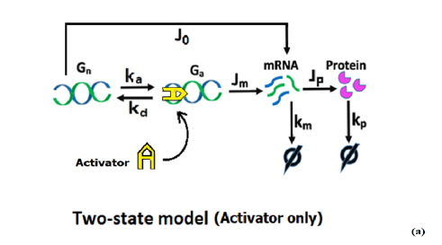
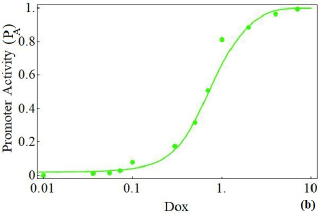
Figure 2: (a) Two-state system where only activator is operating (b) Dose-response curve (solid curve) fitted with experimental data (solid circles) in presence of activator only (repressor absent) in the promoter of gene.

1.1 Model analysis: determination of promoter activity

The time evolution of mRNA concentration can be expressed deterministically as,

$$\frac{dz}{dt}=\frac{J_{i}}{z_{max}}G-k_{m}z=f(z,G)$$ (1)

where $i=0$ (OFF) or =1 (ON) such that $G=0$ (gene is inactive) and G = 1 (gene is active) respectively. The variable $z$ denotes the mRNA concentration at time t normalized by the maximum possible mRNA concentration ($z_{max})$. Only stochasticity is involved as we assume in the transition of promoter to ON and OFF states.

The probability distribution function (PDF) can be written in form of the Fokker-Plank equation as,

$$\frac{\partial P_{i}(z,t)}{\partial t}=-\frac{\partial}{\partial z}[f(z,G)P_{i}(z,t)]+\sum_{j\neq l}{\displaystyle k_{jl}P_{j}(z,t)-k_{lj}P_{j}(z,t)}$$ (2)

The 1st term in RHS is transport term, 2nd one is the gain term and last one implies loss term.

using eq.1 and eq.2 the Champman-Kolmorgov equation for the reaction scheme of fig. (2) can be written as,

$$\frac{\partial P_{0}(z,t)}{\partial t}=-\frac{\partial}{\partial z}[(\frac{J_{0}}{z_{max}}-k_{m}z)P_{0}(z,t)]+k_{d}P_{1}(z,t)-k_{a}P_{0}(z,t)$$ (3)

$$\frac{\partial P_{1}(z,t)}{\partial t}=-\frac{\partial}{\partial z}[(\frac{J_{1}}{z_{max}}-k_{m}z)P_{1}(z,t)]+k_{a}P_{0}(z,t)-k_{d}P_{1}(z,t)$$ (4)

we have continuity equation

$$\frac{\partial P}{\partial t}=-\nabla.\mathscr{\mathcal{J}}$$ (5)

using no flux boundary condition we get the probability current density, $\mathcal{J}=[\frac{J_{i}}{z_{max}}-k_{m}z]P_{i}=0$ and by the steady state condition, $P(z)=P_{1}(z)+P_{0}(z)$ we have the solution of the form

$$P(z)=C_{1}(z-\frac{J_{0}}{k_{m}z_{max}})^{\frac{k_{a}}{k_{m}}-1}(\frac{J_{1}}{k_{m}z_{max}}-z)^{\frac{k_{d}}{k_{m}}-1}$$ (6)

where, $z_{max}=\frac{J_{1}k_{a}+J_{0}k_{d}}{(k_{a}+k_{d})k_{m}}=$ steady state mean mRNA

The normalization constant $C_{1}$ can be obtained by integrating $P(z)$ from $z_{min}=\frac{J_{0}}{k_{m}}$ to $z_{max}$.

Now the steady state probability of finding a cell with $z$, greater than a threshold value $Z_{th}$ is given by

$$P(z >Z_{th})=1-\frac{\intop_{z_{min}}^{Z_{th}}P(z)\ dz}{\intop_{0}^{1}P(z)\ dz}=P_{A}\thinspace(say)$$ (7)

$$or,\quad P_{A}= 1-\frac{\left(Z_{\text{th}}-J_{0}\right){}^{k_{\text{a}}}\left(J_{1}-Z_{\text{th}}\right){}^{k_{\text{d}}}{}_{2}F_{1}\left(Q_{1}\right)-\left(z_{min}-J_{0}\right){}^{k_{\text{a}}}\left(J_{1}-z_{min}\right){}^{k_{\text{d}}}{}_{2}F_{1}\left(Q_{2}\right)}{\left(1-J_{0}\right){}^{k_{\text{a }}}\left(J_{1}-1\right){}^{k_{\text{d}}}{}_{2}F_{1}\left(Q_{3}\right)-\left(-J_{0}\right){}^{k_{\text{a}}}J_{1}^{k_{\text{d}}}{}_{2}F_{1}\left(Q_{4}\right)},$$ (8)

all the parameters in eq.8 are normalized by $k_{m}$ and here ${}_{2}F_{1}\left(Q_{j}\right)$ is the Hypergeometric function given as,

${}_{2}F_{1}\left(Q_{1}\right)={}_{2}F_{1}\left(1,k_{\text{a}}+k_{\text{d}};k_{\text{d}}+1;\frac{Z_{\text{th}}-J_{1}}{J_{0}-J_{1}}\right)$, ${}_{2}F_{1}\left(Q_{2}\right)={}_{2}F_{1}\left(1,k_{\text{a}}+k_{\text{d}};k_{\text{d}}+1;\frac{z_{\text{min}}-J_{1}}{J_{0}-J_{1}}\right),$ ${}_{2}F_{1}\left(Q_{3}\right)={}_{2}F_{1}\left(1,k_{\text{a}}+k_{\text{d}};k_{\text{d}}+1;\frac{J_{1}-1}{J_{1}-J_{0}}\right)$

and ${}_{2}F_{1}\left(Q_{4}\right)={}_{2}F_{1}\left(1,k_{\text{a}}+k_{\text{d}};k_{\text{d}}+1;\frac{J_{1}}{J_{1}-J_{0}}\right).$

The probability $P_{A}$ also be interpreted as the Promoter activity (% maximal response), defined as the fraction of cells in a cell population with $z>z_{th}$ [15].

1.2 Parameter estimation

In order to find the best-fitted parameters, we put the concept of the Hill function aside and try the form of GAL-dependent parameters used by Blake et al. in [3]. First of all, theoretically, we determine the form of parameters that are responsible for stochasticity in that circuit. In this context, we assume there exists an intermediate state called ’gene-dox conjugate state ($GS$)’ between normal state $G_{n}$ and active state $G_{a}$ (see fig.3a). The transition rate constant from $G_{n}$ to $GS$ carries doxycycline molecule [$S],$ that binds to the gene. Then, with the help of some enzyme (stimuli) or inducer the gene gets activated ($G_{a})$ via rate constant $R_{1}.$ The reaction rates $R_{d}$ and $R_{2}$ are the reverse transitions of $R_{a}$ and $R_{1}$respectively. There exists a direct forward transition ($R_{B}$) from $G_{n}$ to $G_{a}$ and a direct reverse transition ($R_{R})$ from $G_{a}$ to $G_{n}$.

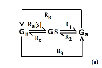
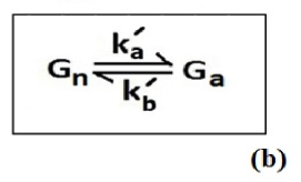
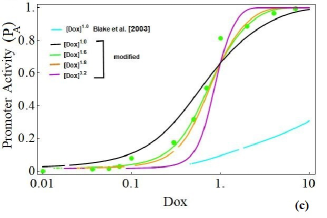
Figure 3: (a) Intermediate state assumption (b) equivalent transition (c) parameter prediction: curves for Dox power = 1.0 (cyan, Blake et al. form[3]), 1.0 (black, modified), 1.6 (green, modified), 1.8 (orange, modified) and 3.2 (violet, modified)

The kinetic equations for the reaction scheme 3a are (the terms within the parenthesis denote molecular concentration):

$$\frac{d[G_{a}]}{dt}=R_{1}[GS]+R_{B}[G_{n}]-(R_{2}+R_{R})[G_{a}]$$ (9)

$$\frac{d[GS]}{dt}=R_{a}[s^{m}][G_{n}]-R_{d}[GS]+R_{2}[G_{a}]-R_{1}[GS]$$ (10)

$$\frac{d[G_{n}]}{dt}=R_{d}[GS]+R_{R}[G_{a}]-(R_{a}[s^{m}]+R_{B})[G_{n}]$$ (11)

$$[G_{n}]+[GS]+[G_{a}]=1$$ (12)

Applying steady state condition, $\frac{d[G_{a}]}{dt}=0,\frac{d[GS]}{dt}=0,\frac{d[G_{n}]}{dt}=0$ and solving we get,

$$[G_{a}]=\frac{k_{a}^{{}^{\prime}}}{k_{a}^{{}^{\prime}}+k_{d}^{{}^{\prime}}}$$ (13)

where,

$$k_{a}^{{}^{\prime}}=R_{1}[R_{a}[s^{m}]+\frac{R_{B}}{R_{1}}R_{d}+R_{B}]$$ (14)

$$k_{b}^{{}^{\prime}}=R_{2}^{c}[R_{a}[s^{m}]+R_{d}+R_{c}]$$ (15)

with $R_{2}^{c}=(R_{2}+R_{R})$ and $R_{c}=\frac{R_{1}R_{R}+R_{2}R_{B}}{R_{2}^{c}}$.

We also assume that $R_{R}$ completely unwinds the dox from the gene and hence is a function of $[S]$ such as $R_{R}=\frac{\alpha}{[S^{m}]}$, $\alpha$ being a proportionality constant.

When the intermediate state $GS$ is absent, we have the same form of $G_{a}$ as shown in equ.13. Now from the equ.14 and 15 we can see the exact form of the GAL/dox dependent rate constants $k_{a}$ and $k_{d}$. In [3], Blake et al. used the GAL-dependent parameters as $k_{a}=0.2*GAL+0.02$ and $k_{d}=0.1*GAL+0.01+0.07/GAL+0.007/GAL$. We have tried these values and found a curve no-where near the experimental data, even-though it follows the similar sigmoid nature at much higher GAL concentrations (fig.3c). Therefore we modified the parameter values a bit and put a power $(m\geq 1)$ on dox (or GAL) to make them more general. We keep the power of dox as 1.6 for the activator-only model and 1.8 for the repressor-only model. Then, we show that the power goes near to 3.2 when both activator and repressor mutually acts competitively in the system. Using trial and error method with different numerical values we are able to achieve to fit the experimental data with theoretical curves quite nicely. We have checked by minimization of relative error and mean squared error to support the robustness of our parameter estimations. The set of parameter for activator only model are:
$k_{a}=1.2*S^{1.6}+0.2$;$\thinspace k_{d}=0.01*S^{1.6}+0.001+0.0279/S^{1.6}$ ;$\thinspace J_{m}=25-250;$$\thinspace J_{0}=0.0001;k_{m}=1$ and $Z_{th}=0.987.$

2 Two-state model where repressor acts solely

Now we focus on a two-state repressor only model (fig.4a) where mRNA is produced spontenously from normal state of gene $G_{n}$ with a leaky basal rate (very low) $J_{0}$ but no mRNA is being produced when the gene is repressed by some TFs then the gene is assumed to be OFF $(G_{r}).$ Whenever a repressor molecule get attached to the promoter it effectively inhibits the transcription. Rossi et al. [37] found repression at a particular dox concentration (i.e. $S^{1.8})$ which agrees with our theoretical plot with parameters: $k_{1}=0.02+1.8*S^{1.8}$; $k_{2}=0.001+0.14*S^{1.8}+0.097/S^{1.8}$ ; $J_{0}=0.0001;\thinspace k_{m}=1$ and $Z_{th}=0.70.$ We calculate the promoter activity given by

$P(z>Z_{th})=1-\frac{\intop_{0}^{Z_{th}}P(z)\ dz}{\intop_{0}^{1}P(z)\ dz}=1-\frac{Z_{\text{th}}^{\frac{k_{1}}{k_{m}}}\,{}_{2}F_{1}\left(\frac{k_{1}}{k_{m}},1-\frac{k_{2}}{k_{m}};\frac{k_{1}}{k_{m}}+1;\frac{k_{1}Z_{\text{th}}}{k_{1}+k_{2}}\right)}{\,{}_{2}F_{1}\left(\frac{k_{1}}{k_{m}},1-\frac{k_{2}}{k_{m}};\frac{k_{1}}{k_{m}}+1;\frac{k_{1}}{k_{1}+k_{2}}\right)}=P_{R}\thinspace(say)$.

Parameters are estimated in similar way as mentioned in previous section assuming gene-dox complex formation.

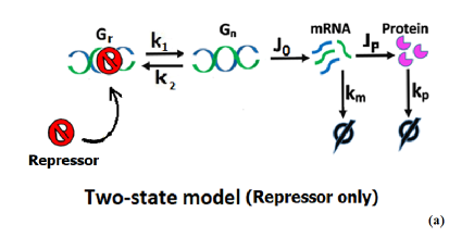
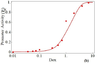
Figure 4: (a) Two-state model where repressor acts solely and inhibit the transcription (b) Dose-response curve (solid curve) fitted with experimental data (solid circles) when only repressor is present (activator absent) in promoter of gene.

3 Competitive regulatory architecture

Rossi et al. [37] have experimentally studied an eukaryotic transcriptional regulatory network where the activators and repressors bind the same sites of the promoter mutually exclusively. The important features of their work is that the activator and repressor concentrations are controlled by the single inducer doxycycline (dox). By varying the dox, they varied the activator and repressor concentration simultaneously. They observed all-or-none response when a combination of activators and repressors act on the same promoter whereas either alone show a graded response. The all-or-none and graded response of an activator-repressor system is explained by considering three states of a gene i.e., inactive ($G_{r}$), normal ($G_{n}$) and active ($G_{a}$) where the activator and repressor competes with each other to bind to the normal state, which is a open state (fig.5a) [16]. A successful binding of activator (repressor) turns the normal state into the active (inactive or repressed) state. Random transitions takes place due to random binding and unbinding events of activators and repressors. We also consider the reinitiation of transcription by RNAP II along with the competitive binding events of activators and repressors. The detail reaction scheme is shown in fig.5b.

The promoter activity calculated for the activator-repressor competitive system is

$$\begin{array}[]{cccc}P(z&>Z_{th})&=&1-\frac{\intop_{0}^{Z_{th}}P(z)\ dz}{\intop_{0}^{1}P(z)\ dz}\\ &&=&1-\frac{Z_{\text{th}}^{\frac{k_{\text{ON}}}{k_{m}}}{}_{2}F_{1}\left(1-\frac{k_{\text{OFF}}}{k_{m}},\frac{k_{\text{ON}}}{k_{m}};\frac{k_{\text{ON}}}{k_{m}}+1;\frac{k_{\text{ON}}Z_{\text{th}}}{k_{\text{OFF}}+k_{\text{ON}}}\right)}{{}_{2}F_{1}\left(1-\frac{k_{\text{OFF}}}{k_{m}},\frac{k_{\text{ON}}}{k_{m}};\frac{k_{ON}}{k_{m}}+1;\frac{k_{\text{ON}}}{k_{\text{OFF}}+k_{\text{ON}}}\right)}=P_{AR}\,(say)\end{array}$$ (16)

here, ${}_{2}F_{1}$ is a hypergeometric function.

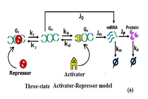
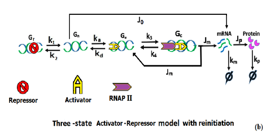
Figure 5: competitive binding of activator and repressor model (a) without reinitiation (b) with reinitiation

3.1 Parameter estimation for Activator-Repressor system

We were engaged in an attempt to find a possible set of parameters that fits the experimental data of Rossi et al. [37]. They have mentioned in their paper that the dose-response curve obtained from their experiment might follow the Hill function with different Hill coefficients. For different Hill coefficient the model behaves as repressor-only model or activator-only model and a competitive model where both activator and repressor are in competition for binding to the same region of the promoter of gene. We find that the parameter-set is much similar to those mentioned by Blake et al. [3] rather than the Hill function. Although in [3] they used GAL as activator with power 1.0 but here we keep the powers of dox (or GAL) as 1.8 for repressor and 1.6 for activator-only following the Hill coefficient values obtained in [37] (fig. 6a and fig. 6b). In order to explore the competitive model we consider a simplified equivalent two-state model (fig. 6d) of reaction scheme 5a. Here, we neglect $J_{0}$ in comparison with $J_{m}\ or\ J_{1}$ (as $J_{0}<<J_{1}).$ Moreover, it is admitted by Karmakar [16] that, this assumption does not make any qualitative change in PDF and we have checked, it also holds true in case of mean mRNA and noise strength. Karmakar in [16] also mentioned that, the deterministical determination of probability for a three state activator-repressor competitive binding model is very difficult when basal rate $J_{0}$ is involved. The deterministic reaction rate equations for reaction scheme shown in fig.5a are given as:

$$\frac{d[G_{r}]}{dt}=k_{2}[G_{n}]-k_{1}[G_{r}]$$ (17)

$$\frac{d[G_{n}]}{dt}=k_{d}[G_{a}]-k_{a}[G_{n}]$$ (18)

$$\frac{d[G_{a}]}{dt}=k_{a}[G_{n}]-k_{d}[G_{a}]$$ (19)

$$\frac{d[M]}{dt}=J_{1}[G_{a}]+J_{0}[G_{n}]-k_{m}[M]$$ (20)

$$[G_{n}]+[G_{r}]+[G_{a}]=1$$ (21)

In steady state, $\frac{d[M]}{dt}=0$ and we have

$$[M]=\frac{J_{1}[G_{a}]+J_{0}[G_{n}]}{k_{m}}\simeq\frac{J_{1}}{k_{m}}[G_{a}]$$ (22)

We may neglect the small contribution of $J_{0}$ with respect to $J_{1}.$

Applying the steady state condition, $\frac{d[G_{a}]}{dt}=0,\frac{d[G_{r}]}{dt}=0,\frac{d[G_{n}]}{dt}=0$ and solving we get

$$[G_{a}]=\frac{k_{1}k_{a}}{k_{1}k_{a}+k_{d}(k_{1}+k_{2})}$$ (23)

Therefore,

$$[M]=\frac{J_{1}}{k_{m}}\frac{k_{1}k_{a}}{k_{1}k_{a}+k_{d}(k_{1}+k_{2})}$$ (24)

Now, the reaction rate equations for the simplified equivalent model (see reaction scheme 6d) are:

$$\frac{d[G_{r}]}{dt}=k_{OFF}[G_{a}]-k_{ON}[G_{r}]$$ (25)

$$\frac{d[M]}{dt}=J_{m}[G_{a}]-k_{m}[M]$$ (26)

$$[G_{r}]+[G_{a}]=1$$ (27)

steady state condition gives

$$[M]=\frac{J_{m}}{k_{m}}\frac{k_{ON}}{(k_{ON}+k_{OFF})}$$ (28)

writing $J_{m}=J_{1}$ and comparing equ.24 with equ.28 we get,

$$k_{ON}=k_{1}k_{a}$$ (29)

$$k_{OFF}=k_{d}(k_{1}+k_{2})$$ (30)

Now, we get a form of the main parameters that have a dominant role over the others for the system. We see that multiplication of the component-parameters like $k_{1},k_{a},k_{d},k_{2},etc.$ to form $k_{ON}$ and $k_{OFF}$ actually leads to a addition of powers of dox molecule. Theoretically, we obtain the power of dox (S) for activator-repressor competitive system as 3.4 which has a close agreement with the experimentally observed value 3.2 (fig.6c). Here, by taking the dox-dependent parts of the component-parameters and using equ.29 and equ.30 we get,

$k_{ON}=1.08*S^{3.4}$ and $k_{OFF}=0.0032*S^{3.4}+0.0027/S^{3.4}+0.0089*S^{0.2}+0.00097/S^{0.2}$. On top of that, while working with the parameter estimation we notice that beside the power of dox there are other parameters like $Z_{th}$ that effect the slope of the curves. We can put $Z_{th}$ at any value between 70% to 99% to find a best fit curve. Moreover, to show the robustness of our parameter estimation we examine the sensitivity against the parameters and minimize the standard errors for each data points by using chi-square fitting method (see Appendix-B).

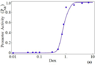
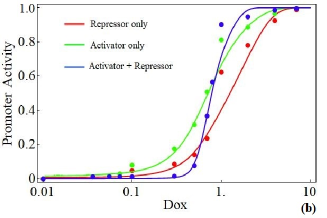
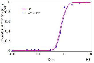
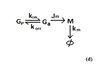
Figure 6: (a) Dose-response curve (solid curve) fitted with experimental data (solid circles) when both activator and repressor competes to sit on the promoter of the gene.(b) Dose-response curve (solid curves: green- activator-only, red- repressor-only and blue- activator-repressor in competition) fitted with experimental data (solid circles: green- activator-only, red- repressor-only and blue- activator-repressor in competition). (c) Dose-response curve for activator-repressor showing a close agreement of theoretically obtained curve with dox power combination of 3.4 & 0.2 (blue curve) with experimentally found value of 3.2 (pink curve). (d) Two-state equivalent simplified circuit of the three-state activator-repressor competitive model.

3.2 Stochastic Analysis

Let, there are $l$ copy number of a particular gene exist in the cell. We consider the reaction scheme in fig.5b and let $P(n_{1},n_{2},n_{3},n_{4},n_{5},t)$be the probability that at time t, there are $n_{4}$ number of mRNAs and $n_{5}$ number of proteins molecules with $n_{3}$ number of genes in the initiation complex ($G_{c}$), $n_{2}$ number of genes in the active state ($G_{a}$) and $n_{1}$ number of genes in the normal state ($G_{n}$). The number of gene in the inactive states ($G_{r}$) are ($l-n_{1}-n_{2}-n_{3}$). The time evolution of the probability (assuming $J_{0}=0)$ is given by

$$\begin{array}[]{ccc}\frac{\partial P(n_{i},t)}{\partial t}&=&k_{1}[\{l-(n_{1}-1+n_{2}+n_{3})\}P(n_{1}-1,n_{2},n_{3},n_{4},n_{5},t)\\ &&-\{l-(n_{1}+n_{2}+n_{3})\}P(n_{i},t)]\\ &&+k_{2}[(n_{1}+1)P(n_{1}+1,n_{2},n_{3},n_{4},n_{5},t)-n_{1}P(n_{i},t)]\\ &&+k_{a}[(n_{1}+1)P(n_{1}+1,n_{2}-1,n_{3},n_{4},n_{5},t)-n_{1}P(n_{i},t)]\\ &&+k_{d}[(n_{2}+1)P(n_{1}-1,n_{2}+1,n_{3},n_{4},n_{5},t)-n_{2}P(n_{i},t)]\\ &&+k_{3}[(n_{2}+1)P(n_{1},n_{2}+1,n_{3}-1,n_{4},n_{5},t)-n_{2}P(n_{i},t)]\\ &&+k_{4}[(n_{3}+1)P(n_{1},n_{2}-1,n_{3}+1,n_{4},n_{5},t)-n_{3}P(n_{i},t)]\\ &&+J_{m}[(n_{3}+1)P(n_{1},n_{2}-1,n_{3}+1,n_{4}-1,n_{5},t)-n_{3}P(n_{i},t)]\\ &&+k_{m}[(n_{4}+1)P(n_{1},n_{2},n_{3}n_{4}+1,n_{5},t)-n_{4}P(n_{i},t)]\\ &&+J_{p}[n_{4}P(n_{1},n_{2},n_{3},n_{4},n_{5}-1,t)-n_{4}P(n_{i},t)]\\ &&+k_{p}[(n_{5}+1)P(n_{1},n_{2},n_{3},n_{4},n_{5}+1,t)-n_{5}P(n_{i},t)]\end{array}$$ (31)

where, i = 1,2,……, 5

We can derive the mean, variance and the Fano factor of mRNAs and proteins from the moments of equation (31) with the help of a generating function

(Appendix-A). The mean mRNA and protein are given by

$$m^{CWR}=\frac{J_{m}k_{1}k_{a}k_{3}}{l_{3}k_{m}};\quad\quad p^{CWR}=\frac{m^{CWR}\,J_{p}}{k_{p}}$$ (32)

The expression for the Fano factors at mRNA and protein level are given by

$$\begin{array}[]{ccccc}FF_{m}^{CWR}&=&1-&m^{CWR}-&\frac{J_{m}k_{3}(h_{2}k_{m}+k_{1}k_{a})}{(k_{3}(h_{2}(J_{m}+k_{4})-k_{1}k_{a})+h_{8}(k_{a}(k_{d}-k_{1})-h_{2}h_{6}))k_{m}}\end{array}$$ (33)

$$\begin{array}[]{ccccccc}FF_{p}^{CWR}&=&1-&p^{CWR}&+\frac{J_{p}J_{m}k_{3}(k_{m}k_{p}-k_{1}k_{a})}{l_{10}}&+\frac{J_{p}J_{m}k_{3}(h_{2}k_{m}+k_{1}k_{a})}{l_{12}}&+\frac{J_{p}}{k_{m}+k_{p}}\end{array}$$ (34)

where $l_{12}=l_{1}l_{10}(k_{1}k_{a}(k_{3}+l_{8})-k_{3}l_{2}J_{m}-k_{3}k_{4}l_{2}-k_{a}k_{d}l_{8}+l_{6}l_{8}l_{2});$

$l_{11}=l_{10}+l_{1}(k_{3}J_{m}-k_{1}k_{a}+k_{a}k_{d}+k_{3}k_{4}-l_{4}l_{5}-l_{4}l_{8}-l_{6}l_{8};$

$l_{10}=(k_{3}l_{9}+l_{7}(k_{a}k_{d}-k_{a}k_{1}-l_{4}l_{5}))k_{p}(k_{m}+k_{p});$

$l_{9}=(l_{4}(J_{m}+k_{4})-k_{1}k_{a});\quad$ $l_{8}=J_{m}+k_{4}+k_{m};$  $l_{7}=J_{m}+k_{4}+k_{p};$

$l_{6}=k_{d}+k_{3}+k_{m};$  $l_{5}=k_{d}+k_{3}+k_{p};$  $l_{4}=k_{1}+k_{2}+k_{a}+k_{p};$

$l_{3}=k_{1}k_{a}k_{3}+(k_{1}k_{d}+k_{2}k_{d}+k_{1}k_{a})(J_{m}+k_{4})$;

$l_{2}=k_{1}+k_{2}+k_{a}+k_{m}$;  $l_{1}=(k_{m}+k_{p})k_{m}k_{p};$

For the without-reinitiation scheme (fig.5a), the required expression for the mean level of mRNA ($m^{CWTR}$) and protein ($p^{CWTR}$) are given by

$$m^{CWTR}=\frac{J_{m}k_{1}k_{a}}{r_{1}k_{m}};\quad\quad p^{CWTR}=\frac{m^{CWTR}\,J_{p}}{k_{p}}$$ (35)

The corresponding Fano factors at mRNA ($FF_{m}^{CWTR}$) and protein ($FF_{p}^{CWTR}$) level are given by

$$FF_{m}^{CWTR}=1-m^{CWTR}+\frac{J_{m}(r_{5}k_{m}+k_{1}k_{a})}{r_{2}k_{m}}$$ (36)

$$FF_{p}^{CWTR}=1-p^{CWTR}+X$$ (37)

where, $X=\frac{J_{p}}{k_{m}+k_{p}}+\frac{J_{p}J_{m}k_{1}k_{a}}{r_{9}k_{p}(k_{m}+k_{p})}+\frac{J_{p}J_{m}(r_{6}k_{m}+r_{9})}{r_{9}(k_{m}+k_{d})(k_{m}+k_{p})}+\frac{J_{p}J_{m}k_{a}k_{d}(k_{m}+k_{1})r_{10}}{r_{4}(k_{m}+k_{d})(k_{m}+k_{p})k_{m}};$

$r_{10}=r_{1}+r_{3}k_{m}+r_{7}k_{p};$  $r_{9}=r_{6}(k_{p}+k_{d})+k_{a}(k_{1}-k_{d});$ $r_{8}=r_{6}+k_{d};$

$r_{7}=r_{8}+k_{m};$ $r_{7}=r_{8}+k_{m};$ $r_{6}=k_{1}+k_{2}+k_{a}+k_{p};$ $r_{5}=k_{1}+k_{2}+k_{a}+k_{m};$

$r_{4}=r_{2}(r_{8}k_{p}+r_{1});$ $r_{3}=r_{5}+k_{d};$ $r_{2}=r_{1}+r_{3}k_{m};$ $r_{1}=k_{1}k_{a}+k_{1}k_{d}+k_{2}k_{d}.$

Here, ${}^{\prime}C^{\prime}$ in the superscripts stands to indicate competitive binding, ${}^{\prime}WTR^{\prime}$ represents without-reinitiation and ${}^{\prime}WR^{\prime}$ implies with-reinitiation model.

The experimental values of the rate constants $k_{i}$ (i = 1,2,…,6) are not available for the competitive activator-repressor model (fig.5a). In the previous sections, we have tried to find out a probable set of parameter that fits the experimental points. In this way, the activator and repressor concentrations are controlled by the single inducer doxycycline (dox, denoted by S). We notice that the theoretically obtained parameter-set is quite similar to the parameters used by Blake et al. in a synthetic GAL1* promoter in yeast [3], except they have used GAL as activator and aTc-bounded tetR as repressor. We want to check the behavior of competitive system under the parameter set used in [3] and compare the results with the non-competitive one [42]. The reaction rate constants chosen from [3] for the competitive system are: $k_{a}=0.02+0.2*GAL,$$k_{d}=0.01+0.1*GAL+0.077/GAL$, $k_{3}=50,k_{4}=10,k_{1}=10,\,k_{2}=200*(tetR)^{2}/[1+(C_{i}*aTc)^{4}]^{2},\thinspace$$J_{m}=1,k_{m}=1,J_{p}=5,k_{p}=0.0125,tetR=100,C_{i}=0.1$.

In the next step, we study the behavior of mean protein levels and noise strength with respect to the inducer (GAL and aTc) and transcriptional efficiency respectively. We note that, the mean protein level varies with GAL and aTc in similar fashion in presence and/or absence of reinitiation (fig.5a) as in the non-competitive regulatory archietecture [42]. The variation of noise strength with transcriptional efficiency for fixed aTc (500 ng/ml) is again similar with the non-competitive regulatory archietecture [42]. Interestingly, the variation of noise strength with transcriptional efficiency for fixed GAL (2%) is different from that obtained from the non-competitive regulatory architecture [42]. We notice that, the noise strength is maximum at the very beginning of the transcriptional efficiency rather than the intermediate level, as shown in fig. 2c and 2e of [42].

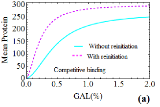
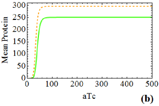
Figure 7: Variation of mean protein: (a) with GAL when aTc is fixed (b) with aTc when GAL is fixed. Solid (dashed) lines are drawn from analytical calculation corresponding to the reaction scheme 5a and 5b respectively. All rate constants are chosen from [3].

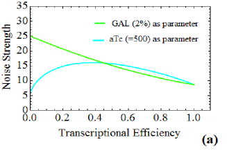
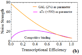
Figure 8: Variation of the noise strength with transcriptional efficiency: (a) green (cyan) line is drawn analytically with 2% GAL concentration (with aTc = 500 ng/ml) from the reaction scheme 5a (b) orange (violet) solid line is drawn analytically with 2% GAL concentration (with aTc = 500 ng/ml) from the reaction scheme 5b, following the same parameter values as used by Blake et al. in [3].

4 Comparison between competitive and non-competitive architecture

In this section, we study the nature of mean products (mRNA/Protein) and their corresponding noise strengths (the Fano factors) for both competitive and non-competitive binding circuits. We also observe the relative changes of these two physical quantities when the reinitiation is taken under consideration (presented by the dashed lines in characteristic curves) for both the architectures. Although the non-competitive circuit and its behaviour was rigorously studied by Das AK in [42], we put the model diagram here to understand the comparison in much better way. In a competitive network, activator and repressor compete for a common binding region of promoter. As a result, the gene is in either active (ON) or repressed (OFF) state, except a normal state $(G_{n})$. Whereas, there could be four possible genetic states: normal $(G_{n})$, active $(G_{a})$, active-repressed $(G_{ar})$ and repressed $(G_{r})$ as shown in fig. 9a.

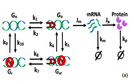
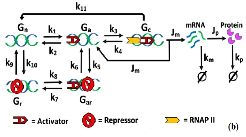
Figure 9: Non-competitive binding of activator and repressor (a) without reinitiation (b) with reinitiation and with a reverse transition via $k_{11}$

A reverse transition is incorporated via $k_{11}$ from the initiation complex $(G_{c},$ arise due to reinitiation) to the normal state $(G_{n})$ as there is a possibility of simultaneous unwinding of RNAP-II and activator molecule, that can not be neglected [42]. We find that this reaction path finely affects the mean expression and noise strength of the non-competitive circuit [42] and the competitive one as well. We subsequently study the behavioral changes of competitive binding model from the non-competitive model under the same reaction rate constants in the next sections.

4.1 Role of reinitiation under the action of aTc and GAL: anomalous behavior at lower aTc concentration

In this section, we focus on some characteristic differences mainly, that appear due to reinitiation when GAL (activator) and aTc (repressor) is operating competitively or non-competitively.

Although, no observable difference is found in the variation of mean mRNA (mean protein) against GAL with different aTc values between both the circuits (fig.10a, 10b, 10e and 10f) rather, they offer the same expression levels under identical rate constants (chosen from [3] with $J_{m}=15$ and $k_{11}=0$). It is noticeable that, noise strength (the Fano factor) in the super-Poissonian regime ($FF_{m}>1)$ is higher in competitive circuit than non-competitive circuit (fig. 10c,d,g,h and fig. 11c,d,g,h).

• We further notice that, each solid curve (presenting without-reinitiation) has a point of intersection with the dashed curve (represents with-reinitiation) at a particular GAL value (where, $m^{WR}=m^{WTR}\ and\ p^{WR}=p^{WTR})$, beyond which $m^{WR}\thinspace(or,\thinspace p^{WR})<m^{WTR}\thinspace(or,\thinspace p^{WTR})$. The only exception holds for the curves with $aTc<45$ ng/ml when $m^{WR}\thinspace(or,\thinspace p^{WR})>m^{WTR}\thinspace(or,\thinspace p^{WTR})$ always.

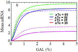
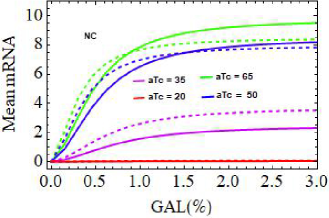
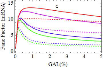
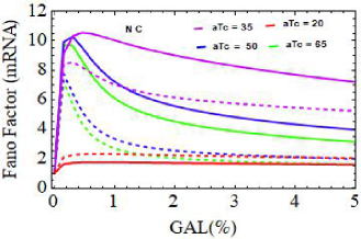
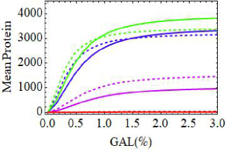
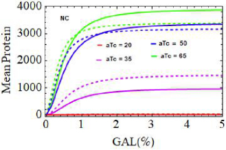
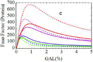
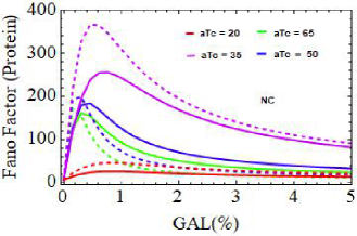
Figure 10: Variation of mean mRNA with GAL for different aTc concentration (a) in Competitive and (b) in non-competitive network.
Variation of the Fano factor (mRNA level) with GAL for different aTc concentration (c) in Competitive and (d) in non-competitive network.
Variation of mean Protein with GAL for different aTc concentration (e) in Competitive and (f) in non-competitive network.
Variation of the Fano factor (protein level) with GAL for different aTc concentration (g) in Competitive and (h) in non-competitive network.
The solid curves are corresponding to the system without reinitiation (reaction scheme 5a and 9a respectively) and dashed curves are corresponding to the reaction scheme with reinitiation (fig.5b and 9b respectively). Each plot containing solid/dashed curves with aTc=20 ng/ml (red), aTc=35 ng/ml (violet), aTc=50 ng/ml (blue) and aTc=65 ng/ml (green). The rate constants are chosen from [3] with $J_{m}=15$ and $k_{11}=0$.

• On the other hand, the curves correspond to aTc = 20 show some anomaly. Usually, $FF_{m}^{WTR}>FF_{m}^{WR}$ for all values of aTc in competitive and non-competitive circuit (fig. 10c, and 10d) as well, except for aTc = 20 in non-competitive circuit.

• Although, $FF_{m}^{WTR}>FF_{m}^{WR}$ while  $FF_{p}^{WTR}<FF_{p}^{WR}$ for aTc = 20 in the competitive model (fig. 10c and 10g).

• However, for aTc > 45, $\,FF_{p}^{WR}$ falls below $\thinspace FF_{p}^{WTR}\,$ just after attending a quick peak value at lower GAL concentrations.

• A minute observation finds out that $FF_{m}(FF_{p})$ at $50<aTc<65$ rises sharply then get a certain stability (straight horizontal part) for a very short range of GAL (0.1 - 0.3 unit) and finally falls with increasing GAL. This feature is absent in other values of aTc.

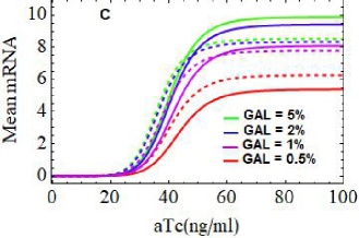
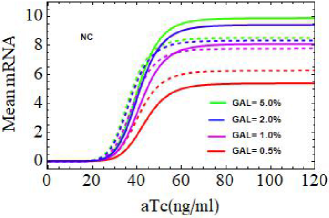
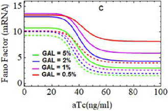
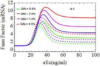
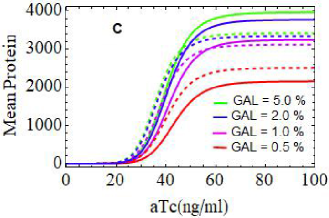
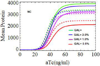
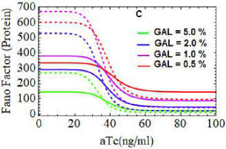
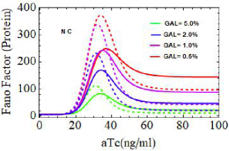
Figure 11: Variation of mean mRNA with aTc for different GAL concentration (a) in Competitive and (b) in non-competitive network.
Variation of the Fano factor (mRNA level) with aTc for different GAL concentration (c) in Competitive and (d) in non-competitive network.
Variation of mean Protein with aTc for different GAL concentration (e) in Competitive and (f) in non-competitive network.
Variation of the Fano factor (protein level) with aTc for different GAL concentration (g) in Competitive and (h) in non-competitive network.
The solid curves are corresponding to the system without reinitiation (reaction scheme 5a and 9a respectively) and dashed curves are corresponding to the reaction scheme with reinitiation (fig.5b and 9b respectively). Each plot containing solid/dashed curves with GAL=0.5% (red), GAL=1.0% (violet), GAL=2.0% (blue) and GAL=5.0% (green). The rate constants are chosen from [3] with $J_{m}=15$ and $k_{11}=0$.

The sigmoid nature of the mean expressions with aTc implies that there exists three regions of operation: cut-off, active or sensitive and saturation [42]. A high value of aTc implies low repression while lower aTc concentration make the system to OFF state due to high repression. The parameters $k_{2}$ in competitive model and $k_{10}$ in non-competitive system contain aTc bounded tetR act as repressor binding rates. We have found some interesting features of mean expressions and the Fano factors for both models (fig. 11a to 11h).

• We notice that, $m^{WR}\thinspace(or,\thinspace p^{WR})>m^{WTR}\thinspace(or,\thinspace p^{WTR})$ at the region of sensitivity ($20\leq aTc\leq 60$) but $m\thinspace(or,\thinspace p^{WR})<m^{WTR}\thinspace(or,\thinspace p^{WTR})$ at saturation region (aTc > 60), only exception holds for curves with lower GAL concentrations ($\sim\thinspace$0.5%).

• It is clearly observed from fig. 10c that, $FF_{m}^{WTR}>FF_{m}^{WR}$ in all three regions while this behavior is observed beyond a point of intersection at a certain aTc value for each pair of curves in the non-competitive model (fig. 10d). We further notice in fig. 10c that, the noise (WTR) for GAL = 0.5% is slightly lesser than the noise for GAL = 1.0% at the early stages of aTc concentration ($\sim$aTc $<$ 35), after that it goes higher of GAL =1.0% curve for higher aTc values. No such anomaly has been found in non-competitive system.

• Interestingly, there is a major difference found in noise profile in protein level, which arises due to the reinitiation effect that, $FF_{p}^{WR}>>FF_{p}^{WTR}\,$ at initial values of aTc and at a particular value of aTc each WR curve crosses over the WTR curve. After that WR curves goes lower the WTR curves at higher aTc concentrations. Again, a noticeable anomaly is found for fig. 11g that, curve corresponds to GAL = 0.5% goes slightly lower to the curve for GAL = 1.0% till aTc $\simeq$ 31.0 (WTR) and aTc $\simeq$ 36.0 (WR) instead of going higher. However, no such anomaly is found in case of non-competitive circuit.

4.2 Noise reducing factors

We notice that noise can be enhanced or reduced by reinitiatian from fig. 10 and fig. 11. It is also seen that competitive binding model shows much noise than the non-competitive one. Now, we check whether noise can be reduced much below to the Poissonian level ($FF_{m}=1)$. Fig. 12 reveals that it is possible if the value of $k_{4}$ is reduced from 10 to 1. According to Blake et al. [3] when $k_{4}=1$ the RNAP-II binds much tightly with the promoter even when repressor is rarely present which results in much reduction of noise for the circuits of both types. Moreover, we find that noice in the competitive model can be reduced much further than non-competitive one in the sub-Poissonian region ($FF_{m}<1)$, corresponding to $k_{4}=10$ (fig. 12a and 12b) or $k_{4}=1$ (fig. 12c and 12d).

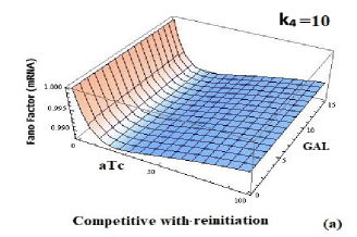
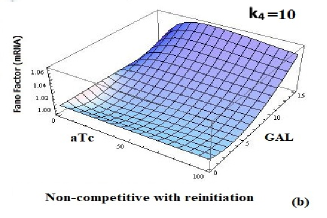
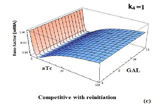
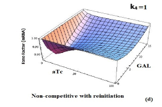
Figure 12: Role of $k_{4}$ in reducing noise strength: variation of the Fano factor at mRNA level with $k_{3}$ and $J_{m}$ (a) competitive circuit with $k_{4}=10$, (b) non-competitive circuit with $k_{4}=10$, (c) competitive circuit with $k_{4}=1$ and (d) non-competitive circuit with $k_{4}=1.$ Other parameter values are same as in [3] with GAL = 30%, aTc = 65 ng/ml, $J_{m}=15$ and $k_{11}=0.$

Conclusions

The regulation of gene expression through transcription factors (TFs) and control of noise are biologically significant [44, 45, 46] to respond to the intra-cellular and external environmental changes as well [25]. They are also important in various medical applications [46-48]. For example, the TFs (activators and repressors) can act as a tumor suppressor in prostate cancer [44]. The noise, arising due to various stochastic events in gene expression are used to modulate reactivation of HIV from latency (a quiescent state, that is a major barrier to an HIV cure). Noise suppressors stabilized latency while noise enhancers reactivates latent cells [47] . On the contrary, the noisy expression can be beneficial to a population of genetically identical cells by composing phenotypic heterogeneity [6, 10, 23, 24, 25].

In this paper, we have studied a gene transcription regulatory architecture where activator and repressor molecules bind the promoter of gene in a competitive fashion. There may be various mode of competition among the TFs and promoter binding sites [16, 39]. Some theoretical studies have explored the kinetics and recorded the effects of TFs on noise [39, 40, 41]. Meanwhile, we found an experimental study on a competitive binding network performed by Rossi et al. [37]. Almost a decade later, Yang and Ko [38] tried to explain the experimental result with the help of stochastic simulation. However, both the approaches were unable to explain the collective (Hill coefficient) and stochastic behavior of the three-state competitive activator-repressor system due to the lack of detailed kinetics and parameter values. We further found that, Karmakar [16] also found the similar distributions (PDF) as in [37] by theoretical analyses and explained how the response changes from graded to binary in presence of either activator or repressor or both. However, the required parameter values or the exact relation of parameters with dox was still remain unavailable. Moreover, the above mentioned works did not focus on the noise profile of the three-state competitive activator-repressor system. In recent work, Braichencho et al. [32] modeled a three-state activator-repressor system where they have studied a proximal promoter-pausing which can be effectively described by a two-state model in some limiting case. Another competitive model was proposed in [48] where the regulation of gene expression can occur via two cross talking parallel pathways. Although, our approaches and investigations are different in the present work.

The goal of our study is to fabricate a framework to explain the model with a proper theory supported by analytical and/or simulation methods. Consequently, we developed a theory that offers detailed chemical kinetics of the competitive activator-repressor system and a most probable set of parameter values that fit the experimental data [37] quite nicely. The dox-dependent parameters, here we found, having very much similar form that proposed by Blake et al. in [3] instead of the Hill type [37, 38]. However, in [3] the authors did not clearly mention how the structure of these parameters are formed. Hence, we have designed an analytical treatment by assuming intermediate gene-dox complex formation to determine the exact forms of parameters (i.e. relation with dox) and revealed how the mean expression and noise varies with the changes of these parameter values. The robustness of our parameter estimation is supported by the minimization of relative error and the mean squared error given in the appendix-B. We admit that the choice of rate constants is not unique, there can be other sets of parameters that may give better fitting of analytical curves with the experimental results. We have found the important parameters that govern the stochastic noise of the circuit. We have also noticed some anomalous behaviour of both mean and the Fano factor with the variation of activator (GAL) and/or repressor (aTc) whenever reinitiation of transcription was taken under consideration. On top of that, we have made a comparison of characteristics between competitive and non-competitive architecture and noticed that just as the noise in competitive circuit is high in the super-Poissonian region, its noise can be reduced much further in the sub-Poissonian regime in comparison with the the non-competitive circuit. However, the mean expression levels remain same under identical set of rate constants. The reason behind such behaviour is subject to further analysis which we have not performed here.

Our proposed theory may applicable in synthetic biology to understand the the architecture of interactions which may buffer the stochasticity inherent to gene transcription of a complex biological system. By using our analytical approach, it is possible to predict the mean and standard deviation of the number of transcribed mRNAs/proteins. There can be further extensive study on the model considering the effect of other parameters that are not considered in present analysis. The availability of a well-designed analytical theory with detailed reaction kinetics of that model could be the powerful tools for future research and analysis for the similar or comparable genetic networks.

Glossary

• Transcription factor : Transcription factors (TFs) are proteins which have DNA binding domains with the ability to bind to the specific sequences of DNA (called promoter). They controls the rate of transcription. If they enhance transcription they are called activators and termed as repressors if inhibit transcription.

• Fano factor and Noise strength : The Fano factor is the measure of deviations of noise from the Poissonian behavior and is defined as [42, 43] ,

$$Fano\thinspace factor=\frac{variance}{mean}=\frac{(standard\thinspace deviation)^{2}}{mean}$$

So, for a given mean, smaller the Fano factor implies smaller variance and thus less noise. Therefore, the Fano factor gives a measure of noise strength which is defined (mathematically) as [2],

$$noise\thinspace strength=\frac{variance}{mean}=\frac{(standard\thinspace deviation)^{2}}{mean}$$

So, the Fano factor and noise strength are synonymous.

• Transcriptional efficiency : Transcriptional efficiency is the ratio of instantaneous transcription to the maximum transcription [3].

Appendix A

In an attempt to find out the expressions of mean mRNA (protein) and the corresponding Fano factors, we have used a moment generating function which is defined as,

$$F(z_{i},t)=\sum_{n=0}^{\infty}z_{i}^{n_{i}}p(n_{i},t)$$ (38)

Here, $i=1,2,......,5$.

we have,

$$\begin{array}[]{ccc}\frac{\partial F(z_{i},t)}{\partial t}&=&\sum_{n=0}^{\infty}z_{i}^{n_{i}}\frac{\partial p(n_{i},t)}{\partial t}\\ &=&k_{1}(z_{1}-1)[lF-z_{1}\frac{\partial F}{\partial z_{1}}-z_{2}\frac{\partial F}{\partial z_{2}}-z_{3}\frac{\partial F}{\partial z_{3}}]\\ &&+k_{2}(1-z_{1})\frac{\partial F}{\partial z_{1}}+k_{a}(z_{2}-z_{1})\frac{\partial F}{\partial z_{1}}+k_{d}(z_{1}-z_{2})\frac{\partial F}{\partial z_{2}}\\ &&+k_{3}(z_{3}-z_{2})\frac{\partial F}{\partial z_{2}}+k_{4}(z_{2}-z_{3})\frac{\partial F}{\partial z_{3}}\\ &&+J_{m}(z_{2}z_{4}-z_{3})\frac{\partial F}{\partial z_{3}}+k_{m}(1-z_{4})\frac{\partial F}{\partial z_{4}}\\ &&+J_{p}(z_{5}-1)z_{4}\frac{\partial F}{\partial z_{4}}+k_{p}(1-z_{5})\frac{\partial F}{\partial z_{5}}\end{array}$$ (39)

In steady state, $\frac{\partial F(z_{i},t)}{\partial t}=0$ and for total probability, $F((z_{i}=1,0)=1$

Now, by setting [$\frac{\partial}{\partial z_{1}}(\frac{\partial F}{\partial t})]_{z_{i}=1}=0$, we get $\frac{\partial F}{\partial z_{1}}=f_{1}(say)=\thinspace<n_{1}>\thinspace=$ average number of gene at state $G_{a}$.

similarly, by setting [$\frac{\partial}{\partial z_{1}}(\frac{\partial^{2}F}{\partial z_{1}\partial t})]_{z_{i}=1}=0$ will give $\frac{\partial^{2}F}{\partial z_{1}^{2}}=f_{11}(say)$ and so on. Proceeding in the same way we obtain ,

$$f_{4}=\thinspace<n_{4}>\thinspace=mean\thinspace mRNA$$

and

$$f_{5}=\thinspace<n_{5}>\thinspace=mean\thinspace Protein$$

$$Fano\thinspace factor\thinspace(mRNA)=\frac{variance\thinspace of\thinspace mRNA}{mean\thinspace mRNA}=\frac{f_{44}+f_{4}-f_{4}^{2}}{f_{4}}$$

$$Fano\thinspace factor\thinspace(Protein)=\frac{variance\thinspace of\thinspace Protein}{mean\thinspace Protein}=\,\frac{f_{55}+f_{5}-f_{5}^{2}}{f_{5}}$$

In addition, if the contributions of basal rate $J_{0}$ and the reverse transition $k_{R}$ (or $k_{11})$ are taken under consideration, there would be two more terms in equ. 39as,

$\,J_{0}(z_{4}-z_{1})\frac{\partial F}{\partial z_{1}}$ and $k_{R}(z_{1}-z_{3})\frac{\partial F}{\partial z_{3}}$.

Appendix B

• Model fitting parameters: We proposed an analytical theory that fits very much to the experimental result, performed by Rossi et al. [37]. The dox dependent parameters, here we found, having very much similar form that proposed by Blake et al. in [3] instead of Hill type [37, 38]. However, in [3] the authors did not clearly mention how the structure of these parameters are formed. Hence, we design an analytical treatment as described in the main text to determine the forms of the parameters $k_{a}$, $k_{1}$, $k_{2}$ and $k_{d}$. While for the best estimates of other parameters are revised through trial and error to minimize the sum of squared error (SSE) and the mean square error (MSE). We also provide the parameter sensitivity plot in fig. 13a. Moreover, we calculate and check the relative percentile error (RE) for each curves by using the formula,

  $$RE=\frac{y_{T}-y_{E}}{y_{E}}.100\%$$ (40)

where, T stands for theoretical and E stands for experimental.

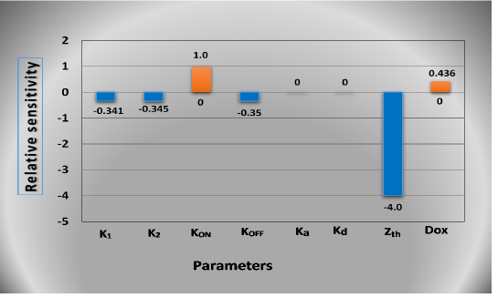
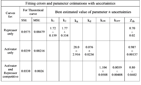
Figure 13: (a) sensitivity of parameters (b) minimized error of fitting and parameter estimation with uncertainties

• Uncertainty in fitted parameters : The uncertainty of the parameter estimates, is generally expressed by the mean square errors, is proportional to the SSE (SSWE) and inversely proportional to the square of the coefficient of sensitivity of the model parameters [49]. The mean square fitting error is

  $$\sigma^{2}=\frac{1}{n-r}\sum_{i=1}^{n}[w_{i}(y_{T}-y_{E})]^{2}=\frac{Sum\thinspace of\thinspace squared\thinspace weighted\thinspace error}{(n-r)}$$ (41)

  n is the number of observations and r is the number if parameters being determined. The weighting factor, $w_{i}$ is determined by the slope of the curve at each data point.

The sensitivity ($\mathscr{\mathscr{\mathscr{\mathfrak{\mathcal{S}}}}}$) of a function $f(r)$ over the parameter $r$ is given by

$$\mathcal{S}=\frac{r}{f(r)}.\frac{\partial f(r)}{\partial r}$$ (42)

We obtain the sensitivity of the Fano factor (mRNA) over the fitting parameters and calculate MSE of each parameter keeping others as constant.

$$MSE=\frac{\sigma^{2}}{\sum_{i=1}^{n}[\frac{\partial f(r)}{\partial r}]^{2}}$$ (43)

where the denominator is the coefficient of sensitivity, squared and summed over all observations.

The $Z_{th}$ is the most sensitive parameter and it was kept constant for each case. We also notice that sensitivity is independent of $J_{1},$$J_{0}$, $k_{a}$ and $k_{d}$ as well. We found that, the promoter activity is sensitive within a small range of values of the chosen parameters. The best parameter estimation and minimization of errors (see fig. 13b) support the robustness of our result. The square root of the MSE is the standard deviation, and the approximate 95% confidence interval for r is [49]

$$[r]_{95\%}=\Re\pm 2\surd MSE$$ (44)

$\Re$ is the best estimate value of parameter $r.$

Appendix C

In this section we provide some 3D figures (fig. 14) for the clear visualization of the variation of the noise strength (in terms of the Fano factor) with GAL (activator) and aTc (repressor) for both competitive and non-competitive circuit. One can see the noise is higher in competitive circuit than non-competitive one although their behaviour against the inducers is different. This figures also compare the effect of reinitiation with ease.

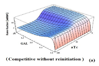
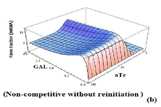
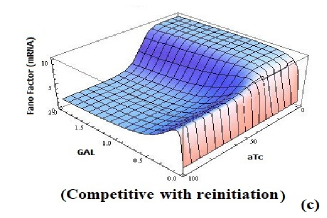
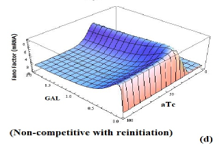
Figure 14: Variation of noise ($FF_{m})$ with GAL and aTc: (a) Competitive without reinitiation (b) Non-competitive without reinitiation (c) Competitive with reinitiation (d) Non-competitive with reinitiation. Rate constants chosen from [3] with $J_{m}=15$ and $k_{11}=0.$

References

- [1] M.B. Elowitz, A.J. Levine, E.D. Siggia, P.S. Swain, Stochastic gene expression in a single cell. Science 297, 1183 (2002)
- [2] E.M. Ozbudak, M. Thattai, I. Kurtser, A.D. Grossman, A.V. Oudenaarden, Regulation of noise in the expression of single gene. Nature Genet. 31, 69 (2002)
- [3] W.J. Blake, M. Kaern, C.R. Cantor, J.J. Collins, Noise in eukaryotic gene expression. Nature 422, 633 (2003)
- [4] J.M. Raser, E.K. O’Shea, Noise in gene expression: origins, consequences, and control. Science 309, 2010 (2005)
- [5] I. Golding, J. Paulsson, S.M. Zawilski, E.C. Cox, Realtime kinetics of gene activity in individual bacteria. Cell 123, 1025 (2005)
- [6] W.J. Blake, G. Balazsi, M.A. Kohanski, F.J. Isaas, K.F. Murphy, Y. Kuang, C.R. Cantor, D.R. Walt, J.J. Collins, Phenotypic consequences of promoter-mediated transcriptional noise. Mol. Cell 24, 853 (2006)
- [7] A. Raj, C.S. Peskin, D. Tranchina, D.Y. Vargas, S. Tyagi, Stochastic mRNA synthesis in mammalian cells. PLOS Biol. 4, e309/1707 (2006)
- [8] D.M. Suter, M. Molina, D. Gatfield, K. Schneider, U. Schibler, F. Naef, Mammalian genes are transcribed with widely different bursting kinetics. Science 332, 472 (2011)
- [9] C.R. Bartman, N. Hamagami, C.A. Keller, B. Giardine, R.C. Hardison, G.A. Blobel, A. Raj, Transcriptional burst initiation and polymerase pause release are key control points of transcriptional regulation. Mol. Cell 79, 519 (2019)
- [10] M. Thattai , A. van Oudenaarden, Stochastic Gene Expression in Fluctuating Environments. Genetics. 167(1), 523-530 (2004)
- [11] S.R. Biggar, G.R. Crabtree, Cell signaling can direct either binary or graded transcriptional responses. EMBO J. 20, 3167 (2001)
- [12] J. Paulsson, Models of stochastic gene expression. Phys. Life Rev. 2, 157 (2005)
- [13] A. Sanchez, J. Kondev, Transcriptional control of noise in gene expression. PNAS 105, 5081 (2008)
- [14] V. Shahrezaei, P.S. Swain, Analytical distributions for stochastic gene expression. PNAS 105, 17256 (2008)
- [15] R. Karmakar, I. Bose, Graded and binary responses in stochastic gene expression. Phys. Biol. 1, 197 (2004)
- [16] R. Karmakar, Conversion of graded to binary responses in an activator-repressor system. Phys. Rev. E. 81, 021905 (2010)
- [17] N. Kumar, T. Platini, R.V. Kulkarni, Exact distribution for stochastic gene expression models with bursting and feedback. Phys. Rev. Lett. 113, 268105/1 (2014)
- [18] L. Bintu et al., Transcriptional regulation by the numbers: models. Curr. Opin. Genet. Dev. 15, 116–124 (2005)
- [19] L. Bintu et al., Transcriptional regulation by the numbers: applications. Curr. Opin. Genet. Dev. 15, 125–135 (2005)
- [20] T. Kuhlman, Z. Zhang, M.H. Saier Jr., T. Hwa, Combinatorial transcriptional control of the lactose operon of Escherichia coli. Proc. Natl. Acad. Sci. USA. 104, 6043–6048 (2007)
- [21] J.M.G. Vilar, L. Saiz, DNA looping and physical constraints on transcription regulation. J. Mol. Biol. 331, 981–989 (2003)
- [22] J.M.G. Vilar, L. Saiz, DNA looping in gene regulation: from the assembly of macromolecular complexes to the control of transcriptional noise. Curr. Opin. Genet. Dev. 15, 136–144 (2005)
- [23] M. Kaern, T.C. Elston, W.J. Blake, J.J. Collins, Stochasticity in gene expression: from theories to phenotypes. Nat. Rev. Genet 6, 451–464 (2005)
- [24] A. Raj, A. van Oudenaarden, Nature, nurture, or chance: stochastic gene expression and its consequences. Cell 135, 723–728 (2008)
- [25] B. Alberts, A. Johnson, J. Lewis, M. Raff, K. Roberts, P. Walters, Molecular Biology of the Cell (Garland Science, UK, 2002)
- [26] M. Ptashne, Regulation of transcription: from lambda to eukaryotes. TRENDS Biochem. Sci. 30, 275 (2005)
- [27] K. Struhl, Fundamentally different logic of gene regulation in eukaryotes and prokaryotes. Cell 98, 1–4 (1999)
- [28] B. Liu, Z. Yuan, K. Aihara, L. Chen, Reinitiation enhances reliable transcriptional responses in eukaryotes. J. R. Soc. Interface 11, 0326/1–11 (2014)
- [29] W. Shao, J. Zeitlinger, Paused RNA Polymerase II inhibits new transcriptional initiation. Nat. Genetics Advance online publication (2017). https://doi.org/10. 1038/ng.3867
- [30] N. Yudkovsky, J.A. Ranish, S. Hahn, A transcription reinitiation intermediate that is stabilized by activator. Nature 408, 225 (2000)
- [31] C.R. Bratman, N. Hamagami, C.A. Keller, B. Giardine, R.C. Hardison, G.A. Blobel, A. Raj, Transcriptional burst initiation and polymerase pause release are key control points of transcriptional regulation. Mol. Cell 73, 519 (2019)
- [32] Z. Cao, T. Filatova, D.A. Oyarzun, R. Grima, A stochastic model of gene expression with polymerase recruitment and pause release. Biophys. J. 119, 1002 (2020)
- [33] R. Karmakar, Control of noise in gene expression by transcriptional reinitiation. J. Stat. Mech.: Theory Exp. 20, 063402 (2020)
- [34] R. Karmakar, A.K. Das, Effect of transcription reinitiation in stochastic gene expression. J. Stat. Mech.: Theory Exp. 21, 033502 (2021)
- [35] D.T. Gillespie, Exact stochastic simulation of coupled chemical reactions. J. Phys. Chem. 81, 2340–2361 (1977)
- [36] C. Gardiner, Handbook of stochastic methods: for physics, chemistry and the natural sciences (Springer, 6 p, Berlin, Heidelberg, 2009)
- [37] F.M. Rossi, A.M. Kringstein, A. Spicher, O.M. Guicherit, H.M. Blau, Transcriptional control: rheostat converted to on/off switch. Mol. Cell 6(3), 723–728 (2000)
- [38] H-T. Yang, MSH. Ko, Stochastic modeling for the expression of a gene regulated by competing transcription factors. PLoS ONE. 7(3), e32376 (2012)
- [39] D. Das, S. Dey, R.C. Brewster , S. Choubey, Effect of transcription factor resource sharing on gene expression noise. PLoS Comput. Biol. 13(4), e1005491 (2017)
- [40] A. Burger, AM. Walczak, PG. Wolynes, Influence of decoys on the noise and dynamics of gene expression. Phys Rev E Stat Nonlin Soft Matter Phys. 86(4 Pt 1), 041920 (2012)
- [41] M. Soltani , P. Bokes , Z. Fox , A. Singh, Nonspecific transcription factor binding can reduce noise in the expression of downstream proteins. Physical Biology, 12(5), 055002 (2015)
- [42] A.K. Das, Stochastic gene transcription with non-competitive transcription regulatory architecture. Eur. Phys. J. E 45, 61 (2022)
- [43] S. Braichenko, J. Holehouse, R. Grima, Distinguishing between models of mammalian gene expression: telegraph-like models versus mechanistic models. Interface 18, 20210510 (2021)
- [44] J.A. Magee, S.A. Abdulkadir, J. Milbrandt, Haploinsufficiency at the Nkx 3.1 locus. A paradigm for stochastic, dose-sensitive gene regulation during tumor initiation. Cancer Cell 3, 273–283 (2003)
- [45] L.S. Weinberger, J.C. Burnett, J.E. Toettcher, A.P. Arkin, D.V. Schaffer, Stochastic gene expression in a lentiviral positive-feedback loop: HIV-1 tat fluctuations drive phenotypic diversity. Cell 122, 169–182 (2005)
- [46] R.D. Dar, N.N. Hosmane, M.R. Arkin, R.F. Siliciano, L.S. Weinberger, Screening for noise in gene expression identifies drug synergies. Science (New York, N.Y.) 344(6190), 1392–1396 (2014)
- [47] R.D. Dar, N.N. Hosmane, M.R. Arkin, R.F. Siliciano, L.S. Weinberger, Screening for noise in gene expression identifies drug synergies. Science (New York, N.Y.) 344(6190), 1392–1396 (2014)
- [48] F. Jiao, C. Zhu, Regulation of gene activation by competitive cross talking pathways. Biophys. J. 119(6), 1204–1214 (2020)
- [49] L.H. Smith, P.K. Kitanidis, P.L. McCarty, Numerical modeling and uncertainties in rate coefficients for methane utilization and TCE co-metabolism by a methane-oxidizing mixed culture. Biotechnol. Bioeng. 53, 320–331 (1997)