The NANOGrav 15 yr Data Set: Harmonic Analysis of the Pulsar Angular Correlations

Abstract

Pulsar timing array observations have found evidence for an isotropic gravitational wave background with the Hellings-Downs angular correlations, expected from general relativity. This interpretation hinges on the measured shape of the angular correlations, which is predominately quadrupolar under general relativity. Here we explore a more flexible parameterization: we expand the angular correlations into a sum of Legendre polynomials and use a Bayesian analysis to constrain their coefficients with the 15-year pulsar timing data set collected by the North American Nanohertz Observatory for Gravitational Waves (NANOGrav). When including Legendre polynomials with multipoles $\ell\geq 2$, we only find a significant signal in the quadrupole with an amplitude consistent with general relativity and non-zero at the $\sim 95\%$ confidence level and a Bayes factor of 200. When we include multipoles $\ell\leq 1$, the Bayes factor evidence for quadrupole correlations decreases by more than an order of magnitude due to evidence for a monopolar signal at approximately 4 nHz which has also been noted in previous analyses of the NANOGrav 15-year data. Further work needs to be done in order to better characterize the properties of this monopolar signal and its effect on the evidence for quadrupolar angular correlations.

1 Introduction

Several independent pulsar timing array (PTA) observations have found evidence for a gravitational wave background (GWB) in the nano-Hertz (nHz) frequency band with high levels of significance (Agazie et al., 2023a; Antoniadis et al., 2023; Reardon et al., 2023; Xu et al., 2023). This GWB may have been produced by a population of unresolved supermassive black hole binaries (SMBHBs) (Agazie et al., 2023b), exotic processes in the early universe that source a cosmological GWB (Boddy et al., 2022; Caldwell et al., 2022; Green et al., 2022), or a combination of both (Afzal et al., 2023).

PTA observations measure pulses of radio emission from millisecond pulsars, which serve as precise astronomical clocks due to their highly stable rotational periods (Matsakis et al., 1997; Hobbs et al., 2012, 2019). Gravitational waves (GWs) cause shifts in the pulse times of arrival (TOAs), and PTA observations achieve sensitivity to the effects of $\sim$1-100 nHz GWs by cross-correlating TOAs between pairs of pulsars (Sazhin, 1978; Detweiler, 1979; Maggiore, 2018; Mingarelli & Casey-Clyde, 2022). Furthermore, for an isotropic stochastic GWB, these cross-correlations are purely a function of the angular separation between the pairs of pulsars on the sky, and general relativity (GR) predicts that they should have a predominately quadrupolar angular correlation known as the Hellings-Downs (HD) curve (Hellings & Downs, 1983).

The detection of a significant cross-correlation consistent with the HD curve is considered essential in order to claim the detection of a GWB [see, e.g., (Allen et al., 2023)]. Deviations from this expectation may be due to mundane systematic effects such as errors in the solar system ephemerides which create a time-dependent dipolar correlation (Roebber, 2019; Vallisneri et al., 2020) or errors in the correction of the time at the telescope to a common inertial time causing a time-dependent monopolar correlation (Hobbs et al., 2012, 2019) [see also (Tiburzi et al., 2016; Arzoumanian et al., 2020)]. In addition, measuring the angular power spectrum may help identify the presence of anisotropies in the GWB (Mingarelli et al., 2013; Taylor & Gair, 2013; Gair et al., 2014; Hotinli et al., 2019; Ali-Haïmoud et al., 2020). More exotic possibilities, like deviations from GR, also affect the detailed shape of the pulsar-pair angular correlations (Lee et al., 2008; Chamberlin & Siemens, 2012; Cornish et al., 2018; Arzoumanian et al., 2021).

The North American Nanohertz Observatory for Gravitational Waves (NANOGrav) collaboration has used its 15-year pulsar timing data set to search for a GWB Agazie et al. (2023a, hereafter NG15). The Bayesian analyses performed in NG15 and by other PTA collaborations (Antoniadis et al., 2023; Reardon et al., 2023; Xu et al., 2023) focused on establishing the evidence for the HD cross-correlations over an analysis that neglects the cross-correlations altogether. Here we use a more flexible parameterization of the shape of the angular cross-correlations by expanding it into a sum of Legendre polynomials with free coefficients $c_{\ell}$; we refer to this as a “harmonic analysis” (Nay et al., 2024). GR predicts the angular power spectrum has a dominant quadrupole ($\ell=2$) contribution due to the two tensor polarization modes of GWs, while higher multipole contributions scale as $\sim$$\ell^{-3}$ (Gair et al., 2014; Qin et al., 2019).

Consistent with the NG15 results and with the predictions of an isotropic GWB in GR, we find strong evidence (Jeffreys, 1998) (a Bayes factor of 200) for the dominant quadrupole correlations in the NANOGrav 15-year data with $c_{2}/c_{2}^{\rm HD}=1.088^{+0.32}_{-0.45}$, and there is no evidence for multipoles higher than the quadrupole. When we include monopole correlations in our analyses, the quadrupole evidence is reduced by more than an order of magnitude due to the presence of a monopolar signal in the data at $\approx\!\!4$ nHz. This monopolar signal has been extensively investigated (Agazie et al., 2023a; Afzal et al., 2023) but currently has no clear explanation.

Previous work on parameterizing the shape of the pulsar-pair cross-correlations has focused on using a minimum variance estimator [i.e., the optimal statistic (Anholm et al., 2009; Demorest et al., 2013; Chamberlin et al., 2015; Vigeland et al., 2018)]. In particular, the multiple component optimal statistic (MCOS) (Sardesai et al., 2023) allows for an estimate of the $c_{\ell}$s that broadly agrees with the harmonic analysis we present here. The differences that we find are likely due to the fact that the current MCOS approach does not properly take into account the full cross-correlation between pulsars. Furthermore, some MCOS analyses that have appeared in the literature (e.g., NG15) account only for the uncertainty in the estimator itself, leaving out the much larger contribution due to marginalizing over the uncertainty in the GWB amplitude. Most importantly, the Bayesian analysis we present here directly utilizes the PTA likelihood when exploring the inferred shape of the angular cross-correlations expanded in Legendre polynomials.

The paper is organized as follows. In §2 we provide background for our harmonic analysis approach, discuss our modeling methodologies, and list the various models we use in this paper. In §3 we provide the results of our GWB harmonic analyses on previous NANOGrav data sets, investigate alternative monopole and dipole correlations, and examine frequency-dependent angular-correlation models. In §4 we compare our results to previous work parameterizing the shape of the pulsar pair angular correlation. We discuss our results and summarize our conclusions in §5.

2 Harmonic Analysis Methods

The Bayesian analysis of the NANOGrav 15y data is identical to what is done in NG15; in particular, the likelihood function is given by (Johnson et al., 2023)

$$p(\vec{\delta t}\>|\>\vec{\eta})=\frac{1}{\sqrt{\text{det}(2\pi\mathcal{C})}}\>\text{exp}\left(-\frac{1}{2}\vec{\delta r}^{T}\mathcal{C}^{-1}\vec{\delta r}\right),$$ (1)

where $\vec{\delta t}$ are the pulsar timing residuals, $\vec{\eta}$ are the model parameters, and $\mathcal{C}$ is a covariance matrix. The covariance matrix consists of several sources of white noise for each pulsar whose parameters are set to the maximum likelihood of an analyses of individual pulsars (Agazie et al., 2023c). The residual vector is defined to be

$$\vec{\delta r}\equiv\vec{\delta t}-\mathcal{F}\vec{c}-\mathcal{M}\vec{\epsilon}$$ (2)

where $\mathcal{F}\vec{c}$ is a Gaussian process that models intrinsic and correlated red-noise processes and $\mathcal{M}\vec{\epsilon}$ takes into account variations in the deterministic timing model for each pulsar. The set of $\vec{c}$ is drawn from a zero-mean Gaussian with covariance

$$\langle c_{ai}c_{bj}\rangle=\delta_{ij}\left(\delta_{ab}\varphi_{a,i}+S_{ab,i}\right),$$ (3)

where $a,b$ range over pulsars and $i,j$ over Fourier components, which are then transformed into the time domain. The term $\varphi_{a,i}$ models the spectrum of intrinsic red noise in pulsar $a$, which is modeled as a power law,

$$P_{\text{RN},a}(f)\equiv\frac{A^{2}_{\text{RN},a}}{12\pi^{2}}\>\left(\frac{f}{f_{\text{yr}}}\right)^{-\gamma_{\text{RN},a}}\>f_{\text{yr}}^{-3},$$ (4)

where $A_{\text{RN},a}$ is the dimensionless amplitude for the intrinsic red noise of pulsar $a$, and $\gamma_{\text{RN},a}$ is the corresponding spectral index. The term $S_{ab,i}$ models a stochastic process that is correlated across all pulsars, and the auto-correlation $S_{aa,i}$ is the same for all pulsars. We refer the reader to (Johnson et al., 2023) for a more detailed discussion of the likelihood.

The correlated stochastic process can be expressed in the general form

$$S_{ab}(f)=P(f)\>\Gamma_{ab}(f),$$ (5)

where $P(f)$ is the frequency power spectrum, and $\Gamma_{ab}(f)$ is the angular correlation function (which may, in general, depend on frequency). We follow the convention of referring to terms in our model as a cross-correlation when $a$ and $b$ denote distinct pulsars, and an auto-correlation when $a$ and $b$ denote the same pulsar.

We describe the specific angular-correlation parameterizations used in this paper in §2.1. We describe our frequency power spectrum models in §2.2. The Bayesian analysis models used in this paper are provided in §2.3. Our method of calculating model evidence and individual angular-correlation evidence is described in §2.4.

2.1 GWB Angular-Correlation Models

GR predicts that an isotropic stochastic GWB induces a frequency-independent angular correlation between pulsar pairs given by the HD curve (Hellings & Downs, 1983)

$$\begin{split}\Gamma^{\rm HD}_{ab}&=(1+\delta_{ab})\>\Bigg{[}\frac{1}{2}-\frac{1}{4}\left(\frac{1-\cos{\theta_{ab}}}{2}\right)\\ &+\frac{3}{2}\left(\frac{1-\cos{\theta_{ab}}}{2}\right)\>\log{\left(\frac{1-\cos{\theta_{ab}}}{2}\right)}\Bigg{]}\end{split}$$ (6)

where $\cos{\theta_{ab}}=\hat{n}_{a}\cdot\hat{n}_{b}$ for pulsars $a$ and $b$ located on the sky at $\hat{n}_{a}$ and $\hat{n}_{b}$, respectively, and $\delta_{ab}$ comes from the pulsar term, which is relevant for co-located pulsars (Hellings & Downs, 1983; Anholm et al., 2009; Mingarelli et al., 2013).

An equivalent representation of the HD curve using a Legendre polynomial expansion gives the angular-correlation function (Gair et al., 2014; Roebber & Holder, 2017)

$$\Gamma^{\rm HD}_{ab}=(1+\delta_{ab})\>\sum_{\ell=2}^{\infty}c^{\rm HD}_{\ell}P_{\ell}(\cos\theta_{ab}),$$ (7)

where $P_{\ell}$ are Legendre polynomials with coefficients

$$c^{\rm HD}_{\ell}=\frac{3}{2}\>(2\ell+1)\>\frac{(\ell-2)!}{(\ell+2)!}$$ (8)

for $\ell\geq 2$ and $c^{\rm HD}_{0}=c^{\rm HD}_{1}=0$. The HD Legendre coefficients exhibit a dominant quadrupolar contribution and a sharp drop off ($\propto\ell^{-3}$) at higher multipoles.

In our harmonic analysis, we follow Nay et al. (2024) and parameterize the angular correlations by

$$\Gamma^{\ell_{\rm max}}_{ab} =(1-\delta_{ab})\sum_{\ell=2}^{\ell_{\rm max}}c_{\ell}P_{\ell}(\cos\theta_{ab})+\delta_{ab}.$$ (9)

We note that, unlike the HD curve in Equation 6, this parameterization separates the auto- and cross-correlations into two distinct terms. There are both benefits and drawbacks to this approach.

The parameterization in Equation 9 allows us to directly test for the presence of cross-correlations, since in the limit that $c_{\ell}=0$, we are left with only a contribution to the auto-correlation. As a result, a non-zero detection of any $c_{\ell}$ is evidence for a non-zero cross-correlation. In addition, the inferred shape of the angular correlations comes solely from the pulsar cross-correlations, which are less affected by processes that are intrinsic to each pulsar. Finally, this choice also allows us to directly compare the constraints found here to previous methods used to characterize the shape of the angular-correlations, which also exclusively rely on the pulsar cross-correlations (see  §4).

On the other hand, specific models that predict modifications to the pulsar-pair angular correlations have a particular relationship between the $c_{\ell}$’s and the auto-correlation, $\Gamma_{aa}$. Many models (including GR and those that predict sub-luminal propagation of tensor GWs, such as massive gravity) have $\Gamma_{aa}=2\sum_{\ell=2}^{\infty}c_{\ell}$. Other models, such as those that predict the existence of a scalar longitudinal polarization, have pulsar distance dependent auto-correlations [see, e.g., (Lee et al., 2008)]. Therefore, estimates of the $c_{\ell}$’s using the parameterization in Equation 9 cannot generally be used to directly constrain specific theories.

Finally, we note that the parameterization in Equation 9 only contains multipoles with $\ell\geq 2$. This restriction is motivated by the expectation that the angular correlations described by these multipoles all share the same frequency power spectrum, $P(f)$ (see Equation 5). Lower multipoles may be excited by non-standard GW polarizations, unmodeled effects on the timing of the pulsars, and shifts in the solar system barycenter. Such effects, in general, come with a different dependence on time. Given this, we model these lower multipoles using a separate frequency power spectrum, as discussed in more detail in the next subsection and in Table 1.

Model Name	Model Description	Angular-correlation parameterization	Frequency Power-spectrum parameterization
$\text{HA}^{\gamma}(c_{2},\dots,c_{\ell_{\rm max}})$	Parameterized angular correlations	$\Gamma^{\ell_{\rm max}}_{ab}$ (Equation 9)	$P_{\text{gw}}(f)$ (Equation 10)
$\text{HD}^{\gamma}$	Fixed HD angular correlations	$\Gamma^{\rm HD}_{ab}$ (Equation 7)	$P_{\text{gw}}(f)$
$\text{CURN}^{\gamma}$	Common uncorrelated red noise	$\Gamma^{\rm CURN}_{ab}=\delta_{ab}$	$P_{\text{gw}}(f)$
IRN	Pulsar intrinsic red noise	$\Gamma^{\rm IRN}_{ab}=\delta_{ab}$	$P_{\text{RN},a}(f)$ (Equation 4)
$\text{MONO}^{\rm free}$	Monopole free spectrum	$\Gamma^{\rm MONO}_{ab}=1$	$\Phi^{2}(f)\>T_{\text{obs}}$ (Equation 11)
$\text{DIP}^{\rm free}$	Dipole free spectrum	$\Gamma^{\rm DIP}_{ab}=\cos\theta_{ab}$	$\Phi^{2}(f)\>T_{\text{obs}}$

Table 1: List of models used in our analyses. Each model is the product of the angular-correlation parameterization and the frequency power spectrum parameterization listed above. The GWB harmonic analysis model in the first row, $\text{HA}^{\gamma}(c_{\ell})$, comes from Nay et al. (2024) and is the primary model for this paper. The remaining models listed above follow the same naming convention as in NG15.

2.2 Frequency Power-Spectrum Models

We model the frequency power spectrum for the GWB as a power law

$$P_{\text{gw}}(f)\equiv\frac{A^{2}_{\text{gw}}}{12\pi^{2}}\>\left(\frac{f}{f_{\text{yr}}}\right)^{-\gamma_{\text{gw}}}\>f_{\text{yr}}^{-3},$$ (10)

where $A_{\text{gw}}$ is the dimensionless strain amplitude of the GWB at a reference frequency $f_{\text{yr}}=1/\text{year}$, and $\gamma_{\text{gw}}$ is the spectral index. We expect $\gamma_{\text{gw}}\simeq 13/3$ for a source of inspiraling SMBHBs (Phinney, 2001).

There is a wide range of possibilities for the frequency spectra associated with monopole and dipole correlations. Therefore, the frequency power-spectrum for a monopole and dipole is modeled as an independent parameter for each GWB frequency. This approach is referred to as a “free-spectrum” model (e.g., see NG15). Using the same approach as in NG15, we define the free-spectrum parameter for the $i^{th}$ frequency

$$\Phi^{2}(f_{i})\equiv P(f_{i})\Delta f=P(f_{i})/T_{\text{obs}},$$ (11)

where $\Delta f$ is the frequency resolution, which is set by $T_{\text{obs}}$, the longest observational baseline of all pulsars in the data set.

2.3 Bayesian Analysis Models

The baseline GWB harmonic analysis is the product of Equation 9 and Equation 10 which gives

$$S_{ab}(f)=\frac{A^{2}_{\text{gw}}}{12\pi^{2}}\>\left(\frac{f}{f_{\text{yr}}}\right)^{-\gamma_{\text{gw}}}\>f_{\text{yr}}^{-3}\>\Gamma^{\ell_{\rm max}}_{ab}.$$ (12)

We denote this model by $\text{HA}^{\gamma}(c_{2},\dots,c_{\ell_{\rm max}})$.

Table 1 provides the models used in this paper, which are similarly obtained by multiplying an angular-correlation model with a frequency power-spectrum model. The remaining models in Table 1 are the same as those used use in NG15, and we use the same naming convention as NG15. In particular, for the CURN model, which assumes no angular correlations, and the HD model, we use a $\gamma$ superscript to denote $\gamma_{\text{gw}}$ is a model parameter. The pulsar intrinsic red noise (IRN) model is included for every pulsar in each analysis.

2.4 Methods of Determining Evidence

We compute the model evidence by comparing the Bayesian evidence for two different models using product-space sampling to determine the posterior odds ratio, as described in NG15 and Johnson et al. (2023). For this paper, all Bayes factors are calculated by performing a model comparison with either a $\text{CURN}^{\gamma}$ model or an $\text{HD}^{\gamma}$ model.

We use the Savage-Dickey Bayes factor method (Dickey, 1971) to determine evidence for including a single multipole in our model. The Savage-Dickey Bayes factor for a model with a single multiple $\ell$ is (Nay et al., 2024)

$$\text{SD}_{\ell}=\frac{1}{p(c_{\ell}=0)},$$ (13)

where $p(c_{\ell}=0)$ is the probability of the Legendre coefficient’s marginalized 1D posterior distribution evaluated at zero. As discussed in Appendix B of Nay et al. (2024), this approach is justified because the lower bound of the prior range for each $c_{\ell}$ is zero (see §3.1), and setting the Legendre coefficient to zero removes the parameter from the model, as seen in Equation 9.

3 Analyses and Results

We use ENTERPRISE (Ellis et al., 2020) and enterprise-extensions (Taylor et al., 2021) to calculate the likelihood function in Equation 1. We modify enterprise-extensions to include the Legendre coefficients as model parameters, as discussed in §2.1, which is the same modification used in Nay et al. (2024). We make additional modifications to enterprise-extensions to include free spectra models and frequency-dependent Legendre coefficient models discussed in §2.3. We also use the HyperModel package (referred to hereafter as hypermodel) of enterprise-extensions to calculate Bayes factors between pairs of models. We use PTMCMCSampler (Ellis & van Haasteren, 2017) to perform Markov chain Monte Carlo (MCMC) sampling to determine parameter posterior distributions.

In §3.1 we describe the data sets, the white noise modeling technique, and the parameters used in our harmonic analyses. In §3.2 we calculate the evidence for angular correlations in the NANOGrav data. In §3.3 we analyze the multipole posterior distributions and use our results to reconstruct the angular-correlation function. In §3.4 we extend our harmonic analyses to include monopole and dipole angular correlations.

3.1 Analysis Inputs and Parameters

We analyze the NG15 data set for the majority of the work presented in this paper. For comparison, we also analyze the NANOGrav 12.5-year data set analyzed in Arzoumanian et al. (2020, hereafter NG12.5). We use the same pulsars in our harmonic analyses as in the original NANOGrav GWB papers; specifically, we only include pulsars with an observation time span greater than 3 years, which provides 67 and 45 pulsars for the NG15 and NG12.5 data sets, respectively.

For both the NG12.5 and NG15 data sets, we use the same number of frequencies ($N_{f}=14$) for the GWB power spectrum as in their original analyses, with binned frequencies $f_{i}=i/T_{\rm obs}$ for $i=1,\dots,N_{f}$. For all analyses, including single pulsar noise modeling, we use $N_{f}=30$ for the pulsar intrinsic red noise power spectrum. For monopole and dipole free-spectrum models, we use $N_{f}=5$, which covers the frequencies for which the evidence for a GWB is the strongest (as demonstrated in NG15).

The MCMC priors are given in Table 2. For the Legendre coefficients, the lower end of the prior range comes from the requirement that the angular power spectrum is strictly positive, as shown in Equation 8, while the upper end comes from the requirement that the full pulsar covariance be positive definite.

MCMC	MCMC	Bayesian analysis
parameter	prior range	model
$\log_{10}A_{\text{gw}}$	$U[-18,-11]$	GWB Power-law
$\gamma_{\text{gw}}$	$U[0,7]$	GWB Power-law
$c_{\ell}$	$U[0,1]$	Harmonic Analysis
$\log_{10}\Phi(f_{i})$	$U[-9,-4]$	Free-spectrum
$\log_{10}A_{\text{RN},a}$	$U[-20,-11]$	Pulsar IRN
$\gamma_{\text{RN},a}$	$U[0,7]$	Pulsar IRN

Table 2: Prior ranges for the MCMC parameters. We denote uniform ranges by $U[x_{\rm min},x_{\rm max}]$.

We note that in addition to the priors listed in Table 2, there is an implicit prior on the $c_{\ell}$s due to their effect on the positive definiteness of the red-process covariance matrix given in Equation 3. If $\sum_{\ell=2}^{\ell_{\rm max}}c_{\ell}\gtrsim 1$, then the cross-correlations are larger than the GWB’s contribution to the auto-correlations for pulsar-pair separation angles near $\theta_{ab}=0$. This can result in the red-process a covariance matrix in Equation 3 that is not positive definite. The Cholesky decomposition algorithm used by ENTERPRISE to find the inverse of this covariance matrix then fails for these parameter values. This constraint imposes a prior $\sum_{\ell=2}^{\ell_{\rm max}}c_{\ell}\leq 1$ so that the full prior on each Legendre coefficient is

$$p(x)=N_{\ell}(1-x)^{N_{\ell}-1},$$ (14)

where $N_{\ell}$ is the total number of multipoles in the GWB model, and $x\in[0,1]$.

We run multiple MCMC chains in parallel to reduce processing time; we do not employ parallel tempering. We combine sampling chains after removing a 25% burn-in to create a single final chain. We use the Gelman-Rubin $R$-statistic Gelman & Rubin (1992) as a measure of chain convergence and require $R-1<0.05$ for all GWB parameters.

3.2 Bayesian Evidences

For the NG15 data set, we find that the Bayes factor of an $\text{HA}(c_{2})/\text{HD}^{\gamma}$ hypermodel is $\approx\!\!1$, which implies there is no preference for a model with quadrupole-only correlations over a model with HD correlations. Table 3 provides the Bayes factors and information on the marginalized 1D posterior distributions for $c_{2}$ for various harmonic models, relative to a $\text{CURN}^{\gamma}$ model. Notably, we find Bayes factor of a $\text{HA}^{\gamma}(c_{2})/\text{CURN}^{\gamma}$ hypermodel is $\approx\!\!200$, consistent with the Bayes factor of $\approx\!\!200$ for a $\text{HD}^{\gamma}/\text{CURN}^{\gamma}$ hypermodel for 14 GWB frequency components found in NG15.

Bayesian	Bayes	Quadrupole ($c_{2}$)
Model Name	Factor	Mean	68% CL	95% CL
$\text{HA}^{\gamma}(c_{2})$	200	0.34	$[0.20,0.44]$	$[0.11,0.58]$
$\text{HA}^{\gamma}(c_{2},c_{3})$	55	0.30	$[0.16,0.41]$	$[0.07,0.56]$
$\text{HA}^{\gamma}(c_{2},c_{3},c_{4})$	0.9	0.28	$[0.14,0.38]$	$[0.05,0.52]$
$\text{HA}^{\gamma}(c_{2},...,c_{5})$	0.1	0.27	$[0.14,0.36]$	$[0.05,0.49]$
$\text{HA}^{\gamma}(c_{2})(45\text{psrs})$	170	0.33	$[0.19,0.44]$	$[0.10,0.58]$

Table 3: Summary of Bayes factors and quadrupole statistics from harmonic analyses of the NG15 data set. The Bayes factors are calculated relative to a $\text{CURN}^{\gamma}$ model, which does not include angular correlations. The mean value of the quadrupole’s marginalized 1D posterior distribution is provided at the 68% and 95% confidence levels (CLs). The analysis in the last row uses the NG15 data set, but only includes the 45 pulsars in the NG12.5 data set.

When we include multipoles higher than the quadrupole, the evidence is reduced. For $\ell_{\rm max}$=3, 4, and 5, the $\text{HA}^{\gamma}(c_{2},...,c_{\ell_{\rm max}})/\text{CURN}^{\gamma}$ hypermodels give Bayes factors of approximately 55, 1, and 0.1, respectively. These results are consistent with no evidence for multipoles $\ell\geq 4$ in our model. The Bayes factor of 55 for an $\text{HA}(c_{2},c_{3})/\text{CURN}^{\gamma}$ hypermodel suggests some evidence for the octupole may be present in the data; however, a model with quadrupole only correlations is highly preferred over a model with quadrupole and octupole correlations.

For the NG12.5 data set, the Bayes factor of $\text{HA}^{\gamma}(c_{2})/\text{CURN}^{\gamma}$ is $\approx\!\!4$, consistent with the Bayes factors reported in NG12.5 for $\text{HD}^{\gamma}/\text{CURN}^{\gamma}$. To understand the reason for the large jump in quadrupole evidence going from the NG12.5 data set to the NG15 data set, we perform an additional analysis in which we use the NG15 data set restricted to the 45 pulsars from the NG12.5 data set, denoted $\text{HA}^{\gamma}(c_{2})(45\text{ psrs})$. The Bayes factor of $\text{HA}^{\gamma}(c_{2})(45\text{ psrs})/\text{CURN}^{\gamma}$ is 170, which is nearly the same as $\text{HA}^{\gamma}(c_{2})/\text{CURN}^{\gamma}$. Thus, the large change in quadrupole evidence from the NG12.5 data set to the NG15 data set is primarily due to increasing the observation time span of the longest observed pulsars. This result is not surprising, because the 22 pulsars added between the NG12.5 and the NG15 data sets do not have long observation time spans, and therefore contribute less to lower frequencies where the GWB signal is expected to be the strongest.

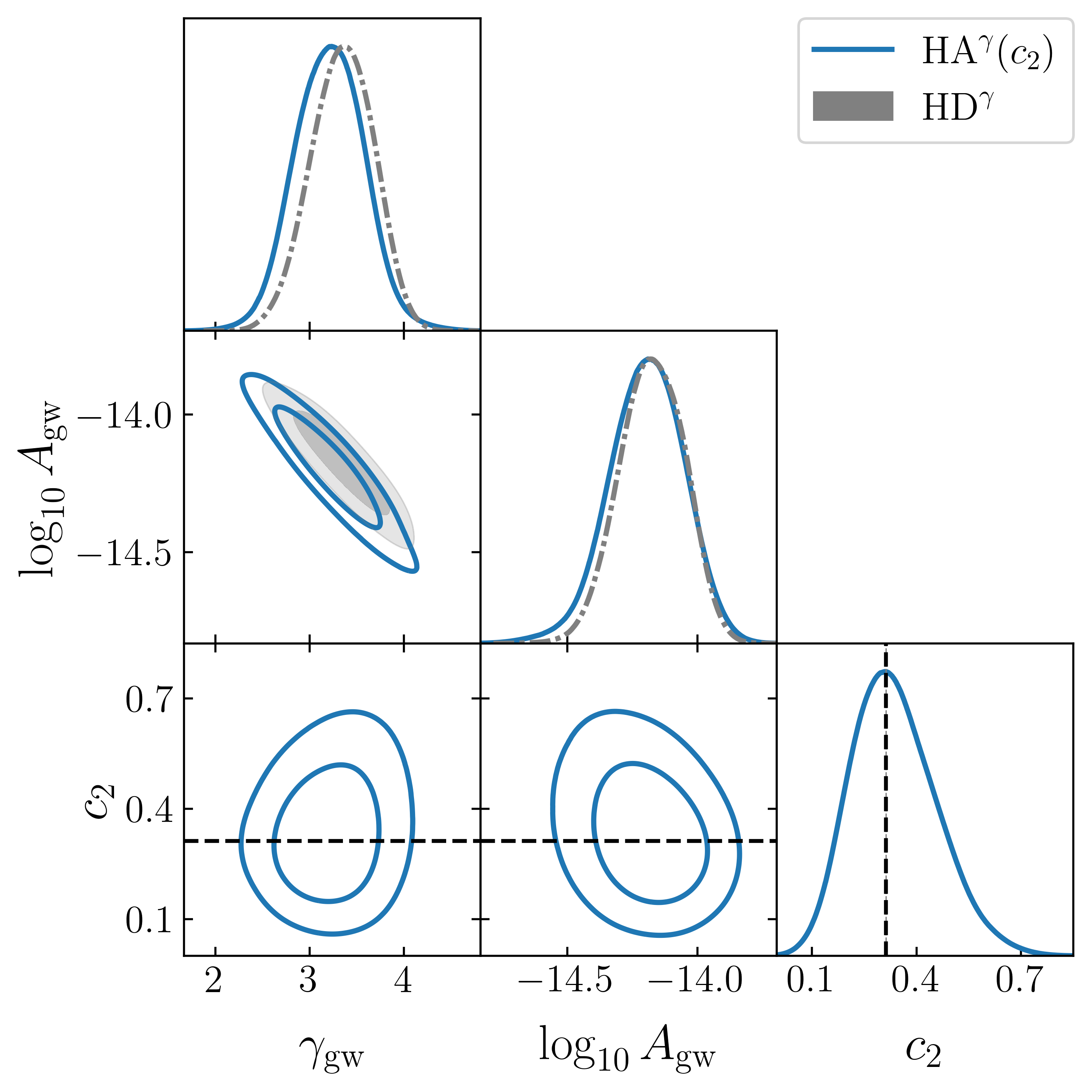
Figure 1: Marginalized 1D and 2D posterior distributions for quadrupole-only GWB harmonic analysis of the NG15 data set for the model $\text{HA}^{\gamma}(c_{2})$. The HD value for the quadrupole coefficient, $c_{2}^{\rm HD}=0.3125$ from Equation 8, is shown as the black dashed line. The GWB amplitude and spectral index from model $\text{HD}^{\gamma}$, which has angular correlations fixed to the theoretical HD values, are shown in gray.

3.3 Posterior Distributions

We show the marginalized 1D and 2D posterior distributions of the three GWB parameters from model $\text{HA}^{\gamma}(c_{2})$ when fit to the NG15 data set in Figure 1. The posterior distribution of $c_{2}$ is consistent with the theoretical HD value of the quadrupole correlation, $c_{2}^{\rm HD}=0.3125$ from Equation 8, denoted by the dashed line in Figure 1. The GWB amplitude and spectral index for an $\text{HD}^{\gamma}$ model, which has angular correlations fixed to the theoretical HD values, is shown in gray. We can see that the posterior distribution for $c_{2}$ is negligibly correlated with $\gamma_{\rm gw}$ and $\log_{10}A_{\rm gw}$.

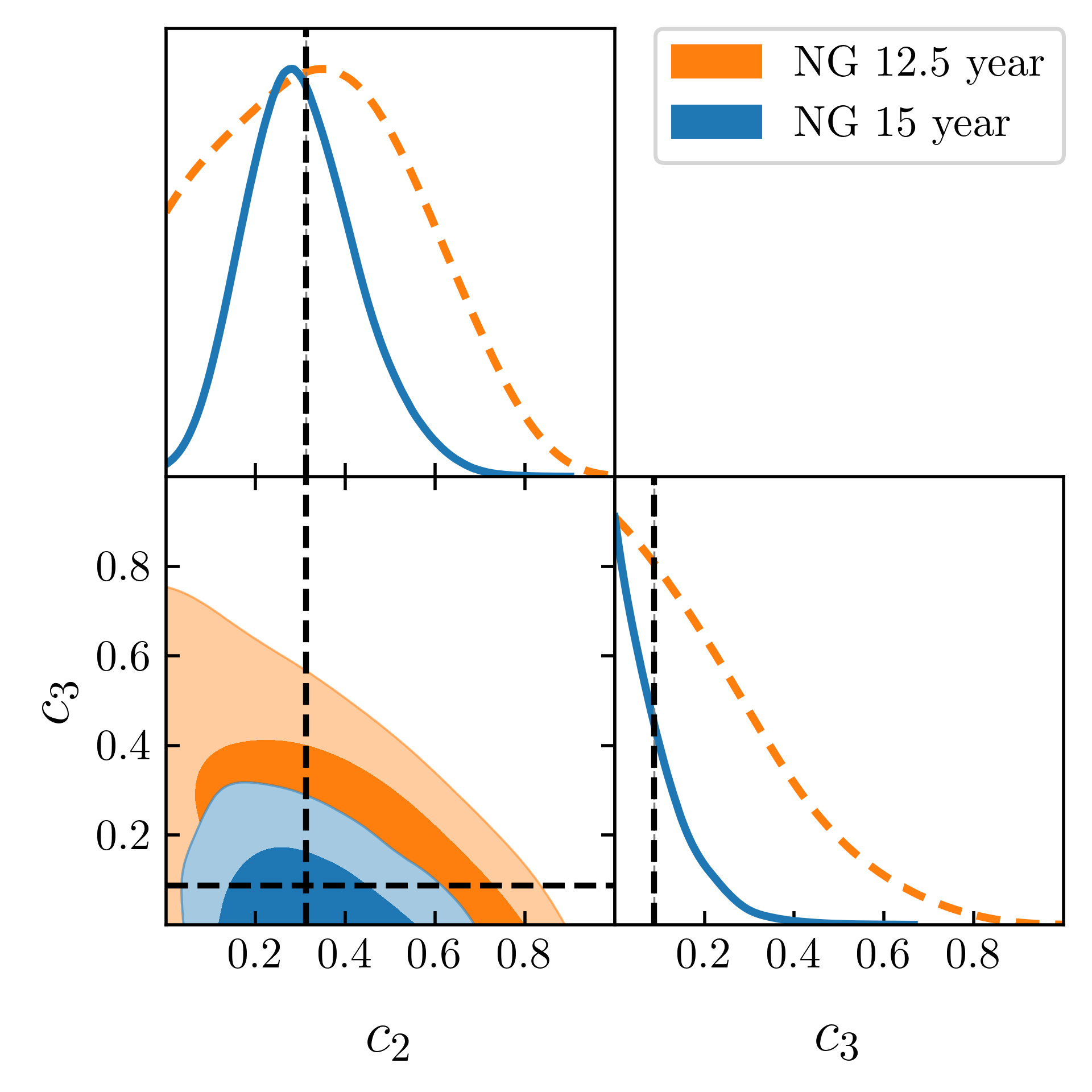
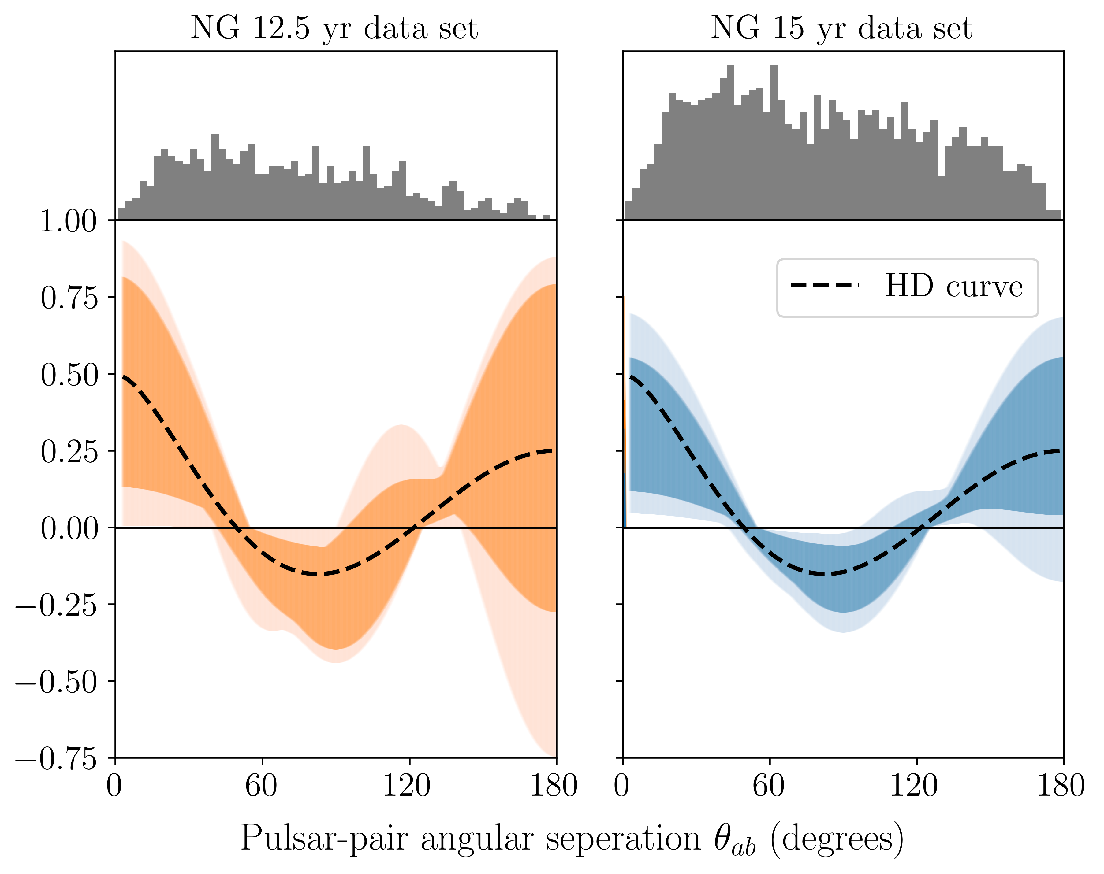
Figure 2: Left panel: Marginalized 1D and 2D posterior distributions of $c_{2}$ and $c_{3}$ for the harmonic analysis $\text{HA}^{\gamma}(c_{2},c_{3})$ of the NANOGrav 12.5 and 15 yr data sets. The dashed black lines show the HD value of each Legendre coefficient. Right panel: Reconstructed angular correlation function from the same $\text{HA}^{\gamma}(c_{2},c_{3})$ model with the NANOGrav 12.5 and 15 yr data sets. The dark- and light-shaded regions denote the 68% and 95% CL regions, respectively, from the marginalized 2D posterior distributions of the quadrupole and octupole parameters shown in the left panel. The dashed-black line is the HD curve, obtained from Equation 7. At the top of each plot, we provide a histogram of the pulsar-pair angular separations for these two NANOGrav data sets.

The quadrupole’s posterior distribution broadens as the number of Legendre coefficients in the model increases, as evident from Table 3. However, even for $\ell_{\rm max}=5$, the posterior distribution of $c_{2}$ is consistent with $c_{2}^{\rm HD}=0.3125$ and is non-zero at the 95% CL.

Using Equation 9, we can reconstruct the angular correlation function from the 68% and 95% contour regions of the marginalized 2D posterior distributions for $c_{2}$ and $c_{3}$. The right panel of Figure 2 shows these reconstructions from the harmonic analyses of the NG12.5 and NG15 data sets with model $\text{HA}^{\gamma}(c_{2},c_{3})$. The dark- and light-shaded regions denote the 68% CL and 95% CL regions, respectively. The dashed black line is the HD curve from Equation 6. At the top of each reconstructed angular correlation function, we provide a histogram of pulsar-pair angular separations for the two data sets.

For both the NG12.5 and NG15 data sets, the HD curve lies within the 68% contour region. We see a large reduction in the spread of the reconstructed angular-correlation function going from the NG12.5 data set to the NG15 data set, as expected given the change in quadrupole evidence between these data sets.

Figure 4 of Nay et al. (2024) provides approximate scaling relationships for the mean-to-standard deviation ratio of the Legendre coefficient’s marginalized 1D posterior distribution, as a function of the observation time and number of observed pulsars. For the quadrupole, this ratio is $\approx\!\!2.5$ in the NG15 data set, which is near the minimum value where the scaling relationships from Nay et al. (2024) begin to apply. For multipoles $\ell\geq 3$, this ratio is $\approx 1$ in all analyses.

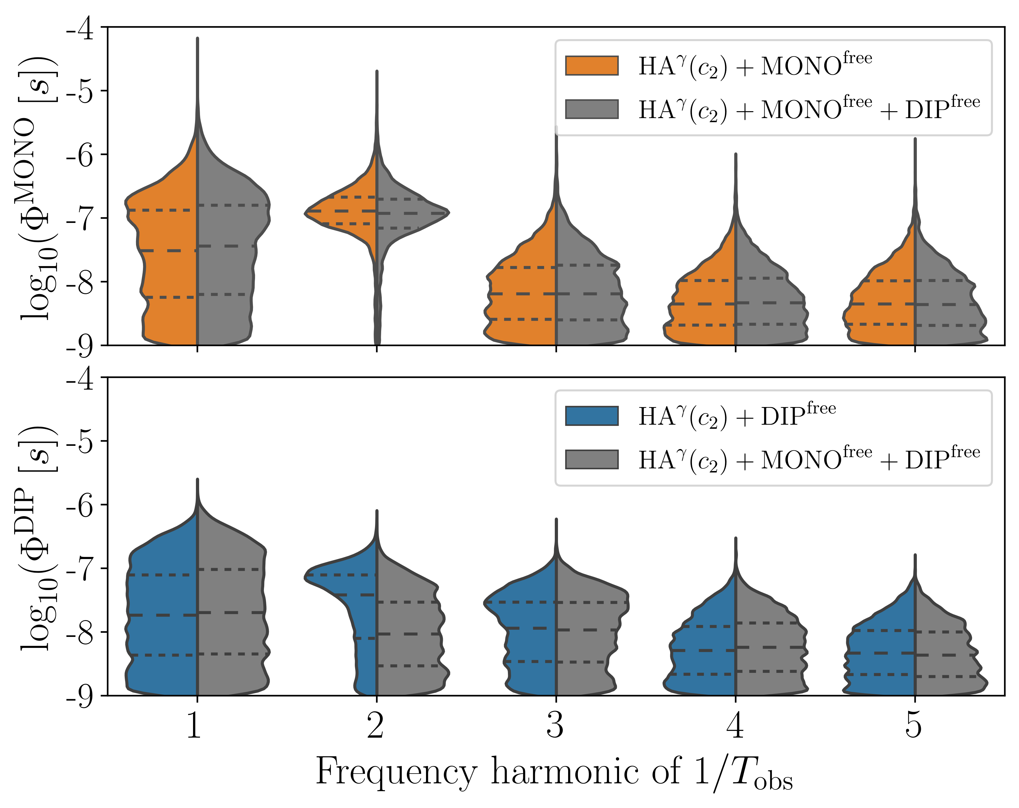
Figure 3: Marginalized 1D posterior distributions for the monopole (top plot) and dipole (bottom plot) free-spectrum parameters $\log_{10}\Phi_{i}$ of the first five frequency components $f_{i}=i/T_{\rm obs}$ where $i=1,...,5$. The green (right-hand) portion of the split violin plots show the results from a model that include both monopole and dipole free-spectrum models. For the NG15 data set, $T_{\rm obs}=16.03$ years, which gives frequency components as multiples of $\approx\!\!2$ nHz.

3.4 Monopole and Dipole Correlations

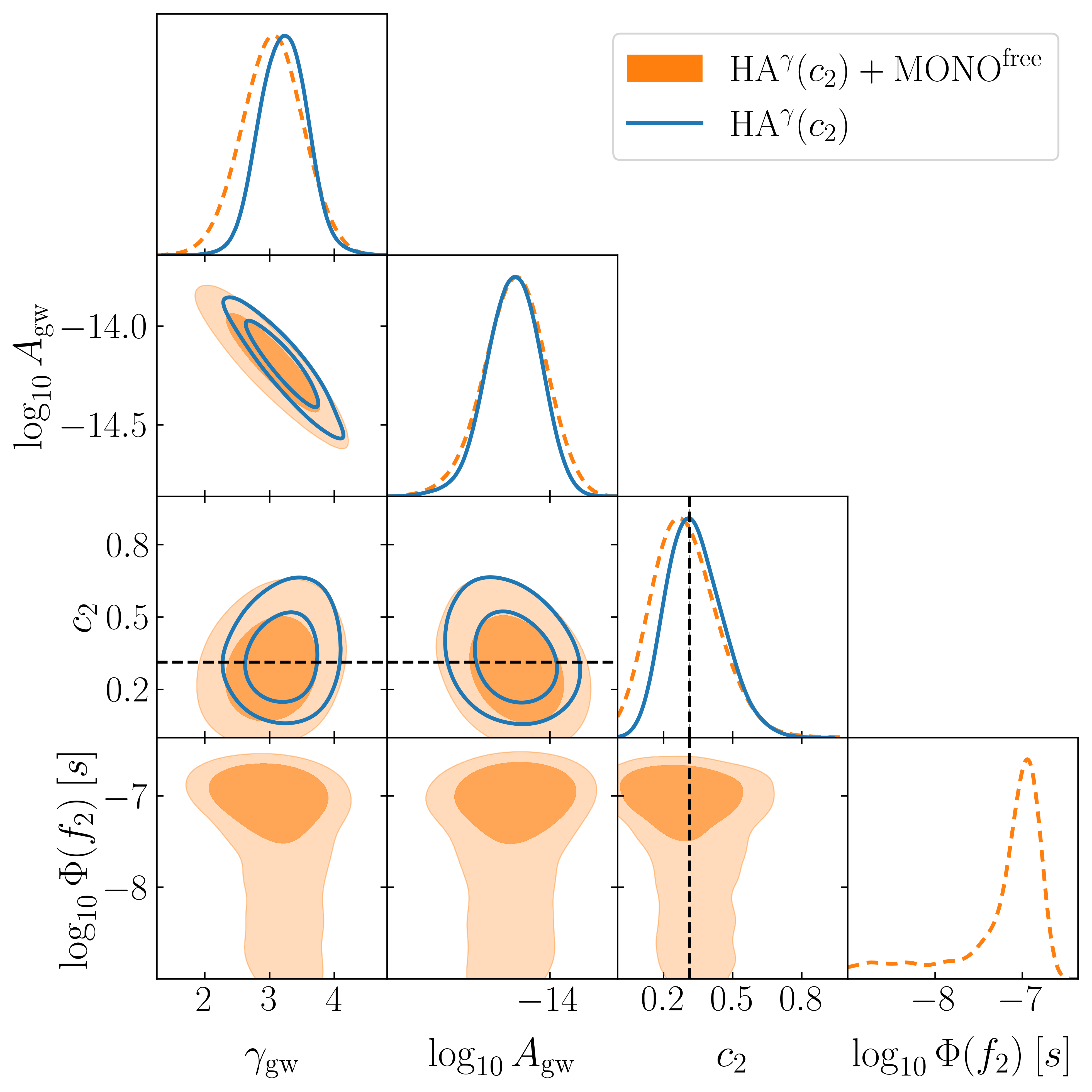
Figure 4: Marginalized 1D and 2D posterior distributions for a GWB analysis with monopole and quadrupole coefficients for the model $\text{HA}^{\gamma}(c_{2})+\text{MONO}^{\rm free}$ (shown as orange regions and dotted-orange curves), overlaid with a quadrupole-only GWB analysis for the model $\text{HA}(c_{2})$ (shown as solid blue curves). The monopole free-spectrum parameter $\log_{10}\Phi$ is associated with the second frequency bin ($f_{2}=2/T_{\rm obs}\approx 4\;\text{nHz}$). The full model includes monopole free-spectrum parameters from the $1$st through $5$th frequency bins. The dashed black line shows the HD value of the quadrupole coefficient.

To search for other possible correlations in the data, we add a monopole free-spectrum model ($\text{MONO}^{\rm free}$), dipole free-spectrum model ($\text{DIP}^{\rm free}$), or combination of both to GWB harmonic analysis model $\text{HA}^{\gamma}(c_{2})$. The violin plots in Figure 3 show the free-spectrum monopole and dipole models have power in the second frequency bin, $2/T_{\rm obs}\!\approx\!4\;\text{nHz}$. We isolate this effect to the $\text{MONO}^{\rm free}$ model: even though a $\text{DIP}^{\rm free}$ model has some power in the second frequency bin, the $\text{MONO}^{\rm free}+\text{DIP}^{\rm free}$ model shows the data prefers monopolar power in the second harmonic and no dipolar power in any harmonic. This result is consistent with other NANOGrav 15-year data set analysis results (e.g., see Figure 6 of NG15).

Figure 4 shows the marginalized 1D and 2D posterior distributions for model $\text{HA}^{\gamma}(c_{2})+\text{MONO}^{\rm free}$. Note that although they are present in the analysis, we leave out all other frequency bins except the second, since this is the only bin that has a non-zero posterior distribution. We overlay model $\text{HA}^{\gamma}(c_{2})$ in Figure 4 to show the effects on the harmonic analysis from including monopolar power in the model. This figure shows that when we include a monopole correlation, there is a reduction in the evidence for quadrupole correlations. Specifically, the Savage-Dickey Bayes factor for parameter $c_{2}$ is reduced from 90 [model $\text{HA}^{\gamma}(c_{2})$] to 5 [model $\text{HA}\gamma(c_{2})+\text{MONO}^{\rm free}$].

4 Comparison with previous work

Given the importance of the shape of the angular correlations, several methods have been used in the literature to extract angular information from the PTA data. The most common is to use a minimum variance estimator, known as the optimal statistic (OS), in order to either compute the angular correlations within a set of angular bins (Anholm et al., 2009; Demorest et al., 2013; Chamberlin et al., 2015; Vigeland et al., 2018). More recently, a generalization of the OS has been developed (Sardesai et al., 2023): the MCOS allows for multiple correlations to be simultaneously fit to the data. In NG15 the MCOS is used to estimate the amplitude of a Legendre polynomial expansion of the angular correlation function. Finally, in both NG12.5 and NG15, a splined angular correlation function is fit to the data, with knots placed over seven spline-knot positions (Taylor et al., 2013). The choice of seven spline-knot positions is based on features of the HD curve.

The MCOS constraints on the amplitude of the Legendre polynomials is closest to the analyses presented here. As shown in Figure 7 of NG15, the amplitude for the quadrupole, $A_{2}=A_{\rm gw}^{2}c_{2}$, is significantly non-zero, and the monopole, $A_{0}=A_{\rm gw}^{2}c_{0}$, has a relatively small amplitude but is also significantly non-zero. However, the significance of these non-zero multipoles is notably larger than what we have found here.

To understand this difference, we need to better understand the limitations of the MCOS analysis. The MCOS analysis presented in NG15 provides a minimum variance estimator of a parameterization of the auto-correlations for a fixed model of the auto-correlations, under the approximation of the weak signal limit (where the inverse of the pulsar covariance is assumed to be dominated by intrinsic noise), and does not include correlations between different pairs of pulsars arising from the fact that they measure the same gravitational wave background.

The full uncertainty in the MCOS comes from two distinct sources: one is the variance in the estimator, and the other is the uncertainty in the parameter values that model the auto-correlations (such as $A_{\rm gw}$ and the intrinsic red noise parameters). A method to marginalize over the uncertainty in the auto-correlations was presented in Vigeland et al. (2018) and used to compute the posterior distributions in Figure 7 of NG15. However, the estimator uncertainty is of a similar size as the uncertainty from the marginalization. Recently, Gersbach et al. (2024) proposed “uncertainty sampling” as a way to consistently combine both of these sources of uncertainty, but we stress that the error bars in Figure 7 of NG15 do not include the uncertainty in the estimator itself.

In addition to this, the assumption of a weak signal already breaks down for the NG15. Thus, the uncertainty in the MCOS is inherently an underestimate of the true uncertainty in the shape of the angular cross-correlations (Gersbach et al., 2024). Neglecting the pulsar-pair cross-correlations can underestimate the uncertainty by $20-40\%$ (Agazie et al., 2023a).

To directly compare the MCOS results with our work, we show the results of an analysis that includes the monopole, $c_{0}$, dipole, $c_{1}$, and quadrupole, $c_{2}$, in the solid curves in Figure 5. It is important to note that the harmonic analysis approach requires Legendre coefficients to be positive (given that the angular power spectrum is positive) and the sum of Legendre coefficients to be less than 1 (to maintain a positive definite GWB covariance matrix), whereas there is no constraint on the prior range of the $c_{\ell}$ coefficients in the MCOS approach. We only show positive values for the MCOS results for simplicity. The gray lines and contours show the MCOS posteriors when only accounting for the uncertainty in the auto-correlations, whereas the orange lines and contours include both uncertainty in the auto-correlations as well as the estimator uncertainty, following the proscription outlined in Gersbach et al. (2024). The blue contours show the result of the harmonic analysis presented here. In order to cast the MCOS results in terms of the multipoles, we re-scale the MCOS values by the value of $A^{2}_{\rm gw}$ obtained from the same point in the ${\rm CURN}^{\gamma}$ analysis chain.

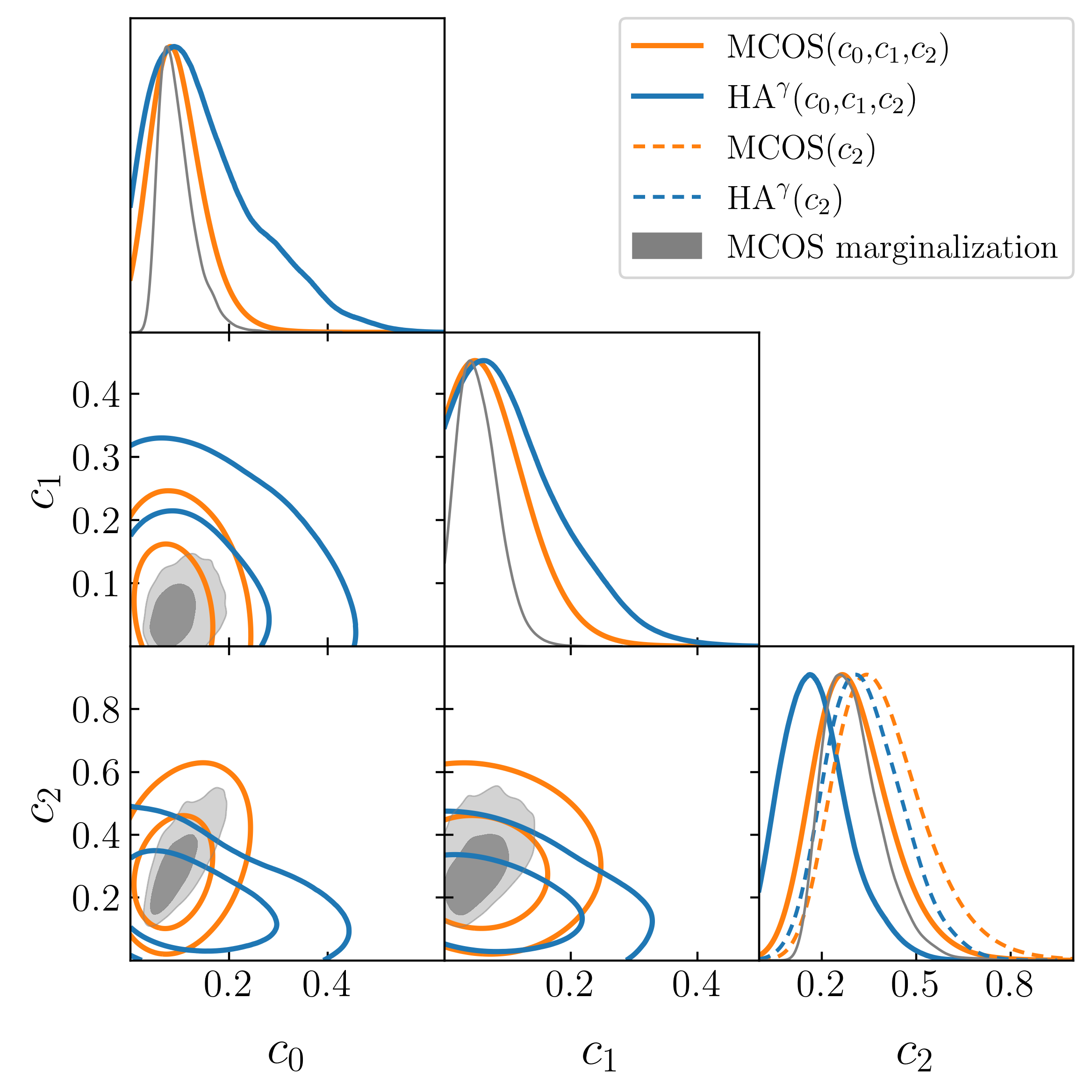
Figure 5: Marginalized 1D and 2D posterior distributions of frequentist MCOS and Bayesian harmonic analysis models with parameters $c_{0}$, $c_{1}$, and $c_{2}$. The gray curves show the MCOS analysis that appears in NG15. The uncertainty in this analysis solely comes from marginalizing over the ${\rm CURN}^{\gamma}$ parameters. The organge curves show the MCOS results when marginalizing over both the ${\rm CURN}^{\gamma}$ parameters and the estimator uncertainty, as outlined in (Gersbach et al., 2024). We do not include pulsar-pair covariance uncertainty for the MCOS results. The blue curves show the results of a harmonic analysis. The additional dashed curves in the 1D marginalized constraints on $c_{2}$ show $c_{2}$-only analyses, as indicated in the figure legend.

In Figure 5, we also overlay the MCOS and harmonic analysis marginalized 1D posterior distribution for a $c_{2}$-only model, shown as dashed curves. We see that the monopole coefficient has a larger impact on the posterior of the quadrupole for the harmonic analysis, compared to the MCOS approach. This is due to the fact that, as evident in the figure, the MCOS shows a positive correlation between $c_{0}$ and $c_{2}$, whereas the harmonic analysis shows a slight negative correlation. Intuitively, we expect the correlation to be negative: to keep the overall amplitude of the cross-correlations approximately constant, an increase in one of these coefficients would have to be accompanied by a decrease in the other.

We stress that the harmonic analysis presented here does not suffer from any of the issues identified for the MCOS: the harmonic analysis directly utilizes the PTA likelihood and does not make any assumptions about the relative amplitude of the cross-correlations, and the posterior distributions automatically take into account all sources of uncertainty.

Finally, we note that the MCMC spline analysis discussed in §3 of NG15 (and shown in Figure 6) provides similar information to our constraints on the multipoles. Just as in the harmonic analysis, the spline analysis fixes the correlation at $\theta_{ab}=0$ to unity, effectively separating the auto-correlations from the cross-correlations (Taylor et al., 2013). Since there are seven spline knots, we compare the spline analysis to the harmonic analysis ${\rm HA}^{\gamma}(c_{0},\dots,c_{6})$. In addition to having the same number of additional parameters, this harmonic analysis models variations in the correlations on the same angular scales. We show a comparison between these analyses in Figure 6. Both methods are consistent with one another and indicate that most of the evidence for non-zero angular-correlations comes from pulsar pairs separated by $\lesssim 30^{\circ}$.

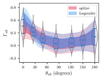
Figure 6: A comparison between constraints on the angular correlation function using a binned function (Taylor et al., 2013) (gray violins and red band) and the Legendre polynomial expansion ${\rm HA}^{\gamma}(c_{0},\dots c_{6})$ (Nay et al., 2024). The bands were constructed by drawing a large number of samples from the respective MCMCs and then computing the 1 and 2 $\sigma$ regions as a function of angular separation. The dashed black curve is the HD function.

5 Discussion and Conclusions

In this paper we extend the work of NG15 to further characterize the angular correlations in the NANOGrav 15-year data set using the harmonic analysis method from Nay et al. (2024). Our results show the Bayesian evidence for quadrupole-only correlation models are consistent with the evidence for the HD model found in NG15. We do not see evidence for multipoles higher than the quadrupole. We find the HD value of the quadrupole coefficient falls within the 68% CL of the measured quadrupole’s marginalized 1D posterior distribution, $c_{2}/c_{2}^{\rm HD}=1.088^{+0.32}_{-0.45}$. We reconstruct the angular correlation function from the posterior distributions for $c_{2}$ and $c_{3}$ and find the measurements are consistent with the angular correlations of the HD curve.

We show the large jump in quadrupole evidence between the NG12.5 and NG15 data sets is primarily due to the increase in the observation time, which is consistent with a GWB power law that has increasing strength at lower frequencies. This result is consistent with the expected scaling of the mean-to-standard deviation ratio of the quadrupole with time versus number of pulsars found in Nay et al. (2024). The current mean-to-standard deviation ratio of the octopole is $\sim 1$, and using the scaling found in Nay et al. (2024), we expect to have a mean-to-standard deviation ratio $\simeq 3$ within roughly 10 years.

Previous work in determining the shape of the measured angular correlations have either used a binned estimator of the correlations between pairs of pulsars (MCOS) or placed constraints on a spline parameterization of the angular correlations. Both of these approaches give broadly similar results to what we have found but also present some challenges when trying to interpret them. In particular, the MCOS results presented in NG15 neglect cross-correlations between different pairs of pulsars, leading to an underestimate of the resulting uncertainty, and constraints on the amplitude of the knots of the spline analysis are highly correlated with one another. We note that recent work on improving the frequentest estimator has included all pulsar cross-correlations, but that this has yet to be applied to providing constraints on the shape of the angular correlations (Gersbach et al., 2024).

When we include a monopole free-spectrum model in our harmonic analysis, the evidence of the quadrupole correlation is reduced by more than an order of magnitude due to the presence of a monopolar signal at $\approx\!\!4$ nHz, which has been investigated in detail. Clock errors can cause monopole correlations (Tiburzi et al., 2016; Arzoumanian et al., 2020), but extensive investigations by NANOGrav have shown no evidence of this type of systematic error (see discussion in §5.3 of NG15). Other possible explanations include GWs from an individual SMBHB source (Agazie et al., 2023d), ultralight dark matter (Afzal et al., 2023), and additional or alternate GW polarization modes (Agazie et al., 2024). To date, none of these additional investigations have been able to explain the source of the monopolar signal. As stated in NG15, if this monopolar signal is due to an astrophysical or cosmological source, then its persistence in future data sets will help determine the source of the signal. We also note that, to date, it is unclear whether the other PTA data sets are consistent with this monopolar signal, and we leave such an analysis to future work.

Our choice of parameterizing the angular correlations though Legendre polynomials is not unique—any set of complete functions can be used. For example it is possible to develop a set of functions which are statistically uncorrelated with the HD function (often referred to as “principal components”) (Madison, 2024). An analysis that uses these functions may be better suited to more clearly identify potential deviations from the expected angular correlations. However, given that the expected angular power spectrum is predominantly quadrupolar, a Legendre polynomial expansion is the natural choice when assessing the Bayesian evidence for angular correlations.

As our PTA data sets improve, it will be imperative to have multiple techniques to characterize the frequency and angular information contained within them. A confirmation of the standard expectations will lend credence to the interpretation that the GWB observed by PTAs is generated by a cosmological collection of SMBHBs generating tensor GWs that propagate at the speed of light. Even within this paradigm, we expect deviations due to the fact that the SMBHBs form a finite population that cluster on cosmological scales. Deviations from the standard expectations may provide evidence for unexpected dynamics in the SMBHB population, modifications to GR, and/or the presence of exotic GW sources such as cosmic strings or early universe phase transitions [see, e.g., Afzal et al. (2023)]. The confirmation that the currently measured angular correlations in the NG15 data set is largely consistent with standard expectations—though with hints of a possible monopole—is just a first step into a very exciting future.

References

- Afzal et al. (2023) Afzal, A., Agazie, G., Anumarlapudi, A., et al. 2023, The Astrophysical Journal Letters, 951, L11, doi: 10.3847/2041-8213/acdc91
- Agazie et al. (2023a) Agazie, G., Anumarlapudi, A., Archibald, A. M., et al. 2023a, The Astrophysical Journal Letters, 951, L8, doi: 10.3847/2041-8213/acdac6
- Agazie et al. (2023b) Agazie, G., et al. 2023b, Astrophys. J. Lett., 952, L37, doi: 10.3847/2041-8213/ace18b
- Agazie et al. (2023c) —. 2023c, Astrophys. J. Lett., 951, L10, doi: 10.3847/2041-8213/acda88
- Agazie et al. (2023d) —. 2023d, Astrophys. J. Lett., 951, L50, doi: 10.3847/2041-8213/ace18a
- Agazie et al. (2024) —. 2024, Astrophys. J. Lett., 964, L14, doi: 10.3847/2041-8213/ad2a51
- Ali-Haïmoud et al. (2020) Ali-Haïmoud, Y., Smith, T. L., & Mingarelli, C. M. F. 2020, Phys. Rev. D, 102, 122005, doi: 10.1103/PhysRevD.102.122005
- Allen et al. (2023) Allen, B., Dhurandhar, S., Gupta, Y., et al. 2023. https://arxiv.org/abs/2304.04767
- Anholm et al. (2009) Anholm, M., Ballmer, S., Creighton, J. D. E., Price, L. R., & Siemens, X. 2009, Phys. Rev. D, 79, 084030, doi: 10.1103/PhysRevD.79.084030
- Anholm et al. (2009) Anholm, M., Ballmer, S., Creighton, J. D. E., Price, L. R., & Siemens, X. 2009, Phys. Rev. D, 79, 084030, doi: 10.1103/PhysRevD.79.084030
- Antoniadis et al. (2023) Antoniadis, J., et al. 2023, Astron. Astrophys., 678, A50, doi: 10.1051/0004-6361/202346844
- Arzoumanian et al. (2020) Arzoumanian, Z., et al. 2020, Astrophys. J. Lett., 905, L34, doi: 10.3847/2041-8213/abd401
- Arzoumanian et al. (2021) —. 2021, Astrophys. J. Lett., 923, L22, doi: 10.3847/2041-8213/ac401c
- Boddy et al. (2022) Boddy, K. K., et al. 2022, JHEAp, 35, 112, doi: 10.1016/j.jheap.2022.06.005
- Caldwell et al. (2022) Caldwell, R., et al. 2022, Gen. Rel. Grav., 54, 156, doi: 10.1007/s10714-022-03027-x
- Chamberlin et al. (2015) Chamberlin, S. J., Creighton, J. D. E., Siemens, X., et al. 2015, Phys. Rev. D, 91, 044048, doi: 10.1103/PhysRevD.91.044048
- Chamberlin & Siemens (2012) Chamberlin, S. J., & Siemens, X. 2012, Phys. Rev. D, 85, 082001, doi: 10.1103/PhysRevD.85.082001
- Cornish et al. (2018) Cornish, N. J., O’Beirne, L., Taylor, S. R., & Yunes, N. 2018, Phys. Rev. Lett., 120, 181101, doi: 10.1103/PhysRevLett.120.181101
- Demorest et al. (2013) Demorest, P. B., Ferdman, R. D., Gonzalez, M. E., et al. 2013, ApJ, 762, 94, doi: 10.1088/0004-637X/762/2/94
- Detweiler (1979) Detweiler, S. L. 1979, Astrophys. J., 234, 1100, doi: 10.1086/157593
- Dickey (1971) Dickey, J. M. 1971, The Annals of Mathematical Statistics, 42, 204. http://www.jstor.org/stable/2958475
- Ellis & van Haasteren (2017) Ellis, J., & van Haasteren, R. 2017, jellis18/PTMCMCSampler: Official Release, 1.0.0, Zenodo, doi: 10.5281/zenodo.1037579
- Ellis et al. (2020) Ellis, J. A., Vallisneri, M., Taylor, S. R., & Baker, P. T. 2020, ENTERPRISE: Enhanced Numerical Toolbox Enabling a Robust PulsaR Inference SuitE, v3.0.0, Zenodo, doi: 10.5281/zenodo.4059815
- Gair et al. (2014) Gair, J., Romano, J. D., Taylor, S., & Mingarelli, C. M. F. 2014, Phys. Rev. D, 90, 082001, doi: 10.1103/PhysRevD.90.082001
- Gelman & Rubin (1992) Gelman, A., & Rubin, D. B. 1992, Statist. Sci., 7, 457, doi: 10.1214/ss/1177011136
- Gersbach et al. (2024) Gersbach, K. A., Taylor, S. R., Meyers, P. M., & Romano, J. D. 2024. https://arxiv.org/abs/2406.11954
- Green et al. (2022) Green, D., et al. 2022. https://arxiv.org/abs/2209.06854
- Hellings & Downs (1983) Hellings, R. W., & Downs, G. S. 1983, The Astrophysical Journal Letters, 265, L39, doi: 10.1086/183954
- Hobbs et al. (2012) Hobbs, G., Coles, W., Manchester, R. N., et al. 2012, Monthly Notices of the Royal Astronomical Society, 427, 2780, doi: 10.1111/j.1365-2966.2012.21946.x
- Hobbs et al. (2019) Hobbs, G., Guo, L., Caballero, R. N., et al. 2019, Monthly Notices of the Royal Astronomical Society, 491, 5951, doi: 10.1093/mnras/stz3071
- Hotinli et al. (2019) Hotinli, S. C., Kamionkowski, M., & Jaffe, A. H. 2019, Open J. Astrophys., 2, 8, doi: 10.21105/astro.1904.05348
- Jeffreys (1998) Jeffreys, H. 1998, The theory of probability (OuP Oxford)
- Johnson et al. (2023) Johnson, A. D., et al. 2023. https://arxiv.org/abs/2306.16223
- Lee et al. (2008) Lee, K. J., Jenet, F. A., & Price, R. H. 2008, ApJ, 685, 1304, doi: 10.1086/591080
- Madison (2024) Madison, D. R. 2024. https://arxiv.org/abs/2410.23381
- Maggiore (2018) Maggiore, M. 2018, Gravitational Waves. Vol. 2: Astrophysics and Cosmology (Oxford University Press)
- Matsakis et al. (1997) Matsakis, D. N., Taylor, J. H., & Eubanks, T. M. 1997, A&A, 326, 924
- Mingarelli & Casey-Clyde (2022) Mingarelli, C. M. F., & Casey-Clyde, J. A. 2022, Science, 378, 592, doi: 10.1126/science.abq1187
- Mingarelli et al. (2013) Mingarelli, C. M. F., Sidery, T., Mandel, I., & Vecchio, A. 2013, Phys. Rev. D, 88, 062005, doi: 10.1103/PhysRevD.88.062005
- Nay et al. (2024) Nay, J., Boddy, K. K., Smith, T. L., & Mingarelli, C. M. F. 2024, Phys. Rev. D, 110, 044062, doi: 10.1103/PhysRevD.110.044062
- Phinney (2001) Phinney, E. S. 2001. https://arxiv.org/abs/astro-ph/0108028
- Qin et al. (2019) Qin, W., Boddy, K. K., Kamionkowski, M., & Dai, L. 2019, Phys. Rev. D, 99, 063002, doi: 10.1103/PhysRevD.99.063002
- Reardon et al. (2023) Reardon, D. J., et al. 2023, Astrophys. J. Lett., 951, L6, doi: 10.3847/2041-8213/acdd02
- Roebber (2019) Roebber, E. 2019, Astrophys. J., 876, 55, doi: 10.3847/1538-4357/ab100e
- Roebber & Holder (2017) Roebber, E., & Holder, G. 2017, Astrophys. J., 835, 21, doi: 10.3847/1538-4357/835/1/21
- Sardesai et al. (2023) Sardesai, S. C., Vigeland, S. J., Gersbach, K. A., & Taylor, S. R. 2023, Phys. Rev. D, 108, 124081, doi: 10.1103/PhysRevD.108.124081
- Sazhin (1978) Sazhin, M. V. 1978, Soviet Ast., 22, 36
- Taylor et al. (2021) Taylor, S. R., Baker, P. T., Hazboun, J. S., Simon, J., & Vigeland, S. J. 2021, enterprise-extensions. https://github.com/nanograv/enterprise_extension
- Taylor & Gair (2013) Taylor, S. R., & Gair, J. R. 2013, Phys. Rev. D, 88, 084001, doi: 10.1103/PhysRevD.88.084001
- Taylor et al. (2013) Taylor, S. R., Gair, J. R., & Lentati, L. 2013, Phys. Rev. D, 87, 044035, doi: 10.1103/PhysRevD.87.044035
- Tiburzi et al. (2016) Tiburzi, C., Hobbs, G., Kerr, M., et al. 2016, Mon. Not. Roy. Astron. Soc., 455, 4339, doi: 10.1093/mnras/stv2143
- Vallisneri et al. (2020) Vallisneri, M., Taylor, S. R., Simon, J., et al. 2020, ApJ, 893, 112, doi: 10.3847/1538-4357/ab7b67
- Vigeland et al. (2018) Vigeland, S. J., Islo, K., Taylor, S. R., & Ellis, J. A. 2018, Phys. Rev. D, 98, 044003, doi: 10.1103/PhysRevD.98.044003
- Xu et al. (2023) Xu, H., et al. 2023, Res. Astron. Astrophys., 23, 075024, doi: 10.1088/1674-4527/acdfa5