Information scrambling and entanglement dynamics in Floquet Time Crystals

Abstract

We study the dynamics of out-of-time-ordered correlators (OTOCs) and entanglement of entropy as quantitative measures of information propagation in disordered many-body systems exhibiting Floquet time-crystal (FTC) phases. We find that OTOC spreads in the FTC with different characteristic timescales due to the existence of a preferred “quasi-protected” direction - denoted as $\ell$-bit direction - along which the spins stabilize their period-doubling magnetization for exponentially long times. While orthogonal to this direction the OTOC thermalizes as an usual MBL time-independent system (at stroboscopic times), along the $\ell$-bit direction the system features a more complex structure. The scrambling appears as a combination of an initially frozen dynamics (while in the stable period doubling magnetization time window) and a later logarithmic slow growth (over its decoherence regime) till full thermalization. Interestingly, in the late time regime, since the wavefront propagation of correlations has already settled through the whole chain, scrambling occurs at the same rate regardless of the distance between the spins, thus resulting in an overall envelope-like structure of all OTOCs, independent of their distance, merging into a single growth. Alongside, the entanglement entropy shows a logarithmic growth over all time, reflecting the slow dynamics up to a thermal volume-law saturation.

I Introduction

Similar to ordinary crystals, time crystals exhibit a high degree of structural order. While ordinary crystals derive their periodicity from the regular repetition of spatial elements, time crystals are an exotic, non-equilibrium state of matter in which the structure arises over time. Both are instances of spontaneous symmetry breaking: the breaking of spatial translation symmetry leads to the formation of crystals, while the breaking of time translation symmetry leads to the formation of time crystals.

Since quantum states in equilibrium have inherently time-independent observables, time-translation symmetry (TTS) arise more naturally in non-equilibrium settings. Indeed, in periodically driven systems, also known as Floquet dynamics, a broad class of models has been shown to break TTS [1]. In this case, although the system is periodically driven with a Hamiltonian of period T, $\hat{H}(t)=\hat{H}(t+T)$, it has observables $O(t)$ (e.g., spin magnetization) that exhibit subharmonic responses, i.e., $O(t)=O(t+nT)$ with $n>1$. Therefore, the system spontaneously breaks the TTS and exhibits a Floquet Time Crystal (FTC) phase.

In general a FTC has an ergodicity breaking mechanism in order to maintain its long-range time ordering, such as induced by disorder in many-body localization (MBL) [2, 3, 4, 5], long-range interactions [6, 7, 8, 9, 10, 11, 12, 13, 14], Stark effect [15, 16], many-body Scars [17, 18], dissipative dynamics  [19, 20, 21, 22, 23, 24, 25, 26, 27, 28, 29, 30], among others [31, 32, 33, 34, 35]. In this manuscript we focus on closed MBL periodically driven systems. The many-body localization resulting from strong disorder prevents the quantum system from absorbing the driving energy and heating to infinite temperatures. This new phase of matter has led to several experimental realizations on different platforms, including trapped atomic ions [36], nitrogen-vacancy centers in diamond [37], superconducting quantum processors [38, 39], spin-based quantum simulators [40], and others [41, 42]. Moreover, the use of time crystals for quantum applications has been a subject of growing interest recently, with promissing prospects as quantum sensors [43, 44, 45, 46, 47, 48, 49], complex network simulators [50], quantum engines  [51], among others [52, 53, 54].

In non-equilibrium settings, not only the dynamics of local observables is important, but also their correlations and more generally the propagation of information. Interactions can cause the spread of initially localized quantum information into the exponentially many degrees of freedom of the system, a process known as information scrambling [55, 56]. As a consequence, the scrambled information cannot be recovered by local measurements, leading to thermalization [57, 58, 59]. An unambiguous description of this scrambling process remains an open problem. One way to explore it is through out-of-time-ordered correlators  [60, 55], which can help define a quantum analog of the Lyapunov exponent found in classical chaos [61]. This applies to certain systems, typically those in a semi-classical limit or with a large number of local degrees of freedom, which obey a universal upper bound [62, 63, 64, 65].

Out-of-time-ordered correlators (OTOCs) allow us to measure the growth of operators. Consider two local operators, $\hat{W}$ and $\hat{V}$, in a one-dimensional spin chain. The idea is to study the spread of $\hat{W}(t)=e^{i\hat{H}t}\hat{W}e^{-i\hat{H}t}$ using another operator $\hat{V}$, which is a simple spin operator located at some distance $\ell$ from $\hat{W}$. This can be done by looking at the expectation value of the squared commutator:

$$C(\ell,t)=\left\langle[\hat{W}(t),\hat{V}]^{\dagger}[\hat{W}(t),\hat{V}]\right\rangle/2$$ (1)

Initially, this value will be zero for well-separated operators, but it will become significantly different from zero once $\hat{W}(t)$ has spread to the location of $\hat{V}$. In the special case where $\hat{W}$ and $\hat{V}$ are Hermitian and unitary, the squared commutator can be written as $C(\ell,t)=1-\text{Re}[\langle\hat{W}(t)\hat{V}\hat{W}(t)\hat{V}\rangle]$, with $F(t)=\langle\hat{W}(t)\hat{V}\hat{W}(t)\hat{V}\rangle$ showing explictly the out-of-time ordering nature of the operators. The growing interest in OTOCs has led to numerous experimental proposals and experiments aimed at measuring them [66, 67, 68, 69, 70, 71].

For systems with a geometrically local Hamiltonian that do not exhibit localized phase, $C(\ell,t)$ typically exhibits a ballistic growth [72, 73, 74, 75], leading to an emergent linear light cone with a butterfly velocity $v_{B}$, displaying in this way a rapid growth ahead of the wavefront and a saturation behind it at late times. On the other hand, the growth of $C(\ell,t)$ is severely suppressed in disordered system [76, 77]. In MBL phases [78, 79, 80, 81, 82], characterized by an extensive number of local integrals of motion, the $C(\ell,t)$ exhibits a logarithmic light cone [83, 84, 85, 86].

A different way to track the propagation of information is to examine the buildup of entanglement among the system constituents, which could be quantified by the entanglement entropy. In a quench system, starting from an unentangled product state, the entanglement entropy initially starts at zero and grows over time. In a thermal system, at late times, the subsystem’s density matrix approaches a mixed state, corresponding to a thermal state with a temperature set by the average energy of the initial state. In contrast, in a many-body localized (MBL) system, entanglement entropy grows slowly and saturates at exponentially late times relative to the system size  [87, 88, 89, 79].

In this manuscript, we study scrambling and correlation dynamics in a periodically driven disordered spin chain. Specifically, the model consists of interacting nearest-neighbor spins in a disordered chain subject to periodic global spin flips. The system exhibits both an FTC stabilized by MBL as well as a regular ergodic phase for varying its parameters. The scrambling and correlation dynamics over MBL and ergodic phases have been largely discussed in time-independent Hamiltonian systems, it is therefore natural to ask how does the presence of Floquet dynamics, and more specifically of TTS breaking, impacts the phenomenology.

Our study shows that the OTOC growth has different characteristic time scales in the FTC due to the existence of a preferred “quasi-protected” direction - so called $\ell$-bit direction. While orthogonal to it the OTOC thermalizes as an usual MBL system, along the localized $\ell$-bit axis the system features a slow scrambling with a combination of frozen dynamics and a later logarithmic slow growth till full thermalization. Interestingly, the late scrambling occurs at the same rate regardless of the distance between the spins, resulting in an overall envelope of all OTOCs independent of their distance. This peculiar behaviour can be interpreted by the fact that at late times the wavefront propagation of correlations has already settled through the whole chain. The entanglement entropy also features a logarithmically growth over all time, reflecting the slow dynamics till a thermal volume-law saturation.

The paper is structured as follows. We begin with introducing the model in Sec. II. In Sec. III, we present our results for the magnetization dynamics, OTOCs, and entanglement entropy at all time scales. We summarize and conclude with future direction in Sec. IV. In Appendix A we provide the analytics for the OTOC in absence of perturbative field.

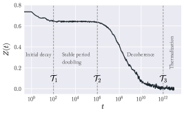
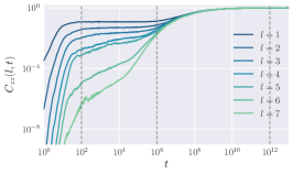
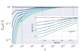
Figure 1: (Left) The dynamics of magnetization $Z(t)$ in the FTC phase, and its different characteristic time scales $\mathcal{T}_{i}$ (vertical dotted lines). The magnetization displays a period doubling plateau in the fully stable regime of the time crystal, which later slowly decoheres and thermalises at late times. We show the corresponding dynamics of OTOCs along the (center) $z$-direction ($C_{zz}(l,t)$) and (right) $x$-direction ($C_{xx}(l,t)$), for varying spin distances $l$. The inset-panel shows the dynamics within the regime $\mathcal{T}_{1}<t<\mathcal{T}_{2}$ in a semi-log scale in order to highlight the logarithmic growth of the OTOC, where the dotted curves are the fitted plots using the function $(\log t)^{a_{\alpha\beta}(l)}$. In all results we used $L=8$ spins and coupling parameters $J=1$, $h^{x}=0.2$, and $h^{z}=1$. The operator distances $l$ are always taken from the bulk of the spin chain to the edges (most distant spins).

II The Model

We consider a one-dimensional spin-$1/2$ chain with a Floquet unitary of the form

$$\hat{U}_{F}=\exp(-i\hat{H}_{0}T)\,\hat{U}_{K},\quad\hat{U}_{K}\equiv\exp\left(i\phi\sum_{i=1}^{N}\hat{\sigma}_{i}^{x}/2\right),$$ (2)

where $L$ is the number of spins in the chain, $T$ the period of the Floquet dynamics, $\phi$ the kicking phase and the Hamiltonian is defined as,

$$\hat{H}_{0}=\sum_{i}\left(J_{i}\hat{\sigma}_{i}^{z}\hat{\sigma}^{z}_{i+1}+h_{i}^{z}\hat{\sigma}^{z}_{i}+h^{x}_{i}\hat{\sigma}_{i}^{x}\right)$$ (3)

with $\hat{\sigma}_{i}^{\alpha}$ the Pauli operator for the $i$’th spin along the $\alpha=x,y,z$ direction. The couplings $J_{i},h_{i}^{z}$, and $h_{i}^{x}$ are uniformly chosen from $J_{i}\in[J/2,3J/2]$ , $h_{i}^{z}\in[0,h^{z}]$, $h_{i}^{x}\in[0,h^{x}]$. For strong enough disordered interaction ($J_{i}$) and in case of no kicking ($\phi=0$), the system evolves to an MBL state. In case of periodic kickings close to $\phi\backsimeq\pi$ the dynamics stabilizes a FTC phase [90]. The FTC displays a robust period doubling magnetization dynamics, which was observed in various experiments [37, 36, 40, 39, 38, 91].

III FTC dynamics

In this section, we show our results for the dynamics of magnetization, OTOCs, and entanglement entropy in the FTC phase. Their behaviour follow different growth/decay rates at corresponding characteristic time scales, which depend on the coupling parameters and system size, as we discuss in detail. In all our simulations we consider initial product states $\left[\cos\theta\lvert\uparrow\rangle+\sin\theta\lvert\downarrow\rangle\right]^{\otimes N}$, with $\theta=\pi/8$, open boundary conditions and average our results over $10^{3}$ disorder simulations.

III.1 Magnetization dynamics

The period doubling dynamics can be computed analytically in the simpler case of no transverse field $h^{x}=0$ and a kicking phase $\phi=\pi$, where $\hat{U}_{K}=\prod_{i}i\hat{\sigma}^{x}_{i}$ has the effect of perfectly flipping all the spins. In this case the Hamiltonian $\hat{H}_{\text{0}}$ is diagonal in eigenbasis ($\lvert\uparrow\rangle$ and $\lvert\downarrow\rangle$) of individual Pauli $\hat{\sigma}^{z}_{i}$ operator. Each eigenstate of the Hamiltonian $H_{\text{0}}$ can be written as $|s_{1}s_{2}\ldots\rangle\equiv|\{s_{i}\}\rangle$ with $s_{i}=\pm 1$, so that $\hat{\sigma}^{z}_{k}|\{s_{i}\}\rangle=s_{k}|\{s_{i}\}\rangle$. The action of the Floquet unitary $\hat{U}_{F}$ on a random initial product state is to flip each spin, i.e. $\hat{U}_{F}|\{s_{i}\}\rangle=e^{-iE(\{s_{i}\})T}\lvert\uparrow\downarrow\downarrow\uparrow\downarrow\cdots\rangle$ where $E(\{s_{i}\})$ is energy eigenvalue of state $|\{s_{i}\}$ associated with Hamiltonian $\hat{H}_{\text{0}}$. The magnetization $\langle\hat{\sigma}^{z}_{i}(t)\rangle$ oscillates with period $2T$, while the magnetization

$$Z(t)=(-1)^{t}\langle\hat{\sigma}^{z}_{i}(t)\rangle\text{sgn}\left(\langle\hat{\sigma}_{i}^{z}(0)\rangle\right)$$ (4)

takes a constant value. Most importantly, for large system sizes $N$ and disordered interactions $J_{i}$, the period doubling dynamics is stable under perturbations of the Floquet operator such as a non-zero transverse field $h^{x}$ or imperfect spin flip $\phi=\pi+\epsilon$ [2]. Therefore, the system breaks the time-translation symmetry stabilizing a FTC phase.

In the general case, the magnetization dynamics in FTCs for finite-system sizes can be described by different dynamical regimes. We illustrate them in Fig.(1)-(left panel). The magnetization exhibits in increasing order of time:

$\bullet\ \,0<t<\mathcal{T}_{1}$: a first initial spin relaxation leading to a decay in the magnetization. This first dynamical regime is general and roughly independent on the spin microscopic details, i.e., to an MBL/ergodic/FTC phase;

$\bullet\ \,\mathcal{T}_{1}<t<\mathcal{T}_{2}$: a stable period doubling dynamics till time $\mathcal{T}_{2}$, with all the spins now in a coherent dynamics due to kicking and MBL interactions. Due to MBL, the time scale for period doubling dynamics increases exponentially with the system size, $\mathcal{T}_{2}\sim e^{\beta N},\beta>0$, therefore persisting indefinitely in the macroscopic limit, $N\rightarrow\infty$.

$\bullet\ \,\mathcal{T}_{2}<t<\mathcal{T}_{3}$: for longer times, the spins now start to decohere among each other and the magnetization $Z(t)$ slowly decays. We find a logarithmic decay leading to a characteristic time scale exponentially long with the system size, $\mathcal{T}_{3}=e^{\beta^{\prime}N}$. In particular, for the chosen parameters, a time exponent even larger than the period doubling regime, with $\beta^{\prime}\approx 0.95>\beta\approx 0.43$.

$\bullet\ \,\mathcal{T}_{3}<t$: in the late time, the system has now thermalized, with a null net magnetization, $Z(t)\rightarrow 0$, and trivial dynamics.

III.2 Out-of-time-ordered correlator

We now turn our attention to the behavior of OTOCs (Eq. (1)). We consider the scrambling of local spin operators: $\hat{W}(0),\hat{V}\in\{\hat{\sigma}_{i}^{\alpha}\}$. In order to simplify the notation, we define

$$C_{\alpha\beta}(\ell,t)\equiv\frac{1}{2}\left\langle\left|[\hat{\sigma}_{\ell}^{\alpha}(t),\hat{\sigma}^{\beta}_{1}]\right|^{2}\right\rangle$$ (5)

where $\ell=1,...,N$, and $\alpha,\beta\in\{x,y,z\}$. We focus on $C_{xx}(\ell,t),C_{zz}(\ell,t)$ as these are representative of the main behaviors of the OTOC in the system.

In the case of a perfect spin-flip ($\phi=\pi$) with no transverse field ($h^{x}=0$), the local operators along the different directions remain local under the Floquet unitary. Therefore the OTOC for distant spins is constant over time (see Appendix A). This is a fine-tuning point of the model (limit of vanishing correlation length), for which there is no scrambling, and it is not representative of the general behavior.

In the general FTC case, the scrambling dynamics display different characteristic time scales $\mathcal{T}_{i}$, whose main features are strongly influenced by the spin directions - see Fig.(1) - as we discuss below.

$\bullet\,\,0<t<\mathcal{T}_{1}$: the initial OTOC growth arises due to the spins initial relaxation - similar to magnetization dynamics - and it is independent on the underlying non-equilibirum phase;

$\bullet\,\,\mathcal{T}_{1}<t<\mathcal{T}_{2}$: despite in a stable period doubling magnetization, the OTOC has a slow growth in this regime. Its main behavior (apart from small corrections, discussed later) is similar to an MBL-like dynamics. I.e., its growth resembles those of a quench dynamics in a time-independent MBL spin system [92, 93]. After the initial transient time $\mathcal{T}_{1}$, the OTOC shows a logarithmically scrambling of information, with

$$C_{\alpha\beta}(\ell,t)\sim A_{\alpha\beta}(\ell)\log(t)^{a_{\alpha\beta}(\ell)},$$ (6)

where $A_{\alpha\beta}(\ell)\sim e^{-v_{\alpha\beta}\ell}$ - see inset of Fig.(1)-(right panel). The exponents $a_{\alpha\beta}(\ell),v_{\alpha\beta}(\ell)$ are non-universal, depending on the distance and system interactions. A few observations are in order. While both $C_{xx}(\ell,t)$ and $C_{zz}(\ell,t)$ show a slow growth, one clearly notice that the scrambling along the $x$-direction is much larger (by orders of magnitude) than the one along the $z$-direction. Indeed, while closer spins ($\ell\lesssim 3$) $C_{xx}(\ell,t)$ may already get fully scrambled in this time window, $C_{zz}(\ell,t)$ has generally rather small values, remaining close to rough plateau’s depending on their spin distances. These small values arise due to the (period doubled) conservation of the $z$-magnetization, which causes only a small part of $\hat{\sigma}_{i}^{z}$ to scramble, leaving the most of it protected during the dynamics. On the other hand, the magnetization along the $x$-direction has no protection or stability in the FTC, i.e., it is vanishingly small even within the period doubling time regime, with expectation values resembling those of a high temperature state, therefore leading to a larger (in magnitude) scrambled $\hat{\sigma}_{i}^{x}$ spin operator.

Alternatively, one could also understand this regime by recalling an $\ell$-bit phenomenological model for MBL-like dynamics [94, 95, 96, 97, 98]. The picture assumes the existence of local integrals of motion along a preferred direction, denoted as $\ell$-bit operators, $\hat{\tau}_{i}^{z}$. In the limit of infinite localization, one expects the local spin operators to be roughly aligned to the integral of motion, as e.g. in the simplest FTC case with perfect spin-flip ($\phi=\pi$) and no transverse field ($h^{x}=0$), where we easily identify $\hat{\sigma}_{i}^{z}=\hat{\tau}_{i}^{z}$. On the general case though (not infinite localization), the spin operators $\hat{\sigma}_{i}^{\alpha}$ have an overlap both into more distant $\ell$-bit operators ($\hat{\tau}_{j\neq i}^{\alpha}$) as well as onto different orthogonal $\hat{\tau}_{j}^{x}$ and $\hat{\tau}_{j}^{y}$ directions, which are not integrals of motion. Specifically,

$$\hat{\sigma}_{i}^{\alpha}=\sum_{j,\beta}{c}_{j,\beta}^{[i,\alpha]}\hat{\tau}_{j}^{\beta}+\sum_{jk}{c}_{jk,\beta\gamma}^{[i,\alpha]}\hat{\tau}_{j}^{\beta}\hat{\tau}_{k}^{\gamma}+...$$ (7)

with the coefficients ${c}_{...}^{[i,\alpha]}$ exponentially localized around the $i$’th position, corresponding to the overlap into the new locally deformed $\{\hat{\tau}_{i}^{\alpha}\}$ basis. The last “$\cdots$” term in the equation represents possible higher order products of $\ell$-bit operators. Therefore, as long as the spin operator has an overlap into an orthogonal direction - $\hat{\tau}_{j}^{x,y}$ - part of it scrambles, and this explains the difference between $C_{xx}(\ell,t)$ and $C_{zz}(\ell,t)$ behaviors. Both $\hat{\sigma}_{i}^{z}$ and $\hat{\sigma}_{i}^{x}$ spin operators have, in general, an overlap onto the the orthogonal $\ell$-bit operators. However, while spin $\hat{\sigma}_{i}^{z}$ has a vanishing small overlap, which decreases with the localization strength, $\hat{\sigma}_{i}^{x}$ has almost its totality onto it. Therefore, while only the small overlapping fraction of $\hat{\sigma}_{i}^{z}$ is scrambled, $\hat{\sigma}_{i}^{x}$ is scrambled on its majority.

In order to corroborate this picture, we show in Fig.(2) the OTOC dynamics in the period doubling magnetization time ($t<\mathcal{T}_{2}$). We set the system in the strong localization regime in order to enlarge $\mathcal{T}_{2}$ highlighting its main features, and show the OTOC for individual disorder realizations along $x$ and $z$-directions. We observe that, after the initial relaxation time ($\mathcal{T}_{1}$), both $C_{xx}(\ell,t)$ and $C_{zz}(\ell,t)$ show qualitatively similar behavior, with the main difference on their order of magnitudes. This is explained due to the fact that both spin operators $\hat{\sigma}_{i}^{x}$ and $\hat{\sigma}_{i}^{z}$ can share the same orthogonal $\ell$-bit terms on their decomposition (Eq.(7)), however, with different weight coefficients, which leads to the different orders of magnitude in the scrambled operator. Interesting to notice, at individual disorder realizations, the OTOC dynamics features plateau’s interspaced by quadratic growths ($\sim t^{2}$). Since the plateau widths are disorder dependent, once one averages over the disorder realizations, this behavior is hidden, taking space to the logarithmic growth [92].

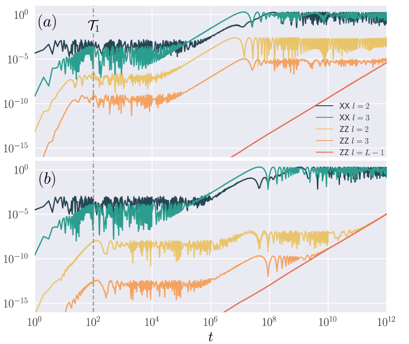
Figure 2: The dynamics of OTOCs $C_{\alpha\beta}(l,t)$ for single realizations. We set the system deep in the FTC phase (with parameters $J=h^{z}=1$, $h^{x}=0.025$ and $L=8$ spins) highlighting the OTOC in the (long) period doubling regime, $t<\mathcal{T}_{2}$. We show in panels (a) and (b) two typical dynamics for different single disorder realizations. While different OTOC directions show a qualitative similar behavior (apart from their orders of magnitude), the two instances of disorder realizations display different plateau time windows.

$\bullet\,\,\mathcal{T}_{2}<t<\mathcal{T}_{3}$: for longer times the spins decohere among each other and the FTC magnetization is slowly melted. While correlators along orthogonal directions to the $\ell$-bit protected direction (i.e., $C_{xx}(\ell,t)$) keeps its logarithmic growth till saturation, with no significant differences, the scrambling along the prefered $\tau_{i}^{z}$ direction has a rather peculiar behavior, as captured by $C_{zz}(\ell,t)$. The correlator $C_{zz}(\ell,t)$ at these late times ($t\lesssim\mathcal{T}_{2}$) has roughly saturated to a value much lower than its upper bound, with the saturated value related to the protected overlap to $\hat{\tau}_{i}^{z}$ operators. However, now due to decoherence, when the FTC starts to melt (no protected $\ell$-bit direction anymore), the correlator starts to grow again similar to thermal systems. An important observation is that, since the correlation wavefront (“lightcone”) has already passed along all the chain, the thermal growth is now independent of the distance $\ell$; therefore, the correlator $C_{zz}(\ell,t)$ have all the same growth and merge into a single one forming an envelope-like structure [72]. Precisely, in this time window the correlator $C_{zz}(\ell,t)\sim e^{-b_{\ell}\ell}+c\log(t)^{d}$, with $c,d$ independent on the distance $\ell$, where the first term stands for the saturation value achieved in the period doubling time window, and the second term arises from the onset of thermalization in the decoherence process.

$\bullet\ \,\mathcal{T}_{3}<t$: in the late time the system now is full thermal, and the OTOCs along all directions reach their maximun value.

III.3 Entanglement dynamics

We compare the scrambling of information to the dynamics of entanglement in the spins. In order to quantify the correlations we consider the entanglement entropy in an equal bipartition of the system. Specifically, given the density matrix $\hat{\rho}=|\Psi\rangle\langle\Psi|$, the total system is divided into left (A) and right (B) subsets, each with half of the total spins in the chain and corresponding reduced states $\hat{\rho}_{A(B)}=\text{Tr}_{B(A)}(|\Psi\rangle\langle\Psi|)$. The entanglement between the bipartition is defined by the von Neumann entropy of any of the reduced state,

$$S=-\frac{\text{Tr}\left[\hat{\rho}_{A}\log(\hat{\rho}_{A})\right]}{L_{A}}$$ (8)

where $L_{A}=N/2$ is size of subset $A$. In a thermal system, the entanglement entropy of an initial low entangled state typically increases linearly over time until it reaches the value associated with the system’s energy density, where the entanglement entropy obeys the thermodynamic volume law. Conversely, in a localized system, one may expect that since the information remains confined near the subsystem, the entanglement entropy should saturate at a constant value proportional to the localization length rather than the subsystem size. In fact, in AL system, the entanglement entropy saturates to a constant independent of the system size. In generic MBL systems, however, it has been observed [87, 88, 89, 79] that the entanglement entropy grows slowly, following a $\log t$ dependence in time, and saturates to a volume law at exponentially long times.

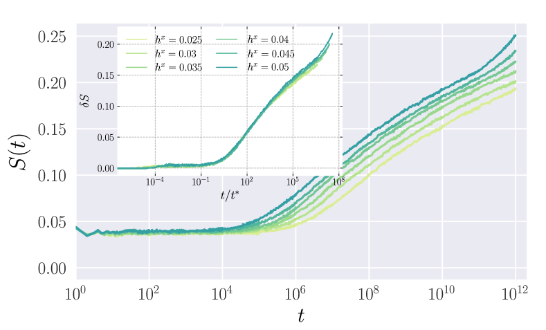
Figure 3: Dynamics of entanglement entropy $S(t)$ deep in the FTC phase ($h^{x}\approx 0$), for varying $h^{x}$ fields with a fixed system size $L=8$, and couplings $J=h^{z}=1$. The inset shows the subtracted entanglement entropy $\delta S=S_{h^{x}}(t)-S_{h^{x}=0}(t)$ with a rescaled time $t/t^{*}$.

In Fig. 3, we show the entanglement entropy calculated in deep FTC phase $h^{x}\approx 0$. In this regime, the entanglement growth obeys similar behavior as observed in a MBL system [87]. The entanglement entropy remains constant and equal to the no transverse field case, $S(h^{x}=0)$, up to a growth time $t^{*}$. The growth time is exponentially suppressed with the perturbative field $h^{x}$, specifically, as $\log t^{*}\propto(h^{x})^{-p}$ where $0<p\leq 1$. Therefore, when we renormalize the time axis with respect to growth time $t^{*}$, all curves roughly merge onto a single one (see inset Fig. 3). A similar universality is seen in different disordered system with MBL phase [87]. For time $t>t^{*}$, the entanglement shows a slow logarithmic growth, typical in the MBL. To probe the late-time entanglement dynamics, we consider larger perturbative $h^{x}$ fields. As previously discussed, the magnetization dynamics tends to a full thermalization at sufficiently late times. We find that the logarithmic growth extends till saturation time (See Fig. 4). The saturation time $t_{\text{sat}}$ grows exponentially with system-size i.e. $\log t_{\text{sat}}\sim L$, whose value obeys a volume-law.

IV Discussion

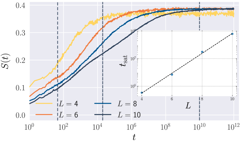
Figure 4: Late-time dynamics of entanglement entropy in the FTC phase, for varying system sizes $L$. The inset panel shows the exponential scaling of saturation time $t_{\text{sat}}$ with the number of spins. The vertical dotted lines represent the characteristic time scales $\mathcal{T}_{1,2,3}$, respectively, for $L=10$ spins. We set system parameters as $J=1=h^{z}$ and $h^{x}=0.5$.

In summary, we have investigated the dynamics of OTOCs and entanglement entropy in a disordered spin chain exhibiting Floquet time-crystal (FTC) phases. Our findings reveal distinct characteristics of information propagation within this system, governed by the presence of a quasi-protected $\ell$-bit direction. OTOCs exhibit different timescales for growth in the FTC phase, reflecting the interplay between frozen dynamics and slow logarithmic scrambling along the $\ell$-bit axis. Orthogonal to this direction, the dynamics resemble those of a conventional MBL system, with thermalization occurring at stroboscopic times. However, along the $\ell$-bit direction, a unique behavior emerges, where the system retains a stable period-doubling magnetization for exponentially long times before entering a decoherence regime characterized by logarithmic growth. At late times, the wavefront propagation of correlations completes, resulting in a uniform scrambling rate across all distances, and OTOCs converge into a single growth profile, independent of separation. Additionally, the entanglement entropy displays a persistent logarithmic increase, consistent with the slow dynamics of the system, eventually reaching a thermal volume-law saturation.

The experimental measurement of OTOCs is feasible in Floquet time crystal due to common platforms where OTOCs have been measured and where FTC have been realized. As an example, OTOCs were experimentally measured in superconducting quantum processors using a scheme that utilizes an interferometric protocol mapping correlators $C(\ell,t)$ onto the projection of an ancilla qubit [67, 66]. On the other hand, the FTC was also experimentally implemented on an array of superconducting qubits using tunable controlled-phase gates where, in fact, the same interferometric protocol was used to quantify the impact of external decoherence [38]. The observation of OTOCs in FTCs are thus promissing in such platforms; other possibilities include but are not limited to trapped atomic ions, spin-based systems, optical-lattice, neutral atoms, among others.

Future theoretical investigations could explore how scrambling manifests in other types of FTCs, such as those stabilized by Stark many-body localization [99] or quantum many-body scars [100, 101]. While this study primarily utilizes OTOCs as a probe for scrambling, alternative measures, such as Krylov complexity [102], could provide additional insights. Krylov complexity, which quantifies the delocalization of a local operator under Heisenberg evolution, has been studied in previous works [103, 104, 105] to characterize localized phases in both continuous and discrete-time systems. Extending this approach to FTCs could reveal whether and how the behavior of Krylov complexity differs from that observed in MBL systems.

Appendix A Exact OTOC evolution

In case of perfect FTC phase corresponding to parameter $h^{x}=0$ and $\phi=\pi/2$ (we will further take $T=1$ throughout), the evolution of spin-operators and therefore, OTOC can be calculated exactly. The evolution of spin-operator $\hat{\sigma}_{l}^{z}$ ($l>0$) defined as

$$\hat{\sigma}_{l}^{z}(1)=(\hat{U}_{F}\hat{U}_{K})^{\dagger}\hat{\sigma}_{l}^{z}(\hat{U}_{F}\hat{U}_{K})=\hat{U}_{K}^{\dagger}\hat{U}_{F}^{\dagger}\hat{\sigma}_{l}^{z}\hat{U}_{F}\hat{U}_{K}\,.$$ (9)

Using $[\hat{U}_{F},\hat{\sigma}_{l}^{z}]=0$ and $\hat{U}_{K}^{\dagger}\hat{\sigma}_{l}^{z}\hat{U}_{K}=-\hat{\sigma}^{z}_{l}$ — we have $\hat{\sigma}_{l}^{z}(t)=(-1)^{t}\hat{\sigma}_{l}^{z}$. Therefore, the $zz$ OTOC $F_{zz}(l,t)=\langle\hat{\sigma}^{z}_{l}(t)\hat{\sigma}_{0}^{z}\hat{\sigma}^{z}_{l}(t)\hat{\sigma}^{z}_{0}\rangle=1$ and $C_{zz}(t)=0$ showing no scrambling in $z$-direction. The evolution of spin-operators $\hat{\sigma}^{x}_{l}$ given by

$$\hat{\sigma}_{l}^{x}(1) =\hat{U}^{\dagger}_{K}\hat{U}^{\dagger}_{F}\hat{\sigma}_{l}^{x}\hat{U}_{F}\hat{U}_{K}=\sum_{ij}\exp\left[i(E(s_{j})-E(s_{i})\right]\langle\{s_{j}\}|\hat{\sigma}_{l}^{x}|\{s_{i}\}\rangle\cdot\hat{U}^{\dagger}_{K}|\{s_{j}\}\rangle\langle\{s_{i}\}|\hat{U}_{K}$$

If we represent the state $|\{s_{i}\}\rangle=|i_{0}i_{1}\ldots i_{l}\ldots\rangle$ so that

$$\langle\{s_{j}\}|\hat{\sigma}^{x}_{l}|\{s_{i}\}\rangle=\delta_{i_{0}j_{0}}\delta_{i_{1}j_{1}}\ldots\delta_{\bar{i}_{l}j_{l}}\ldots$$ (10)

where $i_{k}=\pm 1$ and $\overline{\pm 1}=\mp 1$. With this, we can write

$$\begin{split}\hat{\sigma}^{x}_{l}(1)&=\sum_{i}\exp[i(E(i_{0}i_{1}\ldots\bar{i}_{l}\ldots)-E(i_{0}i_{1}\ldots i_{l}\ldots))]|\bar{i}_{0}\bar{i}_{1}\ldots i_{l}\ldots\rangle\langle\bar{i}_{0}\bar{i}_{1}\ldots\bar{i}_{l}\ldots|\\ &=\sum_{i}e^{i\epsilon_{i}}|\bar{i}_{0}\bar{i}_{1}\ldots i_{l}\ldots\rangle\langle\bar{i}_{0}\bar{i}_{1}\ldots\bar{i}_{l}\ldots|\end{split}$$ (11)

where $\epsilon_{i}=E(i_{0}i_{1}\ldots\bar{i}_{l}\ldots)-E(i_{0}i_{1}\ldots i_{l}\ldots)=\Delta i_{l}\left(J_{l}i_{l+1}+J_{l-1}i_{l-1}+h^{z}_{l}\right)$ with $\Delta i_{l}=\bar{i}_{l}-i_{l}=\mp 2$. Following the same steps,

$$\begin{split}\hat{\sigma}^{x}_{l}(2)&=\sum_{i}e^{i\epsilon_{i}}\exp[i(E(\bar{i}_{0}\bar{i}_{1}\ldots i_{l}\ldots)-E(\bar{i}_{0}\bar{i}_{1}\ldots\bar{i}_{l}\ldots))]|i_{0}i_{1}\ldots\bar{i}_{l}\ldots\rangle\langle i_{0}i_{1}\ldots i_{l}\ldots|\\ &=\sum_{i}e^{i(\epsilon_{i}-\bar{\epsilon}_{i})}|i_{0}i_{1}\ldots\bar{i}_{l}\ldots\rangle\langle i_{0}i_{1}\ldots i_{l}\ldots|\end{split}$$ (12)

where $\bar{\epsilon_{i}}=-E(\bar{i}_{0}\bar{i}_{1}\ldots i_{l}\ldots)+E(\bar{i}_{0}\bar{i}_{1}\ldots\bar{i}_{l}\ldots)=\Delta i_{l}(J_{l}\bar{i}_{l+1}+J_{l-1}\bar{i}_{l-1}+h^{z}_{l})$. In general,

$$\hat{\sigma}^{x}_{l}(t)=\sum_{i}e^{\pm i(n\epsilon_{i}-m\bar{\epsilon}_{i})}|i_{0}i_{1}\ldots\bar{i}_{l}\ldots\rangle\langle i_{0}i_{1}\ldots i_{l}\ldots|$$ (13)

where $n=\lfloor(t+1)/2\rfloor$, $m=\lfloor t/2\rfloor$ and $\pm$ taken for even and odd time-steps, respectively. We can compute the $xx$ OTOC correlator as ($l>1$)

$$\hat{\sigma}^{x}_{l}(t)\hat{\sigma}_{0}^{x}\hat{\sigma}^{x}_{l}(t)\hat{\sigma}^{x}_{0} =\sum_{ij}e^{\pm i(n\epsilon_{i}-m\bar{\epsilon}_{i})}e^{\pm i(n\epsilon_{j}-m\bar{\epsilon}_{j})}|i_{0}i_{1}\ldots\bar{i}_{l}\ldots\rangle\langle i_{0}i_{1}\ldots i_{l}\ldots|\hat{\sigma}^{x}_{0}|j_{0}j_{1}\ldots\bar{j}_{l}\ldots\rangle\langle j_{0}j_{1}\ldots j_{l}\ldots|\hat{\sigma}^{x}_{0}$$

$$=\sum_{ij}e^{\pm i(n\epsilon_{i}-m\bar{\epsilon}_{i})}e^{\pm i(n\epsilon_{j}-m\bar{\epsilon}_{j})}|i_{0}i_{1}\ldots\bar{i}_{l}\ldots\rangle\langle i_{0}i_{1}\ldots i_{l}\ldots|\bar{j}_{0}j_{1}\ldots\bar{j}_{l}\ldots\rangle\langle\bar{j}_{0}j_{1}\ldots j_{l}\ldots|$$

$$=\sum_{j}|\bar{j}_{0}j_{1}\ldots j_{l}\ldots\rangle\langle\bar{j}_{0}j_{1}\ldots j_{l}\ldots|=I$$

it follows that $F_{xx}(t)=\langle\hat{\sigma}_{l}^{x}(t)\hat{\sigma}^{x}_{0}\hat{\sigma}^{x}_{l}(t)\hat{\sigma}^{x}_{0}\rangle=1$ and $C_{xx}(l,t)=0$. In case, when $l=1$

$$\hat{\sigma}^{x}_{1}(t)\hat{\sigma}_{0}^{x}\hat{\sigma}^{x}_{1}(t)\hat{\sigma}^{x}_{0} =\sum_{ij}e^{\pm i(n\epsilon_{i}-m\bar{\epsilon}_{i})}e^{\pm i(n\epsilon_{j}-m\bar{\epsilon}_{j})}|i_{0}\bar{i}_{1}\ldots\rangle\langle i_{0}i_{1}\ldots|\hat{\sigma}^{x}_{0}|j_{0}\bar{j}_{1}\ldots\rangle\langle j_{0}j_{1}\ldots|\hat{\sigma}^{x}_{0}$$

$$=\sum_{ij}e^{\pm i(n\epsilon_{i}-m\bar{\epsilon}_{i})}e^{\pm i(n\epsilon_{j}-m\bar{\epsilon}_{j})}|i_{0}\bar{i}_{1}\ldots\rangle\langle i_{0}i_{1}\ldots|\bar{j}_{0}\bar{j}_{1}\ldots\rangle\langle\bar{j}_{0}j_{1}\ldots|$$

$$=\sum_{j}e^{\pm iJ_{0}t\Delta j_{0}\Delta j_{1}}|j_{0}j_{1}\ldots\rangle\langle j_{0}j_{1}\ldots|$$

which is diagonal operator with diagonal elements as phases. Therefore, we can write

$$C_{xx}(1,t) =1-\mathfrak{Re}F_{xx}(1,t)=1-\langle\mathfrak{Re}(\hat{\sigma}^{x}_{1}(t)\hat{\sigma}_{0}^{x}\hat{\sigma}^{x}_{1}(t)\hat{\sigma}^{x}_{0})\rangle$$

$$=1-\sum_{j}\cos(J_{0}t\Delta j_{0}\Delta j_{1})\langle\Psi|j_{0}j_{1}\ldots\rangle\langle j_{0}j_{1}\ldots|\Psi\rangle$$

$$=1-\cos(4J_{0}t)$$ (14)

since the coupling are chosen randomly, under disorder average

$$\langle C_{xx}(1,t)\rangle=1-\frac{\cos(6Jt)\sin(2Jt)}{2t}$$ (15)

implying that $C_{xx}(1,t)\approx 1$ as $t\rightarrow\infty$. The $zx$ OTOC follows from evolution of $\hat{\sigma}^{x}_{l}$ and $\hat{\sigma}^{z}_{l}$ already computed $(l>0)$

$$\hat{\sigma}^{z}_{l}(t)\hat{\sigma}^{x}_{0}\hat{\sigma}^{z}_{l}(t)\hat{\sigma}^{x}_{0} =(-1)^{t}\hat{\sigma}^{z}_{l}\hat{\sigma}^{x}_{0}(-1)^{t}\hat{\sigma}_{l}^{z}\hat{\sigma}^{x}_{0}=\hat{\sigma}^{z}_{l}\hat{\sigma}^{x}_{0}\hat{\sigma}^{z}_{l}\hat{\sigma}^{x}_{0}=I$$

therefore, $C_{zx}(l,t)=0$ $\forall\ t$.

References

- Zaletel et al. [2023] M. P. Zaletel, M. Lukin, C. Monroe, C. Nayak, F. Wilczek, and N. Y. Yao, Rev. Mod. Phys. 95, 031001 (2023).
- Else et al. [2016] D. V. Else, B. Bauer, and C. Nayak, Phys. Rev. Lett. 117, 090402 (2016).
- von Keyserlingk and Sondhi [2016] C. W. von Keyserlingk and S. L. Sondhi, Phys. Rev. B 93, 245146 (2016).
- Khemani et al. [2016] V. Khemani, A. Lazarides, R. Moessner, and S. Sondhi, Phys. Rev. Lett. 116, 250401 (2016).
- Yao et al. [2017] N. Yao, A. Potter, I.-D. Potirniche, and A. Vishwanath, Phys. Rev. Lett. 118, 030401 (2017).
- Russomanno et al. [2017] A. Russomanno, F. Iemini, M. Dalmonte, and R. Fazio, Phys. Rev. B 95, 214307 (2017).
- Surace et al. [2019] F. M. Surace, A. Russomanno, M. Dalmonte, A. Silva, R. Fazio, and F. Iemini, Phys. Rev. B 99, 104303 (2019).
- Yang and Cai [2021] X. Yang and Z. Cai, Phys. Rev. Lett. 126, 020602 (2021).
- Morita and Kaneko [2006] H. Morita and K. Kaneko, Phys. Rev. Lett. 96, 050602 (2006).
- Ojeda Collado et al. [2021] H. P. Ojeda Collado, G. Usaj, C. A. Balseiro, D. H. Zanette, and J. Lorenzana, Phys. Rev. Res. 3, L042023 (2021).
- Nurwantoro et al. [2019] P. Nurwantoro, R. W. Bomantara, and J. Gong, Phys. Rev. B 100, 214311 (2019).
- Pizzi et al. [2021] A. Pizzi, J. Knolle, and A. Nunnenkamp, Nature Communications 12, 2341 (2021).
- Muñoz-Arias et al. [2022] M. H. Muñoz-Arias, K. Chinni, and P. M. Poggi, Phys. Rev. Res. 4, 023018 (2022).
- Giachetti et al. [2023] G. Giachetti, A. Solfanelli, L. Correale, and N. Defenu, Phys. Rev. B 108, L140102 (2023).
- Liu et al. [2023a] S. Liu, S.-X. Zhang, C.-Y. Hsieh, S. Zhang, and H. Yao, Phys. Rev. Lett. 130, 120403 (2023a).
- Lev and Lazarides [2024] Y. B. Lev and A. Lazarides, (2024), arXiv:2403.01912 [cond-mat.dis-nn] .
- Maskara et al. [2021a] N. Maskara, A. Michailidis, W. Ho, D. Bluvstein, S. Choi, M. Lukin, and M. Serbyn, Phys. Rev. Lett. 127, 090602 (2021a).
- Huang [2023] B. Huang, Phys. Rev. B 108, 104309 (2023).
- Iemini et al. [2018] F. Iemini, A. Russomanno, J. Keeling, M. Schirò, M. Dalmonte, and R. Fazio, Phys. Rev. Lett. 121, 035301 (2018).
- Souza et al. [2023] L. d. S. Souza, L. F. dos Prazeres, and F. Iemini, Phys. Rev. Lett. 130, 180401 (2023).
- Kongkhambut et al. [2022] P. Kongkhambut, J. Skulte, L. Mathey, J. G. Cosme, A. Hemmerich, and H. Keßler, Science 377, 670 (2022).
- Nakanishi and Sasamoto [2023] Y. Nakanishi and T. Sasamoto, Phys. Rev. A 107, L010201 (2023).
- Krishna et al. [2023] M. Krishna, P. Solanki, M. Hajdušek, and S. Vinjanampathy, Phys. Rev. Lett. 130, 150401 (2023).
- Li et al. [2023] X. Li, Y. Li, and J. Jin, Phys. Rev. A 107, 032219 (2023).
- Buča and Jaksch [2019] B. Buča and D. Jaksch, Phys. Rev. Lett. 123, 260401 (2019).
- Zhu et al. [2019] B. Zhu, J. Marino, N. Y. Yao, M. D. Lukin, and E. A. Demler, New Journal of Physics 21, 073028 (2019).
- Gambetta et al. [2019] F. M. Gambetta, F. Carollo, M. Marcuzzi, J. P. Garrahan, and I. Lesanovsky, Phys. Rev. Lett. 122, 015701 (2019).
- Tucker et al. [2018] K. Tucker, B. Zhu, R. J. Lewis-Swan, J. Marino, F. Jimenez, J. G. Restrepo, and A. M. Rey, New Journal of Physics 20, 123003 (2018).
- Wang et al. [2018] R. R. W. Wang, B. Xing, G. G. Carlo, and D. Poletti, Phys. Rev. E 97, 020202 (2018).
- Gong et al. [2018] Z. Gong, R. Hamazaki, and M. Ueda, Phys. Rev. Lett. 120, 040404 (2018).
- Kyprianidis et al. [2021] A. Kyprianidis et al., Science 372, 1192 (2021).
- Stasiuk and Cappellaro [2023] A. Stasiuk and P. Cappellaro, Phys. Rev. X 13, 041016 (2023).
- Beatrez et al. [2023] W. Beatrez et al., Nature Physics 19, 407 (2023).
- Mäkinen et al. [2023] J. T. Mäkinen, S. Autti, and V. B. Eltsov, Magnon Bose-Einstein condensates: from time crystals and quantum chromodynamics to vortex sensing and cosmology (2023).
- Euler et al. [2024] N. Euler, A. Braemer, L. Benn, and M. Gärttner, Phys. Rev. B 109, 224301 (2024).
- Zhang et al. [2017] J. Zhang et al., Nature 543, 217 (2017).
- Choi et al. [2017] S. Choi et al., Nature 543, 221 (2017).
- Mi et al. [2022] X. Mi et al., Nature 601, 531 (2022).
- Frey and Rachel [2022] P. Frey and S. Rachel, Science Advances 8, 10.1126/sciadv.abm7652 (2022).
- Randall et al. [2021] J. Randall et al., Science 374, 1474 (2021).
- Autti et al. [2018] S. Autti, V. B. Eltsov, and G. E. Volovik, Phys. Rev. Lett. 120, 215301 (2018).
- Autti et al. [2021] S. Autti et al., Nature Materials 20, 171 (2021).
- Iemini et al. [2024] F. Iemini, R. Fazio, and A. Sanpera, Phys. Rev. A 109, L050203 (2024).
- Montenegro et al. [2023] V. Montenegro, M. G. Genoni, A. Bayat, and M. G. A. Paris, Communications Physics 6, 1 (2023).
- Gribben et al. [2024] D. Gribben, A. Sanpera, R. Fazio, J. Marino, and F. Iemini, (2024), arXiv:2406.06273 [quant-ph] .
- Cabot et al. [2024] A. Cabot, F. Carollo, and I. Lesanovsky, Continuous sensing and parameter estimation with the boundary time crystal (2024).
- Yousefjani et al. [2024] R. Yousefjani, K. Sacha, and A. Bayat, (2024), arXiv:2405.00328 [quant-ph] .
- Moon et al. [2024] L. J. I. Moon, P. M. Schindler, R. J. Smith, E. Druga, Z.-R. Zhang, M. Bukov, and A. Ajoy, Discrete time crystal sensing (2024), arXiv:2410.05625 [quant-ph] .
- Shukla et al. [2024] R. K. Shukla, L. Chotorlishvili, S. K. Mishra, and F. Iemini, Prethermal floquet time crystals in chiral multiferroic chains and applications as quantum sensors of ac fields (2024), arXiv:2410.17530 [quant-ph] .
- Estarellas et al. [2020] M. P. Estarellas, T. Osada, V. M. Bastidas, B. Renoust, K. Sanaka, W. J. Munro, and K. Nemoto, Science Advances 6, 8892 (2020).
- Carollo et al. [2020] F. Carollo, K. Brandner, and I. Lesanovsky, Phys. Rev. Lett. 125, 240602 (2020).
- Bomantara and Gong [2018] R. W. Bomantara and J. Gong, Phys. Rev. Lett. 120, 230405 (2018).
- Lyu et al. [2020] C. Lyu, S. Choudhury, C. Lv, Y. Yan, and Q. Zhou, Phys. Rev. Res. 2, 033070 (2020).
- Bao et al. [2024] Z. Bao et al., Nature Commun. 15, 8823 (2024).
- Xu and Swingle [2024] S. Xu and B. Swingle, PRX Quantum 5, 010201 (2024).
- Lewis-Swan et al. [2019] R. J. Lewis-Swan, A. Safavi-Naini, A. M. Kaufman, and A. M. Rey, Nature Reviews Physics 1, 627 (2019).
- Deutsch [1991] J. M. Deutsch, Phys. Rev. A 43, 2046 (1991).
- Rigol et al. [2008] M. Rigol, V. Dunjko, and M. Olshanii, Nature 452, 854 (2008).
- Srednicki [1994] M. Srednicki, Phys. Rev. E 50, 888 (1994).
- Swingle [2018] B. Swingle, Nature Physics 14, 988 (2018).
- Rozenbaum et al. [2017] E. B. Rozenbaum, S. Ganeshan, and V. Galitski, Phys. Rev. Lett. 118, 086801 (2017).
- Maldacena et al. [2016] J. Maldacena, S. H. Shenker, and D. Stanford, JHEP 08, 106, arXiv:1503.01409 [hep-th] .
- Yasuhiro Sekino and L. Susskind [2008] Yasuhiro Sekino and L. Susskind, Journal of High Energy Physics 2008, 065 (2008).
- Lashkari et al. [2013] N. Lashkari, D. Stanford, M. Hastings, T. Osborne, and P. Hayden, Journal of High Energy Physics 2013, 22 (2013).
- Shenker and Stanford [2014] S. H. Shenker and D. Stanford, JHEP 03, 067, arXiv:1306.0622 [hep-th] .
- Swingle et al. [2016] B. Swingle, G. Bentsen, M. Schleier-Smith, and P. Hayden, Phys. Rev. A 94, 040302 (2016).
- Mi et al. [2021] X. Mi et al., Science 374, 1479 (2021).
- Zhao et al. [2022] S. K. Zhao et al., Phys. Rev. Lett. 129, 160602 (2022).
- Gärttner et al. [2017] M. Gärttner, J. G. Bohnet, A. Safavi-Naini, M. L. Wall, J. J. Bollinger, and A. M. Rey, Nature Physics 13, 781 (2017).
- Braumüller et al. [2022] J. Braumüller et al., Nature Physics 18, 172 (2022).
- Landsman et al. [2019] K. A. Landsman et al., Nature 567, 61 (2019).
- Xu and Swingle [2020] S. Xu and B. Swingle, Nature Physics 16, 199 (2020).
- Luitz and Bar Lev [2017] D. J. Luitz and Y. Bar Lev, Phys. Rev. B 96, 020406 (2017).
- Bohrdt et al. [2017] A. Bohrdt, C. B. Mendl, M. Endres, and M. Knap, New Journal of Physics 19, 063001 (2017).
- Lin and Motrunich [2018] C.-J. Lin and O. I. Motrunich, Phys. Rev. B 97, 144304 (2018).
- Burrell and Osborne [2007] C. K. Burrell and T. J. Osborne, Phys. Rev. Lett. 99, 167201 (2007).
- Swingle and Chowdhury [2017] B. Swingle and D. Chowdhury, Phys. Rev. B 95, 060201 (2017).
- Pal and Huse [2010] A. Pal and D. A. Huse, Phys. Rev. B 82, 174411 (2010).
- Abanin et al. [2019] D. A. Abanin, E. Altman, I. Bloch, and M. Serbyn, Rev. Mod. Phys. 91, 021001 (2019).
- Nandkishore and Huse [2015] R. Nandkishore and D. A. Huse, Annual Review of Condensed Matter Physics 6, 15 (2015).
- Vosk et al. [2015] R. Vosk, D. A. Huse, and E. Altman, Phys. Rev. X 5, 031032 (2015).
- Altman [2018] E. Altman, Nature Physics 14, 979 (2018).
- Chen et al. [2017] X. Chen, T. Zhou, D. A. Huse, and E. Fradkin, Annalen der Physik 529, 1600332 (2017).
- Slagle et al. [2017] K. Slagle, Z. Bi, Y.-Z. You, and C. Xu, Phys. Rev. B 95, 165136 (2017).
- He and Lu [2017] R.-Q. He and Z.-Y. Lu, Phys. Rev. B 95, 054201 (2017).
- Sahu et al. [2019] S. Sahu, S. Xu, and B. Swingle, Phys. Rev. Lett. 123, 165902 (2019).
- Bardarson et al. [2012] J. H. Bardarson, F. Pollmann, and J. E. Moore, Phys. Rev. Lett. 109, 017202 (2012).
- Dumitrescu et al. [2017] P. T. Dumitrescu, R. Vasseur, and A. C. Potter, Phys. Rev. Lett. 119, 110604 (2017).
- Khemani et al. [2017] V. Khemani, S. P. Lim, D. N. Sheng, and D. A. Huse, Phys. Rev. X 7, 021013 (2017).
- Sierant et al. [2023] P. Sierant, M. Lewenstein, A. Scardicchio, and J. Zakrzewski, Phys. Rev. B 107, 115132 (2023).
- Xu et al. [2021] H. Xu, J. Zhang, J. Han, Z. Li, G. Xue, W. Liu, Y. Jin, and H. Yu, (2021), arXiv:2108.00942 [quant-ph] .
- Lee et al. [2019] J. Lee, D. Kim, and D.-H. Kim, Phys. Rev. B 99, 184202 (2019).
- Fan et al. [2017] R. Fan, P. Zhang, H. Shen, and H. Zhai, Science Bulletin 62, 707 (2017).
- Huse et al. [2014] D. A. Huse, R. Nandkishore, and V. Oganesyan, Phys. Rev. B 90, 174202 (2014).
- Ros et al. [2015] V. Ros, M. Müller, and A. Scardicchio, Nuclear Physics B 891, 420 (2015).
- Tang et al. [2015] B. Tang, D. Iyer, and M. Rigol, Phys. Rev. B 91, 161109 (2015).
- Serbyn et al. [2013] M. Serbyn, Z. Papić, and D. A. Abanin, Phys. Rev. Lett. 111, 127201 (2013).
- Imbrie [2016] J. Z. Imbrie, Journal of Statistical Physics 163, 998 (2016).
- Liu et al. [2023b] S. Liu, S.-X. Zhang, C.-Y. Hsieh, S. Zhang, and H. Yao, Phys. Rev. Lett. 130, 120403 (2023b).
- Bull et al. [2022] K. Bull, A. Hallam, Z. Papić, and I. Martin, Phys. Rev. Lett. 129, 140602 (2022).
- Maskara et al. [2021b] N. Maskara, A. A. Michailidis, W. W. Ho, D. Bluvstein, S. Choi, M. D. Lukin, and M. Serbyn, Phys. Rev. Lett. 127, 090602 (2021b).
- Parker et al. [2019] D. E. Parker, X. Cao, A. Avdoshkin, T. Scaffidi, and E. Altman, Phys. Rev. X 9, 041017 (2019).
- Sahu et al. [2024] H. Sahu, A. Bhattacharya, and P. P. Nath, (2024), arXiv:2409.03656 [quant-ph] .
- Trigueros and Lin [2022] F. B. Trigueros and C.-J. Lin, SciPost Phys. 13, 037 (2022).
- Sahu [2024] H. Sahu, Phys. Rev. A 110, 052405 (2024).