Sampling and Integration of Logconcave Functions by
Algorithmic Diffusion

Abstract

We study the complexity of sampling, rounding, and integrating arbitrary logconcave functions. Our new approach provides the first complexity improvements in nearly two decades for general logconcave functions for all three problems, and matches the best-known complexities for the special case of uniform distributions on convex bodies. For the sampling problem, our output guarantees are significantly stronger than previously known, and lead to a streamlined analysis of statistical estimation based on dependent random samples.

1 Introduction

Sampling and integration of logconcave functions are fundamental problems with numerous applications and important special cases such as uniform distributions over convex bodies and strongly logconcave densities. The study of these problems has led to many useful techniques. Both mathematically and algorithmically, general logconcave functions typically provide the “right” general abstraction. For example, many classical inequalities for convex bodies have natural extensions to logconcave functions (e.g., Grünbaum’s theorem, Brunn-Minkowski and Prékopa-Leindler, isotropic constant, etc.). The KLS hyperplane conjecture, first motivated by the analysis of the $\mathsf{Ball\ Walk}$ for sampling convex bodies, is in the setting of general logconcave densities. The current fastest algorithm for estimating the volume of a convex body crucially uses sampling from a sequence of logconcave densities, which is provably more efficient than using a sequence of uniform distributions. Sampling logconcave densities has many other applications as well, such as portfolio optimization, simulated annealing, Bayesian inference, differential privacy etc.

Sampling in high dimension is done by randomized algorithms based on Markov chains. These chains are set up to have a desired stationary distribution, which is relatively easy to ensure. For example, to sample uniformly, it suffices that the Markov chain is symmetric. Generally, to sample proportional to a desired function, it suffices to ensure the “detailed balance” condition. The main challenge is showing rapid mixing of the Markov chain, i.e., the convergence rate to the stationary distribution is bounded by a (small) polynomial in the dimension and other relevant parameters.

The traditional analysis of Markov chains for sampling high-dimensional distributions proceeds by analyzing the conductance of the Markov chain, the minimum conditional escape probability over all subsets of the state space of measure at most half. Bounding this is done by relating probabilistic (one-step distribution) distance to geometric distance, and then using a purely isoperimetric inequality for subsets of the support. Indeed, this approach led to several interesting questions and useful techniques, in particular the development of isoperimetric inequalities and the discovery of (nearly) tight bounds in many settings. To describe background and known results, let us first define the sampling problem (readers familiar with the problem can skip to §1.1).

Model and problems.

We assume access to an integrable logconcave function $\exp(-V(x))$ in $\mathbb{R}^{n}$, via an evaluation oracle for a convex function $V:\mathbb{R}^{n}\to\mathbb{R}\cup\{\infty\}$. We also assume that there exists a point $x_{0}$ and parameters $r,R$ such that for the distribution $\pi$ with density $\mathrm{d}\pi\propto\exp(-V)\,\mathrm{d}x$, a ball of radius $r$ centered at $x_{0}$ is contained in the level set of $\pi$ of measure $1/8$ and $\mathbb{E}_{\pi}[\lVert X-x_{0}\rVert^{2}]\leq R^{2}$. We refer to this as a well-defined function oracle, denoted by $\mathsf{Eval}_{\mathcal{P}}(V)$ where $\mathcal{P}$ indicates access to the actual values of parameters in $\mathcal{P}$ (e.g., $\mathsf{Eval}_{x_{0},R}(V)$ presents both $x_{0}$ and $R$, while $\mathsf{Eval}(V)$ does not provide any parameters).

Given this oracle, in this paper we consider three central problems: (1) sample from the distribution $\pi$, (2) find an affine transformation that places $\pi$ in near-isotropic position, and (3) estimate the integral $\int e^{-V(x)}\,\mathrm{d}x$ (i.e., the normalization constant of $\pi$). We measure the complexity in terms of the number of oracle calls and the total number of arithmetic operations.

Complexity of logconcave sampling.

Sampling general logconcave functions, as an algorithmic problem, was first studied by Applegate and Kannan [AK91], who established an algorithm with complexity polynomial in the dimension assuming Lipschitzness of the function over its support. They did this by creating a sufficiently fine grid (so that the function changed by at most a small constant within each grid cell) and used a discrete “grid walk”. They sampled a grid point and used rejection sampling to output a point from the cube associated with the grid point. The output distribution is guaranteed to be within desired total variation ($\mathsf{TV}$) distance from the target distribution. Following many developments, Lovász and Vempala improved the bound to scale as $n^{2}R^{2}/r^{2}$ [LV07, LV06a]. More specifically, [LV07, Theorem 2.2, 2.3] analyzed the $\mathsf{Ball\ Walk}$ and $\mathsf{Hit\text{-}and\text{-}Run}$ and proved a bound of

$$\frac{M^{4}}{\varepsilon^{4}}\frac{n^{2}R^{2}}{r^{2}}\log\frac{M}{\varepsilon}$$

steps/queries to reach a distribution within $\varepsilon$ $\mathsf{TV}$-distance of the target starting from an $M$-warm distribution. [LV06a, Theorem 1.1] showed that $\mathsf{Hit\text{-}and\text{-}Run}$ achieves the same guarantee in

$$\frac{n^{2}R^{2}}{r^{2}}\log^{\mathcal{O}(1)}\frac{nMR}{\varepsilon r}$$

steps. We note that in all previous work on general logconcave sampling the output guarantees are in $\mathsf{TV}$-distance. It is often desirable to have stronger guarantees such as the $\mathsf{KL}$ or Rényi divergences.

Classical sampling algorithms.

For target density proportional to $e^{-V}$, the $\mathsf{Ball\ Walk}$ with parameter $\delta$ proceeds as follows: at a point $x$ with $e^{-V(x)}>0$, sample a uniform random point $y$ in the ball of radius $\delta$ centered at $x$; go to $y$ with probability $\min(1,\frac{e^{-V(y)}}{e^{-V(x)}})$, staying at $x$ with the remaining probability. $\mathsf{Hit\text{-}and\text{-}Run}$ does not need a parameter: at current point $x$, pick a uniform random line $\ell$ through $x$, and go to a random point $y$ along $\ell$ with probability proportional to $e^{-V(y)}$ (marginal along $\ell$). For technical reasons, both of these walks (and almost all other walks) need to be lazy, i.e., they do nothing with probability $1/2$, and do the above step with probability $1/2$.

Sampling and isoperimetry.

The complexity of sampling is intuitively tied closely to the isoperimetry of the target distribution. If the target has poor isoperimetry (roughly, a small measure surface can partition the support into two large measure subsets), then any “local” Markov chain will have difficulty moving from one large subset to its complement. There are two alternative views of isoperimetry — functional and geometric. We recap the definitions of isoperimetric constants.

Definition 1.1.

We say that a probability measure $\pi$ on $\mathbb{R}^{n}$ satisfies a Poincaré inequality (PI) with parameter $C_{\mathsf{PI}}(\pi)$ if for all smooth functions $f:\mathbb{R}^{n}\to\mathbb{R}$,

$$\operatorname{var}_{\pi}f\leq C_{\mathsf{PI}}(\pi)\,\mathbb{E}_{\pi}[\lVert\nabla f\rVert^{2}]\,, \mathsf{PI}$$ ()

where $\operatorname{var}_{\pi}f=\mathbb{E}_{\pi}[\lvert f-\mathbb{E}_{\pi}f\rvert^{2}]$.

The Poincaré inequality is implied by the generally stronger log-Sobolev inequality.

Definition 1.2.

We say that a probability measure $\pi$ on $\mathbb{R}^{n}$ satisfies a log-Sobolev inequality (LSI) with parameter $C_{\mathsf{LSI}}(\pi)$ if for all smooth functions $f:\mathbb{R}^{n}\to\mathbb{R}$,

$$\operatorname{Ent}_{\pi}(f^{2})\leq 2C_{\mathsf{LSI}}(\pi)\,\mathbb{E}_{\pi}[\lVert\nabla f\rVert^{2}]\,, \mathsf{LSI}$$ ()

where $\operatorname{Ent}_{\pi}(f^{2}):=\mathbb{E}_{\pi}[f^{2}\log f^{2}]-\mathbb{E}_{\pi}[f^{2}]\log\mathbb{E}_{\pi}[f^{2}]$.

For the geometric view, we define $\pi(\partial S):=\liminf_{\varepsilon\downarrow 0}\frac{\pi(S_{\varepsilon})-\pi(S)}{\varepsilon}$, where $S_{\varepsilon}:=\{x:d(x,S)\leq\varepsilon\}$.

Definition 1.3.

The Cheeger constant $C_{\mathsf{Ch}}(\pi)$ of a probability measure $\pi$ on $\mathbb{R}^{n}$ is defined as

$$C_{\mathsf{Ch}}(\pi)=\inf_{S\subset\mathbb{R}^{n},\pi(S)\leq\frac{1}{2}}\frac{\pi(\partial S)}{\pi(S)}\,.$$

Definition 1.4.

The log-Cheeger constant $C_{\mathsf{logCh}}(\pi)$ of a probability measure $\pi$ on $\mathbb{R}^{n}$ is defined as

$$C_{\mathsf{logCh}}(\pi)=\inf_{S\subset\mathbb{R}^{n},\pi(S)\leq\frac{1}{2}}\frac{\pi(\partial S)}{\pi(S)\sqrt{\log(1/\pi(S))}}\,.$$

It is known that for logconcave measures, $C_{\mathsf{PI}}(\pi)=\Theta(C_{\mathsf{Ch}}^{-2}(\pi))$ [Mil09] and $C_{\mathsf{LSI}}(\pi)=\Theta(C_{\mathsf{logCh}}^{-2}(\pi))$ [Led94]. Bounding these constants has been a major research topic for decades. In recent years, following many improvements, it has been shown that for isotropic logconcave measures, $C_{\mathsf{PI}}(\pi)\lesssim\log n$ [Kla23] and for isotropic logconcave ones with support of diameter $D$, we have $C_{\mathsf{LSI}}(\pi)\lesssim D$ [LV24]. The former is conjectured to be $\mathcal{O}(1)$ (the KLS conjecture), and the latter is the best possible.

The significance of these constants for algorithmic sampling became clear with the analysis of the $\mathsf{Ball\ Walk}$, where the bound on its convergence from a warm start to a logconcave distribution depends directly on $C_{\mathsf{Ch}}^{-2}(\pi)$ [KLS97] (this was the original motivation for the KLS conjecture) — the mixing time of the $\mathsf{Ball\ Walk}$ starting from an $M$-warm distribution to reach $\varepsilon$ $\mathsf{TV}$-distance is bounded by $\mathcal{O}(n^{2}C_{\mathsf{Ch}}^{-2}\operatorname{poly}\frac{M}{\varepsilon})$. For the special case of uniformly sampling convex bodies, using the notion of a $\mathsf{Speedy\ Walk}$, this can be improved to $\mathcal{O}(Mn^{2}C_{\mathsf{Ch}}^{-2}\log\frac{M}{\varepsilon})$, but using it in the analysis entails handling several technical difficulties. In principle, this should be extendable to general logconcave functions, albeit with formidable technical complications. We take a different approach.

Sampling, isoperimetry, and diffusion.

The connection of isoperimetric constants to the convergence of continuous-time diffusion is a classical subject. The Langevin diffusion is a canonical stochastic differential equation (SDE) given by

$$\mathrm{d}X_{t}=-\nabla V(X_{t})\,\mathrm{d}t+\sqrt{2}\,\mathrm{d}B_{t}\quad X_{0}\sim\nu_{0}\,,$$

where $B_{t}$ is the standard Brownian process, and $V$ is a smooth function. Then, under mild conditions, the law $\nu_{t}$ of $X_{t}$ converges to the distribution with density $\nu$ proportional to $e^{-V}$ in the limit. Moreover, it can be shown that

$$\chi^{2}(\nu_{t}\mathbin{\|}\nu)\leq\exp\bigl{(}-\frac{2t}{C_{\mathsf{PI}}(\nu)}\bigr{)}\,\chi^{2}(\nu_{0}\mathbin{\|}\nu)\,,\quad\text{and}\quad\mathsf{KL}(\nu_{t}\mathbin{\|}\nu)\leq\exp\bigl{(}-\frac{2t}{C_{\mathsf{LSI}}(\nu)}\bigr{)}\,\mathsf{KL}(\nu_{0}\mathbin{\|}\nu)\,.$$

A natural idea for a sampling algorithm is to discretize the diffusion equation. This discretized algorithm was shown to converge in $\text{poly}(n,\beta,C_{\mathsf{PI}}(\nu))$ and $\text{poly}(n,\beta,C_{\mathsf{LSI}}(\nu))$ iterations under ($\mathsf{PI}$) [CEL⁺22] and ($\mathsf{LSI}$) [VW19] respectively, assuming $\beta$-Lipschitzness of $\nabla V$. Can this approach be extended to sampling general logconcave densities without the gradient Lipschitzness?

Algorithmic diffusion.

By algorithmic diffusion, we mean the general idea of discretizing a diffusion process and proving guarantees on the discretization error and query complexity. Recently, [KVZ24] showed that such an algorithm (called $\mathsf{\mathsf{In\text{-}and\text{-}Out}}$ there), which can be viewed as a $\mathsf{Proximal\ Sampler}$, works for sampling from the uniform distribution over a convex body and recovers state-of-the-art complexity guarantees with substantially improved output guarantees (Rényi-divergences). The guarantee was extended to the Rényi-infinity (or pointwise) distance as well [KZ25]. A nice aspect of the analysis is that it shows convergence directly in terms of isoperimetric constants of target distributions. As a result, it provides a unifying point of view for analysis without requiring the use of technically sophisticated tools such as the $\mathsf{Speedy\ Walk}$ and $s$-conductance [LS93, KLS97, LV07]. We discuss the approach in more detail presently.

This brings us to the main motivation of the current paper: Can we use algorithmic diffusion to obtain faster algorithms with stronger guarantees for sampling, rounding, and integrating general logconcave functions?

1.1 Results

In this paper, we propose new approaches for general logconcave sampling, rounding and integration, leading to the first improvements in the complexity of these problems in nearly two decades [LV06a]. Our methods crucially rely on a reduction from general logconcave sampling to exponential sampling in one higher dimension. With this reduction in hand, we develop a new framework for sampling and improve the complexity of four fundamental problems: (1) logconcave sampling from an $\mathcal{O}(1)$-warm start, (2) warm-start generation, (3) isotropic rounding and (4) integration. For each problem, our improved complexity for general logconcave distributions matches the current best complexity for the uniform distribution over a convex body, a setting that has received much attention for more than three decades [DFK91, LS90, Lov91, LS93, KLS97, LV06b, CV18, KVZ24, KZ25]. We now present our main results, followed by a detailed discussion of the challenges and techniques in §1.2, and notations and preliminaries in §1.3.

Result 1: Logconcave sampling from a warm start.

When a logconcave distribution $\pi^{X}\propto e^{-V}$ is presented with the evaluation oracle for $V$, we instead consider the “lifted” distribution

$$\pi(x,t)\propto\exp(-nt)\cdot\mathds{1}[(x,t):V(x)\leq nt]$$

in the augmented $(x,t)$-space, the $X$-marginal of which is exactly $\pi^{X}$ (see Proposition 2.3). We quantify in §2 how this affects parameters pertinent to sampling (e.g., isoperimetric constants).

Input: initial pt. $z_{0}\sim\pi_{0}\in\mathcal{P}(\mathbb{R}^{n+1})$, $\mathcal{K}=\{(x,t):V(x)\leq nt\}$, $k\in\mathbb{N}$, threshold $N$, variance $h$.

Output: $z_{k+1}=(x_{k+1},t_{k+1})$.

1:  for $i=0,\dotsc,k$ do

2:     Sample $y_{i+1}\sim\mathcal{N}(z_{i},hI_{n+1})$.

3:     Sample $z_{i+1}\sim\mathcal{N}(y_{i+1}-hne_{n+1},hI_{n+1})|_{\mathcal{K}}$.

4:     $\quad(\uparrow)$ Repeat $z_{i+1}\sim\mathcal{N}(y_{i+1}-hne_{n+1},hI_{n+1})$ until $z_{i+1}\in\mathcal{K}$. If $\#$attempts${}_{i}\,\geq N$, declare Failure.

5:  end for

Algorithm 1 $\mathsf{Proximal\ Sampler}$ $\mathsf{PS}_{\textup{exp}}$

To sample from the exponential target $\pi$ using a given $\mathcal{R}_{\infty}$ warm-start, we use the $\mathsf{Proximal\ Sampler}$ (see Figure 1.1) with an evaluation oracle that returns $nt$ conditioned on $V(x)\leq nt$. One iteration of the sampler is reversible with respect to the stationary distribution $\pi$, while it can be interpreted as a composition of two complimentary diffusion processes. Discarding the $T$-component of a sample, we are left with the $X$-component with law close to our desired target $\pi^{X}$. In this regard, our sampler is a natural generalization of $\mathsf{\mathsf{In\text{-}and\text{-}Out}}$ [KVZ24], the $\mathsf{Proximal\ Sampler}$ for uniform sampling. Concretely, we establish mixing guarantees and query complexities of our sampler for the target logconcave distribution $\pi^{X}$ in terms of its Poincaré constant (which in general satisfies $\lVert\operatorname{Cov}\pi^{X}\rVert\leq C_{\mathsf{PI}}(\pi^{X})\lesssim\lVert\operatorname{Cov}\pi^{X}\rVert\log n$ [Kla23]).

Theorem 1.5.

For any logconcave distribution $\pi^{X}$ specified by a well-defined function oracle $\mathsf{Eval}(V)$, for any given $\eta,\varepsilon\in(0,1)$, $q\geq 2$, and $\pi_{0}^{X}$ with $\mathcal{R}_{\infty}(\pi_{0}^{X}\mathbin{\|}\pi^{X})=\log M$, we can use the $\mathsf{Proximal\ Sampler}$ $\mathsf{PS}_{\textup{exp}}$ (Algorithm 1) with suitable choices of parameters, so that with probability at least $1-\eta$, we obtain a sample $X$ such that $\mathcal{R}_{q}(\operatorname{law}X\mathbin{\|}\pi^{X})\leq\varepsilon$, using $\widetilde{\mathcal{O}}(qMn^{2}\,(\lVert\operatorname{Cov}\pi^{X}\rVert\vee 1)\operatorname{polylog}\frac{1}{\eta\varepsilon})$ evaluation queries in expectation.

See §2.2.1 for a more detailed description of the heat flow perspective and its benefits for sampling. Our specific setting of parameters can be found in Theorem 2.15. In comparison with the previous best complexity of $\widetilde{\mathcal{O}}(n^{2}\operatorname{tr}(\operatorname{Cov}\pi^{X})\operatorname{polylog}\frac{M}{\varepsilon})$, which is for $\mathsf{TV}$-distance, the $\mathsf{Proximal\ Sampler}$ $\mathsf{PS}_{\textup{exp}}$ achieves a provably better rate (since $\lVert\operatorname{Cov}\pi^{X}\rVert\leq\operatorname{tr}(\operatorname{Cov}\pi^{X})$) from an $\mathcal{O}(1)$-warm start, and moreover does so in general $\mathcal{R}_{q}$-divergences. This mixing rate matches the previously known best rate for the uniform sampling by the $\mathsf{Ball\ Walk}$ [KLS97] as well as $\mathsf{\mathsf{In\text{-}and\text{-}Out}}$ [KVZ24].

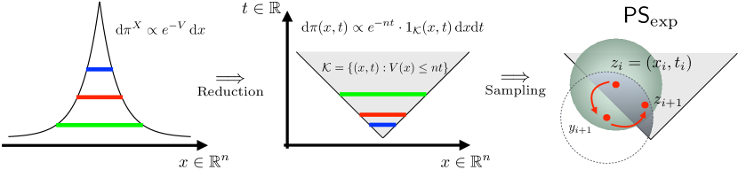
Figure 1.1: Reduction to an exponential distribution and sampling via the $\mathsf{Proximal\ Sampler}$ $\mathsf{PS}_{\textup{exp}}$.

Result 2: Warm-start generation (sampling without a warm start).

The $\mathsf{Proximal\ Sampler}$ $\mathsf{PS}_{\textup{exp}}$ assumes access to a warm start in $\mathcal{R}_{\infty}$, and generating such a good warm-start is an important and challenging algorithmic problem in its own right. In §3, we propose $\mathsf{Tilted\ Gaussian\ Cooling}$ which generates an $\mathcal{O}(1)$-warm start in the $\mathcal{R}_{\infty}$-divergence for any target logconcave distribution. This algorithm generalizes $\mathsf{Gaussian\ Cooling}$ [CV18], the known method for generating a warm-start for the uniform distribution over a convex body. The high-level idea is to follow a sequence $\{\mu_{i}\}_{i\in[m]}$ of distributions, where $\mu_{1}$ is easy to sample from, $\mu_{i}$ and $\mu_{i+1}$ are close in some probability divergences, and $\mu_{m}$ is the desired target.

Our algorithm first reduces the original target to the exponential distribution and then follows annealing distributions of the form

$$\mu_{\sigma^{2},\rho}(x,t)\propto\exp\bigl{(}-\frac{1}{2\sigma^{2}}\,\lVert x\rVert^{2}-\rho t\bigr{)}\cdot\mathds{1}[\{V(x)\leq nt\}\cap\{\lVert x\rVert=\mathcal{O}(R),\lvert t\rvert=\mathcal{O}(1)\}]\,,$$

with a carefully chosen schedule for updating the parameters $\sigma^{2}$ and $\rho$. Roughly speaking, we update the $X$-marginal through $\mathsf{Gaussian\ Cooling}$ and the $T$-marginal using an exponential tilt. In order to move across the annealing distributions, $\mathsf{Tilted\ Gaussian\ Cooling}$ requires an efficient sampler for the intermediate annealing distributions, ideally with guarantees in the $\mathcal{R}_{\infty}$-divergence in order to relay $\mathcal{R}_{\infty}$-warmness guarantees along the annealing scheme. We use the $\mathsf{Proximal\ Sampler}$ for these intermediate distributions with a $\mathcal{R}_{\infty}$-divergence guarantee, namely the $\mathsf{Proximal\ Sampler}$ $\mathsf{PS}_{\textup{ann}}$ (Algorithm 3) in §3.2. In our computational model, this sampler started at a previous annealing distribution returns a sample with law $\mu$ satisfying $\mathcal{R}_{\infty}(\mu\mathbin{\|}\mu_{\sigma^{2},\rho})\leq\varepsilon$, using $\widetilde{\mathcal{O}}(n^{2}\sigma^{2}\operatorname{polylog}\nicefrac{{R}}{{\eta\varepsilon}})$ evaluation queries in expectation (see Theorem 3.11).

By sampling these annealing distributions through $\mathsf{PS}_{\textup{ann}}$, $\mathsf{Tilted\ Gaussian\ Cooling}$ obtains an $\mathcal{O}(1)$-warm start for $\pi$ (and hence for the desired target $\pi^{X}$); then runs the $\mathsf{Proximal\ Sampler}$ $\mathsf{PS}_{\textup{exp}}$ one final time to obtain a sample with $\mathcal{R}_{\infty}$-guarantees (this is a very strong notion of probability divergence that recovers all commonly used distances such as $\mathsf{TV},\mathsf{KL},\chi^{2},$ or $\mathcal{R}_{q}$).

Theorem 1.6.

For any logconcave distributions $\pi^{X}$ specified by $\mathsf{Eval}_{x_{0},R}(V)$, for any given $\eta,\varepsilon\in(0,1)$, $\mathsf{Tilted\ Gaussian\ Cooling}$ (Algorithm 2) with probability at least $1-\eta$, returns a sample with law $\nu$ such that $\mathcal{R}_{\infty}(\nu\mathbin{\|}\pi^{X})\leq\varepsilon$, using $\widetilde{\mathcal{O}}(n^{2}(R^{2}\vee n)\operatorname{polylog}\nicefrac{{1}}{{\eta\varepsilon}})$ evaluation queries in expectation. Hence, if $\pi^{X}$ is well-rounded (i.e., $R^{2}\lesssim n$), then $\widetilde{\mathcal{O}}(n^{3}\operatorname{polylog}\nicefrac{{1}}{{\eta\varepsilon}})$ queries suffice.

This improves the prior best complexity of $\widetilde{\mathcal{O}}(n^{3}R^{2}\operatorname{polylog}\frac{1}{\varepsilon})$ for general logconcave sampling (in $\mathsf{TV}$-distance) from scratch by [LV06a, Collorary 1.2], and provides a much stronger $\mathcal{R}_{\infty}$-guarantee. Moreover, this complexity matches the best-known complexity for uniform sampling with the $\mathsf{TV}$-guarantee by [CV18] and with the $\mathcal{R}_{\infty}$-guarantee by [KZ25].

Result 3: Isotropic rounding of logconcave distributions.

The above results on the complexity of logconcave sampling still have dependence on the second moment $R^{2}$, so those are not fully polynomial in the problem parameters. In §4, we address this issue by initially running an algorithm for isotropic rounding which makes the covariance matrix of a given logconcave distribution near-isotropic (i.e., $\operatorname{Cov}\pi^{X}\approx I_{n}$). After this rounding, $R^{2}=\mathcal{O}(n)$, and thus the guarantee above turns into $n^{3}$ at the cost of a multiplicative factor of $\operatorname{polylog}R$ in the complexity. Isotropic rounding is also a useful tool for many other high-dimensional algorithms.

At a high level, just as in the warm-start generation, our algorithm follows a sequence $\{\mu_{i}\}$ of distributions while updating an affine map $F:\mathbb{R}^{n}\to\mathbb{R}^{n}$ along the way. An important subroutine is to convert a well-rounded distribution (i.e., with $\operatorname{tr}(\operatorname{Cov})=\mathcal{O}(n)$) to one that is near-isotropic (i.e., with $\operatorname{Cov}\approx I_{n}$). To this end, we generalize the approach taken in [JLLV21] for the uniform distribution — repeatedly [draw a few samples $\to$ compute a crude estimate of the covariance $\to$ identify skewed directions from the estimation and upscale them]. In doing so, we rely crucially on our sampler’s mixing rate in terms of $\lVert\operatorname{Cov}\pi^{X}\rVert$ (instead of $\operatorname{tr}(\operatorname{Cov}\pi^{X})$) in Result 1 and its improved complexity for warm-start generation in Result 2.

Theorem 1.7.

For any logconcave distribution $\pi^{X}$ specified by $\mathsf{Eval}_{x_{0},R}(V)$, there exists a randomized algorithm with query complexity of $\widetilde{\mathcal{O}}(n^{3.5}\operatorname{polylog}R)$ that finds an affine map $F$ such that the pushforward of $\pi^{X}$ via $F$ is $1.01$-isotropic with probability at least $1-\mathcal{O}(n^{-1/2})$.

Our complexity improves upon the previous best complexity of $\widetilde{\mathcal{O}}(n^{4}\operatorname{polylog}R)$ for general logconcave distributions [LV06a, Theorem 6.1]. Moreover, our rate matches that of isotropic rounding for the uniform distribution [JLLV21, JLLV24].

Result 4: Integration of logconcave functions.

Finally, we examine the complexity of integrating a logconcave function, a classical application of logconcave sampling. To this end, we extend an annealing approach in [CV18] to general logconcave integration in §5. Similar to $\mathsf{Tilted\ Gaussian\ Cooling}$, we follow a sequence $\{f_{i}\}_{i\in[m]}$ of logconcave functions, where $f_{1}$ is easy to integrate, $\mu_{i}\propto f_{i}$ is an $\mathcal{O}(1)$-warm start for $\mu_{i+1}\propto f_{i+1}$, the variance of $f_{i+1}/f_{i}$ with respect to $\mu_{i}$ is small enough (e.g., $\chi^{2}(\mu_{i+1}\mathbin{\|}\mu_{i})=\mathcal{O}(m^{-1})$), and $f_{m}$ is the target logconcave function.

Theorem 1.8.

For any $\varepsilon>0$ and an integrable well-rounded logconcave function $f=e^{-V}:\mathbb{R}^{n}\rightarrow\mathbb{R}$ presented by $\mathsf{Eval}_{x_{0},R}(V)$, there exists an algorithm that with probability at least $3/4$, returns a $(1+\varepsilon)$-multiplicative approximation to the integral of $f$ using $\widetilde{\mathcal{O}}(n^{3}/\varepsilon^{2})$ queries. For an arbitrary logconcave $f$ given by a well-defined function oracle, the complexity is bounded by $\widetilde{\mathcal{O}}(n^{3.5}\operatorname{polylog}R+n^{3}/\varepsilon^{2})$.

This result improves the previous best complexity $\widetilde{\mathcal{O}}(n^{4}/\varepsilon^{2})$ of integrating logconcave functions [LV06a, Theorem 1.3]. Again, our improved complexity matches that for the uniform distribution (i.e., volume computation) [CV18, JLLV21, JLLV24]. We note that due to the strong guarantees of the new sampler, we can streamline the analysis of errors and dependence among samples used to estimate $f_{i+1}/f_{i}$, simplifying and strengthening earlier analyses [KLS97, LV06c, CV18].

1.2 Techniques and background

In proving our results — faster algorithms for the basic problems of sampling (with and without a warm start), rounding and integration — we do not take the most direct route. Instead we develop several techniques that appear to be interesting and we imagine will be useful in other contexts as well. These include the reversible heat-flow perspective for the design of polynomial-time algorithms providing a direct connection to isoperimetric constants, sampling guarantees in the strong notion of $\mathcal{R}_{\infty}$-distance (which has other motivations such as differential privacy), relevant geometry of logconcave functions, and a streamlined analysis of estimation errors of dependent samples.

1.2.1 Going beyond the uniform distribution

The uniform distribution over a convex body is a special case of a logconcave distribution. The best-known polynomial complexity for uniform sampling is achieved by addressing three subproblems: (1) sampling from a warm start, (2) generating a warm start and (3) performing isotropic rounding. Extending the best-known guarantees and algorithms for each of these problems to general logconcave densities is the primary challenged addressed in this paper. In our proofs, we use general properties of logconcave functions and avoid any structural assumptions on the target density.

The first challenge is to establish a logconcave sampler with a mixing rate matching that of the best uniform samplers, such as the $\mathsf{Ball\ Walk}$ [KLS97] or $\mathsf{\mathsf{In\text{-}and\text{-}Out}}$ [KVZ24]. These uniform samplers have a mixing rate of $n^{2}\lVert\operatorname{Cov}\pi^{X}\rVert$, while $\mathsf{Hit\text{-}and\text{-}Run}$ in [LV06a], previously the best for general logconcave distributions, has a rate of $n^{2}\operatorname{tr}(\operatorname{Cov}\pi^{X})$. The improved complexity bounds of these uniform samplers come from a better understanding of isoperimetric properties, such as the Cheeger and Poincaré constants for logconcave distributions, and this aspect is more direct for $\mathsf{\mathsf{In\text{-}and\text{-}Out}}$. Here we extend $\mathsf{\mathsf{In\text{-}and\text{-}Out}}$ to general logconcave distributions. As we elaborate in §1.2.2, this requires implementing rejection sampling for the distributions of the form $\exp(-V(x)-\frac{1}{2h}\,\lVert x\rVert^{2})$ (for a suitable $h$) using $\widetilde{\mathcal{O}}(1)$ queries. However, with only logconcavity assumed for $e^{-V}$, determining a suitable proposal distribution and analyzing its query complexity present significant challenges.

Reduction to an exponential distribution.

To extend methods from uniform to general logconcave distributions, we leverage a conceptual connection between logconcave sampling and convex optimization — sampling from $\exp(-V)$ is analogous to minimization of $V$. In optimization, we bound $V(x)$ with a new variable $t$, and add the convex constraint $V(x)\leq t$. Inspired by this, we consider an exponential distribution with density $\pi(x,t)\propto\exp(-nt)\cdot\mathds{1}[(x,t):V(x)\leq nt]$ on $\mathbb{R}^{n+1}$, with $X$-marginal $\pi^{X}\propto\exp(-V)$ (Proposition 2.3). The scaling of $n$ in the exponential function is a natural choice as we will see later.

This reduction offers several advantages. First, the potential $V$ becomes linear, opening up a possible extension of previous analyses. Second, it points to a clear path to generalizing ideas/guarantees devised for uniform sampling. Specifically, the conditional law $\pi^{X|T=t}$ of $X$ given $T=t$ is the uniform distribution over the convex level set $L_{nt}=\{V(x)\leq nt\}$. Thus, $\pi$ can be interpreted as an average of the uniform distribution over $L_{nt}$ weighted by $e^{-nt}$, and this idea is crucial to our subsequent algorithms.

A similar exponential reduction was discussed conceptually in [KLSV22] and developed further in [KV24] for a sampling analogue of the interior-point method from optimization. Here, however, we apply this reduction in our general setup, without specific assumptions on the epigraph, and analyze structural properties of the reduced distribution. For example, we bound the mean and variance along the $T$-direction. This allows us to analyze how this reduction impacts key parameters of the original logconcave distribution, including the largest eigenvalue and trace of the covariance.

1.2.2 Logconcave sampling from a warm start

Sampling through diffusion.

The proximal sampler [LST21] is essentially a Gibbs sampler from two conditional distributions. For a target distribution $\pi^{X}\propto\exp(-V)$, it introduces a new variable $Y$ and considers the augmented distribution $\pi^{X,Y}\propto\exp(-V(x)-\frac{1}{2h}\,\lVert x-y\rVert^{2})$ with parameter $h>0$. One iteration involves two steps: (i) $y\sim\pi^{Y|X=x}=\mathcal{N}(x,hI_{n})$ and (ii) $x\sim\pi^{X|Y=y}\propto\exp(-V(\cdot)-\frac{1}{2h}\,\lVert\cdot-y\rVert^{2})$. While step (i) is straightforward, step (ii) requires a nontrivial sampling procedure.

The complexity of the $\mathsf{Proximal\ Sampler}$ involves a mixing analysis (to determine the number of iterations for a desired accuracy to the target) and the query complexity of implementing step (ii). For the first part, [CCSW22] demonstrated that one iteration corresponds to simulating the heat flow for (i) and then a time reversal of the heat flow for (ii) (see §2.2.1 for details). This leads to exponential decay of the $\mathcal{R}_{q}$-divergence, with the decay rate dependent on the isoperimetry of the target distribution (e.g, ($\mathsf{PI}$) and ($\mathsf{LSI}$)). For the second part, prior approaches typically use rejection sampling or a different logconcave sampler (e.g., $\mathsf{MALA}$, $\mathsf{ULMC}$) under additional assumptions such as the smoothness of $V$ or access to first-order and proximal oracles for $V$.

Sampling without smoothness.

Previous studies of the $\mathsf{Proximal\ Sampler}$ focused on smooth unconstrained distributions, where the potential satisfies $\nabla^{2}V\preceq\beta I_{n}$ for some $\beta<\infty$, leaving open the complexities of uniform or general logconcave sampling with hard constraints. [KVZ24] introduced $\mathsf{\mathsf{In\text{-}and\text{-}Out}}$, a version of the $\mathsf{Proximal\ Sampler}$ for uniform sampling over convex bodies. With $V(x)=(\mathds{1}[x\in\mathcal{K}])^{-1}$ for a convex body $\mathcal{K}$, one iteration of $\mathsf{\mathsf{In\text{-}and\text{-}Out}}$ draws $y\sim\mathcal{N}(x,hI_{n})$ and then $x\sim\mathcal{N}(y,hI_{n})|_{\mathcal{K}}$ (the Gaussian truncated to $\mathcal{K}$) using rejection sampling on the proposal $\mathcal{N}(y,hI_{n})$. They introduce a threshold parameter on the number of rejection trials which ensures that the algorithm does not use too many queries.

This diffusion-based approach turns out to be stronger than the $\mathsf{Ball\ Walk}$, the previous best uniform sampler with query complexity $\widetilde{\mathcal{O}}(n^{2}\lVert\operatorname{Cov}\pi^{X}\rVert\operatorname{polylog}\frac{1}{\varepsilon})$ for obtaining an $\varepsilon$-close sample in $\mathsf{TV}$-distance. $\mathsf{\mathsf{In\text{-}and\text{-}Out}}$ provides $\mathcal{R}_{q}$-divergence guarantees with a matching rate of $n^{2}\lVert\operatorname{Cov}\pi^{X}\rVert$ for $\mathsf{TV}$-distance, and its analysis is simpler than the $\mathsf{Ball\ Walk}$. Since the latter’s analysis in [KLS97] goes through its biased version (called the $\mathsf{Speedy\ Walk}$), it involves an understanding of an additional rejection step for making the biased distribution close to the uniform target, as well as the isoperimetric constant of the biased distribution. In contrast, $\mathsf{\mathsf{In\text{-}and\text{-}Out}}$ achieves direct contraction towards the uniform target, with rate dependent on isoperimetric constants of the original target, not a biased one, and achieves stronger output guarantees. $\mathsf{\mathsf{In\text{-}and\text{-}Out}}$’s approach has also been extended to truncated Gaussian sampling [KZ25], leading to a $\mathcal{R}_{\infty}$-guarantee that improves upon the $\mathsf{TV}$-guarantee of the $\mathsf{Ball\ Walk}$ [CV18].

Proximal sampler for general logconcave distributions.

This prompts a natural question if we can extend $\mathsf{\mathsf{In\text{-}and\text{-}Out}}$ beyond constant and quadratic potentials. Prior studies of the $\mathsf{Proximal\ Sampler}$ by [CCSW22, KVZ24] allow for an immediate mixing analysis through the isoperimetry of logconcave distributions. However, we also need a query complexity bound for sampling from $\pi^{X|Y=y}\propto\exp(-V(x)-\frac{1}{2h}\,\lVert x-y\rVert^{2})$. While one might consider using $\mathsf{Hit\text{-}and\text{-}Run}$ [LV06a] for the second step, it requires roundedness of this distribution, and its current complexity is also unsatisfactory. Rejection sampling is another option, but without smoothness assumptions for general logconcave distributions, it is challenging to identify an appropriate proposal distribution and to bound the expected number of trials.

To handle an arbitrary convex potential $V$, we apply the exponential reduction, turning $V$ into a convex constraint and work with the linear potential $nt$ in one higher dimension. Extending $\mathsf{\mathsf{In\text{-}and\text{-}Out}}$ to this exponential distribution, we propose the $\mathsf{Proximal\ Sampler}$ $\mathsf{PS}_{\textup{exp}}$ (Algorithm 1). Since $C_{\mathsf{PI}}(\pi)\lesssim(C_{\mathsf{PI}}(\pi^{X})+1)\log n$ (Lemma 2.5), the mixing rate of $\mathsf{PS}_{\textup{exp}}$ for $\pi$ is close to that of the $\mathsf{Proximal\ Sampler}$ for $\pi^{X}$. Implementing the second step is now simpler due to the linear potential, allowing us to extend the analysis of $\mathsf{\mathsf{In\text{-}and\text{-}Out}}$ for uniform and truncated Gaussian distributions to exponential distributions (Lemma 2.14). A new technical ingredient is bounding the rate of increase of $\int_{\mathcal{K}_{\delta}}e^{-nt}/\int_{\mathcal{K}}e^{-nt}$ as $\delta$ grows, where $\mathcal{K}_{\delta}=\{z\in\mathbb{R}^{n+1}:d(z,\mathcal{K})\leq\delta\}$. We show that this growth rate is bounded by $e^{\delta n}$ (Lemma 2.6 and 2.13).

1.2.3 Warm-start generation

Prior work on warm-start generation [KLS97, LV06c, CV18] is based on using a sequence $\{\mu_{i}\}_{i\in[m]}$ of distributions, where $\mu_{1}$ is easy to sample (e.g., uniform distribution over a unit ball), each $\mu_{i}$ is close to $\mu_{i+1}$ in probabilistic distance, and $\mu_{m}$ is the target. By moving along this sequence with a suitable sampler for intermediate annealing distributions, one can generate a warm start for the desired distribution. This approach is more efficient than trying to directly go from $\mu_{1}$ to $\mu_{m}$.

Warm-start generation for uniform distributions.

The state-of-the-art algorithm for uniform distributions over convex bodies is $\mathsf{Gaussian\ Cooling}$ [CV18]. They set $\mu_{i}(x)\propto\exp(-\lVert x\rVert^{2}/(2\sigma_{i}^{2}))$, where $\sigma_{i}^{2}$ increases from $n^{-1}$ to $R^{2}$ according to a suitable schedule. This approach ensures that $\mu_{i}$ is $\mathcal{O}(1)$-warm with respect to $\mu_{i+1}$, and uses the $\mathsf{Ball\ Walk}$ to sample from truncated Gaussians with $\mathsf{TV}$-guarantees. Using a coupling argument, they showed that with high probability, this scheme outputs an $\varepsilon$-close sample to the uniform distribution in $\mathsf{TV}$-distance, using $\widetilde{\mathcal{O}}(n^{2}(R^{2}\vee n)\operatorname{polylog}\frac{1}{\varepsilon})$ membership queries. [KZ25] later improved this by replacing the $\mathsf{Ball\ Walk}$ with the $\mathsf{Proximal\ Sampler}$, achieving $\mathcal{R}_{\infty}$-guarantees with the same complexity. As a result, $\mathsf{Gaussian\ Cooling}$ transfers $\mathcal{R}_{\infty}$-warmness across the sequence of distributions, and thus the complexity for uniform sampling from a convex body remains the same even for $\mathcal{R}_{\infty}$-divergence guarantees.

Going beyond uniform distributions.

In [CV18], Cousins and Vempala raised the question of whether their annealing strategy can be extended to arbitrary logconcave distributions with complexity $\widetilde{\mathcal{O}}(n^{2}(R^{2}\vee n))$. A natural choice for annealing distributions is $\mu(x)\propto\exp(-V(x)-\frac{1}{2\sigma^{2}}\,\lVert x\rVert^{2})$, which would still provide $\mathcal{R}_{\infty}$-closeness of consecutive distributions and allow for accelerated updates to $\sigma^{2}$. However, prior samplers lack the necessary guarantees for these distributions, so we use the exponential reduction.

To generate a warm start for $\pi(x,t)\propto e^{-nt}|_{\mathcal{K}}$, it seems natural to consider an annealing distribution obtained by multiplying $\pi$ by a Gaussian in “$(x,t)$” for a direct application of $\mathsf{Gaussian\ Cooling}$ in $\mathbb{R}^{n+1}$. However, due to different rates of changes in the quadratic term and linear term in $t$ over an interval of length $\mathcal{O}(1)$, these two terms do not properly cancel each other, which implies that the warmness of $\mu_{m-1}$ with respect to $\mu_{m}=\pi$ is no longer $\mathcal{O}(1)$-bounded.

We address this by introducing $\mu_{\sigma^{2},\rho}(x,t)\propto\exp(-\frac{1}{2\sigma^{2}}\,\lVert x\rVert^{2}-\rho t)\cdot\mathds{1}[(x,t)\in\bar{\mathcal{K}}]$ where $\sigma^{2}\in(0,R^{2}]$, $\rho\in(0,n]$, and $\bar{\mathcal{K}}=\{V(x)\leq nt\}\cap\{\lVert x\rVert=\mathcal{O}(R),\lVert t\rVert=\mathcal{O}(1)\}$. Essentially, this runs $\mathsf{Gaussian\ Cooling}$ along the $x$-direction with an exponential tilt in the $t$-direction, ensuring that consecutive distributions are $\mathcal{O}(1)$-close in $\mathcal{R}_{\infty}$. However, we need an efficient sampler for $\mu_{\sigma^{2},\rho}$ with $\mathcal{R}_{\infty}$-guarantees to maintain $\mathcal{R}_{\infty}$-warmness across the annealing scheme.

Sampling from annealing distributions.

Given the form of the annealing distribution (the potential is a combination of linear and quadratic terms), we use the $\mathsf{Proximal\ Sampler}$ to develop $\mathsf{PS}_{\textup{ann}}$ (Algorithm 3). The query complexity for rejection sampling in the second step now can be derived from our analysis of $\mathsf{PS}_{\textup{exp}}$ (Lemma 2.14) and the $\mathsf{Proximal\ Sampler}$ for truncated Gaussians [KZ25]. For mixing with $\mathcal{R}_{\infty}$ guarantees, we apply a technique from [KZ25]. We obtain a mixing rate of $\mathcal{O}(h^{-1}C_{\mathsf{LSI}}(\mu_{\sigma^{2},\rho}))$ for the $\mathsf{Proximal\ Sampler}$ based on ($\mathsf{LSI}$) (Proposition 2.7). This results in only a doubly logarithmic dependence on the initial warmness, implying convergence from any feasible start with an overhead of $\operatorname{polylog}(n,R)$ (Lemma 3.5). This uniform ergodicity implies $L^{\infty}$-norm contraction of density toward the target [DMLM03] (see Lemma 3.4), leading to a $\mathcal{R}_{\infty}$-guarantee of $\mathsf{PS}_{\textup{ann}}$ without significant overhead (Theorem 3.16).

In Lemma 3.3, we bound the LSI constant of the annealing distribution $\mu_{\sigma^{2},\rho}$ by $\sigma^{2}\vee 1$ via the Bakry-Émery criterion (Lemma A.1) and Holley–Stroock perturbation principle (Lemma A.2). For $\nu\propto\exp(-\frac{1}{2\sigma^{2}}\,\lVert x\rVert^{2}-\frac{t^{2}}{2}-\rho t)|_{\bar{\mathcal{K}}}$, since the potential of $\nu$ is $\min(\sigma^{-2},1)$-strongly convex, its LSI without convex truncation is bounded by $\sigma^{2}\vee 1$ through Bakry-Émery, and convex truncation to $\bar{\mathcal{K}}$ only helps in satisfying the criterion [BGL14]. Also, as $\sup t-\inf t=\Theta(1)$ over $\bar{\mathcal{K}}$, the ratio of $\mu_{\sigma^{2},\rho}$ to $\nu$ is bounded below and above by $\Theta(1)$, so the perturbation principle ensures that $C_{\mathsf{LSI}}(\mu_{\sigma^{2},\rho})\lesssim C_{\mathsf{LSI}}(\nu)\leq\sigma^{2}\vee 1$.

Gaussian cooling with exponential tilt.

With the query complexity of $\mathsf{PS}_{\textup{ann}}$ in mind, we design $\mathsf{Tilted\ Gaussian\ Cooling}$ (Algorithm 2) for warm-start generation for $\pi(x,t)\propto\exp(-nt)|_{\mathcal{K}}$. We run rejection sampling with proposal $\mathcal{N}(0,n^{-1}I_{n})\otimes\text{Unif}\,(I_{t})$ for some interval $I_{t}$ of length $\Theta(1)$, and initial distribution $\exp(-\frac{n}{2}\,\lVert x\rVert^{2})|_{\bar{\mathcal{K}}}$, which is $\mathcal{O}(1)$-warm with respect to $\mu_{1}=\exp(-\frac{n}{2}\,\lVert x\rVert^{2}-t)|_{\bar{\mathcal{K}}}$. In Phase I, we update the two parameters according to $\sigma^{2}\leftarrow\sigma^{2}(1+n^{-1})$ and $\rho\leftarrow\rho(1+n^{-1})$ while $\rho\leq n$ and $\sigma^{2}\leq 1$. Since Phase I involves $\widetilde{\mathcal{O}}(n)$ inner phases with complexities of sampling from each annealing distributions being $\widetilde{\mathcal{O}}(n^{2}(\sigma^{2}\vee 1))=\widetilde{\mathcal{O}}(n^{2})$, the total complexity is $\widetilde{\mathcal{O}}(n^{3})$. In Phase II, we accelerate $\sigma^{2}$-updates via $\sigma^{2}\leftarrow\sigma^{2}(1+\sigma^{2}/R^{2})$ as in $\mathsf{Gaussian\ Cooling}$. With $\widetilde{\mathcal{O}}(R^{2}/\sigma^{2})$ inner phases (for doubling of $\sigma^{2}$) and sampling complexity $\widetilde{\mathcal{O}}(n^{2}\sigma^{2})$ per inner phase, this has total complexity $\widetilde{\mathcal{O}}(n^{2}R^{2})$. At termination, $\mathsf{PS}_{\textup{exp}}$ is run with $\mu_{R^{2},n}$ as the initial distribution for target $\bar{\pi}\propto e^{-nt}|_{\bar{\mathcal{K}}}$, where these two are close in $\mathcal{R}_{\infty}$. Using the LSI of $\bar{\pi}$ and the boosting scheme again, we can achieve an $\varepsilon$-close sample to $\pi$ (not $\bar{\pi}$) in the $\mathcal{R}_{\infty}$-divergence, using $\widetilde{\mathcal{O}}(n^{2}(R^{2}\vee n)\operatorname{polylog}\frac{1}{\varepsilon})$ queries in total (Lemma 3.16).

1.2.4 Rounding

Rounding is the key to reducing the dependence on $R$ from $\operatorname{poly}R$ to $\operatorname{polylog}R$.

Isotropic rounding for uniform distributions.

The previous best rounding algorithm for uniform distributions, proposed by [JLLV21], gradually isotropizes a sequence $\{\mu_{i}\}$ of distributions. For a convex body $\mathcal{K}$, they set $\mu_{i}=\text{Unif}\,(\mathcal{K}\cap B_{\delta^{i}}(0))$ for $\delta=1+n^{-1/2}$, increasing $i$ while $\delta^{i}\leq R$. Their approach entails two important tasks: Outer loop: if $F(\mathcal{K}\cap B_{r})$ is near-isotropic for an affine map $F$, then show that $F(\mathcal{K}\cap B_{\delta r})$ is well-rounded, and Inner loop: design an algorithm of $n^{3}$-complexity that isotropizes a given well-rounded uniform distribution. The first task was accomplished by [JLLV24] through Paouris’ lemma (i.e., exponential tail decay) and a universal property that the diameter of an isotropic convex body is bounded by $n+1$.

The second task was addressed by repeating [draw samples $\to$ compute crude covariance estimation $\to$ upscale skewed directions of the covariance estimation]. They first run $\mathsf{Gaussian\ Cooling}$ to obtain a warm start for a uniform distribution $\mu$ from a convex body. Then, when the inner radius is $r$, the $\mathsf{Ball\ Walk}$ (or $\mathsf{\mathsf{In\text{-}and\text{-}Out}}$) is used to generate $r^{2}$ samples approximately distributed according to $\mu$. These $r^{2}$ samples give a rough estimate of the covariance matrix $\overline{\Sigma}$ of $\mu$ such that $\lvert\overline{\Sigma}-\Sigma\rvert\precsim nI_{n}$, where $\Sigma=\operatorname{Cov}\mu$. Since the query complexity of these uniform samplers is $n^{2}\lVert\Sigma\rVert/r^{2}$, this procedure uses $n^{2}\lVert\Sigma\rVert$ queries in total. Then, it computes the eigenvalue/vectors of $\overline{\Sigma}$ and scales up (by a factor of $2)$ the subspace spanned by eigenvectors with eigenvalues less than $n$. One iteration of this process achieves two key properties: the largest eigenvalue of the covariance $\Sigma$ increases by at most $n$ additively while $r=\operatorname{inrad}\mu$ almost doubles. Since the well-roundedness ensures that $\lVert\Sigma\rVert=\mathcal{O}(n)$ initially, the complexity of one iteration remains as $\widetilde{\mathcal{O}}(n^{3})$ throughout. Since there are $\sqrt{n}\log R$ outer iterations, the algorithm uses a total of $\widetilde{\mathcal{O}}(n^{3.5}\operatorname{polylog}R)$ queries.

Extension to general logconcave distributions.

Our rounding algorithm essentially follows this approach, with several technical refinements. First of all, we define a ground set of a general logconcave distribution, namely the level set $\mathsf{L}_{g}:=\{x:V(x)-\min V\leq 10n\}$. This ground set takes up most of measure due to the universal property in terms of the potential value (Lemma A.6). Focusing on the ground set is the first step toward a streamlined extension of the previous approach, so we consider the grounded distribution $\nu^{X}:=\pi^{X}|_{\mathsf{L}_{g}}$. Then, for $\nu_{r}^{X}:=\nu^{X}|_{B_{r}(0)}$, we isotropize a sequence of distributions, given by $\nu_{1}^{X}\to\nu_{\delta}^{X}\to\nu_{\delta^{2}}^{X}\to\cdots\to\nu_{D}^{X}\to\nu^{X}\to\pi^{X}$ for $D=\Theta(R)$.

To analyze the outer loop, we show that for an affine map $F^{X}$ between $\mathbb{R}^{n}$, if $F_{\#}^{X}\nu_{r}^{X}$ is near-isotropic, then $(4F^{X})_{\#}\nu_{\delta r}^{X}$ is well-rounded. Unfortunately, a varying density of $F_{\#}^{X}\nu_{\delta r}^{X}$ poses a daunting challenge in extending the previous proof in [JLLV24] to general logconcave distributions. Nonetheless, we can resolve this issue by working again with the exponential reduction (Lemma 4.12). This extension asks for a universal property that an isotropic grounded distribution has diameter of order $\mathcal{O}(n)$, similar to isotropic uniform distributions. We show this in Lemma 4.13. Transferring roundedness in the steps $\nu_{D}^{X}\to\nu^{X}$ and $\nu^{X}\to\pi^{X}$ is relatively straightforward by combining the change of measures and the reverse Hölder inequality for logconcave distributions.

For the inner loop, we can still apply the algorithm from [JLLV21] (or its streamlined version in [KZ24]) with only minor changes to constants. First, with the logconcave sampler $\mathsf{PS}_{\textup{exp}}$ whose mixing rate depends on $\lVert\operatorname{Cov}\pi^{X}\rVert$ rather than $\operatorname{tr}(\operatorname{Cov}\pi^{X})$, the complexity analysis of the inner loop extends naturally to general logconcave distributions. Next, we note that the proofs for controlling $\lVert\Sigma_{i}\rVert$ and $\operatorname{tr}\Sigma_{i}$ are identical to those for uniform distributions. The proof for the doubling of the inner radius at each iteration is nearly the same as in the uniform case, since the existence of a large ball due to isotropy is also a universal property of logconcave distributions (see Lemma A.10).

1.2.5 Integration

For integration, we use the stronger guarantees of our logconcave sampler, along with a version of the $\mathsf{Tilted\ Gaussian\ Cooling}$ scheme to obtain a cubic algorithm for well-rounded logconcave functions. For general logconcave functions, we use the rounding algorithm as a pre-processing step, then apply the integration algorithm to the near-isotropic distribution obtained after rounding.

Volume computation through annealing.

Similar to sampling, prior volume algorithms also follow a sequence $\{f_{i}\}_{i\in[m]}$ of logconcave functions, moving across distributions $\mu_{i}\propto f_{i}$ using a logconcave sampler. The annealing scheme is designed in a way that $f_{1}$ is easy to integrate, $\mu_{i}$ is an $\mathcal{O}(1)$-warm start for $\mu_{i+1}$, the variance of the estimator $E_{i}=f_{i+1}/f_{i}$ with respect to $\mu_{i}$ is bounded by $m^{-1}\mathbb{E}_{\mu_{i}}[E_{i}^{2}]$ (i.e., $\chi^{2}(\mu_{i+1}\mathbin{\|}\mu_{i})=\mathcal{O}(m^{-1})$), and $f_{m+1}=f$ is the target logconcave function. Since $\mathbb{E}_{\mu_{i}}E_{i}=\int f_{i+1}/\int f_{i}$, accurate estimations of all $E_{i}$ guarantee that the product $\int f_{1}\times E_{1}\cdots E_{m}$ is a good estimator of $\int f_{1}\cdot\mathbb{E}E_{1}\cdots\mathbb{E}E_{m}=\int f$.

The best-known algorithm, $\mathsf{Gaussian\ Cooling}$ [CV18], uses unnormalized Gaussian densities $f_{i}(x)=\exp(-\nicefrac{{\lVert x\rVert^{2}}}{{2\sigma_{i}^{2}}})\cdot\mathds{1}_{\mathcal{K}}(x)$ for a convex body $\mathcal{K}$, along with an update schedule for $\sigma_{i}^{2}$. As described earlier in §1.2.3, its uses the $\mathsf{Ball\ Walk}$ to sample from $\mu_{i}\propto f_{i}$ with $\mathsf{TV}$-guarantees.

Extension to general logconcave functions.

Our integration algorithm follows this approach, but once again in the lifted space. With $\mathsf{PS}_{\textup{ann}}$ used for sampling, we follow a modified version of $\mathsf{Tilted\ Gaussian\ Cooling}$ for ease of analysis, particularly for variance control. We use $f_{i}(x,t)=\exp(-\nicefrac{{\lVert x\rVert^{2}}}{{2\sigma_{i}^{2}}}-\rho_{i}t)|_{\mathcal{K}}$ as the intermediate annealing functions, and ensure that $\mathcal{R}_{\infty}(\mu_{i}\mathbin{\|}\mu_{i+1})=\mathcal{O}(1)$ for efficient sampling from $\mu_{i+1}$, and $\mathcal{R}_{2}(\mu_{i+1}\mathbin{\|}\mu_{i})=\exp(\mathcal{O}(m^{-1}))$ for $\operatorname{var}_{\mu_{i}}(E_{i}/\mathbb{E}_{\mu_{i}}E_{i})=\mathcal{O}(m^{-1})$. Since $\mathcal{O}(1)$-warmness can be shown as in $\mathsf{Tilted\ Gaussian\ Cooling}$, we elaborate on technical tools for variance control along with design of the algorithm. In Phase I, we go from $\exp(-\nicefrac{{n\lVert x\rVert^{2}}}{{2}})|_{\mathcal{K}}$ to $\exp(-\nicefrac{{\lVert x\rVert^{2}}}{{2}})|_{\mathcal{K}}$ with the update $\sigma^{2}\leftarrow\sigma^{2}(1+\nicefrac{{1}}{{n}})$, where variance control is achieved by the logconcavity of $a\mapsto a^{n}\int h^{a}$ for a logconcave function $h$ [KV06]. In Phase II, we move from $\exp(-\nicefrac{{\lVert x\rVert^{2}}}{{2}}-t)|_{\mathcal{K}}$ to $\exp(-\nicefrac{{\lVert x\rVert^{2}}}{{2}}-nt)|_{\mathcal{K}}$ with the update $\rho\leftarrow\rho\,(1+\nicefrac{{1}}{{n}})$, where variance control follows from the previous lemma and another lemma in [CV18]. Lastly in Phase III, we move from $\exp(-\nicefrac{{\lVert x\rVert^{2}}}{{2}}-nt)|_{\mathcal{K}}$ to $\exp(-nt)|_{\mathcal{K}}$ with the update $\sigma^{2}\leftarrow\sigma^{2}(1+\nicefrac{{\sigma^{2}}}{{n}})$, and we use the lemma in [CV18] again for variance control.

Streamlined statistical analysis.

If all samples used are independent, and the estimators have moderate variance, namely $\operatorname{var}_{\mu_{i}}(\nicefrac{{E_{i}}}{{\mathbb{E}E_{i}}})=\mathcal{O}(m^{-1})$, then $\operatorname{var}(E_{1}\cdots E_{m})=(\prod(1+m^{-1})-1)\,(\mathbb{E}E_{i})^{2}\approx\mathcal{O}(1)\,(\mathbb{E}[E_{1}\cdots E_{m}])^{2}$, which implies concentration of the estimator around $\mathbb{E}[E_{1}\cdots E_{m}]=\mathbb{E}E_{1}\cdots\mathbb{E}E_{m}$ through Chebyshev’s inequality. However, samples given by (say) the $\mathsf{Ball\ Walk}$ in $\mathsf{Gaussian\ Cooling}$ are approximately distributed according to $\mu_{i}$. In fact, samples drawn from $\mu_{i}$ and $\mu_{i+1}$ are dependent, since a sample from $\mu_{i}$ is used as a warm-start for $\mu_{i+1}$. This means that the estimator $E_{1}\cdots E_{m}$ is a biased estimator of $\mathbb{E}E_{1}\cdots\mathbb{E}E_{m}(\neq\mathbb{E}[E_{1}\cdots E_{m}])$. These two issues complicate statistical analysis in prior work on how close the estimator is to the integral of $f$, and require additional technical tools to address them. For the first issue, previous work used a coupling argument based on $\mathsf{TV}$-distance (referred to as “divine intervention”) to account for the effects of approximate distributions (rather than exactly $\mu_{i}$). For the second, they used the notion of $\alpha$-mixing [Ros56] (referred to as “$\mu$-independence” therein) to bound the bias of the product estimator.

We simplify this statistical analysis substantially by using stronger guarantees of our sampler $\mathsf{PS}_{\textup{ann}}$. For the first issue, when $\bar{\mu}_{i}$ denotes the actual law of a sample $X_{i}$ satisfying $\mathcal{R}_{\infty}(\bar{\mu}_{i}\mathbin{\|}\mu_{i})\leq\varepsilon$, we can notice that the probability of a bad event (any event) with respect to $\bar{\mu}_{i}$ (instead of $\mu_{i}$) only increases by at most a multiplicative factor of $1+\varepsilon$. Since the mixing time of $\mathsf{PS}_{\textup{ann}}$ has a polylogarithmic dependence on $\nicefrac{{1}}{{\varepsilon}}$, we can set $\varepsilon$ polynomially small (i.e., $\varepsilon\leftarrow\varepsilon/\operatorname{poly}(n,R)$), so we can enforce $\mathcal{R}_{\infty}(\otimes_{i}\bar{\mu}_{i}\mathbin{\|}\otimes_{i}\mu_{i})\leq\varepsilon$ without a huge overhead in the query complexity. For the second issue, we use notion of $\beta$-mixing (or the coefficient of absolute regularity) [KR60], which is stronger than $\alpha$-mixing. This quantity basically measures the discrepancy between a joint distribution and the product of marginal distributions by $\lVert\operatorname{law}(X_{i},X_{i+1})-\operatorname{law}X_{i}\otimes\operatorname{law}X_{i+1}\rVert_{\mathsf{TV}}=\lVert\operatorname{law}(X_{i},X_{i+1})-\bar{\mu}_{i}\otimes\bar{\mu}_{i+1}\rVert_{\mathsf{TV}}\leq\beta$. Since the mixing of $\mathsf{PS}_{\textup{ann}}$ via ($\mathsf{LSI}$) ensures mixing from any start (Lemma 3.5), we can easily bound $\beta$ by $\mathcal{O}(\varepsilon)$ (see (5.2) for details). Thus, when analyzing the probability of a bad event, we can replace $\otimes\bar{\mu}_{i}$ with $\operatorname{law}(X_{1},\dots,X_{m})$ at the additive cost of $\mathcal{O}(m\varepsilon)$ in probability (we can replace $\varepsilon\leftarrow m\varepsilon$ once again).

1.3 Preliminaries

Let $\mathcal{P}(\mathbb{R}^{n})$ be the family of probability measures (distributions) on $\mathbb{R}^{n}$ that are absolutely continuous with respect to the Lebesgue measure. We use the same symbol for a distribution and density. For a set $S$ and its indicator function $\mathds{1}_{S}(x)=[x\in S]$, we use $\mu|_{S}$ to denote a distribution $\mu$ truncated to $S$ (i.e., $\mu|_{S}\propto\mu\cdot\mathds{1}_{S}$). For a measurable map $F:\mathbb{R}^{n}\to\mathbb{R}^{n}$ and $\mu\in\mathcal{P}(\mathbb{R}^{n})$, the pushforward measure $F_{\#}\mu$ is defined as $F_{\#}\mu(A)=(\mu\circ F^{-1})(A)$ for a measurable set $A$. For $a,b\in\mathbb{R}$, we use $a\vee b$ and $a\wedge b$ to indicate their maximum and minimum, respectively. We use $B_{r}^{n}(x_{0})$ to denote the $n$-dimensional ball of radius $r>0$ centered at $x_{0}\in\mathbb{R}^{n}$, dropping the superscript $n$ if there is no confusion. We use $a=\widetilde{\mathcal{O}}(b)$ to denote $a=\mathcal{O}(b\operatorname{polylog}b)$. For two symmetric matrices $A,B$, we use $\lvert A\rvert\preceq B$ to denote $-B\preceq A\preceq B$. Unless specified otherwise, for a vector $v$ and a PSD matrix $M$, $\lVert v\rVert$ and $\lVert\Sigma\rVert$ refer to the $\ell_{2}$-norm of $v$ and the operator norm of $\Sigma$, respectively. We use $\overline{\mathbb{R}}$ to denote the extended real number system $\mathbb{R}\cup\{\pm\infty\}$.

We recall notions of common probability divergences/distances between distributions.

Definition 1.9.

For $\mu,\nu\in\mathcal{P}(\mathbb{R}^{n})$, the $f$-divergence of $\mu$ towards $\nu$ with $\mu\ll\nu$ is defined as, for a convex function $f:\mathbb{R}_{+}\to\mathbb{R}$ with $f(1)=0$ and $f^{\prime}(\infty)=\infty$,

$$D_{f}(\mu\mathbin{\|}\nu):=\int f\bigl{(}\frac{\mathrm{d}\mu}{\mathrm{d}\nu}\bigr{)}\,\mathrm{d}\nu\,.$$

For $q\in(1,\infty)$, the $\mathsf{KL}$-divergence and $\chi^{q}$-divergence correspond to $f(x)=x\log x$ and $x^{q}-1$, respectively. The $q$-Rényi divergence is defined as

$$\mathcal{R}_{q}(\mu\mathbin{\|}\nu):=\tfrac{1}{q-1}\log\bigl{(}\chi^{q}(\mu\mathbin{\|}\nu)+1\bigr{)}\,.$$

The Rényi-infinity divergence is defined as

$$\mathcal{R}_{\infty}(\mu\mathbin{\|}\nu):=\log\operatorname{ess\,sup}_{\mu}\frac{\mathrm{d}\mu}{\mathrm{d}\nu}\,.$$

A distribution $\mu$ is said to be $M$-warm with respect to a distribution $\nu$ if $\frac{\mu(S)}{\nu(S)}\leq M$ for any measurable subset $S$ (i.e., $\mu$ is $\exp(\mathcal{R}_{\infty}(\mu\mathbin{\|}\nu))$-warm with respect to $\nu$). The total variation (TV) distance for $\mu,\nu\in\mathcal{P}(\mathbb{R}^{n})$ is defined by

$$\lVert\mu-\nu\rVert_{\mathsf{TV}}:=\frac{1}{2}\int|\mu(x)-\nu(x)|\,\mathrm{d}x=\sup_{S\in\mathcal{F}}\lvert\mu(S)-\nu(S)\rvert\,,$$

where $\mathcal{F}$ is the collection of all measurable subsets of $\mathbb{R}^{n}$.

We recall $\mathsf{KL}=\lim_{q\downarrow 1}\mathcal{R}_{q}\leq\mathcal{R}_{q}\leq\mathcal{R}_{q^{\prime}}\leq\mathcal{R}_{\infty}$ for $1\leq q\leq q^{\prime}$ and $2\,\lVert\cdot\rVert_{\mathsf{TV}}^{2}\leq\mathsf{KL}\leq\mathcal{R}_{2}=\log(\chi^{2}+1)\leq\chi^{2}$. We refer readers to [VEH14] for basic properties of the Rényi-divergence (e.g., continuity/monotonicity in $q$). The data processing inequality is given in Lemma A.3 for reference.

2 Sampling from logconcave distributions

In this section, we study the complexity of sampling from a logconcave distribution under the setup stated in the introduction. We remark that the “roundness” (or regularity) of the distribution is specified through the existence of a ball in a level set of constant measure. We find it more convenient to work with the values of the potential (see Lemma 2.6). More precisely, we will focus on a particular level set, called the ground set of $\pi$, defined as

$$\mathsf{L}_{\pi,g}:=\{x\in\mathbb{R}^{n}:V(x)-\min V\leq 10n\}\,.$$ (2.1)

Note that the ground set of $\pi$ is independent of the normalization constant of $\pi$, which justifies using $\pi$ in the subscript to indicate its uniqueness. We use $\mathsf{L}_{V,g}$ to reveal a specific choice of the potential $V$. We also define the notation: $V_{0}:=\min V$, and a level set $\mathsf{L}_{\pi,l}:=\{x\in\mathbb{R}^{n}:V(x)-\min V\leq nl\}$. Hereafter, in $\mathsf{Eval}_{\mathcal{P}}(V)$, the requirement of inclusion of $B_{1}(x_{0})$ in the level set of $\pi$ of measure $1/8$ is replaced by $B_{1}(x_{0})\subset\mathsf{L}_{\pi^{X},g}$. As we will see in Lemma 2.6, this is a weaker condition.

Problem 2.1 (Zeroth-order logconcave sampling from a warm start).

Assume access to a well-defined function oracle $\mathsf{Eval}(V)$ for convex $V:\mathbb{R}^{n}\to\overline{\mathbb{R}}$. Given target accuracy $\varepsilon>0$ and $M$-warm initial distribution for $\pi^{X}$, how many evaluation queries do we need to obtain a sample $X_{*}$ such that

$$D(\operatorname{law}X_{*},\pi^{X})\leq\varepsilon\quad\text{for }D=\mathsf{TV},\mathsf{KL},\mathcal{R}_{q},\text{ etc.}$$

Note that this does not require the knowledge of $x_{0},R$, and $\min V$. Also, if the inner radius is $r$, then we can simply rescale the whole system by $x\mapsto r^{-1}x$.

We prove Result 1 in this section:

Theorem 2.2 (Restatement of Theorem 1.5).

In the setting of Problem 2.1, there exists an algorithm that for given $\varepsilon,\eta\in(0,1)$, $q\in[2,\infty)$, and $M$-warm initial distribution for $\pi^{X}$, with probability at least $1-\eta$ returns a sample $X_{*}$ satisfying $\mathcal{R}_{q}(\operatorname{law}X_{*}\mathbin{\|}\pi^{X})\leq\varepsilon$, using $\widetilde{\mathcal{O}}(qMn^{2}(\lVert\operatorname{Cov}\pi^{X}\rVert\vee 1)\log^{4}\nicefrac{{1}}{{\eta\varepsilon}})$ evaluation queries in expectation.

See Theorem 2.15 for details. When $\lVert\operatorname{Cov}\pi^{X}\rVert=\Omega(1)$ (the primary regime for algorithmic applications later), this complexity bound generalizes the well-known complexity bound of $\widetilde{\mathcal{O}}(qMn^{2}\lVert\operatorname{Cov}\pi^{X}\rVert\operatorname{polylog}\nicefrac{{1}}{{\eta\varepsilon}})$ for uniform sampling from a convex body [KVZ24]. Also, if the inner radius is $r$, then the query complexity includes an additional multiplicative factor of $r^{-2}$.

2.1 Reduction to an exponential distribution

The logconcave sampling problem can be reduced to the following exponential sampling problem:

$$\mathrm{d}\pi(x,t)\propto\exp(-nt)\,\mathrm{d}x\mathrm{d}t\quad\text{subject to }\mathcal{K}:=\bigl{\{}(x,t)\in\mathbb{R}^{n}\times\mathbb{R}:V(x)\leq nt\bigr{\}}\,.$$ (exp-red)

We note that convexity of the constraint $\mathcal{K}$ follows from that of $V$, and that the $X$-marginal of $\pi$ exactly matches the desired target $\pi^{X}\propto\exp(-V)$.

Proposition 2.3.

The $X$-marginal $\pi^{X}$ of $\pi$ is proportional to $\exp(-V)$.

Proof.

We just integrate out $t$ as follows:

$$\pi^{X}(x)=\int\pi(x,t)\,\mathrm{d}t=\frac{\int\exp(-nt)|_{[V(x)\leq nt]}\,\mathrm{d}t}{\int\exp(-nt)|_{[V(x)\leq nt]}\,\mathrm{d}t\mathrm{d}x}=\frac{\exp\bigl{(}-V(x)\bigr{)}}{\int\exp\bigl{(}-V(x)\bigr{)}\,\mathrm{d}x}\,,$$

where the last equality follows from

$$\int\exp(-nt)|_{[V(x)\leq nt]}\,\mathrm{d}t=\int_{V(x)/n}^{\infty}\exp(-nt)\,\mathrm{d}t=\frac{1}{n}\int_{V(x)}^{\infty}\exp(-u)\,\mathrm{d}u=\frac{1}{n}\exp\bigl{(}-V(x)\bigr{)}\,,$$

which completes the proof. ∎

This implies that in order to sample from $\exp(-V)$, one can just focus on sampling $(x,t)\sim\pi$ and take $x$-part only. Precisely, once we obtain a sample $(X,T)\in\mathbb{R}^{n+1}$ such that $D\bigl{(}\operatorname{law}(X,T)\mathbin{\|}\pi\bigr{)}\leq\varepsilon$ for the $f$-divergence or Rényi divergence $D$, the data-processing inequality (DPI) (Lemma A.3) ensures that $D\bigl{(}\operatorname{law}X\mathbin{\|}\pi^{X}\bigr{)}\leq\varepsilon$. Therefore, the general logconcave sampling problem can be reduced to sampling from a particular form of the exponential distribution above. While it allows us to move to the simpler problem, for its mixing analysis, we will need to know the mean and variance along the new dimension as well as the operator norm of the covariance matrix of $\pi$.

Mean.

For the mean $(\mu_{x},\mu_{t}):=\mathbb{E}_{\pi}[(X,T)]\in\mathbb{R}^{n}\times\mathbb{R}$, we establish a useful bound on $\mu_{t}=\mathbb{E}_{\pi}T$.

Lemma 2.4.

In the setting of Problem 2.1, it holds that $0\leq\mu_{t}-V_{0}/n\leq\sqrt{10}$.

Proof.

We directly compute $\mu_{t}=\mathbb{E}_{\pi^{T}}T=\mathbb{E}_{\pi}T$ as follows:

$$\mu_{t} =\mathbb{E}_{\pi}T=\frac{\int te^{-nt}|_{[V(x)\leq nt]}\,\mathrm{d}t\mathrm{d}x}{\int e^{-nt}|_{[V(x)\leq nt]}\,\mathrm{d}t\mathrm{d}x}=\frac{\int\int_{V(x)/n}^{\infty}te^{-nt}\,\mathrm{d}t\mathrm{d}x}{n^{-1}\int\exp(-V)\,\mathrm{d}x}=\frac{\int\int_{V(x)}^{\infty}ue^{-u}\,\mathrm{d}u\mathrm{d}x}{n\int\exp(-V)\,\mathrm{d}x}$$

$$=\frac{\int\bigl{(}[-ue^{-u}]_{V(x)}^{\infty}+\int_{V(x)}^{\infty}e^{-u}\,\mathrm{d}u\bigr{)}\,\mathrm{d}x}{n\int\exp(-V)\,\mathrm{d}x}=\frac{\int(V+1)\,\exp(-V)\,\mathrm{d}x}{n\int\exp(-V)\,\mathrm{d}x}$$

$$=n^{-1}\mathbb{E}_{\pi^{X}}(V+1)=n^{-1}\mathbb{E}_{\pi}(V+1)\,.$$

We now prove $\mathbb{E}_{\pi}(V-V_{0})\leq\sqrt{10}n$. For $\pi^{X}=\exp(-W)/\int\exp(-W)$ with $W:=V-V_{0}\geq 0$, Lemma A.6 ensures that for $\beta\geq 2$,

$$\mathbb{P}_{\pi}\bigl{(}W(X)\geq\beta\,(n-1)\bigr{)}\leq(e^{1-\beta}\beta)^{n-1}\,.$$

Therefore, for $n\geq 2$ and the Gamma function $\Gamma$,

$$\mathbb{E}_{\pi}W =\int_{0}^{\infty}\mathbb{P}_{\pi}\bigl{(}W(X)\geq u\bigr{)}\,\mathrm{d}u$$

$$=\int_{0}^{2(n-1)}\mathbb{P}_{\pi}\bigl{(}W(X)\geq u\bigr{)}\,\mathrm{d}u+\int_{2(n-1)}^{\infty}\mathbb{P}_{\pi}\bigl{(}W(X)\geq u\bigr{)}\,\mathrm{d}u$$

$$\leq 2\,(n-1)+(n-1)\int_{2}^{\infty}\mathbb{P}_{\pi}\bigl{(}W(X)\geq\beta\,(n-1)\bigr{)}\,\mathrm{d}\beta$$

$$\leq 2\,(n-1)+(n-1)\int_{0}^{\infty}(e^{1-\beta}\beta)^{n-1}\,\mathrm{d}\beta\,$$

$$\leq n\,\Bigl{(}2\,\frac{n-1}{n}+\bigl{(}\frac{e}{n-1}\bigr{)}^{n-1}\frac{\Gamma(n)}{n}\Bigr{)}\,.$$

When $n=1$, by using $\mathbb{P}_{\pi}(W(X)\geq t)\leq e^{-t}$ by [LV07, Lemma 5.6(a)], we also have $\mathbb{E}_{\pi}W\leq 1$. One can manually check that the final bound is at most $\sqrt{10}n$ for $n\leq 7$. When $n\geq 8$, since the digamma function $\psi(x):=\log\Gamma(x)$ satisfies $\psi(x)\leq\log x$, the second term in the parenthesis is decreasing in $n$, and thus $\mathbb{E}_{\pi}W\leq\sqrt{10}n$ as well. Substituting this bound back to the expression of $\mu_{t}$, it follows that

$$\frac{V_{0}}{n}\leq\mu_{t}\leq\frac{V_{0}}{n}+\sqrt{10}\,,$$

which completes the proof. ∎

Covariance.

Let us denote the covariance of $\pi,\pi^{X},\pi^{T}$ by $\Sigma:=\mathbb{E}_{\pi}\bigl{[}\bigl{(}(X,T)-(\mu_{x},\mu_{t})\bigr{)}^{\otimes 2}\bigr{]}$, $\Sigma_{x}:=\mathbb{E}_{\pi^{X}}[(X-\mu_{x})^{\otimes 2}]$, $\Sigma_{t}:=\mathbb{E}_{\pi^{T}}[(T-\mu_{t})^{2}]$, respectively. We study two important quantities here — the largest eigenvalue (i.e., operator norm of $\Sigma$) and trace (i.e., second moment of $\pi$).

Lemma 2.5.

The variance in the $t$-direction is at most $160$. Moreover, $\operatorname{tr}\Sigma\leq\operatorname{tr}\Sigma_{x}+160$, and $\lVert\Sigma\rVert\leq 2\,(\lVert\Sigma_{x}\rVert+160)$.

Proof.

Let us bound $\mathbb{E}_{\pi}[\lvert T-\mu_{t}\rvert^{2}]=\mathbb{E}_{\pi^{T}}[\lvert T-\mu_{t}\rvert^{2}]$. By the reverse Hölder (Lemma A.9),

$$\mathbb{E}_{\pi}[\lvert T-\mu_{t}\rvert^{2}]\leq\mathbb{E}_{\pi}[\lvert T-V_{0}/n\rvert^{2}]\leq 16\,(\mathbb{E}_{\pi}\lvert T-V_{0}/n\rvert)^{2}\leq 160\,.$$

Hence,

$$\operatorname{tr}\Sigma=\mathbb{E}_{\pi}[\lVert X-\mu_{x}\rVert^{2}+\lvert T-\mu_{t}\rvert^{2}]=\mathbb{E}_{\pi^{X}}[\lVert X-\mu_{x}\rVert^{2}]+\mathbb{E}_{\pi^{T}}[\lvert T-\mu_{t}\rvert^{2}]\leq R^{2}+160\,.$$

As for the largest eigenvalue, it follows that for a unit vector $v=(v_{x},v_{t})\in\mathbb{R}^{n}\times\mathbb{R}$,

$$\mathbb{E}_{\pi}\bigl{[}\bigl{(}v_{x}\cdot(X-\mu_{x})+v_{t}\,(T-\mu_{t})\bigr{)}^{2}\bigr{]}\leq 2\,\mathbb{E}_{\pi}\bigl{[}\bigl{(}v_{x}\cdot(X-\mu_{x})\bigr{)}^{2}\bigr{]}+2\,\mathbb{E}_{\pi}\bigl{[}\bigl{(}v_{t}\,(T-\mu_{t})\bigr{)}^{2}\bigr{]}\leq 2\,(\lVert\Sigma_{x}\rVert+160)\,.$$

Hence, $\lVert\Sigma\rVert\leq 2\,(\lVert\Sigma_{x}\rVert+160)$. ∎

We now show that the ‘measure-based’ regularity implies the ‘value-based’ one.

Lemma 2.6.

When a level set of $\pi^{X}\propto\exp(-V)$ of measure $\mathsf{m}<1$ contains $B_{r}(x_{0})$ for $r>0$ and $x_{0}\in\mathbb{R}^{n}$, the level set $\mathsf{L}_{V,l}=\{V(x)-V_{0}\leq\ell n\}$ with $\ell=5+13\log\frac{e}{1-\mathsf{m}}$ contains $B_{r}(x_{0})$.

Proof.

Consider the exponential reduction $\pi(x,t)\propto\exp(-nt)|_{\mathcal{K}}$ for $\mathcal{K}=\{(x,t):V(x)\leq nt\}$. Since the variance in the $t$-direction is at most $160$, Lemma A.7 leads to

$$\mathbb{P}_{\pi}(\lvert T-\mu_{t}\rvert\geq 13c)=\mathbb{P}_{\pi^{T}}(\lvert T-\mu_{t}\rvert\geq 13c)\leq\exp(-c+1)\quad\text{for any }c>0\,,$$

which implies $\mathbb{P}_{\pi}(T\geq 5+V_{0}/n+13c)\leq\mathbb{P}_{\pi}(T\geq\mu_{t}+13c)\leq\exp(-c+1)$. Hence, for $c=-\log\frac{e}{1-\mathsf{m}}$, we have $\mathbb{P}_{\pi}(T-V_{0}/n\leq\ell)\geq\mathsf{m}$. Since $\mathcal{K}\cap[t\leq V_{0}/n+\ell]=\mathcal{K}\cap(\mathsf{L}_{V,l}\times\mathbb{R})$, it follows from $\mathbb{P}_{\pi}(T\leq V_{0}/n+\ell)=\pi^{X}(\mathsf{L}_{V,l})$ that $\mathsf{L}_{V,l}$ contains $B_{r}(x_{0})$. ∎

2.2 Proximal sampler for the reduced exponential distribution

We now propose a sampling algorithm for this exponential distribution. For $z:=(x,t)\in\mathbb{R}^{n}\times\mathbb{R}$ and parameter $h>0$, we use the $\mathsf{Proximal\ Sampler}$ ($\mathsf{PS}$) to sample from

$$\pi^{Z,Y}(z,y)\propto\exp\bigl{(}-\alpha^{\mathsf{T}}z-\frac{1}{2h}\,\lVert z-y\rVert^{2}\bigr{)}|_{\mathcal{K}}\quad\text{for }\alpha=ne_{n+1}\,,$$

where its $Z$-marginal $\pi^{Z}$ corresponds to our desired target $\pi^{Z}\propto\exp(-\alpha^{\mathsf{T}}z)|_{\mathcal{K}}$.

The $\mathsf{Proximal\ Sampler}$ for this target, called $\mathsf{PS}_{\textup{exp}}$ (Algorithm 1), repeats the following two steps:

• [Forward] $y\sim\pi^{Y|Z=z}=\mathcal{N}(z,hI_{n+1})$.

• [Backward] $z\sim\pi^{Z|Y=y}\propto\exp(-\alpha^{\mathsf{T}}z-\frac{1}{2h}\,\lVert y-z\rVert^{2})|_{\mathcal{K}}=\mathcal{N}(y-h\alpha,hI_{n+1})|_{\mathcal{K}}$ for $\alpha=ne_{n+1}$,

and the backward step is implemented by rejection sampling with proposal $\mathcal{N}(y-h\alpha,hI_{n+1})$.

As in previous work, the analysis can be divided into two parts: (1) mixing towards the target (§2.2.1), and (2) the query complexity of implementing the backward step (§2.2.2). The first part can be analyzed similarly to prior work on uniform sampling [KVZ24] or constrained Gaussian sampling [KZ25], while the second part introduces additional technical challenges.

2.2.1 Convergence rate

One iteration of the $\mathsf{Proximal\ Sampler}$ (one forward step $+$ one backward step) for $\pi^{X}\propto\exp(-V)$ can be viewed as a composition of forward and backward heat flow, where it can be written as follows: for $\pi(x,y)\propto\exp\bigl{(}-V(x)-\frac{1}{2h}\lVert x-y\rVert^{2}\bigr{)}$, repeat (i) $y_{i+1}\sim\pi^{Y|X=x_{i}}=\mathcal{N}(x_{i},hI_{n})$ and (ii) $x_{i+1}\sim\pi^{X|Y=y_{i+1}}$. To make this perspective concrete, we borrow expositions from [KVZ24, p.4-5] and [Che24, §8.3]. For the laws of $x_{i}$ and $y_{i}$ denoted by $\mu_{i}^{X}$ and $\mu_{i}^{Y}$, the forward step can be described as $\mu_{i+1}^{Y}=\int\pi^{Y|X=x}\,\mu_{i}^{X}(\mathrm{d}x)=\mu_{i}^{X}*\mathcal{N}(0,hI_{n})$. This step can be seen as simulating a Brownian motion with initial measure $\mu_{i}^{X}$ for time $h$:

$$\mathrm{d}Z_{t}=\mathrm{d}B_{t}\quad\text{with }Z_{0}\sim\mu_{i}^{X}\Longrightarrow Z_{h}\sim\mu_{i+1}^{Y}\,.$$

Let us denote $\mu P_{t}:=\mu*\mathcal{N}(0,tI_{n})$ for $\mu\in\mathcal{P}(\mathbb{R}^{n})$ (i.e., $(P_{t})_{t\geq 0}$ is the heat semigroup). Next, the backward step corresponds to $\mu_{i+1}^{X}=\int\pi^{X|Y=y}\,\mu_{i+1}^{Y}(\mathrm{d}y)$, and it turns out that this process can also be represented by an SDE (called the backward heat flow): for a new Brownian motion $B_{t}$,

$$\mathrm{d}Z_{t}^{\leftarrow}=\nabla\log(\pi^{X}P_{h-t})(Z_{t}^{\leftarrow})\,\mathrm{d}t+\mathrm{d}B_{t}\quad\text{for }t\in[0,h]\,.$$

Its construction ensures that if $Z_{0}^{\leftarrow}\sim\delta_{y}$ (a point mass at $y$), then $Z_{h}^{\leftarrow}\sim\pi^{X|Y=y}$. Hence, if we initialize this SDE with $Z_{0}^{\leftarrow}\sim\mu_{i+1}^{Y}$, then the law of $Z_{h}^{\leftarrow}$ corresponds to $\int\pi^{X|Y=y}\,\mu_{i+1}^{Y}(\mathrm{d}y)=\mu_{i+1}^{X}$.

This perspective establishes a natural connection between mixing guarantees and constants of functional inequalities (e.g., ($\mathsf{PI}$) and ($\mathsf{LSI}$)) for a target distribution. [CCSW22] has already demonstrated this connection for the $\mathsf{Proximal\ Sampler}$ in the case of smooth, unconstrained distributions.

Proposition 2.7 ([CCSW22, Theorem 3 and 4]).

Assume that $\pi\in\mathcal{P}(\mathbb{R}^{n})$ has a smooth density, and let $P$ denote the Markov kernel of the $\mathsf{Proximal\ Sampler}$. If $\pi$ satisfies ($\mathsf{LSI}$) with constant $C_{\mathsf{LSI}}$, then for any $q\geq 1$ and distribution $\mu$ with smooth density and $\mu\ll\pi$,

$$\mathcal{R}_{q}(\mu P\mathbin{\|}\pi)\leq\frac{\mathcal{R}_{q}(\mu\mathbin{\|}\pi)}{(1+h/C_{\mathsf{LSI}})^{2/q}}\,.$$ (2.2)

If $\pi$ satisfies ($\mathsf{PI}$) with constant $C_{\mathsf{PI}}$, then

$$\chi^{2}(\mu P\mathbin{\|}\pi)\leq\frac{\chi^{2}(\mu\mathbin{\|}\pi)}{(1+h/C_{\mathsf{PI}})^{2}}\,.$$ (2.3)

Moreover, for all $q\geq 2$,

$$\mathcal{R}_{q}(\mu P\mathbin{\|}\pi)\leq\begin{cases}\mathcal{R}_{q}(\mu\mathbin{\|}\pi)-\frac{2\log(1+h/C_{\mathsf{PI}})}{q}&\text{if }\mathcal{R}_{q}(\mu\mathbin{\|}\pi)\geq 1\,,\\ \frac{\mathcal{R}_{q}(\mu\mathbin{\|}\pi)}{(1+h/C_{\mathsf{PI}})^{2/q}}&\text{if }\mathcal{R}_{q}(\mu\mathbin{\|}\pi)\leq 1\,.\end{cases}$$ (2.4)

Hence, its mixing times are roughly $qh^{-1}C_{\mathsf{LSI}}\log\frac{\log\mathcal{R}_{q}}{\varepsilon}$ and $qh^{-1}C_{\mathsf{PI}}\log\frac{\mathcal{R}_{q}}{\varepsilon}$ under ($\mathsf{LSI}$) and ($\mathsf{PI}$), respectively. We can extend this mixing result to constrained distributions under mild assumptions.

Lemma 2.8 ([KVZ24, Lemma 22]).

Let $\pi$ be a probability measure, absolutely continuous with respect to the Lebesgue measure over $\mathcal{K}$. For $\{P_{t}\}_{t\geq 0}$ the heat semigroup, the forward and backward heat flow equations given by

$$\partial_{t}\mu_{t} =\frac{1}{2}\,\Delta\mu_{t}\,,$$

$$\partial_{t}\mu_{t}^{\leftarrow} =-\operatorname{div}\bigl{(}\mu_{t}^{\leftarrow}\nabla\log(\pi P_{h-t})\bigr{)}+\frac{1}{2}\,\Delta\mu_{t}^{\leftarrow}\quad\text{with }\mu_{0}^{\leftarrow}=\mu_{h}\,,$$

admit solutions on $(0,h]$, and the weak limit $\lim_{t\to h}\mu_{t}^{\leftarrow}=\mu_{h}^{\leftarrow}$ exists for any initial measure $\mu_{0}$ with support contained in $\operatorname{supp}\pi$. Moreover, for any $q$-Rényi divergence with $q\in(1,\infty)$,

$$\mathcal{R}_{q}(\mu_{h}^{\leftarrow}\mathbin{\|}\pi)\leq\lim_{t\downarrow 0}\mathcal{R}_{q}(\mu_{h-t}^{\leftarrow}\mathbin{\|}\pi P_{t})\,.$$

Using this lemma, we now establish a mixing of the $\mathsf{Proximal\ Sampler}$ (for potentially constrained distributions) in $\chi^{2}$ or $\mathcal{R}_{q}$ for any $q\geq 2$ under ($\mathsf{PI}$), and in $\mathcal{R}_{q}$ for any $q\geq 1$ under ($\mathsf{LSI}$).

Lemma 2.9.

Let $P$ be the Markov kernel of the $\mathsf{Proximal\ Sampler}$ and $\mu$ be any initial distribution supported on $\mathcal{K}\subset\mathbb{R}^{n}$. Then, the contractions (2.2) under ($\mathsf{LSI}$), and (2.3)-(2.4) under ($\mathsf{PI}$) remain valid for $C_{\mathsf{LSI}}=C_{\mathsf{LSI}}(\pi^{X})$ and $C_{\mathsf{PI}}=C_{\mathsf{PI}}(\pi^{X})$.

Proof.

For any $\epsilon>0$, we have that $\mu_{\epsilon}=\mu*\mathcal{N}(0,\epsilon I_{n})$ and $\pi_{\epsilon}=\pi^{X}*\mathcal{N}(0,\epsilon I_{n})$ are $C^{\infty}$-smooth. Let $D$ denote either $\chi^{2}$ or $\mathcal{R}_{q}$, and define $C_{\epsilon}:=1+\tfrac{h-\epsilon}{C_{*}(\pi^{X})+\epsilon}\leq 1+\tfrac{h-\epsilon}{C_{*}(\pi_{\epsilon})}$ for $*\in\{\mathsf{PI},\mathsf{LSI}\}$, where the last inequality holds due to [Cha04, Corollary 13]:

$$C_{\mathsf{PI}}\bigl{(}\pi^{X}*\mathcal{N}(0,\epsilon I_{n})\bigr{)}\leq C_{\mathsf{PI}}(\pi^{X})+\epsilon\quad\&\quad C_{\mathsf{LSI}}\bigl{(}\pi^{X}*\mathcal{N}(0,\epsilon I_{n})\bigr{)}\leq C_{\mathsf{LSI}}(\pi^{X})+\epsilon\,.$$

Hence, by Proposition 2.7 with step size $h-\epsilon$, we obtain that if $\mathcal{R}_{q}(\mu\mathbin{\|}\pi^{X})\leq 1$, for $\mu_{0}=\mu$,

$$D(\mu_{h-\epsilon}^{\leftarrow}\mathbin{\|}\pi_{\epsilon})\leq C_{\epsilon}^{-1}D(\mu_{\epsilon}\mathbin{\|}\pi_{\epsilon})\leq C_{\epsilon}^{-1}D(\mu\mathbin{\|}\pi^{X})\,,$$

where the last inequality follows from the DPI (Lemma A.3) for the $f$-divergence ($\chi^{2}$) and Rényi divergence $\mathcal{R}_{q}$. By the lower semicontinuity of $D$ (Lemma 2.8), sending $\epsilon\to 0$ leads to

$$D(\mu P\mathbin{\|}\pi^{X})=D(\mu_{h}^{\leftarrow}\mathbin{\|}\pi^{X})\leq C_{0}^{-1}D(\mu\mathbin{\|}\pi^{X})=\frac{\chi^{2}(\mu\mathbin{\|}\pi^{X})}{\bigl{(}1+h/C_{\mathsf{PI}}(\pi^{X})\bigr{)}^{2}}\ \text{ or }\ \frac{\mathcal{R}_{q}(\mu\mathbin{\|}\pi^{X})}{\bigl{(}1+h/C_{\mathsf{PI}}(\pi^{X})\bigr{)}^{2/q}}\,.$$

When $\mathcal{R}_{q}(\mu\mathbin{\|}\pi^{X})\geq 1$, a similar limiting argument shows that

$$\mathcal{R}_{q}(\mu P\mathbin{\|}\pi^{X})\leq\mathcal{R}_{q}(\mu_{\epsilon}\mathbin{\|}\pi_{\epsilon})-\frac{2\log C_{\epsilon}}{q}\leq\mathcal{R}_{q}(\mu\mathbin{\|}\pi^{X})-\frac{2\log C_{0}}{q}\,,$$

where in the first inequality we used the lower-semicontinuity of $\mathcal{R}_{q}$, and in the second inequality used the DPI and then sent $\epsilon\to 0$. Contraction in $\mathcal{R}_{q}$ for any $q\geq 1$ under ($\mathsf{LSI}$) follows from the same argument above. ∎

We can simply set $X\leftarrow Z=(X,T)$ and $Y\leftarrow Y$ above to obtain a mixing guarantee of the $\mathsf{PS}_{\textup{exp}}$ in terms of $C_{\mathsf{PI}}(\pi^{Z})$, which satisfies $C_{\mathsf{PI}}(\pi^{Z})\lesssim(C_{\mathsf{PI}}(\pi^{X})+1)\log n$ due to [Kla23] and Lemma 2.5.

Remark 2.10.

In general, one cannot expect a mixing result of the $\mathsf{PS}_{\textup{exp}}$ based on ($\mathsf{LSI}$) even if the original distribution $\pi^{X}\propto\exp(-V)$ satisfies the LSI, as it does not hold in general for an exponential distribution. Hence, before sampling, an additional step such as truncation to a bounded convex set may be required. We will go through this procedure in §3 in order to invoke a mixing result via the LSI (see, for instance, Lemma 3.6).

2.2.2 Complexity of implementing the backward step

As opposed to the forward step, it is unclear how to sample from the backward distribution $\pi^{Z|Y=y}\propto\exp(-\alpha^{\mathsf{T}}z-\frac{1}{2h}\,\lVert y-z\rVert^{2})|_{\mathcal{K}}$ for $\alpha=ne_{n+1}$. Due to

$$\alpha^{\mathsf{T}}z+\frac{1}{2h}\,\lVert z-y\rVert^{2}=\frac{1}{2h}\,\lVert z-(y-h\alpha)\rVert^{2}+\alpha^{\mathsf{T}}y-\frac{h}{2}\,\lVert\alpha\rVert^{2}\,,$$

the distribution can be written as

$$\pi^{Z|Y=y}\propto\exp\bigl{(}-\frac{1}{2h}\,\lVert z-(y-h\alpha)\rVert^{2}\bigr{)}\big{|}_{\mathcal{K}}\,.$$

Thus, we use rejection sampling with proposal $\mathcal{N}(y-h\alpha,hI_{n+1})$, accepting a proposed sample only if it lies within $\mathcal{K}$ (which can be checked by using the evaluation oracle). The expected number of trials until the first acceptance is

$$\frac{1}{\ell(y)}:=\frac{(2\pi h)^{(n+1)/2}}{\int_{\mathcal{K}}\exp(-\frac{1}{2h}\,\lVert z-(y-h\alpha)\rVert^{2})\,\mathrm{d}z}\,.$$

We show in this section that the expected number of wasted proposals is moderate under suitable choices of variance $h$ and threshold $N$ in the $\mathsf{PS}_{\textup{exp}}$. To this end, we first establish analytical and geometrical properties of $\pi^{Y}=\pi^{Z}*\mathcal{N}(0,hI_{n+1})$.

Density after taking the forward heat flow.

We deduce a density of $\pi^{Y}=\pi^{Z}*\mathcal{N}(0,hI_{n+1})$, using the definition of convolution.

Lemma 2.11 (Density of $\pi^{Y}$).

For $\pi^{Z}\propto\exp(-\alpha^{\mathsf{T}}z)|_{\mathcal{K}}$, the density of $\pi^{Y}=\pi^{Z}*\mathcal{N}(0,hI_{n+1})$ is

$$\pi^{Y}(y)=\frac{\int_{\mathcal{K}}\exp(-\frac{1}{2h}\,\lVert z-(y-h\alpha)\rVert^{2})\,\mathrm{d}z}{\int_{\mathcal{K}}\exp(-\alpha^{\mathsf{T}}z)\,\mathrm{d}z\cdot(2\pi h)^{(n+1)/2}}\,\exp\bigl{(}-\alpha^{\mathsf{T}}y+\frac{1}{2}\,h\lVert\alpha\rVert^{2}\bigr{)}=\frac{\ell(y)\exp(-\alpha^{\mathsf{T}}y+\frac{1}{2}\,h\lVert\alpha\rVert^{2})}{\int_{\mathcal{K}}\exp(-\alpha^{\mathsf{T}}z)\,\mathrm{d}z}\,.$$

Proof.

By the definition of the convolution,

$$\pi^{Y}(y) =\frac{\int_{\mathcal{K}}\exp(-\alpha^{\mathsf{T}}z-\frac{1}{2h}\,\lVert z-y\rVert^{2})\,\mathrm{d}z}{\int_{\mathcal{K}}\exp(-\alpha^{\mathsf{T}}z)\,\mathrm{d}z\cdot(2\pi h)^{(n+1)/2}}=\frac{\int_{\mathcal{K}}\exp(-\frac{1}{2h}\,\lVert z-(y-h\alpha)\rVert^{2})\,\mathrm{d}z}{\int_{\mathcal{K}}\exp(-\alpha^{\mathsf{T}}z)\,\mathrm{d}z\cdot(2\pi h)^{(n+1)/2}}\,\exp\bigl{(}-\alpha^{\mathsf{T}}y+\frac{1}{2}\,h\lVert\alpha\rVert^{2}\bigr{)}$$

$$=\frac{\ell(y)}{\int_{\mathcal{K}}\exp(-\alpha^{\mathsf{T}}z)\,\mathrm{d}z}\exp\bigl{(}-\alpha^{\mathsf{T}}y+\frac{1}{2}\,h\lVert\alpha\rVert^{2}\bigr{)}\,,$$

which completes the proof. ∎

We now identify an effective domain of $\pi^{Y}$, which takes up most of measure of $\pi^{Y}$. Below, $\mathcal{K}_{\delta}:=\{x:d(x,\mathcal{K})\leq\delta\}$ denotes the $\delta$-blow up of $\mathcal{K}$.

Lemma 2.12.

In the setting of Problem 2.1, for $\widetilde{\mathcal{K}}:=\mathcal{K}_{\delta}+h\alpha$, if $\delta\geq 13hn$, then

$$\pi^{Y}(\widetilde{\mathcal{K}}^{c})\leq\exp\bigl{(}-\frac{\delta^{2}}{2h}+13\delta n\bigr{)}\,.$$

Proof.

Using the density formula of $\pi^{Y}$ in Lemma 2.11,

$$\int_{\mathcal{K}}e^{-\alpha^{\mathsf{T}}z}\,\mathrm{d}z\cdot\pi^{Y}(\widetilde{\mathcal{K}}^{c}) =\frac{1}{(2\pi h)^{(n+1)/2}}\int_{\widetilde{\mathcal{K}}^{c}}\int_{\mathcal{K}}e^{-\frac{1}{2h}\,\lVert z-(y-h\alpha)\rVert^{2}}e^{-\alpha^{\mathsf{T}}y+\frac{1}{2}\,h\lVert\alpha\rVert^{2}}\,\mathrm{d}z\mathrm{d}y$$

$$\underset{(i)}{=}\frac{1}{(2\pi h)^{(n+1)/2}}\int_{\mathcal{K}_{\delta}^{c}}\int_{\mathcal{K}}e^{-\frac{1}{2h}\,\lVert z-v\rVert^{2}}e^{-\alpha^{\mathsf{T}}v-\frac{1}{2}\,h\lVert\alpha\rVert^{2}}\,\mathrm{d}z\mathrm{d}v$$

$$\underset{(ii)}{\leq}\frac{1}{(2\pi h)^{(n+1)/2}}\int_{\mathcal{K}_{\delta}^{c}}\int_{\mathcal{H}(v)}e^{-\frac{1}{2h}\,\lVert z-v\rVert^{2}}e^{-\alpha^{\mathsf{T}}v-\frac{1}{2}\,h\lVert\alpha\rVert^{2}}\,\mathrm{d}z\mathrm{d}v$$

$$=\int_{\mathcal{K}_{\delta}^{c}}e^{-\alpha^{\mathsf{T}}v-\frac{1}{2}\,h\lVert\alpha\rVert^{2}}\Bigl{(}\int_{d(v,\mathcal{K})}^{\infty}\frac{e^{-\frac{t^{2}}{2h}}}{\sqrt{2\pi h}}\,\mathrm{d}t\Bigr{)}\,\mathrm{d}v=:(\#)\,,$$

where $(i)$ follows from the change of variables by $v=y-h\alpha$, and in $(ii)$ for $v\in\mathcal{K}_{\delta}^{c}$, $\mathcal{H}(v)$ denotes the supporting half-space at $\mathsf{proj}_{\mathcal{K}}(v)$ containing $\mathcal{K}$, where $\mathsf{proj}_{\mathcal{K}}(v)$ denotes the projection of $v$ to $\mathcal{K}$. Denoting the CDF of the standard Gaussian by $\Phi$, we have

$$\frac{1}{\sqrt{2\pi h}}\int_{s}^{\infty}e^{-\frac{t^{2}}{2h}}\,\mathrm{d}t=1-\Phi(h^{-1/2}s)=:\Phi^{c}(h^{-1/2}s)\,.$$

By the co-area formula and integration by parts, for the $n$-dimensional Hausdorff measure $\mathcal{H}^{n}$,

$$(\#) \underset{\text{coarea}}{=}e^{-\frac{1}{2}h\lVert\alpha\rVert^{2}}\int_{\delta}^{\infty}\Phi^{c}(h^{-1/2}s)\int_{\partial\mathcal{K}_{s}}e^{-\alpha^{\mathsf{T}}v}\,\mathcal{H}^{n}(\mathrm{d}v)\mathrm{d}s$$

$$\underset{\text{IBP}}{=}e^{-\frac{1}{2}h\lVert\alpha\rVert^{2}}\Bigl{(}\Bigl{[}\Phi^{c}(h^{-1/2}s)\int_{0}^{s}\int_{\partial\mathcal{K}_{t}}e^{-\alpha^{\mathsf{T}}v}\,\mathcal{H}^{n}(\mathrm{d}v)\mathrm{d}t\Bigr{]}_{s=\delta}^{\infty}+\int_{\delta}^{\infty}\frac{e^{-\frac{s^{2}}{2h}}}{\sqrt{2\pi h}}\int_{0}^{s}\int_{\partial\mathcal{K}_{t}}e^{-\alpha^{\mathsf{T}}v}\,\mathcal{H}^{n}(\mathrm{d}v)\mathrm{d}t\mathrm{d}s\Bigr{)}$$

$$=e^{-\frac{1}{2}h\lVert\alpha\rVert^{2}}\Bigl{(}\underbrace{\Bigl{[}\Phi^{c}(h^{-1/2}s)\int_{\mathcal{K}_{s}\backslash\mathcal{K}}e^{-\alpha^{\mathsf{T}}v}\,\mathrm{d}v\Bigr{]}_{s=\delta}^{\infty}}_{=:\mathsf{I}}+\int_{\delta}^{\infty}\frac{e^{-\frac{s^{2}}{2h}}}{\sqrt{2\pi h}}\int_{\mathcal{K}_{s}\backslash\mathcal{K}}e^{-\alpha^{\mathsf{T}}v}\,\mathrm{d}v\mathrm{d}s\Bigr{)}\,.$$ (2.5)

As shown later in Lemma 2.13, this quantity is bounded by $e^{13sn}\int_{\mathcal{K}}\exp(-\alpha^{\mathsf{T}}v)\,\mathrm{d}v$. From a standard bound on $\Phi^{c}$ [RW00, Theorem 20] given by

$$\Phi^{c}(h^{-1/2}s)\leq\frac{\exp(-\frac{s^{2}}{2h})}{\sqrt{2\pi}}\quad\text{for any }s>0\,,$$ (2.6)

it follows that $\Phi^{c}(h^{-1/2}s)\int_{\mathcal{K}_{s}\backslash\mathcal{K}}e^{-\alpha^{\mathsf{T}}v}\,\mathrm{d}v$ vanishes at $s=\infty$, and thus the term $\mathsf{I}$ can bounded by $0$.

Putting the bound in Lemma 2.13 into (2.5),

$$\int_{\mathcal{K}}e^{-\alpha^{\mathsf{T}}z}\,\mathrm{d}z\cdot\pi^{Y}(\widetilde{\mathcal{K}}^{c})\leq\int_{\delta}^{\infty}\frac{1}{\sqrt{2\pi h}}\,e^{-\frac{s^{2}}{2h}}e^{13sn}\,\mathrm{d}s\cdot\int_{\mathcal{K}}e^{-\alpha^{\mathsf{T}}z}\,\mathrm{d}z\,.$$

Dividing both sides by $\int_{\mathcal{K}}e^{-\alpha^{\mathsf{T}}z}\,\mathrm{d}z$ and invoking the standard bound on $\Phi^{c}$ again, we obtain

$$\pi^{Y}(\widetilde{\mathcal{K}}^{c}) \leq\int_{\delta}^{\infty}\frac{1}{\sqrt{2\pi h}}\,e^{-\frac{s^{2}}{2h}}e^{13sn}\mathrm{d}s=e^{52hn^{2}}\Bigl{(}1-\Phi\bigl{(}\frac{\delta-13hn}{h^{1/2}}\bigr{)}\Bigr{)}$$

$$\leq e^{52hn^{2}}\exp\bigl{(}-\frac{(\delta-13hn)^{2}}{2h}\bigr{)}=\exp\bigl{(}-\frac{\delta^{2}}{2h}+13\delta n\bigr{)}\,,$$

which completes the proof. ∎

This analytical property suggests taking $\delta\asymp 1/n$ and $h\asymp 1/n^{2}$. Thus, we set $h=\tfrac{c}{13^{2}n^{2}}$ and $\delta=\tfrac{t}{13n}$ for parameters $c,t>0$, under which $\delta\geq 13hn$ turns into $t\geq c$, and

$$\pi^{Y}(\widetilde{\mathcal{K}}^{c})\leq\exp\bigl{(}-\frac{t^{2}}{2c}+t\bigr{)}\,.$$

We now prove an interesting result quantifying how fast $\int_{\mathcal{K}_{s}}\exp(-\alpha^{\mathsf{T}}v)\,\mathrm{d}v$ increases in $s$.

Lemma 2.13.

In the setting of Problem 2.1,

$$\frac{\int_{\mathcal{K}_{s}}\exp(-\alpha^{\mathsf{T}}v)\,\mathrm{d}v}{\int_{\mathcal{K}}\exp(-\alpha^{\mathsf{T}}v)\,\mathrm{d}v}\leq\exp(13sn)\,.$$

Proof.

Due to the assumption on the ground set $\mathsf{L}_{V,g}=\{V(x)-V_{0}\leq 10n\}$, it holds that $\mathcal{K}\cap[t=V_{0}/n+10]$ contains $B_{1}^{n}(x_{0})$. Then, the definition of $\mathcal{K}$ ensures that $\mathcal{K}$ contains $B_{1}^{n+1}(x_{0},V_{0}/n+11)$.

We now bound the quantity of interest: for $t_{0}=11+V_{0}/n$,

$$\frac{\int_{\mathcal{K}_{s}}\exp(-\alpha^{\mathsf{T}}v)\,\mathrm{d}v}{\int_{\mathcal{K}}\exp(-\alpha^{\mathsf{T}}v)\,\mathrm{d}v} =\frac{\int_{\mathcal{K}_{s}}\exp(-nt)\,\mathrm{d}t\mathrm{d}x}{\int_{\mathcal{K}}\exp(-nt)\,\mathrm{d}t\mathrm{d}x}=\frac{\int_{\mathcal{K}_{s}-t_{0}e_{n+1}}\exp(-nt)\,\mathrm{d}t\mathrm{d}x}{\int_{\mathcal{K}-t_{0}e_{n+1}}\exp(-nt)\,\mathrm{d}t\mathrm{d}x}$$

$$\underset{(i)}{\leq}\frac{\int_{(1+s)(\mathcal{K}-t_{0}e_{n+1})}\exp(-nt)\,\mathrm{d}t\mathrm{d}x}{\int_{\mathcal{K}-t_{0}e_{n+1}}\exp(-nt)\,\mathrm{d}t\mathrm{d}x}$$

$$\underset{(ii)}{=}(1+s)^{n+1}\frac{\int_{\mathcal{K}-t_{0}e_{n+1}}\exp(-nt)\exp(-nst)\,\mathrm{d}t\mathrm{d}x}{\int_{\mathcal{K}-t_{0}e_{n+1}}\exp(-nt)\,\mathrm{d}t\mathrm{d}x}$$

$$\underset{(iii)}{\leq}e^{s(n+1)}e^{11sn}\frac{\int_{\mathcal{K}-t_{0}e_{n+1}}\exp(-nt)\,\mathrm{d}t\mathrm{d}x}{\int_{\mathcal{K}-t_{0}e_{n+1}}\exp(-nt)\,\mathrm{d}t\mathrm{d}x}\leq e^{13sn}\,,$$

where $(i)$ follows from $\mathcal{K}_{s}-t_{0}e_{n+1}=(\mathcal{K}-t_{0}e_{n+1})_{s}\subset(1+s)(\mathcal{K}-t_{0}e_{n+1})$ due to $B_{1}(x_{0},0)\subset\mathcal{K}-t_{0}e_{n+1}$, and in $(ii)$ we used the change of variables by scaling the whole system by $(1+s)$, and $(iii)$ follows from $t\geq-11$ in $\mathcal{K}-t_{0}e_{n+1}$. ∎

Per-step guarantees.

Using the properties established above, we provide concrete choices of parameters, bounding a per-step query complexity for the backward step under a warm start.

Lemma 2.14.

In the setting of Problem 2.1, let $\mu$ be an $M$-warm initial distribution for $\pi^{Z}$. Given $k\in\mathbb{N}$ and $\eta\in(0,1)$, set $S=\frac{16kM}{\eta}(\geq 16)$, $h=\frac{1}{n^{2}}\frac{(\log\log S)^{2}}{13^{2}\log S}$ and $N=S\log^{2}S$. Then, per iteration, the failure probability is at most $\eta/k$, and the expected number of queries is $\widetilde{\mathcal{O}}(M\log^{2}\tfrac{k}{\eta})$.

Proof.

We note that $\mu*\mathcal{N}(0,hI_{n+1})$ is $M$-warm with respect to $\pi^{Y}$ due to $\mathrm{d}\mu/\mathrm{d}\pi^{X}\leq M$. Hence, the failure probability per iteration is $\mathbb{E}_{\mu*\mathcal{N}(0,hI_{n+1})}[(1-\ell)^{N}]\leq M\mathbb{E}_{\pi^{Y}}[(1-\ell)^{N}]$. For $\widetilde{\mathcal{K}}=\mathcal{K}_{\delta}+h\alpha$,

$$\mathbb{E}_{\pi^{Y}}[(1-\ell)^{N}] =\int_{\widetilde{\mathcal{K}}^{c}}\cdot+\int_{\widetilde{\mathcal{K}}\cap[\ell\geq N^{-1}\log(3kM/\eta)]}\cdot+\int_{\widetilde{\mathcal{K}}\cap[\ell\leq N^{-1}\log(3kM/\eta)]}\cdot$$

$$\underset{(i)}{\leq}\pi^{Y}(\widetilde{\mathcal{K}}^{c})+\int_{[\ell\geq N^{-1}\log(3kM/\eta)]}\exp(-\ell N)\,\mathrm{d}\pi^{Y}$$

$$\qquad+\int_{\widetilde{\mathcal{K}}\cap[\ell\leq N^{-1}\log(3kM/\eta)]}\frac{\ell(y)\exp(-\alpha^{\mathsf{T}}y+\frac{1}{2}\,h\lVert\alpha\rVert^{2})}{\int_{\mathcal{K}}\exp(-\alpha^{\mathsf{T}}v)\,\mathrm{d}v}\,\mathrm{d}y$$

$$\underset{(ii)}{\leq}\exp\bigl{(}-\frac{t^{2}}{2c}+t\bigr{)}+\frac{\eta}{3kM}+\frac{\log(3kM/\eta)}{N}\,\frac{\int_{\widetilde{\mathcal{K}}}\exp(-\alpha^{\mathsf{T}}y+\frac{1}{2}\,h\lVert\alpha\rVert^{2})\,\mathrm{d}y}{\int_{\mathcal{K}}\exp(-\alpha^{\mathsf{T}}v)\,\mathrm{d}v}$$

$$\underset{(iii)}{=}\exp\bigl{(}-\frac{t^{2}}{2c}+t\bigr{)}+\frac{\eta}{3kM}+\frac{\log(3kM/\eta)}{N}\,\frac{\int_{\mathcal{K}_{\delta}}\exp(-\alpha^{\mathsf{T}}v-\frac{1}{2}\,h\lVert\alpha\rVert^{2})\,\mathrm{d}v}{\int_{\mathcal{K}}\exp(-\alpha^{\mathsf{T}}v)\,\mathrm{d}v}$$

$$\underset{(iv)}{\leq}\exp\bigl{(}-\frac{t^{2}}{2c}+t\bigr{)}+\frac{\eta}{3kM}+\frac{\log(3kM/\eta)}{N}\,e^{13\delta n}$$

$$\leq\frac{\eta}{kM}\,,$$

where in $(i)$ we used the density formula of $\pi^{Y}$ (Lemma 2.11), $(ii)$ follows from Lemma 2.12, $(iii)$ is due to the change of variables via $y=v+h\alpha$, in $(iv)$ we used Lemma 2.13, and the last line follows from the choices of $c=\frac{(\log\log S)^{2}}{13^{2}\log S}$, $t=\log\log S$, and $N=S\log^{2}S$. Therefore, $\mathbb{E}_{\mu*\mathcal{N}(0,hI_{n+1})}[(1-\ell)^{N}]\leq\eta/k$. Note that under these choices of parameters, we have $t\geq c$ and so $\delta\geq 13hn$, as requested in Lemma 2.12.

We now bound the expected number of trials until the first acceptance. In a similar vein to above, the expected number is bounded by $M\mathbb{E}_{\pi^{Y}}[\ell^{-1}\wedge N]$, where

$$\int_{\mathbb{R}^{n+1}}\frac{1}{\ell}\wedge N\,\mathrm{d}\pi^{Y} \leq\int_{\widetilde{\mathcal{K}}}\frac{1}{\ell}\,\mathrm{d}\pi^{Y}+N\pi^{Y}(\widetilde{\mathcal{K}}^{c})\leq\frac{\int_{\mathcal{K}_{\delta}}\exp(-\alpha^{\mathsf{T}}v-\frac{1}{2}\,h\lVert\alpha\rVert^{2})\,\mathrm{d}v}{\int_{\mathcal{K}}\exp(-\alpha^{\mathsf{T}}v)\,\mathrm{d}v}+N\exp\bigl{(}-\frac{t^{2}}{2c}+t\bigr{)}$$

$$\leq e^{t}+N\exp\bigl{(}-\frac{t^{2}}{2c}+t\bigr{)}\leq\log S+\log^{2}S$$

$$\leq 2\log^{2}\frac{16kM}{\eta}\,.$$

Therefore, from an $M$-warm start, the expected number of queries per iteration is $\widetilde{\mathcal{O}}(M\log^{2}\tfrac{k}{\eta})$. ∎

Combining the results on the mixing and per-iteration complexity together, we can conclude the query complexity of sampling from a logconcave distribution, as claimed in Theorem 1.5.

Theorem 2.15.

In the setting of Problem 2.1, consider $\pi(x,t)\propto\exp(-nt)|_{\mathcal{K}}$ given in (exp-red). For any given $\eta,\varepsilon\in(0,1)$, $q\geq 2$, $k\in\mathbb{N}$ defined below, the $\mathsf{PS}_{\textup{exp}}$ with $h=(13^{2}n^{2}\log\frac{16kM}{\eta})^{-1}$, $N=\frac{16kM}{\eta}\log^{2}\frac{16kM}{\eta}$, and initial distribution $\mu_{0}$ which is $M$-warm with respect to $\pi$ achieves $\mathcal{R}_{q}(\mu_{k}\mathbin{\|}\pi)\leq\varepsilon$ (so $\mathcal{R}_{q}(\mu_{k}^{X}\mathbin{\|}\pi^{X})\leq\varepsilon$) after $k=\widetilde{\mathcal{O}}(qn^{2}(\lVert\Sigma_{x}\rVert\vee 1)\log^{2}\frac{M}{\eta\varepsilon})$ iterations, where $\mu_{k}$ is the law of $k$-th iterate, and $\Sigma_{x}$ is the covariance matrix of $\pi^{X}\propto\exp(-V)$. With probability $1-\eta$, the algorithm iterates $k$ times successfully, using $\widetilde{\mathcal{O}}(qMn^{2}(\lVert\Sigma_{x}\rVert\vee 1)\log^{4}\frac{1}{\eta\varepsilon})$ evaluation queries in expectation. Moreover, an $M$-warm start for $\pi^{X}$ can be used to generate an $M$-warm start for $\pi$.

Proof.

By Lemma 2.9 and Lemma 2.5, the $\mathsf{PS}_{\textup{exp}}$ should iterate

$$k=\mathcal{O}\bigl{(}qh^{-1}C_{\mathsf{PI}}(\pi)\log\frac{M}{\varepsilon}\bigr{)}=\mathcal{O}\bigl{(}qh^{-1}(\lVert\Sigma_{x}\rVert\vee 1)\log\frac{M}{\varepsilon}\bigr{)}\underset{\text{Remark \ref{rem:self-dependence}}}{=}\widetilde{\mathcal{O}}\bigl{(}qn^{2}(\lVert\Sigma_{x}\rVert\vee 1)\log^{2}\frac{M}{\eta\varepsilon}\bigr{)}$$

times to achieve $\varepsilon$-distance in $\mathcal{R}_{q}$. Under the choice of $h$ and $N$ as claimed, each iteration succeeds with probability $1-\nicefrac{{k}}{{\eta}}$ and uses $\widetilde{\mathcal{O}}(M\log^{2}\nicefrac{{k}}{{\eta}})$ queries in expectation by Lemma 2.14. Therefore, throughout $k$ iterations, the algorithm succeeds with probability $1-\eta$, using

$$\widetilde{\mathcal{O}}\bigl{(}qMn^{2}(\lVert\Sigma_{x}\rVert\vee 1)\log^{4}\frac{1}{\eta\varepsilon}\bigr{)}$$

evaluation queries in expectation.

Next, an $M$-warm start $\mu^{X}$ for $\pi^{X}$ can be lifted to an $M$-warm distribution on $\mathbb{R}^{n+1}$ for $\pi$ through the following procedure: generate $x\sim\mu^{X}$ and draw $t\sim\pi^{T|X=x}\propto e^{-nt}\cdot\mathds{1}[t\geq\nicefrac{{V(x)}}{{n}}]$, obtaining $(x,t)$. Note that $\pi^{T|X=x}$ can be sampled easily by drawing $u\sim\textnormal{Unif}\,([0,1])$ and taking $F^{-1}(u)$, where $F$ is the CDF of $\pi^{T|X=x}$. Then, the density of the law of $(x,t)$ is $\mu^{X}\cdot\pi^{T|X}$, and it follows from $\pi(x,t)=\pi^{X}\cdot\pi^{T|X}$ that

$$\frac{\mu^{X}\pi^{T|X}}{\pi}=\frac{\mu^{X}}{\pi^{X}}\leq M\,,$$

which completes the proof. ∎

Remark 2.16 (Self-dependence of parameteres).

Upon substitution of the chosen $h$, the required number of iterations would be

$$k\gtrsim qn^{2}(\lVert\Sigma_{x}\rVert\vee 1)\log\frac{M}{\varepsilon}\log\frac{kM}{\eta}\,,$$

where $k$ shows up in both sides. When $c\geq 1$, since $x\geq c\log x$ holds for $x\geq 2c\log c$, the above bound on $k$ can be turned into

$$k\gtrsim qn^{2}(\lVert\Sigma_{x}\rVert\vee 1)\log\frac{M}{\varepsilon}\log\bigl{(}qn^{2}(\lVert\Sigma_{x}\rVert\vee 1)\frac{M}{\eta}\log\frac{M}{\varepsilon}\bigr{)}=\widetilde{\mathcal{O}}\bigl{(}qn^{2}(\lVert\Sigma_{x}\rVert\vee 1)\log\frac{M}{\varepsilon}\log\frac{M}{\eta}\bigr{)}\,.$$

3 Warm-start generation via tilted Gaussian cooling

In the previous section, we assumed access to an $M$-warm distribution for $\pi(x,t)\propto\exp(-nt)|_{\mathcal{K}}$. Here we address the problem of generating a warm start (i.e., $M=\mathcal{O}(1)$).

Problem 3.1 (Warm-start generation).

Given access to a well-defined function oracle $\mathsf{Eval}_{x_{0},R}(V)$ for convex $V:\mathbb{R}^{n}\to\overline{\mathbb{R}}$, what is the complexity of generating an $\mathcal{O}(1)$-warm start $\mu^{X}$ with respect to $\pi^{X}$ (i.e., $\mathcal{R}_{\infty}(\mu^{X}\mathbin{\|}\pi^{X})=\mathcal{O}(1)$)?

Compared to Problem 2.1, this requires access to $x_{0}$ and $R$. We prove Result 2 in this section:

Theorem 3.2 (Restatement of Theorem 1.6).

In the setting of Problem 3.1, there exists an algorithm that for given $\eta,\varepsilon\in(0,1)$, with probability at least $1-\eta$ returns a sample $X_{*}$ satisfying $\mathcal{R}_{\infty}(\operatorname{law}X_{*}\mathbin{\|}\pi^{X})\leq\varepsilon$, using $\widetilde{\mathcal{O}}(n^{2}(R^{2}\vee n)\operatorname{polylog}\nicefrac{{1}}{{\eta\varepsilon}})$ evaluation queries in expectation. In particular, if $\pi^{X}$ is well-rounded (i.e., $R^{2}\asymp n$), then we need $\widetilde{\mathcal{O}}(n^{3}\operatorname{polylog}\nicefrac{{1}}{{\eta\varepsilon}})$ queries in expectation.

As in the previous section, we tackle this problem after reducing it to the exponential distribution through (exp-red), and then truncate this distribution to a convex domain.

Convex truncation.

Using Lemma A.7 with $\mathbb{E}_{\pi^{X}}[\lVert X-x_{0}\rVert^{2}]\leq R^{2}$, we have that $\text{for any }l\geq 1$,

$$\mathbb{P}_{\pi^{X}}(\lVert X-x_{0}\rVert\geq Rl)\leq\exp(-l+1).$$

In addition, since $\mathbb{E}_{\pi^{T}}[\lvert T-\mu_{t}\rvert^{2}]=\mathbb{E}_{\pi}[\lvert T-\mu_{t}\rvert^{2}]\leq 160$ (Lemma 2.5), we also have

$$\mathbb{P}_{\pi^{T}}(\lvert T-\mu_{t}\rvert\geq 13l)\leq\exp(-l+1)\quad\text{for any }l\geq 1\,.$$

Putting these two together and using $\mu_{t}\leq V_{0}/n+5\leq V(x_{0})/n+5$ (Lemma 2.4), for $\varepsilon>0$, $l=\log\frac{2e}{\varepsilon}$, and $B=\frac{V(x_{0})}{n}+5+13l$,

$$\mathbb{P}_{\pi}\bigl{\{}\bigl{(}B_{Rl}^{n}(x_{0})\times(-\infty,B]\bigr{)}^{c}\bigr{\}} \leq\mathbb{P}_{\pi}\bigl{\{}\bigl{(}B_{Rl}^{n}(x_{0})\times\mathbb{R}\bigr{)}^{c}\bigr{\}}+\mathbb{P}_{\pi}\bigl{\{}\bigl{(}\mathbb{R}^{n}\times[B,\infty)\bigr{)}^{c}\bigr{\}}$$

$$=\mathbb{P}_{\pi^{X}}\bigl{(}\mathbb{R}^{n}\backslash B_{Rl}^{n}(x_{0})\bigr{)}+\mathbb{P}_{\pi^{T}}\bigl{(}\mathbb{R}\backslash[B,\infty)\bigr{)}\leq\frac{\varepsilon}{2}+\frac{\varepsilon}{2}=\varepsilon\,.$$

Thus, $\bar{\mathcal{K}}:=\mathcal{K}\cap\{B_{Rl}(x_{0})\times(-\infty,B]\}$ takes up $(1-\varepsilon)$ measure of $\pi$, and $B_{Rl}(x_{0})\times(V_{0}/n,B]$ could be thought of as the essential domain of $\pi$. Moreover, since $x_{0}\in\mathsf{L}_{\pi^{X},V}$ (i.e., $V(x_{0})-V_{0}\leq 10n$),

$$\frac{V(x_{0})}{n}+5+13l-\frac{V_{0}}{n}\leq 15+13l\,,$$

so the diameter of $\bar{\mathcal{K}}$ is $\mathcal{O}(lR)$. Going forward, we use $\bar{\pi}$ to denote $\pi|_{\bar{\mathcal{K}}}\propto\exp(-nt)|_{\bar{\mathcal{K}}}$.

3.1 Tilted Gaussian Cooling

We would like to find a sequence $\{\mu_{i}\}_{0\leq i\leq m}$ of distributions, where $\mu_{0}$ is easy to sample, $\mu_{m}$ is our target, and $\mu_{i}$ is $\mathcal{O}(1)$-warm with respect to $\mu_{i+1}$. Then, as $\mu_{i}$ is warm for $\mu_{i+1}$, we can run an efficient sampler to go from $\mu_{i}$ to $\mu_{i+1}$.

$\mathsf{Gaussian\ Cooling}$, introduced in [CV18], can generate an $\mathcal{O}(1)$-warm start for the uniform distribution over a convex body. However, extending this to general logconcave distributions has remained elusive. A straightforward extension to the exponential distribution $\bar{\pi}$ fails due to an exponential change in the value of $e^{-nt}$ in $\bar{\mathcal{K}}$; roughly speaking, while $t$ may vary by at most $\Theta(l)$, the density can become exponentially small relative to its maximum. This significant change in value prevents us from achieving $\mathcal{O}(1)$-warmness, necessitating additional ideas to address this challenge.

We propose $\mathsf{Tilted\ Gaussian\ Cooling}$ (Algorithm 2), which handles the $x$-direction through the $\mathsf{Gaussian\ Cooling}$ algorithm and the $t$-direction through an exponential tilt. Its annealing distributions have two parameters $\sigma^{2}$ and $\rho$, given as

$$\mu_{\sigma^{2},\rho}(x,t)\propto\exp\bigl{(}-\frac{1}{2\sigma^{2}}\,\lVert x-x_{0}\rVert^{2}-\rho t\bigr{)}\big{|}_{\bar{\mathcal{K}}}\,.$$

We can translate the whole system by $(x,t)\mapsto(x-x_{0},t-\frac{V(x_{0})}{n}-11)$ so that the shifted $\bar{\mathcal{K}}$ contains a unit ball centered at the origin (i.e., $x_{0}=0$), and $t$ is within $[-21,13l-6]$ over $\bar{\mathcal{K}}$.

We develop in §3.2 a sampling algorithm $\mathsf{PS}_{\textup{ann}}$ for these annealing distributions. Assuming this sampler is given, we provide an outline of $\mathsf{Tilted\ Gaussian\ Cooling}$. For the annealing distribution $\mu_{i}:=\mu_{\sigma_{i}^{2},\rho_{i}}$, we use $\bar{\mu}_{i}$ to denote an approximate distribution close to $\mu_{i}$ produced by the sampler. $\mathsf{Tilted\ Gaussian\ Cooling}$ has two main annealing phases:

• Initialization ($\sigma^{2}=n^{-1}$ and $\rho=l^{-1}$)

  • Initial distribution: $\mu_{0},\bar{\mu}_{0}\propto\exp(-\frac{n}{2}\,\lVert x\rVert)^{2}|_{\bar{\mathcal{K}}}$ (run rejection sampling with proposal $\mathcal{N}(0,n^{-1}I_{n})\otimes\text{Unif}\,([-21,13l-6])$)

  • Target distribution: $\mu_{1}\propto\exp(-\frac{n}{2}\,\lVert x\rVert^{2}-t/l)|_{\bar{\mathcal{K}}}$.

• Phase I ($n^{-1}\leq\sigma^{2}\leq 1$ and $l^{-1}\leq\rho\leq n$)

  • Run the $\mathsf{PS}_{\textup{ann}}$ with initial $\bar{\mu}_{i}$, target $\mu_{i+1}$, and accuracy $\log 2$ in $\mathcal{R}_{\infty}$, where

    $$\sigma_{i+1}^{2}=\sigma_{i}^{2}\bigl{(}1+\frac{1}{n}\bigr{)}\quad\&\quad\rho_{i+1}=\rho_{i}\bigl{(}1+\frac{1}{ln}\bigr{)}\,.$$

• Phase II ($1\leq\sigma^{2}\leq l^{2}R^{2}$)

  • Run the $\mathsf{PS}_{\textup{ann}}$ with initial $\bar{\mu}_{i}$, target $\mu_{i+1}$, and accuracy $\log 2$ in $\mathcal{R}_{\infty}$, where

    $$\sigma_{i+1}^{2}=\sigma_{i}^{2}\bigl{(}1+\frac{\sigma_{i}^{2}}{l^{2}R^{2}}\bigr{)}\,.$$

• Termination $(\sigma^{2}=l^{2}R^{2})$

  • Run the $\mathsf{PS}_{\textup{exp}}$ with initial $\mu_{l^{2}R^{2},n}(x,t)$ and target $\bar{\pi}\propto\exp(-nt)|_{\bar{\mathcal{K}}}$.

Input: convex $\mathcal{K}=\{(x,t):V(x)\leq nt\}$, accuracy $\varepsilon>0$, target dist. $\pi(x,t)\propto\exp(-nt)|_{\mathcal{K}}$ s.t. $B_{1}^{n}(x_{0})\subset\mathsf{L}_{\pi^{X},g}$ and $\mathbb{E}_{\pi}[\lVert X-x_{0}\rVert^{2}]\leq R^{2}$.

Output: a sample $z$ with law approximately close to $\pi$.

1:  Let $\bar{\mathcal{K}}=\mathcal{K}\cap\bigl{(}B_{Rl}^{n}(x_{0})\times(-\infty,V(x_{0})/n+5+13l]\bigr{)}$ with $l=\log\frac{6}{\varepsilon}$.

2:  Draw $z_{0}\sim\exp(-\frac{n}{2}\,\lVert x-x_{0}\rVert^{2})|_{\bar{\mathcal{K}}}$ via rejection sampling with proposal $\mathcal{N}(x_{0},n^{-1}I_{n})\otimes\text{Unif}\,\bigl{(}(V(x_{0})/n-10,V(x_{0})/n+5+13l]\bigr{)}$.

3:  Denote $\mu_{\sigma^{2},\rho}:=\exp(-\frac{1}{2\sigma^{2}}\,\lVert x-x_{0}\rVert^{2}-\rho t)|_{\bar{\mathcal{K}}}$ for $\sigma^{2}=n^{-1}$ and $\rho=l^{-1}$.

4:  Get $z\sim\mathsf{PS}_{\textup{ann}}$ with initial $z_{0}$, target $\mu_{\sigma^{2},\rho}$, accuracy $\log 2$ (in $\mathcal{R}_{\infty}$), and success prob. $\frac{\eta}{\widetilde{\mathcal{O}}(l^{2}R^{2}\vee n)}$.

5:  while $\sigma^{2}\in[n^{-1},l^{2}R^{2}]$ and $\rho\in[l^{-1},n]$ do

6:     Sample $z$ from $\mathsf{PS}_{\textup{ann}}$ with the same setup. Then update

$$\sigma^{2} \leftarrow\sigma^{2}(1+\frac{1}{n})\quad\&\quad\rho\leftarrow\min\bigl{(}n,\rho\,(1+\frac{1}{ln})\bigr{)}\ \text{when }\sigma^{2}\in\bigl{[}\frac{1}{n},1\bigr{]},\,\rho\in\bigl{[}\frac{1}{l},n\bigr{]}$$

$$\sigma^{2} \leftarrow\sigma^{2}(1+\frac{\sigma^{2}}{l^{2}R^{2}})\ \text{when }\sigma^{2}\in[1,l^{2}R^{2}]\,.$$

7:  end while

8:  Return $z\sim\mathsf{PS}_{\textup{exp}}$ with initial $\mu_{l^{2}R^{2},n}$, target $\pi|_{\bar{\mathcal{K}}}$, accuracy $\varepsilon/3$, and success prob. $\frac{\eta}{\widetilde{\mathcal{O}}(l^{2}R^{2}\vee n)}$.

Algorithm 2 $\mathsf{Tilted\ Gaussian\ Cooling}$

3.2 Proximal sampler for annealing distributions

We employ $\mathsf{PS}$ to sample from the annealing distributions $\{\mu_{\sigma^{2},\rho}\}$. For $v:=(x,t)\in\mathbb{R}^{n}\times\mathbb{R}$ and $w:=(y,s)\in\mathbb{R}^{n}\times\mathbb{R}$, $\mathsf{PS}$ for this target and variance $h$, called $\mathsf{PS}_{\textup{ann}}$ (Algorithm 3), can be implemented by repeating

• [Forward] $w\sim\mu^{W|V=v}=\mathcal{N}(v,hI_{n+1})$.

• [Backward] For $\tau:=\frac{\sigma^{2}}{h+\sigma^{2}}<1$, $y_{\tau}:=\tau y$, and $h_{\tau}:=\tau h$, run

  $$v\sim\mu^{V|W=w}\propto\exp\bigl{(}-\frac{1}{2\sigma^{2}}\,\lVert x\rVert^{2}-\rho t-\frac{1}{2h}\,\lVert w-v\rVert^{2}\bigr{)}\big{|}_{\bar{\mathcal{K}}}\propto\bigl{[}\mathcal{N}(y_{\tau},h_{\tau}I_{n})\times\mathcal{N}(s-\rho h,h)\bigr{]}\big{|}_{\bar{\mathcal{K}}}\,,$$

where the backward step is implemented by rejection sampling with the proposal $\mathcal{N}(y_{\tau},h_{\tau}I_{n})\times\mathcal{N}(s-\rho h,h)$. Note that $\mathsf{PS}_{\textup{exp}}$ may be thought of as a special case of $\mathsf{PS}_{\textup{ann}}$ with $\sigma^{2}=\infty$. As in §2.2, we analyze its mixing and per-step complexity.

Input: initial pt. $v_{0}\sim\pi_{0}\in\mathcal{P}(\mathbb{R}^{n+1})$, truncated $\bar{\mathcal{K}}$, $k\in\mathbb{N}$, threshold $N$, variances $h$, parameters $\sigma^{2},\rho>0$.

Output: $v_{k+1}=(x_{k+1},t_{k+1})$.

1:  Let $\tau=\frac{\sigma^{2}}{h+\sigma^{2}}$. Denote $v=(x,t)$ and $w=(y,s)$ in $\mathbb{R}^{n}\times\mathbb{R}$.

2:  for $i=0,\dotsc,k$ do

3:     Sample $w_{i+1}\sim\mathcal{N}(v_{i},hI_{n+1})$.

4:     Sample $v_{i+1}\sim\mathsf{G}(w_{i+1})|_{\bar{\mathcal{K}}}$ for $\mathsf{G}(w):=\mathcal{N}(\tau y,\tau hI_{n})\times\mathcal{N}(s-\rho h,h)$.

5:     $\quad(\uparrow)$ Repeat $v_{i+1}\sim\mathsf{G}(w_{i+1})$ until $v_{i+1}\in\bar{\mathcal{K}}$. If $\#$attempts_i$\,\geq N$, declare Failure.

6:  end for

Algorithm 3 $\mathsf{PS}_{\textup{ann}}$

3.2.1 Convergence rate

For $\mathsf{PS}_{\textup{ann}}$, we use a mixing result based on ($\mathsf{LSI}$), rather than ($\mathsf{PI}$). As opposed to the exponential distribution, the annealing distributions have $C_{\mathsf{LSI}}(\mu)<\infty$, so we can now invoke the ($\mathsf{LSI}$)-mixing result in Lemma 2.9. Therefore, for $q\geq 1$, the kernel $P$ of $\mathsf{PS}_{\textup{ann}}$, and initial distribution $\nu$ with $\nu\ll\mu$, it holds that

$$\mathcal{R}_{q}(\nu P\mathbin{\|}\mu)\leq\frac{\mathcal{R}_{q}(\nu\mathbin{\|}\mu)}{\bigl{(}1+h/C_{\mathsf{LSI}}(\mu)\bigr{)}^{2/q}}\,.$$ (3.1)

We provide a bound on $C_{\mathsf{LSI}}(\mu)$, using the Bakry-Émery criterion and bounded perturbation.

Lemma 3.3.

$C_{\mathsf{LSI}}(\mu)\lesssim\sigma^{2}\vee l^{2}$ for $\mu(x,t)\propto\exp(-\frac{1}{2\sigma^{2}}\,\lVert x\rVert^{2}-\rho t)|_{\bar{\mathcal{K}}}$.

Proof.

Consider a probability measure defined by

$$\nu(x,t)\propto\exp\bigl{(}-\frac{1}{2\sigma^{2}}\,\lVert x\rVert^{2}-\frac{1}{2l^{2}}\,t^{2}-\rho t\bigr{)}\,.$$

It is $\min(\sigma^{-2},l^{-2})$-strongly logconcave, so $C_{\mathsf{LSI}}(\nu)\leq\sigma^{2}\vee l^{2}$ by the Bakry-Émery criterion (Lemma A.1). It is well known that a convex truncation of strongly logconcave measures only helps in satisfying the criterion, so $C_{\mathsf{LSI}}(\nu|_{\bar{\mathcal{K}}})\leq\sigma^{2}\vee l^{2}$ [Wan13, Theorem 3.3.2]. Since

$$\frac{\mathrm{d}\mu}{\mathrm{d}\nu|_{\bar{\mathcal{K}}}}=\mathds{1}[(x,t)\in\bar{\mathcal{K}}]\exp\bigl{(}\frac{t^{2}}{2l^{2}}\bigr{)}\,\frac{\int_{\bar{\mathcal{K}}}\exp(-\frac{1}{2\sigma^{2}}\,\lVert x\rVert^{2}-\frac{1}{2l^{2}}\,t^{2}-\rho t)}{\int_{\bar{\mathcal{K}}}\exp(-\frac{1}{2\sigma^{2}}\,\lVert x\rVert^{2}-\rho t)}\,,$$

and $t\in[-21,13l-6]$ over $\bar{\mathcal{K}}$, we have

$$\exp\bigl{(}-\Theta(1)\bigr{)}\leq\inf_{\bar{\mathcal{K}}}\frac{\mathrm{d}\mu}{\mathrm{d}\nu|_{\bar{\mathcal{K}}}}\leq\sup_{\bar{\mathcal{K}}}\frac{\mathrm{d}\mu}{\mathrm{d}\nu|_{\bar{\mathcal{K}}}}\leq\exp\bigl{(}\Theta(1)\bigr{)}\,.$$

By the Holley–Stroock perturbation principle (Lemma A.2),

$$C_{\mathsf{LSI}}(\mu)\leq\exp\bigl{(}\Theta(1)\bigr{)}\,C_{\mathsf{LSI}}(\nu|_{\bar{\mathcal{K}}})\lesssim\sigma^{2}\vee l^{2}\,,$$

which completes the proof. ∎

Combining the exponential contraction (3.1) and the bound on the LSI constant, we conclude that if $\mathsf{PS}_{\textup{ann}}$ started at an initial distribution $\nu$ iterates $\mathcal{O}(qh^{-1}C_{\mathsf{LSI}}(\mu)\log\frac{\mathcal{R}_{q}(\nu\mathbin{\|}\mu)}{\varepsilon})=\mathcal{O}(qh^{-1}(\sigma^{2}\vee l^{2})\log\frac{\mathcal{R}_{q}(\nu\mathbin{\|}\mu)}{\varepsilon})$ times, then it achieves $\varepsilon$-distance within the target $\nu$ in $\mathcal{R}_{q}$-divergence.

We can strengthen this $\mathcal{R}_{q}$-divergence result to the stronger $\mathcal{R}_{\infty}$-divergence by following the boosting scheme used in [KZ25], which stems from a classical result in [DMLM03].

Lemma 3.4 ([KZ25, Theorem 14]).

Consider a Markov chain with initial distribution $\nu$ and kernel $P$ reversible with respect to a stationary distribution $\mu$. Then,

$$\bigl{\|}\frac{\mathrm{d}(\nu P^{k})}{\mathrm{d}\mu}-1\bigr{\|}_{L^{\infty}}\leq 2\,\bigl{\|}\frac{\mathrm{d}\nu}{\mathrm{d}\mu}-1\bigr{\|}_{L^{\infty}}\operatorname{ess\,sup}_{x}\lVert\delta_{x}P^{k}-\mu\rVert_{\mathsf{TV}}\,,$$

and in particular, $\mathcal{R}_{\infty}(\nu P^{k}\mathbin{\|}\mu)\leq 2\,\lVert\frac{\mathrm{d}\nu}{\mathrm{d}\mu}-1\rVert_{L^{\infty}}\operatorname{ess\,sup}_{x}\lVert\delta_{x}P^{k}-\mu\rVert_{\mathsf{TV}}$.

In words, a uniform bound on the $\mathsf{TV}$-distance from any start implies the Rényi-infinity bound. To use this result, we establish the uniform ergodicity of $\mathsf{PS}_{\textup{ann}}$.

Lemma 3.5.

For given $\varepsilon\in(0,1)$, let $P$ be the Markov kernel of $\mathsf{PS}_{\textup{ann}}$ with variance $h$ and target distribution $\mu$. Then, $\sup_{v_{0}\in\mathcal{\bar{K}}}\lVert\delta_{v_{0}}P^{k}-\mu\rVert_{\mathsf{TV}}\leq\varepsilon$ for $k=\mathcal{O}(h^{-1}(\sigma^{2}\vee l^{2})\log\frac{n+h^{-1}R^{2}}{\varepsilon})$. If an initial distribution $\nu$ is $M$-warm with respect to $\mu$, then $\mathcal{R}_{\infty}(\nu P^{k}\mathbin{\|}\mu)\leq\varepsilon$ after $k=\mathcal{O}(h^{-1}(\sigma^{2}\vee l^{2})\log\frac{M(n+h^{-1}R^{2})}{\varepsilon})$ iterations.

Proof.

We first bound the warmness of $\delta_{v_{0}}P$ for $\mu$. By the definition of $\mathsf{PS}_{\textup{ann}}$, the forward step brings $\delta_{v_{0}}$ to $\mathcal{N}(v_{0},hI_{n+1})$, and then the backward step $\pi^{V|W=(y,s)}(x,t)\propto\exp(-\frac{1}{2\sigma^{2}\,}\lVert x\rVert^{2}-\rho t-\frac{1}{2h}\lVert w-v\rVert^{2})|_{\bar{\mathcal{K}}}$ brings it to, for $v=(x,t)$ and $w=(y,s)$

$$(\delta_{v_{0}}P)(x,t)=\mathds{1}_{\bar{\mathcal{K}}}(x,t)\,\int\frac{\exp(-\frac{1}{2\sigma^{2}}\,\lVert x\rVert^{2}-\rho t-\frac{1}{2h}\,\lVert w-v\rVert^{2})\exp(-\frac{1}{2h}\,\lVert w-v_{0}\rVert^{2})}{(2\pi h)^{(n+1)/2}\int_{\bar{\mathcal{K}}}\exp(-\frac{1}{2\sigma^{2}}\,\lVert z\rVert^{2}-\rho l-\frac{1}{2h}\,\lVert(y,s)-(z,l)\rVert^{2})\,\mathrm{d}z\mathrm{d}l}\,\mathrm{d}y\mathrm{d}s\,.$$

For $D:=\text{diam}\,\bar{\mathcal{K}}\lesssim Rl$, it follows from Young’s inequality ($\lVert a-b\rVert^{2}\leq 3\,\lVert a\rVert^{2}+\frac{3}{2}\,\lVert b\rVert^{2}$) that

$$\frac{1}{2h}\,\lVert(y,s)-(z,l)\rVert^{2}\leq\frac{3}{4h}\,\lVert(y,s)\rVert^{2}+\frac{3}{2h}\,\lVert(z,l)\rVert^{2}\leq\frac{3}{4h}\,\lVert(y,s)\rVert^{2}+\frac{3D^{2}}{2h}\,.$$

Hence,

$$\delta_{v_{0}}P\leq\frac{\exp(\frac{3D^{2}}{2h})\exp(-\frac{1}{2\sigma^{2}}\,\lVert x\rVert^{2}-\rho t)}{(2\pi h)^{\frac{n+1}{2}}\int_{\bar{\mathcal{K}}}\exp(-\frac{1}{2\sigma^{2}}\,\lVert z\rVert^{2}-\rho l)\,\mathrm{d}z\mathrm{d}l}\int\exp\bigl{(}-\frac{1}{2h}\,\lVert w-v\rVert^{2}-\frac{1}{2h}\,\lVert w-v_{0}\rVert^{2}+\frac{3}{4h}\,\lVert w\rVert^{2}\bigr{)}\,\mathrm{d}y\mathrm{d}s\,.$$

The exponent of the integrand can be bounded as follows:

$$-\frac{1}{2h}\,\lVert w-v\rVert^{2}-\frac{1}{2h}\,\lVert w-v_{0}\rVert^{2}+\frac{3}{4h}\,\lVert w\rVert^{2}$$

$$= -\frac{1}{4h}\,\lVert w-2(v+v_{0})\rVert^{2}-\frac{1}{2h}\,\lVert v\rVert^{2}-\frac{1}{2h}\,\lVert v_{0}\rVert^{2}+\frac{1}{h}\,\lVert v+v_{0}\rVert^{2}$$

$$\leq -\frac{1}{4h}\,\lVert w-2(v+v_{0})\rVert^{2}+\frac{4D^{2}}{h}\,,$$

so it follows that

$$\delta_{v_{0}}P\leq\frac{2^{(n+1)/2}\exp(\frac{6D^{2}}{h})\exp(-\frac{1}{2\sigma^{2}}\,\lVert x\rVert^{2}-\rho t)}{\int_{\bar{\mathcal{K}}}\exp(-\frac{1}{2\sigma^{2}}\,\lVert z\rVert^{2}-\rho l)\,\mathrm{d}z\mathrm{d}l}\,.$$

Dividing this by $\mu(x,t)\propto\exp(-\frac{1}{2\sigma^{2}}\,\lVert x\rVert^{2}-\rho t)|_{\bar{\mathcal{K}}}$, we have

$$\frac{\delta_{v_{0}}P}{\mu}\leq 2^{\frac{n+1}{2}}\exp(6h^{-1}D^{2})\,,$$

which implies $\mathcal{R}_{q}(\delta_{v_{0}}P\mathbin{\|}\mu)\lesssim n+h^{-1}D^{2}$. Thus, $\mathsf{PS}_{\textup{ann}}$ can achieve $\mathcal{R}_{q}(\delta_{v_{0}}P^{k}\mathbin{\|}\mu)\leq\varepsilon$ for $k=\mathcal{O}(qh^{-1}(\sigma^{2}\vee l^{2})\log\frac{n+h^{-1}D^{2}}{\varepsilon})$, and due to $2\,\lVert\cdot\rVert_{\mathsf{TV}}^{2}\leq\lim_{q\downarrow 1}\mathcal{R}_{q}$,

$$\sup_{v_{0}\in\mathcal{\bar{K}}}\lVert\delta_{v_{0}}P^{k}-\mu\rVert_{\mathsf{TV}}\leq\varepsilon\,.$$

For the second claim, replacing $\varepsilon$ with $\varepsilon/M$ and using Lemma 3.4 with $\bigl{\|}\frac{\mathrm{d}\nu}{\mathrm{d}\mu}-1\bigr{\|}_{L_{\infty}}\leq M$, we have $\bigl{\|}\frac{\mathrm{d}(\nu P^{k})}{\mathrm{d}\mu}-1\bigr{\|}_{L_{\infty}}\leq\varepsilon$ and thus $\mathcal{R}_{\infty}(\nu P^{k}\mathbin{\|}\mu)\leq\varepsilon$. ∎

Similarly, we can establish a $\mathcal{R}_{\infty}$-guarantee for the exponential sampling considered in §2.2.

Lemma 3.6.

For given $\varepsilon\in(0,1)$, let $P$ be the Markov kernel of $\mathsf{PS}_{\textup{exp}}$ with variance $h$ and target distribution $\bar{\pi}\propto\exp(-nt)|_{\bar{\mathcal{K}}}$. Then, $\sup_{z_{0}\in\mathcal{\bar{K}}}\lVert\delta_{z_{0}}P^{k}-\bar{\pi}\rVert_{\mathsf{TV}}\leq\varepsilon$ for $k=\mathcal{O}(h^{-1}R^{2}l^{2}\log\frac{n+h^{-1}R^{2}}{\varepsilon})$. If an initial distribution $\nu$ is $M$-warm with respect to $\bar{\pi}$, then $\mathcal{R}_{\infty}(\nu P^{k}\mathbin{\|}\bar{\pi})\leq\varepsilon$ after $k=\mathcal{O}(h^{-1}R^{2}l^{2}\log\frac{M(n+h^{-1}R^{2})}{\varepsilon})$ iterations.

Proof.

As before, for $z_{0}\in\bar{\mathcal{K}}$, the composition of the forward and backward step brings $\delta_{z_{0}}$ to

$$(\delta_{z_{0}}P)(x,t)=\mathds{1}_{\bar{\mathcal{K}}}(x,t)\int\frac{\exp(-nt-\frac{1}{2h}\,\lVert y-z\rVert^{2})\exp(-\frac{1}{2h}\,\lVert y-z_{0}\rVert^{2})}{(2\pi h)^{(n+1)/2}\int_{\bar{\mathcal{K}}}\exp(-nt-\frac{1}{2h}\,\lVert y-z\rVert^{2})\,\mathrm{d}z}\,\mathrm{d}y\,.$$

Using $\frac{1}{2h}\,\lVert y-z\rVert^{2}\leq\frac{3}{4h}\lVert y\rVert^{2}+\frac{3}{2h}\lVert z\rVert^{2}\leq\frac{3}{4h}\lVert y\rVert^{2}+\frac{3D^{2}}{2h}$ (Young’s inequality), for $D:=\text{diam}\,\bar{\mathcal{K}}\lesssim Rl$,

$$\delta_{z_{0}}P \leq\frac{\exp(\frac{3D^{2}}{2h})\exp(-nt)}{(2\pi h)^{(n+1)/2}\int_{\bar{\mathcal{K}}}\exp(-nt)\,\mathrm{d}x\mathrm{d}t}\int\exp\bigl{(}-\frac{1}{2h}\,\lVert y-z\rVert^{2}-\frac{1}{2h}\,\lVert y-z_{0}\rVert^{2}+\frac{3}{4h}\,\lVert y\rVert^{2}\bigr{)}\,\mathrm{d}y$$

$$\leq\frac{2^{(n+1)/2}\exp(\frac{6D^{2}}{h})\exp(-nt)}{\int_{\bar{\mathcal{K}}}\exp(-nt)\,\mathrm{d}x\mathrm{d}t}\,,$$

where the last line follows from

$$-\frac{1}{2h}\lVert y-z\rVert^{2}-\frac{1}{2h}\lVert y-z_{0}\rVert^{2}+\frac{3}{4h}\lVert y\rVert^{2}$$

$$= -\frac{1}{4h}\lVert y-2(z+z_{0})\rVert^{2}-\frac{1}{2h}\lVert z\rVert^{2}-\frac{1}{2h}\lVert z_{0}\rVert^{2}+\frac{1}{h}\lVert z+z_{0}\rVert^{2}$$

$$\leq -\frac{1}{4h}\lVert y-2(z+z_{0})\rVert^{2}+\frac{4D^{2}}{h}\,.$$

Dividing $\delta_{z_{0}}P$ by $\bar{\pi}(x,t)\propto\exp(-nt)|_{\bar{\mathcal{K}}}$,

$$\frac{\delta_{z_{0}}P}{\bar{\pi}}\leq 2^{\frac{n+1}{2}}\exp(6h^{-1}D^{2})\,,$$

which implies $\mathcal{R}_{q}(\delta_{z_{0}}P\mathbin{\|}\bar{\pi})\lesssim\frac{q}{q-1}\,(n+h^{-1}D^{2})$. Noting that the truncated distribution $\bar{\pi}$ has a bounded support, so $C_{\mathsf{LSI}}(\bar{\pi})=\mathcal{O}(D^{2})$, the $\mathsf{PS}_{\textup{exp}}$ can achieve $\mathcal{R}_{q}(\delta_{z_{0}}P^{k}\mathbin{\|}\bar{\pi})\leq\frac{\varepsilon}{M}$ after $k=\mathcal{O}(qh^{-1}D^{2}\log\frac{M(n+h^{-1}D^{2})}{\varepsilon})$ iterations, and

$$\sup_{z_{0}\in\mathcal{\bar{K}}}\lVert\delta_{z_{0}}P^{k}-\bar{\pi}\rVert_{\mathsf{TV}}\leq\frac{\varepsilon}{M}\,.$$

Hence, one can complete the proof using Lemma 3.4 with $\bigl{\|}\frac{\mathrm{d}\nu}{\mathrm{d}\bar{\pi}}-1\bigr{\|}_{L_{\infty}}\leq M$. ∎

3.2.2 Complexity of implementing the backward step

We recall the backward step: for $\tau=\frac{\sigma^{2}}{h+\sigma^{2}}<1$, $y_{\tau}=\tau y$, and $h_{\tau}=\tau h$,

$$v\sim\mu^{V|W=w}\propto\exp\bigl{(}-\frac{1}{2\sigma^{2}}\,\lVert x\rVert^{2}-\rho t-\frac{1}{2h}\,\lVert w-v\rVert^{2}\bigr{)}\big{|}_{\bar{\mathcal{K}}}\propto\bigl{[}\mathcal{N}(y_{\tau},h_{\tau}I_{n})\times\mathcal{N}(s-\rho h,h)\bigr{]}\big{|}_{\bar{\mathcal{K}}}\,.$$

Since we use the proposal $\mathcal{N}(y_{\tau},h_{\tau}I_{n})\times\mathcal{N}(s-\rho h,h)$ for rejection sampling, the success probability of each trial at $w=(y,v)$ is

$$\ell(w):=\frac{1}{(2\pi h_{\tau})^{n/2}(2\pi h)^{1/2}}\,\int_{\mathcal{\bar{K}}}\exp\bigl{(}-\frac{1}{2h_{\tau}}\,\bigl{\|}x-y_{\tau}\bigr{\|}^{2}-\frac{1}{2h}\,\lvert t-(s-\rho h)\rvert^{2}\bigr{)}\,\mathrm{d}x\mathrm{d}t\,.$$

Density after taking the forward step.

As in Lemma 2.11, we deduce the density of $\mu^{W}=\mu^{V}*\mathcal{N}(0,hI_{n+1})$ by computing the convolution directly.

Lemma 3.7 (Density of $\mu^{W}$).

For $\mu^{V}\propto\exp(-\frac{\lVert x\rVert^{2}}{2\sigma^{2}}-\rho t)|_{\bar{\mathcal{K}}}$,

$$\mu^{W}(y,s) =\frac{\int_{\bar{\mathcal{K}}}\exp(-\frac{1}{2h_{\tau}}\,\lVert x-y_{\tau}\rVert^{2}-\frac{1}{2h}\,\lvert t-(s-\rho h)\rvert^{2})\,\mathrm{d}x\mathrm{d}t}{\int_{\bar{\mathcal{K}}}\exp(-\frac{1}{2\sigma^{2}}\,\lVert x\rVert^{2}-\rho t)\,\mathrm{d}x\mathrm{d}t\cdot(2\pi h)^{(n+1)/2}}\,\exp\bigl{(}-\frac{1}{2\tau\sigma^{2}}\,\lVert y_{\tau}\rVert^{2}\bigr{)}\exp\bigl{(}-\rho s+\frac{1}{2}\,\rho^{2}h\bigr{)}$$

$$=\frac{\tau^{n/2}\ell(y,s)}{\int_{\bar{\mathcal{K}}}\exp(-\frac{1}{2\sigma^{2}}\lVert x\rVert^{2}-\rho t)\,\mathrm{d}x\mathrm{d}t}\,\exp\bigl{(}-\frac{1}{2\tau\sigma^{2}}\,\lVert y_{\tau}\rVert^{2}\bigr{)}\exp\bigl{(}-\rho s+\frac{1}{2}\,\rho^{2}h\bigr{)}\,,$$

We now claim that the following is the effective domain of $\mu^{W}$:

$$\widetilde{\mathcal{K}}=\mathopen{}\mathclose{{}\left[\begin{array}[]{cc}\tau^{-1}I_{n}\\ &1\end{array}}\right]\bar{\mathcal{K}}_{\delta}+\mathopen{}\mathclose{{}\left[\begin{array}[]{c}0\\ \rho h\end{array}}\right]\,.$$ (3.2)

Lemma 3.8.

In the setting of Problem 3.1, for $\widetilde{\mathcal{K}}$ in (3.2), if $\delta\geq 24hn$, then

$$\mu^{W}(\widetilde{\mathcal{K}}^{c})\leq\exp\bigl{(}-\frac{\delta^{2}}{2h}+24\delta n+hn^{2}\bigr{)}\,.$$

Proof.

Using the density formula of $\mu^{W}$ in Lemma 3.7, for $v=(x,t)$, $w=(y,s)$, and $\bar{\mathcal{K}}_{\delta}^{c}:=(\bar{\mathcal{K}}_{\delta})^{c}$,

$$\int_{\bar{\mathcal{K}}}\exp\bigl{(}-\frac{1}{2\sigma^{2}}\,\lVert x\rVert^{2}-\rho t\bigr{)}\,\mathrm{d}x\mathrm{d}t\cdot\mu^{W}(\widetilde{\mathcal{K}}^{c})$$

$$=\frac{1}{(2\pi h)^{\frac{n+1}{2}}}\int_{\widetilde{\mathcal{K}}^{c}}\int_{\bar{\mathcal{K}}}\exp\bigl{(}-\frac{1}{2h_{\tau}}\,\bigl{\|}x-y_{\tau}\bigr{\|}^{2}-\frac{1}{2h}\,\lvert t-(s-\rho h)\rvert^{2}\bigr{)}\exp\bigl{(}-\frac{\lVert y_{\tau}\rVert^{2}}{2\tau\sigma^{2}}-\rho s+\frac{\rho^{2}h}{2}\bigr{)}\,\mathrm{d}v\mathrm{d}w$$

$$\underset{(i)}{=}\frac{\tau^{-n/2}}{(2\pi h_{\tau})^{n/2}(2\pi h)^{1/2}}\int_{\bar{\mathcal{K}}_{\delta}^{c}}\int_{\bar{\mathcal{K}}}\exp\bigl{(}-\frac{1}{2h_{\tau}}\,\bigl{\|}x-y\bigr{\|}^{2}-\frac{1}{2h}\,\lvert t-s\rvert^{2}\bigr{)}\exp\bigl{(}-\frac{\lVert y\rVert^{2}}{2\tau\sigma^{2}}-\rho s-\frac{\rho^{2}h}{2}\bigr{)}\,\mathrm{d}v\mathrm{d}w$$

$$\underset{(ii)}{\leq}\tau^{-n/2}\int_{\mathcal{\bar{K}}_{\delta}^{c}}e^{-\frac{1}{2\tau\sigma^{2}}\,\lVert y\rVert^{2}-\rho s}\frac{1}{(2\pi h_{\tau})^{n/2}(2\pi h)^{1/2}}\int_{\mathcal{H}(w)}\exp\bigl{(}-\frac{1}{2h_{\tau}}\,\bigl{\|}x-y\bigr{\|}^{2}-\frac{1}{2h}\,\lvert t-s\rvert^{2}\bigr{)}\,\mathrm{d}v\mathrm{d}w$$

$$\leq\tau^{-n/2}\int_{\bar{\mathcal{K}}_{\delta}^{c}}e^{-\frac{1}{2\tau\sigma^{2}}\,\lVert y\rVert^{2}-\rho s}\Bigl{(}\frac{1}{\sqrt{2\pi h}}\int_{d(w,\bar{\mathcal{K}})}^{\infty}\exp\bigl{(}-\frac{u^{2}}{2h}\bigr{)}\,\mathrm{d}u\Bigr{)}\,\mathrm{d}w=:(\#)$$

where in $(i)$ we used the change of variables via $y\leftarrow\tau y$ and $s\leftarrow s-\rho h$, and in $(ii)$ $\mathcal{H}(w)$ denotes the supporting half-space at $\mathsf{proj}_{\bar{\mathcal{K}}}(w)$ containing $\bar{\mathcal{K}}$ for given $w\in\bar{\mathcal{K}}_{\delta}^{c}$. By the co-area formula and integration by parts, for the $n$-dimensional Hausdorff measure $\mathcal{H}^{n}$,

$$(\#) \underset{\text{coarea}}{=}\tau^{-n/2}\int_{\delta}^{\infty}\Phi^{c}(h^{-1/2}u)\int_{\partial\bar{\mathcal{K}}_{u}}e^{-\frac{1}{2\tau\sigma^{2}}\,\lVert y\rVert^{2}-\rho s}\,\mathcal{H}^{n}(\mathrm{d}w)\mathrm{d}u$$

$$\underset{\text{IBP}}{=}\tau^{-n/2}\Bigl{[}\Phi^{c}(h^{-1/2}u)\int_{0}^{u}\int_{\partial\bar{\mathcal{K}}_{l}}e^{-\frac{1}{2\tau\sigma^{2}}\,\lVert y\rVert^{2}-\rho s}\,\mathcal{H}^{n}(\mathrm{d}w)\mathrm{d}l\Bigr{]}_{u=\delta}^{\infty}$$

$$\qquad+\tau^{-n/2}\int_{\delta}^{\infty}\frac{1}{\sqrt{2\pi h}}\exp\bigl{(}-\frac{u^{2}}{2h}\bigr{)}\int_{0}^{u}\int_{\partial\bar{\mathcal{K}}_{l}}e^{-\frac{1}{2\tau\sigma^{2}}\,\lVert y\rVert^{2}-\rho s}\,\mathcal{H}^{n}(\mathrm{d}w)\mathrm{d}l\mathrm{d}u\,,$$

and the double integral term is bounded as

$$\tau^{-n/2}\int_{0}^{u}\int_{\partial\bar{\mathcal{K}}_{l}}e^{-\frac{1}{2\tau\sigma^{2}}\,\lVert y\rVert^{2}-\rho s}\,\mathcal{H}^{n}(\mathrm{d}w)\mathrm{d}l =\tau^{-n/2}\int_{\bar{\mathcal{K}}_{u}\backslash\bar{\mathcal{K}}}e^{-\frac{1}{2\tau\sigma^{2}}\,\lVert y\rVert^{2}-\rho s}\,\mathrm{d}w$$

$$\underset{\text{Lemma }\ref{lem:annealing-expansion}}{\leq}2\exp(hn^{2}+24un)\int_{\bar{\mathcal{K}}}e^{-\frac{1}{2\sigma^{2}}\,\lVert y\rVert^{2}-\rho s}\,\mathrm{d}y\mathrm{d}s\,.$$

Using the tail bound on $\Phi^{c}$ in (2.6), $\tau^{-n/2}\Phi^{c}(h^{-1/2}u)\int_{\bar{\mathcal{K}}_{u}\backslash\bar{\mathcal{K}}}\exp(-\frac{1}{2\tau\sigma^{2}}\,\lVert y\rVert^{2}-\rho s)\,\mathrm{d}w$ vanishes at $u=\infty$, and thus the first term of $(\#)$ can bounded by $0$. Hence,

$$\int_{\bar{\mathcal{K}}}e^{-\frac{1}{2\sigma^{2}}\,\lVert x\rVert^{2}-\rho t}\,\mathrm{d}x\mathrm{d}t\cdot\mu^{W}(\widetilde{\mathcal{K}}^{c})\leq 2\int_{\delta}^{\infty}\frac{1}{\sqrt{2\pi h}}\exp\bigl{(}-\frac{u^{2}}{2h}\bigr{)}\exp(hn^{2}+24un)\,\mathrm{d}u\int_{\bar{\mathcal{K}}}e^{-\frac{1}{2\sigma^{2}}\,\lVert x\rVert^{2}-\rho t}\,\mathrm{d}x\mathrm{d}t\,.$$

Dividing both sides by $\int_{\bar{\mathcal{K}}}\exp(-\frac{1}{2\sigma^{2}}\,\lVert x\rVert^{2}-\rho t)$ and using the standard bound on $\Phi^{c}$ when $\delta\geq 23hn$,

$$\mu^{W}(\widetilde{\mathcal{K}}^{c}) \leq 2\int_{\delta}^{\infty}\frac{1}{\sqrt{2\pi h}}e^{-\frac{s^{2}}{2h}}e^{hn^{2}+24sn}\,\mathrm{d}s=2e^{hn^{2}}\Bigl{(}1-\Phi\bigl{(}\frac{\delta-24hn}{h^{1/2}}\bigr{)}\Bigr{)}$$

$$\leq\exp\bigl{(}-\frac{\delta^{2}}{2h}+24\delta n+hn^{2}\bigr{)}\,,$$

which completes the proof. ∎

This suggests taking $\delta\asymp 1/n$ and $h\asymp 1/n^{2}$ as in the exponential sampling. Precisely, under the choice of $h=\tfrac{c}{24^{2}n^{2}}$ and $\delta=\tfrac{c/24+t}{n}$ for parameters $c,t>0$, it follows that $\delta\geq 24hn$ and

$$\pi^{Y}(\widetilde{\mathcal{K}}^{c})\leq\exp\bigl{(}-\frac{t^{2}}{2c}+c\bigr{)}\,.$$

We control how fast $\int_{\bar{\mathcal{K}}_{u}}\exp(-\frac{1}{2\sigma^{2}}\,\lVert x\rVert^{2}-\rho t)$ increases in $u$.

Lemma 3.9.

In the setting of Lemma 3.8, for $\tau=\frac{\sigma^{2}}{h+\sigma^{2}}<1$, $s>0$, and $\rho\in(0,n]$,

$$\tau^{-n/2}\int_{\bar{\mathcal{K}}_{s}}e^{-\frac{1}{2\tau\sigma^{2}}\,\lVert z\rVert^{2}-\rho l}\,\mathrm{d}z\mathrm{d}l\leq 2\exp(hn^{2}+24sn)\int_{\bar{\mathcal{K}}}e^{-\frac{1}{2\sigma^{2}}\,\lVert z\rVert^{2}-\rho l}\,\mathrm{d}z\mathrm{d}l\,.$$

Proof.

Consider when $\sigma^{2}\leq\nicefrac{{1}}{{2n}}$. For $F:(z,l)\mapsto(\tau^{-1/2}z,l)$ between $\mathbb{R}^{n+1}$, and $\hat{\mathcal{K}}:=\bar{\mathcal{K}}+\frac{V(x_{0})}{n}-\frac{V_{0}}{n}$,

$$\tau^{-n/2}\int_{\mathcal{\hat{\mathcal{K}}}_{s}}\exp\bigl{(}-\frac{1}{2\tau\sigma^{2}}\,\lVert z\rVert^{2}-\rho l\bigr{)}$$

$$\underset{(i)}{\leq}\tau^{-n/2}\int_{(1+s)\hat{\mathcal{K}}}\exp\bigl{(}-\frac{1}{2\tau\sigma^{2}}\,\lVert z\rVert^{2}-\rho l\bigr{)}=(1+s)^{n}\int_{F\hat{\mathcal{K}}}\exp\bigl{(}-\frac{(1+s)^{2}}{2\sigma^{2}}\,\lVert z\rVert^{2}-\rho l\,(1+s)\bigr{)}$$

$$\underset{(ii)}{\leq}e^{13sn}\int_{F\hat{\mathcal{K}}}\exp\bigl{(}-\frac{1}{2\sigma^{2}}\,\lVert z\rVert^{2}-\rho l\bigr{)}$$

$$\underset{(iii)}{=}e^{13sn}\int_{\hat{\mathcal{K}}}\exp\bigl{(}-\frac{1}{2\sigma^{2}}\,\lVert z\rVert^{2}-\rho l\bigr{)}\times\frac{\mathbb{P}_{\mathcal{N}(0,\sigma^{2}I_{n})\times\mathsf{Exp}}\bigl{(}(X,T)\in F\hat{\mathcal{K}})\bigr{)}}{\mathbb{P}_{\mathcal{N}(0,\sigma^{2}I_{n})\times\mathsf{Exp}}\bigl{(}(X,T)\in\hat{\mathcal{K}})\bigr{)}}$$

$$\underset{(iv)}{\leq}e^{13sn}\int_{\hat{\mathcal{K}}}\exp\bigl{(}-\frac{1}{2\sigma^{2}}\,\lVert z\rVert^{2}-\rho l\bigr{)}\times\bigl{(}\mathbb{P}_{\mathcal{N}(0,\sigma^{2}I_{n})\times\mathsf{Exp}}\bigl{(}\lVert X\rVert\leq 1,T\geq 0\bigr{)}\bigr{)}^{-1}$$

$$\underset{(v)}{\leq}\frac{e^{13sn}e^{11sn}}{1-d\sigma^{2}}\int_{\hat{\mathcal{K}}}\exp\bigl{(}-\frac{1}{2\sigma^{2}}\,\lVert z\rVert^{2}-\rho l\bigr{)}\leq 2e^{24sn}\int_{\hat{\mathcal{K}}}\exp\bigl{(}-\frac{1}{2\sigma^{2}}\,\lVert z\rVert^{2}-\rho l\bigr{)}\,.$$

In $(i)$, we used $\hat{\mathcal{K}}_{s}\subset(1+s)\,\hat{\mathcal{K}}$ due to $B_{1}(0)\subset\hat{\mathcal{K}}$. $(ii)$ follows from $l\geq-11$ in $F\hat{\mathcal{K}}$. In $(iii)$, $\mathsf{Exp}$ denotes the $1$-dim. exponential distribution with density proportional to $\exp(-\rho t)|_{[-t_{0},\infty)}$ for $t_{0}=\min_{\hat{\mathcal{K}}}t\geq-11$. $(iv)$ and $(v)$ follow from $B_{1}(0)\subset\hat{\mathcal{K}}$ and Chebyshev’s inequality with $\rho\leq n$, respectively.

When $\sigma^{2}\geq\nicefrac{{1}}{{2n}}$, starting from the $(i)$-line and using $\tau^{-n/2}\leq\exp(\nicefrac{{hn}}{{2\sigma^{2}}})$,

$$\tau^{-n/2}\int_{\hat{\mathcal{K}}_{s}}\exp\bigl{(}-\frac{1}{2\tau\sigma^{2}}\,\lVert z\rVert^{2}-\rho l\bigr{)} \leq\exp\bigl{(}\frac{hn}{2\sigma^{2}}+sn\bigr{)}\int_{\hat{\mathcal{K}}}\exp\bigl{(}-\frac{1}{2\tau\sigma^{2}}\,\lVert z\rVert^{2}-\rho l\,(1+s)\bigr{)}$$

$$\leq\exp(hn^{2}+12sn)\int_{\hat{\mathcal{K}}}\exp\bigl{(}-\frac{1}{2\sigma^{2}}\,\lVert z\rVert^{2}-\rho l\bigr{)}\,.$$

We complete the proof by combining the two bounds in both cases. ∎

Per-step guarantees.

We provide the per-step query complexity and failure probability of implementing the backward step from a warm start.

Lemma 3.10.

In the setting of Problem 3.1, let $\nu$ be an $M$-warm initial distribution for $\mu^{V}=\mu_{\sigma^{2},\rho}$ with $\sigma^{2}>0$ and $\rho\in(0,n]$. Given $k\in\mathbb{N}$ and $\eta\in(0,1)$, set $Z=\frac{16kM}{\eta}(\geq 16)$, $h=\frac{1}{n^{2}}\frac{(\log\log Z)^{2}}{1200^{2}\log Z}$ and $N=2Z\log^{2}Z$. Then, per iteration, the failure probability is at most $\eta/k$, and the expected number of queries is $\widetilde{\mathcal{O}}(M\log^{2}\tfrac{k}{\eta})$.

Proof.

Since $\nu*\mathcal{N}(0,hI_{n+1})$ is $M$-warm with respect to $\mu^{W}$ due to $\mathrm{d}\nu/\mathrm{d}\mu^{V}\leq M$, the probability for the bad event per iteration is $\mathbb{E}_{\nu*\mathcal{N}(0,hI_{n+1})}[(1-\ell)^{N}]\leq M\mathbb{E}_{\mu^{W}}[(1-\ell)^{N}]$. For $\widetilde{\mathcal{K}}$ given in (3.2),

$$\mathbb{E}_{\mu^{W}}[(1-\ell)^{N}] =\int_{\widetilde{\mathcal{K}}^{c}}\cdot+\int_{\widetilde{\mathcal{K}}\cap[\ell\geq N^{-1}\log(3kM/\eta)]}\cdot+\int_{\widetilde{\mathcal{K}}\cap[\ell\leq N^{-1}\log(3kM/\eta)]}\cdot$$

$$\underset{(i)}{\leq}\mu^{W}(\widetilde{\mathcal{K}}^{c})+\int_{[\ell\geq N^{-1}\log(3kM/\eta)]}\exp(-\ell N)\,\mathrm{d}\mu^{W}$$

$$\qquad+\int_{\widetilde{\mathcal{K}}\cap[\ell\leq N^{-1}\log(3kM/\eta)]}\frac{\tau^{n/2}\ell(y,s)\exp(-\frac{1}{2\tau\sigma^{2}}\,\lVert y_{\tau}\rVert^{2})\exp(-\rho s+\frac{1}{2}\,\rho^{2}h)}{\int_{\bar{\mathcal{K}}}\exp(-\frac{1}{2\sigma^{2}}\,\lVert x\rVert^{2}-\rho t)}$$

$$\underset{(ii)}{\leq}\exp\bigl{(}-\frac{t^{2}}{2c}+c\bigr{)}+\frac{\eta}{3kM}+\frac{\log(3kM/\eta)}{N}\frac{\int_{\widetilde{\mathcal{K}}}\tau^{n/2}\exp(-\frac{1}{2\tau\sigma^{2}}\,\lVert y_{\tau}\rVert^{2}-\rho s+\frac{1}{2}\,\rho^{2}h)}{\int_{\bar{\mathcal{K}}}\exp(-\frac{1}{2\sigma^{2}}\,\lVert x\rVert^{2}-\rho t)}$$

$$\underset{(iii)}{=}\exp\bigl{(}-\frac{t^{2}}{2c}+c\bigr{)}+\frac{\eta}{3kM}+\frac{\log(3kM/\eta)}{N}\frac{\tau^{-n/2}\int_{\bar{\mathcal{K}}_{\delta}}\exp(-\frac{1}{2\tau\sigma^{2}}\,\lVert y\rVert^{2}-\rho s-\frac{1}{2}\,\rho^{2}h)}{\int_{\bar{\mathcal{K}}}\exp(-\frac{1}{2\sigma^{2}}\,\lVert x\rVert^{2}-\rho t)}$$

$$\underset{(iv)}{\leq}\exp\bigl{(}-\frac{t^{2}}{2c}+c\bigr{)}+\frac{\eta}{3kM}+\frac{\log(3kM/\eta)}{N}\,2\exp(hn^{2}+24\delta n)$$

$$\underset{(v)}{\leq}\exp\bigl{(}-\frac{t^{2}}{4c}\bigr{)}+\frac{\eta}{3kM}+\frac{\log(3kM/\eta)}{N}\,2\exp(25t)\leq\frac{\eta}{kM}\,,$$

where in $(i)$ we used the density formula of $\mu^{W}$ in Lemma 3.7, $(ii)$ follows from Lemma 3.8, $(iii)$ is due to the change of variables, in $(iv)$ we used Lemma 3.9, and $(v)$ follows from the choices of $c=\frac{(\log\log Z)^{2}}{4\cdot 24^{2}\log Z}$, $t=\tfrac{1}{24}\log\log Z$, and $N=2Z\log^{2}Z$. Therefore, $\mathbb{E}_{\nu*\mathcal{N}(0,hI_{n+1})}[(1-\ell)^{N}]\leq\tfrac{\eta}{k}$.

The expected number of trials until the first acceptance is bounded by $M\mathbb{E}_{\mu^{W}}[\ell^{-1}\wedge N]$, where

$$\int_{\mathbb{R}^{n+1}}\frac{1}{\ell}\wedge N\,\mathrm{d}\mu^{W} \leq\int_{\widetilde{\mathcal{K}}}\frac{1}{\ell}\,\mathrm{d}\mu^{W}+N\mu^{W}(\widetilde{\mathcal{K}}^{c})$$

$$\underset{(i)}{\leq}\frac{\int_{\widetilde{\mathcal{K}}}\tau^{n/2}\exp(-\frac{1}{2\tau\sigma^{2}}\,\lVert y_{\tau}\rVert^{2}-\rho s+\frac{1}{2}\rho^{2}h)\,\mathrm{d}y\mathrm{d}s}{\int_{\bar{\mathcal{K}}}\exp(-\frac{1}{2\sigma^{2}}\,\lVert x\rVert^{2}-\rho t)\,\mathrm{d}x\mathrm{d}t}+N\exp\bigl{(}-\frac{t^{2}}{2c}+c\bigr{)}$$

$$\underset{(ii)}{\leq}2\exp(hn^{2}+24\delta n)+N\exp\bigl{(}-\frac{t^{2}}{2c}+c\bigr{)}$$

$$\leq 4\log^{2}Z\,.$$

where $(i)$ follows from Lemma 3.7 and Lemma 3.8, and in $(ii)$ we repeat the arguments around $(iii),(iv)$ above. Therefore, the expected number of queries per iteration is $\widetilde{\mathcal{O}}(M\log^{2}\tfrac{k}{\eta})$. ∎

Combining the convergence rate and per-step guarantees of the $\mathsf{PS}_{\textup{ann}}$, we establish the query complexity of sampling from the annealing distribution from an $M$-warm start:

Theorem 3.11.

In the setting of Problem 3.1 without knowledge of $x_{0}$ and $V_{0}$, for any given $\eta,\varepsilon\in(0,1)$, $k\in\mathbb{N}$ defined below, $\mathsf{PS}_{\textup{ann}}$ with $h=(1200^{2}n^{2}\log\frac{16kM}{\eta})^{-1}$, $N=\frac{32kM}{\eta}\log^{2}\frac{16kM}{\eta}$, and initial distribution $\mu_{0}$ which is $M$-warm with respect to $\mu:=\mu_{\sigma^{2},\rho}$ (where $\sigma>0$ and $\rho\in(0,n]$) achieves $\mathcal{R}_{\infty}(\mu_{k}\mathbin{\|}\mu)\leq\varepsilon$ after $k=\widetilde{\mathcal{O}}(n^{2}(\sigma^{2}\vee l^{2})\log^{2}\frac{MR}{\eta\varepsilon})$ iterations, where $\mu_{k}$ is the law of $k$-th iterate. With probability at least $1-\eta$, the algorithm iterates $k$ times successfully, using $\widetilde{\mathcal{O}}(Mn^{2}(\sigma^{2}\vee l^{2})\log^{4}\frac{R}{\eta\varepsilon})$ expected number of evaluation queries in total.

Proof.

By Lemma 3.5, $\mathsf{PS}_{\textup{ann}}$ with given $h$ should iterate $k=\widetilde{\mathcal{O}}(n^{2}(\sigma^{2}\vee l^{2})\log^{2}\frac{MR}{\eta\varepsilon})$ times to achieve $\varepsilon$-distance in $\mathcal{R}_{\infty}$. Under the choice of $h$ and $N$ as claimed, each iteration succeeds with probability $1-\nicefrac{{\eta}}{{k}}$ and uses $\widetilde{\mathcal{O}}(M\log^{2}\nicefrac{{k}}{{\eta}})$ queries in expectation by Lemma 3.10. Therefore, throughout $k$ iterations, the algorithm succeeds with probability $1-\eta$, using $\widetilde{\mathcal{O}}(Mn^{2}(\sigma^{2}\vee l^{2})\log^{4}\frac{R}{\eta\varepsilon})$ queries. ∎

3.3 Rényi-infinity sampling for logconcave distributions

Now that we have a sampler for the annealing distribution with $\mathcal{R}_{\infty}$-guarantee, we analyze a query complexity of each phase in $\mathsf{Tilted\ Gaussian\ Cooling}$.

Initialization.

In the initialization where $\sigma^{2}=1/n$ and $\rho=1/l$, we run $\mathsf{PS}_{\textup{ann}}$ with initial distribution $\mu_{0}=\exp(-\frac{n}{2}\,\lVert x\rVert^{2})|_{\bar{\mathcal{K}}}$ and target $\mu_{1}\propto\exp(-\frac{n}{2}\,\lVert x\rVert^{2}-t/l)|_{\bar{\mathcal{K}}}$. Recall that $l=\log\frac{2e}{\varepsilon}$.

Lemma 3.12 (Initialization).

Rejection sampling for the initial $\mu_{0}\propto\exp(-\frac{n}{2}\,\lVert x\rVert^{2})|_{\bar{\mathcal{K}}}$ takes $\mathcal{O}(l)$ queries in expectation. Given $\eta\in(0,1)$, $\mathsf{PS}_{\textup{ann}}$ with initial $\mu_{0}$, target $\mu_{1}\propto\exp(-\frac{n}{2}\,\lVert x\rVert^{2}-t/l)|_{\bar{\mathcal{K}}}$, $h^{-1}=\widetilde{\Theta}(n^{2}\log\frac{k}{\eta})$, $N=\widetilde{\Theta}(k/\eta)$, and $k=\widetilde{\Theta}(n^{2}l^{2}\log^{4}\frac{MR}{\eta})$ iterates $k$ times with probability at least $1-\eta$, returning a sample with law $\bar{\mu}_{1}$ satisfying

$$\operatorname{ess\,sup}_{\mu_{1}}\,\bigl{|}\frac{\mathrm{d}\bar{\mu}_{1}}{\mathrm{d}\mu_{1}}-1\bigr{|}\leq 1\,,$$

where the expected number of evaluation queries used is $\widetilde{\mathcal{O}}(n^{2}l^{2}\log^{4}\frac{R}{\eta})$.

Proof.

In the initialization through rejection sampling, the expected number of trials until the first acceptance is bounded by

$$\frac{\int_{\mathbb{R}^{n}}\exp(-\frac{n}{2}\,\lVert x\rVert^{2})\,\mathrm{d}x\cdot(15+13l)}{\int_{\bar{\mathcal{K}}}\exp(-\frac{n}{2}\,\lVert x\rVert^{2})\,\mathrm{d}x\mathrm{d}t} \lesssim\frac{l\int_{\mathbb{R}^{n}}\exp(-\frac{n}{2}\lVert x\rVert^{2})\,\mathrm{d}x}{\int_{B_{1}(0)}\exp(-\frac{n}{2}\,\lVert x\rVert^{2})\,\mathrm{d}x}=l\,\bigl{(}\mathbb{P}_{\mathcal{N}(0,n^{-1}I_{n})}(\lVert X\rVert\leq 1)\bigr{)}^{-1}$$

$$\underset{(i)}{\leq}l\,(1-e^{-c\sqrt{n}})^{-1}=\mathcal{O}(l)\,,$$

where $(i)$ follows from Paouris’ lemma (Lemma A.8) for some universal constant $c$.

The warmness of $\mu_{0}$ with respect to $\mu_{1}$ is bounded as

$$\frac{\mathrm{d}\mu_{0}}{\mathrm{d}\mu_{1}} =\sup_{(x,t)\in\bar{\mathcal{K}}}\frac{\exp(-\frac{n}{2}\,\lVert x\rVert^{2})}{\int_{\bar{\mathcal{K}}}\exp(-\frac{n}{2}\,\lVert x\rVert^{2})\,\mathrm{d}x\mathrm{d}t}\frac{\int_{\bar{\mathcal{K}}}\exp(-\frac{n}{2}\lVert x\rVert^{2}-t/l)\,\mathrm{d}x\mathrm{d}t}{\exp(-\frac{n}{2}\lVert x\rVert^{2}-t/l)}$$

$$\lesssim\sup_{\bar{\mathcal{K}}}\exp(t/l)\,\frac{\int_{\bar{\mathcal{K}}}\exp(-\frac{n}{2}\lVert x\rVert^{2}-t/l)\,\mathrm{d}x\mathrm{d}t}{\int_{\bar{\mathcal{K}}}\exp(-\frac{n}{2}\,\lVert x\rVert^{2})\,\mathrm{d}x}\lesssim 1\,.$$

Thus, $\mathsf{PS}_{\textup{ann}}$ with initial $\mu_{0}$ and target $\mu_{1}$ can be run with target error of $\log 2$ in the $\mathcal{R}_{\infty}$-divergence, under a suitable choice of parameters given in Theorem 3.11. ∎

Phase I.

In the first phase ($\sigma^{2}\in[\frac{1}{n},1]$ and $\rho\in[\frac{1}{l},n]$), these parameters are updated according to

$$\sigma_{i+1}^{2}=\sigma_{i}^{2}\bigl{(}1+\frac{1}{n}\bigr{)}\quad\&\quad\rho_{i+1}=\rho_{i}\bigl{(}1+\frac{1}{ln}\bigr{)}\,.$$

Note that $\mathsf{PS}_{\textup{ann}}$ is initialized at $\bar{\mu}_{i}$ (not $\mu_{i}$) for the target $\mu_{i+1}$.

Lemma 3.13 (Phase I).

Given $\eta\in(0,1)$, Phase I of $\mathsf{Tilted\ Gaussian\ Cooling}$ started at $\bar{\mu}_{1}$ succeeds with probability at least $1-\eta$, returning a sample with law $\bar{\mu}_{\mathsf{I}}$ satisfying

$$\operatorname{ess\,sup}_{\bar{\mathcal{K}}}\,\bigl{|}\frac{\mathrm{d}\bar{\mu}_{\mathsf{I}}}{\mathrm{d}\mu_{\mathsf{I}}}-1\bigr{|}\leq 1\quad\text{for }\mu_{\mathsf{I}}\propto\exp(-\frac{1}{2}\,\lVert x\rVert^{2}-nt)|_{\bar{\mathcal{K}}}\,,$$

using $\mathsf{PS}_{\textup{ann}}$ with suitable parameters. Phase I uses $\widetilde{\mathcal{O}}(n^{3}l^{3}\log^{5}\frac{R}{\eta})$ evaluation queries in expectation.

Proof.

Since it takes at most $ln$ many inner phases to double $\sigma^{2}$ and $\rho$, the total number of inner phases within Phase I is $m=\mathcal{O}(nl\log nl)=\widetilde{\mathcal{O}}(nl)$.

The warmness between consecutive annealing distributions is bounded as

$$\frac{\mathrm{d}\mu_{i}}{\mathrm{d}\mu_{i+1}} \leq\sup_{(x,t)\in\bar{\mathcal{K}}}\frac{\exp(-\frac{1}{2\sigma_{i}^{2}}\,\lVert x\rVert^{2}-\rho_{i}t)}{\exp(-\frac{1}{2\sigma_{i+1}^{2}}\,\lVert x\rVert^{2}-\rho_{i+1}t)}\frac{\int_{\bar{\mathcal{K}}}\exp(-\frac{1}{2\sigma_{i+1}^{2}}\,\lVert x\rVert^{2}-\rho_{i+1}t)\,\mathrm{d}x\mathrm{d}t}{\int_{\bar{\mathcal{K}}}\exp(-\frac{1}{2\sigma_{i}^{2}}\,\lVert x\rVert^{2}-\rho_{i}t)\,\mathrm{d}x\mathrm{d}t}$$

$$\leq\sup_{(x,t)\in\bar{\mathcal{K}}}\exp\bigl{(}\frac{\rho_{i}\,(t-t_{0})}{ln}\bigr{)}\frac{\int_{\bar{\mathcal{K}}}\exp\bigl{(}-\frac{1}{2\sigma_{i+1}^{2}}\,\lVert x\rVert^{2}-\rho_{i}\,(t-t_{0})\bigr{)}\,\mathrm{d}x\mathrm{d}t}{\int_{\bar{\mathcal{K}}}\exp\bigl{(}-\frac{1}{2\sigma_{i}^{2}}\,\lVert x\rVert^{2}-\rho_{i}\,(t-t_{0})\bigr{)}\,\mathrm{d}x\mathrm{d}t}$$

$$\underset{(i)}{\lesssim}\frac{(1+\frac{1}{n})^{n/2}\int_{T\bar{\mathcal{K}}}\exp\bigl{(}-\frac{1}{2\sigma_{i}^{2}}\,\lVert x\rVert^{2}-\rho_{i}\,(t-t_{0})\bigr{)}\,\mathrm{d}x\mathrm{d}t}{\int_{\bar{\mathcal{K}}}\exp\bigl{(}-\frac{1}{2\sigma_{i}^{2}}\,\lVert x\rVert^{2}-\rho_{i}\,(t-t_{0})\bigr{)}\,\mathrm{d}x\mathrm{d}t}\leq\sqrt{e}\,,$$

where in $(i)$ we used $\rho_{i}\leq n$ and $t-t_{0}\lesssim l$, and the change of variables via $T:(x,t)\mapsto((1+\frac{1}{n})^{-1/2}x,t)$.

Due to the design of the algorithm, $\mathsf{PS}_{\textup{ann}}$ always ensures that $\operatorname{ess\,sup}_{\mu_{i}}|\frac{\mathrm{d}\bar{\mu}_{i}}{\mathrm{d}\mu_{i}}-1|\leq 1$, and thus $\frac{\mathrm{d}\bar{\mu}_{i}}{\mathrm{d}\mu_{i+1}}\leq 2\sqrt{e}$. Hence, for each inner phase, $\mathsf{PS}_{\textup{ann}}$ with target accuracy $\log 2$ in $\mathcal{R}_{\infty}$, target failure probability $\eta/m$, warmness $M=2\sqrt{e}$, and suitable parameters succeeds with probability $1-\eta/m$, returning a sample with law $\bar{\mu}_{i+1}$ such that

$$\operatorname{ess\,sup}_{\bar{\mathcal{K}}}\,\bigl{|}\frac{\mathrm{d}\bar{\mu}_{i+1}}{\mathrm{d}\mu_{i+1}}-1\bigr{|}\leq 1\,,$$

and using $\widetilde{\mathcal{O}}(n^{2}l^{2}\log^{4}\frac{R}{\eta})$ many evaluation queries in expectation. Repeating this argument $m$ many times, we complete the proof. ∎

Phase II.

In this second phase ($\sigma^{2}\in[1,l^{2}R^{2}]$), only $\sigma^{2}$ is updated according to

$$\sigma_{i+1}^{2}=\sigma_{i}^{2}\bigl{(}1+\frac{\sigma_{i}^{2}}{l^{2}R^{2}}\bigr{)}\,.$$

Lemma 3.14 (Phase II).

Given $\eta\in(0,1)$, Phase II of $\mathsf{Tilted\ Gaussian\ Cooling}$ started at $\bar{\mu}_{\mathsf{I}}$ succeeds with probability at least $1-\eta$, returning a sample with law $\bar{\mu}_{\mathsf{II}}$ satisfying

$$\operatorname{ess\,sup}_{\bar{\mathcal{K}}}\,\bigl{|}\frac{\mathrm{d}\bar{\mu}_{\mathsf{II}}}{\mathrm{d}\mu_{\mathsf{II}}}-1\bigr{|}\leq 1\quad\text{for }\mu_{\mathsf{II}}\propto\exp(-\frac{1}{2l^{2}R^{2}}\,\lVert x\rVert^{2}-nt)|_{\bar{\mathcal{K}}}\,,$$

using $\mathsf{PS}_{\textup{ann}}$ with suitable parameters. Phase II uses $\widetilde{\mathcal{O}}(n^{2}R^{2}l^{4}\log^{4}\frac{1}{\eta})$ queries in expectation.

Proof.

We note that for given $\sigma^{2}$, it takes at most $l^{2}R^{2}/\sigma^{2}$ inner phases to double $\sigma^{2}$, so the total number of inner phases within Phase II is $m=\widetilde{\mathcal{O}}(l^{2}R^{2})$.

The warmness between consecutive annealing distributions is bounded as

$$\frac{\mathrm{d}\mu_{i}}{\mathrm{d}\mu_{i+1}} \leq\sup_{(x,t)\in\bar{\mathcal{K}}}\frac{\exp(-\frac{1}{2\sigma_{i}^{2}}\,\lVert x\rVert^{2}-nt)}{\exp(-\frac{1}{2\sigma_{i+1}^{2}}\,\lVert x\rVert^{2}-nt)}\frac{\int_{\bar{\mathcal{K}}}\exp(-\frac{1}{2\sigma_{i+1}^{2}}\,\lVert x\rVert^{2}-nt)\,\mathrm{d}x\mathrm{d}t}{\int_{\bar{\mathcal{K}}}\exp(-\frac{1}{2\sigma_{i}^{2}}\,\lVert x\rVert^{2}-nt)\,\mathrm{d}x\mathrm{d}t}$$

$$\leq\frac{\int_{\bar{\mathcal{K}}}\exp(-\frac{1}{2\sigma_{i+1}^{2}}\,\lVert x\rVert^{2}-nt)\,\mathrm{d}x\mathrm{d}t}{\int_{\bar{\mathcal{K}}}\exp(-\frac{1}{2\sigma_{i}^{2}}\,\lVert x\rVert^{2}-nt)\,\mathrm{d}x\mathrm{d}t}\leq\sqrt{e}\,,$$

where the last line holds, since $\lVert x\rVert^{2}\leq l^{2}R^{2}$ on $\bar{\mathcal{K}}$,

$$\exp\bigl{(}-\frac{1}{2\sigma_{i+1}^{2}}\lVert x\rVert^{2}\bigr{)}=\exp\bigl{(}-\frac{1}{2\sigma_{i}^{2}}\lVert x\rVert^{2}\bigr{)}\exp\bigl{(}\frac{1}{2(l^{2}R^{2}+\sigma_{i}^{2})}\lVert x\rVert^{2}\bigr{)}\leq\sqrt{e}\exp\bigl{(}-\frac{1}{2\sigma_{i}^{2}}\lVert x\rVert^{2}\bigr{)}\,.$$

As in the analysis for Phase I, this implies that due to the design of the algorithm,

$$\frac{\mathrm{d}\bar{\mu}_{i}}{\mathrm{d}\mu_{i+1}}\leq 2\sqrt{e}\,.$$

Hence, for each inner phase, $\mathsf{PS}_{\textup{ann}}$ with target accuracy $\log 2$ in $\mathcal{R}_{\infty}$, target failure probability $\eta/m$, warmness $M=2\sqrt{e}$, and suitable parameters succeeds with probability $1-\eta/m$, returning a sample with law $\bar{\mu}_{i+1}$ such that

$$\operatorname{ess\,sup}_{\bar{\mathcal{K}}}\,\bigl{|}\frac{\mathrm{d}\bar{\mu}_{i+1}}{\mathrm{d}\mu_{i+1}}-1\bigr{|}\leq 1\,,$$

and using $\widetilde{\mathcal{O}}(n^{2}(\sigma^{2}\vee l^{2})\log^{4}\frac{R}{\eta})$ many evaluation queries in expectation. Each doubling part requires

$$\widetilde{\mathcal{O}}\bigl{(}\frac{l^{2}R^{2}}{\sigma^{2}}\times n^{2}(\sigma^{2}\vee l^{2})\log^{4}\frac{R}{\eta}\bigr{)}=\widetilde{\mathcal{O}}\bigl{(}n^{2}R^{2}l^{4}\log^{4}\frac{1}{\eta}\bigr{)}$$

many queries in expectation. Therefore, the claim follows from multiplying this by $\log_{2}(lR)$. ∎

Termination.

In the last phase, $\mathsf{PS}_{\textup{exp}}$ is run with initial distribution $\bar{\mu}_{\mathsf{II}}$ and target $\bar{\pi}\propto e^{-nt}|_{\bar{\mathcal{K}}}$.

Lemma 3.15 (Termination).

Given $\eta,\varepsilon\in(0,1)$, $\mathsf{PS}_{\textup{exp}}$ with initial distribution $\bar{\mu}_{\mathsf{II}}$, $h^{-1}=\widetilde{\Theta}(n^{2}\log\frac{k}{\eta})$, $N=\widetilde{\Theta}(k/\eta)$, and $k=\widetilde{\Theta}(n^{2}R^{2}l^{2}\log^{4}\frac{M}{\eta\varepsilon})$ iterates $k$ times with probability at least $1-\eta$, returning a sample with law $\nu$ satisfying

$$\operatorname{ess\,sup}_{\bar{\pi}}\,\bigl{|}\frac{\mathrm{d}\nu}{\mathrm{d}\bar{\pi}}-1\bigr{|}\leq\varepsilon\,,$$

where the expected number of evaluation queries is $\widetilde{\mathcal{O}}(n^{2}R^{2}l^{2}\log^{4}\frac{1}{\eta\varepsilon})$.

Proof.

As $\lVert x\rVert^{2}\leq l^{2}R^{2}$ on $\bar{\mathcal{K}}$, the warmness between $\bar{\mu}_{\mathsf{II}}$ and $\bar{\pi}$ is bounded as

$$\frac{\mathrm{d}\mu_{\mathsf{II}}}{\mathrm{d}\bar{\pi}}\leq\sup_{(x,t)\in\bar{\mathcal{K}}}\frac{\exp(-\frac{1}{2l^{2}R^{2}}\,\lVert x\rVert^{2}-nt)}{\exp(-nt)}\frac{\int_{\bar{\mathcal{K}}}\exp(-nt)\,\mathrm{d}x\mathrm{d}t}{\int_{\bar{\mathcal{K}}}\exp(-\frac{1}{2l^{2}R^{2}}\,\lVert x\rVert^{2}-nt)\,\mathrm{d}x\mathrm{d}t}\leq\sqrt{e}\,,$$

and thus $\frac{\mathrm{d}\bar{\mu}_{\mathsf{II}}}{\mathrm{d}\bar{\pi}}\leq 2\sqrt{e}$. Therefore, by Lemma 3.6, $\mathsf{PS}_{\textup{exp}}$ with initial $\bar{\mu}_{\mathsf{II}}$ and suitable parameters above outputs a sample with law $\nu$ such that

$$\operatorname{ess\,sup}_{\bar{\mathcal{K}}}\,\bigl{|}\frac{\mathrm{d}\nu}{\mathrm{d}\bar{\pi}}-1\bigr{|}\leq\varepsilon\,,$$

using $\widetilde{\mathcal{O}}(n^{2}R^{2}l^{2}\log^{4}\frac{1}{\eta\varepsilon})$ evaluation queries in expectation. ∎

Final guarantee.

As claimed in Theorem 1.5, we prove that $\mathsf{Tilted\ Gaussian\ Cooling}$ provides an $\mathcal{O}(1)$-warm start for $\pi(x,t)\propto\exp(-nt)|_{\mathcal{K}}$, using $\widetilde{\mathcal{O}}(n^{2}(R^{2}\vee n))$ evaluation queries in expectation.

Theorem 3.16 (Warm-start generation).

In the setting of Problem 3.1, consider $\pi\propto\exp(-nt)|_{\mathcal{K}}$ given in (exp-red). For given $\eta,\varepsilon\in(0,1)$, $\mathsf{Tilted\ Gaussian\ Cooling}$ succeeds with probability at least $1-\eta$, returning a sample with law $\nu$ such that $\mathcal{R}_{\infty}(\nu\mathbin{\|}\pi)\leq\varepsilon$, using $\widetilde{\mathcal{O}}(n^{2}(R^{2}\vee n)\log^{8}\nicefrac{{1}}{{\eta\varepsilon}})$ evaluation queries in expectation. In particular, if $\pi^{X}$ is well-rounded (i.e., $R^{2}=\mathcal{O}(n)$), then we need $\widetilde{\mathcal{O}}(n^{3}\log^{8}\nicefrac{{1}}{{\eta\varepsilon}})$ queries in expectation.

Proof.

Combining the four lemmas of this section with $\eta/4$ and $\varepsilon/3$ in place of $\eta$ and $\varepsilon$, we conclude that by the union bound, the failure probability is at most $\eta$. Next, the choice of $l=\mathcal{O}(\log\frac{1}{\varepsilon})$ leads to

$$\sup_{\mathcal{K}}\frac{\bar{\pi}}{\pi}\leq\frac{1}{\mathbb{P}_{\pi}(Z\in\bar{\mathcal{K}})}\leq 1+\frac{2\varepsilon}{3}\,.$$

Therefore, the claim follow from

$$\mathcal{R}_{\infty}(\nu\mathbin{\|}\pi)\leq\mathcal{R}_{\infty}(\nu\mathbin{\|}\bar{\pi})+\mathcal{R}_{\infty}(\bar{\pi}\mathbin{\|}\pi)\leq\frac{\varepsilon}{3}+\log\bigl{(}1+\frac{2\varepsilon}{3}\bigr{)}\leq\varepsilon\,.\qed$$

4 Application 1: Rounding logconcave distributions

We have shown that the query complexity of generating a warm start (in fact, sampling from $\pi^{X}$ with $\mathcal{R}_{\infty}$-guarantee) is $\widetilde{\mathcal{O}}(n^{2}(R^{2}\vee n))$. However, $R$ could be arbitrarily large so this query complexity is not actually polynomial in the problem parameters. Hence, prior work combines sampling algorithms with a rounding procedure, which makes $\pi^{X}$ less skewed (e.g., $R^{2}=\operatorname{poly}n$). For instance, near-isotropic rounding makes $\operatorname{Cov}\pi^{X}$ nearly the identity, under which $\mathbb{E}_{\pi^{X}}[\lVert X-\mathbb{E}X\rVert^{2}]\approx n$.

Problem 4.1 (Isotropic rouding).

Assume access to a well-defined function oracle $\mathsf{Eval}_{x_{0},R}(V)$ for convex $V:\mathbb{R}^{n}\to\overline{\mathbb{R}}$. Given $\mathsf{s}\geq 1$, what is the query complexity of finding an affine transformation $F:\mathbb{R}^{n}\to\mathbb{R}^{n}$ such that $F_{\#}\pi^{X}$ satisfies

$$\mathsf{s}^{-1}I_{n}\preceq\operatorname{Cov}F_{\#}\pi^{X}=F[\operatorname{Cov}\pi^{X}]F^{\mathsf{T}}\preceq\mathsf{s}I_{n}\,.$$

We may assume that $\min V=0$, since it can be found using the evaluation oracle when $x_{0}$ is given. This problem is equivalent to estimating the covariance of $\pi^{X}$ accurately, since setting $F=[\operatorname{Cov}\pi^{X}]^{-1/2}$ leads to $\operatorname{Cov}F_{\#}\pi^{X}=I_{n}$. The prior best complexity of isotropic rounding is $\widetilde{\mathcal{O}}(n^{4})$ by [LV06a], and in this section we improve this to $\widetilde{\mathcal{O}}(n^{3.5})$, as claimed in Theorem 1.7.

Theorem 4.2.

In the setting of Problem 4.1, there exists a randomized algorithm with query complexity of $\widetilde{\mathcal{O}}(n^{3.5}\operatorname{polylog}R)$ that finds an affine map $F^{X}:\mathbb{R}^{n}\to\mathbb{R}^{n}$ such that $F^{X}\pi^{X}$ is $1.01$-isotropic with probability at least $1-\mathcal{O}(n^{-1/2})$.

Setup.

By translation, we assume throughout this section that $x_{0}=0$ and that $\mathcal{K}=\{(x,t)\in\mathbb{R}^{n+1}:V(x)-11n\leq nt\}$ contains $B_{1}^{n+1}(0)$. We now introduce several notation for a concise description. In the first part of the algorithm, we mainly work with $\mathrm{d}\nu^{X}\propto\exp(-V)|_{\mathsf{L}_{\pi^{X},g}}\,\mathrm{d}x$ truncated to the ground set $\mathsf{L}_{\pi^{X},g}$, called the grounded distribution. One can think of it as a core of $\pi^{X}$ in that (1) $\nu^{X}$ is $1.01$-warm with respect to $\pi^{X}$ (i.e., $\mathcal{R}_{\infty}(\nu^{X}\mathbin{\|}\pi^{X})\leq\log 1.01$), and (2) the values of $V$ over the support of $\nu^{X}$ is within $10n$ from $\min V=0$ (i.e., $\max_{\operatorname{supp}\nu^{X}}V\leq 10n$). The first property immediately follows from

$$\sup_{\mathsf{L}_{\pi^{X},g}}\frac{\nu^{X}}{\pi^{X}}\leq\frac{\int\exp(-V)}{\int_{\mathsf{L}_{\pi^{X},g}}\exp(-V)}=\bigl{(}\mathbb{P}_{\pi^{X}}(X\in\mathsf{L}_{\pi^{X},g})\bigr{)}^{-1}\leq 1.01\,,$$ (4.1)

where the last inequality is due to Lemma A.6 (with $\beta=10$). We also denote by $\nu_{r}^{X}\propto\exp(-V)|_{\mathsf{L}_{\pi^{X},g}\cap B_{r}(0)}$ the grounded distribution truncated to the ball $B_{r}(0)$. Hereafter, we use $\mathsf{L}_{g}$ to indicate $\mathsf{L}_{\pi^{X},g}$ if there is no confusion.

For each of $\pi^{X},\nu^{X},\nu_{r}^{X}$, its exponential counterpart can be written as, for the cylinders $C_{g}:=\mathsf{L}_{g}\times\mathbb{R}$ and $C_{r}:=B_{r}(0)\times\mathbb{R}$,

$$\pi(x,t)\propto\exp(-nt)|_{\mathcal{K}}\,,\qquad\nu(x,t)\propto\exp(-nt)|_{\mathcal{K}\cap C_{g}}\,,\qquad\nu_{r}(x,t)\propto\exp(-nt)|_{\mathcal{K}\cap C_{g}\cap C_{r}}\,.$$

We use $F^{X}:\mathbb{R}^{n}\to\mathbb{R}^{n}$ and $F:\mathbb{R}^{n+1}\to\mathbb{R}^{n+1}$ to denote an affine transformation and its embedding into $\mathbb{R}^{n+1}$ defined by $F(x,t):=(F^{X}(x),t)$, respectively. Then, for $W:=V\circ(F^{X})^{-1}:\mathbb{R}^{n}\to\mathbb{R}$,

$$F_{\#}\pi(x,t) \propto\exp(-nt)|_{F\mathcal{K}}\text{ where }F\mathcal{K}=\{(x,t)\in\mathbb{R}^{n}\times\mathbb{R}:W(x)\leq nt\}\,,$$

$$F_{\#}\nu(x,t) \propto\exp(-nt)|_{F\mathcal{K}\cap FC_{g}}\text{ where }FC_{g}=F^{X}\mathsf{L}_{g}\times\mathbb{R}\,,$$

$$F_{\#}\nu_{r}(x,t) \propto\exp(-nt)|_{F\mathcal{K}\cap FC_{g}\cap FC_{r}}\text{ where }FC_{r}=F^{X}B_{r}(0)\times\mathbb{R}\,.$$

Note that $(F_{\#}\pi)^{X}=F_{\#}^{X}\pi^{X}\propto\exp(-W)$, $(F_{\#}\nu)^{X}=F_{\#}^{X}\nu^{X}\propto\exp(-W)|_{F^{X}\mathsf{L}_{g}}$, and $(F_{\#}\nu_{r})^{X}=F_{\#}^{X}\nu_{r}^{X}\propto\exp(-W)|_{F^{X}(\mathsf{L}_{g}\cap B_{r})}$. Lastly, it clearly holds that for $\mu\in\{\pi,\nu,\nu_{r}\}$,

$$\operatorname{Cov}F_{\#}\mu=\mathopen{}\mathclose{{}\left[\begin{array}[]{cc}\operatorname{Cov}F_{\#}^{X}\mu^{X}&*\\ *&\operatorname{Cov}\mu^{T}\end{array}}\right]\,.$$

Roadmap to isotropy.

At the high level, we gradually make $\pi^{X}$ less skewed through an iterative process of sampling, estimating an approximate covariance matrix, and applying a suitable affine transformation. Assuming that Algorithm 4 ($\mathsf{Isotropize}$) can solve Problem 4.1 when $R^{2}=\mathcal{O}(n)$ by using $\widetilde{\mathcal{O}}(n^{3})$ many queries, we provide a brief overview of the entire rounding algorithm. Similar to our warm-start generation algorithm, for $\delta:=1+n^{-1/2}>1$ and $D:=2R\log 400$, this algorithm gradually isotropizes a sequence $\{\mu_{i}\}$ of distributions, $\nu_{1}^{X}\to\nu_{\delta}^{X}\to\nu_{\delta^{2}}^{X}\to\cdots\to\nu_{D}^{X}\to\nu^{X}\to\pi^{X}$, passing along an affine map $F^{X}$ such that if $F_{\#}^{X}\mu_{i}$ is near-isotropic, then $H_{\#}^{X}\mu_{i+1}$ (where $H^{X}$ is a slight modification of $F^{X}$) satisfies regularity conditions:

$$(\mathsf{LR})\text{ Lower regularity:} \quad\text{the ground set of $H_{\#}^{X}\mu_{i+1}$ contains }B_{1}^{n}(x_{0})\ \text{for some }x_{0}\,.$$

$$(\mathsf{UR})\text{ Upper regularity:} \quad\mathbb{E}_{H_{\#}^{X}\mu_{i+1}}[\lVert X-x_{0}\rVert^{2}]\leq R^{2}=\mathcal{O}(n)\,.$$

This ensures that sampling from $H_{\#}^{X}\mu_{i+1}$ can be achieved with moderate complexity. We now provide a summary of the rounding algorithm:

1. Step 1: Make $\nu_{D}^{X}$ near-isotropic.

   1. Run $\mathsf{Isotropize}$ on $\nu_{1}^{X}$ (which clearly satisfies $\mathsf{(LR)}$ and $\mathsf{(UR)}$ with $R^{2}=\mathcal{O}(1)$) to obtain an affine map $F^{X}$ such that $F_{\#}^{X}\nu_{1}^{X}$ is near-isotropic.

   2. Repeat while $r\leq D=\mathcal{O}(R)$: if $F_{\#}^{X}\nu_{r}^{X}$ is near-isotropic, then run $\mathsf{Isotropize}$ on $(4F^{X})_{\#}\nu_{\delta r}^{X}$, and set $F^{X}\leftarrow 4F^{X}$ and $r\leftarrow\delta r$.

      1. Justified by Lemma 4.12: If $F_{\#}^{X}\nu_{r}^{X}$ is near-isotropic, then $(4F^{X})_{\#}\nu_{\delta r}^{X}$ satisfies $\mathsf{(LR)}$ and $\mathsf{(UR)}$ with $R^{2}=\mathcal{O}(n)$.

2. Step 2: Given a near-isotropic $F_{\#}^{X}\nu_{D}^{X}$, make $\nu^{X}$ near-isotropic.

   1. Run $\mathsf{Isotropize}$ on $(4F^{X})_{\#}\nu^{X}$ to obtain a new map $F^{X}$ that makes $F_{\#}^{X}\nu^{X}$ near-isotropic.

      1. Justified by Lemma 4.14: If $F_{\#}^{X}\nu_{D}^{X}$ is near-isotropic, then $(4F^{X})_{\#}\nu^{X}$ satisfies $\mathsf{(LR)}$ and $\mathsf{(UR})$ with $R^{2}=\mathcal{O}(n)$.

3. Step 3: Given a near-isotropic $F_{\#}^{X}\nu^{X}$, make $\pi^{X}$ near-isotropic.

   1. Draw $\widetilde{\mathcal{O}}(n)$ samples from $(4F^{X})_{\#}\pi^{X}$ to estimate its covariance accurately.

      1. Justified by Lemma 4.15: If $F_{\#}^{X}\nu^{X}$ is near-isotropic, then $(4F^{X})_{\#}\pi^{X}$ satisfies $\mathsf{(LR)}$ and $\lVert\operatorname{Cov}F_{\#}^{X}\pi^{X}\rVert=\mathcal{O}(1)$.

Step 1 and 2 would use $\widetilde{\mathcal{O}}(n^{3}\times\sqrt{n}\log D)=\widetilde{\mathcal{O}}(n^{3.5}\log D)$ queries, as $\mathsf{Isotropize}$ is called $\mathcal{O}(\sqrt{n}\log D)$ times in Step 1 and 2. In Step 3, as the $\mathsf{PS}_{\textup{exp}}$ with an $\mathcal{O}(1)$-warm start requires $\widetilde{\mathcal{O}}(n^{2})$ queries per sample, Step 3 uses $\widetilde{\mathcal{O}}(n^{3})$ queries in total. Therefore, the final complexity of this algorithm would be $\widetilde{\mathcal{O}}(n^{3.5}\operatorname{polylog}\nicefrac{{R}}{{\eta}})$ for a target failure probability $\eta$.

Remark 4.3 (Failure of samplers).

Recall that the mixing time of $\mathsf{PS}_{\textup{exp}}$ has a poly-logarithmic dependence on the target failure probability $\eta>0$. Since the number $k$ of iterations (of $\mathsf{PS}_{\textup{exp}}$) throughout the algorithm is polynomial in the problem parameters (e.g., $n,R$), we can, for instance, simply set $\eta=1/(kn^{100})$ without affecting the final query complexity by more than polylogarithmic factors.

4.1 Isotropic rounding of a well-rounded distribution

In this section, we analyze the aforementioned algorithm $\mathsf{Isotropize}$, which finds an affine map $F^{X}$ making a well-rounded distribution near-isotropic. We state an exact setup for $\mathsf{Isotropize}$.

Assumption 4.4.

Given access to an evaluation oracle for convex $U:\mathbb{R}^{n}\to\overline{\mathbb{R}}$ with $\min U\geq 0$, and distribution $\mathrm{d}\mu^{X}\propto\exp(-U)\,\mathrm{d}x$, assume that $B_{1}^{n}(x_{0})\subset\mathsf{L}_{\mu^{X},g}=\{x\in\mathbb{R}^{n}:U(x)-\min U\leq 10n\}$ for known $x_{0}$ and $\mathbb{E}_{\mu^{X}}[\lVert X-x_{0}\rVert^{2}]\leq R^{2}=C^{2}n$ with a known constant $C\geq 1$, and that $U(x)\leq 10n$ for any $x\in\operatorname{supp}\mu^{X}$ (i.e., $\operatorname{supp}\mu^{X}=\mathsf{L}_{\mu^{X},g}$).

We note that $\mu(x,t)\propto\exp(-nt)|_{\mathcal{S}}$ for $\mathcal{S}:=\{(x,t):U(x)-11n\leq nt\}$ has an important property that the slice of $\operatorname{supp}\mu$ at $t=-1$ recovers $\operatorname{supp}\mu^{X}$, which simply follows from $\min U\geq\min V=0$. Also, this setup can represent $F_{\#}^{X}\nu_{r}^{X}$ and $F_{\#}^{X}\nu^{X}$. For instance, $\mu^{X}=F_{\#}^{X}\nu_{r}^{X}$ can be obtained by setting $U=V\circ(F^{X})^{-1}/\mathds{1}[x\in F^{X}(\mathsf{L}_{g}\cap B_{r}(0))]$.

Rounding algorithm, $\mathsf{Isotropize}$.

This algorithm generalizes the approach from [JLLV21], a rounding algorithm for well-rounded uniform distributions over a convex body, following a modified version of their algorithm studied in [KZ24] for streamlined analysis.

Algorithm 4 begins with $\mathsf{Tilted\ Gaussian\ Cooling}$ to generate an $\mathcal{O}(1)$-warm start for $\mu$, using $n^{3}$ queries (Theorem 3.16). The while-loops then proceeds as follows: for $r:=\operatorname{inrad}\mu^{X}$, the largest radius of a ball contained in $\operatorname{supp}\mu^{X}=\mathsf{L}_{\mu^{X},g}$, we can run the sampler $\mathsf{PS}_{\textup{exp}}$ (with the $\mathcal{O}(1)$-warm start and target failure probability $n^{-\mathcal{O}(1)}$) to generate $r^{2}$ samples distributed according to $\mu$, since under Assumption 4.4, $\mu^{X}$ meets all conditions required by Problem 2.1. We then estimate an approximate covariance matrix $\overline{\Sigma}$ of $\mu^{X}$ (using these $r^{2}$ samples) such that $\lvert\overline{\Sigma}-\Sigma\rvert\precsim nI_{n}$, where $\Sigma=\operatorname{Cov}\mu^{X}$. This procedure requires $r^{2}\times n^{2}\lVert\Sigma\rVert/r^{2}=n^{2}\lVert\Sigma\rVert$ many queries in expectation. Next, we compute the eigenvalue/vectors of $\overline{\Sigma}$ and double the subspace spanned by the eigenvectors with eigenvalues less than $n$. One iteration of this inner loop achieves two key properties: ($\mathsf{P1}$) the largest eigenvalue of the covariance $\Sigma$ increases by at most $n$, and ($\mathsf{P2}$) $r=\operatorname{inrad}\mu^{X}$ almost doubles.

This algorithm repeats this inner loop (i.e., sampling–estimation–scaling) until $r^{2}$ reaches $n$. As $r$ almost doubles every inner loop, the inner loop iterates at most $\mathcal{O}(\log n)$ times. Since the operator norm of the initial covariance matrix is $\mathcal{O}(n)$ due to Assumption 4.4, the operator norm will remain less than $\widetilde{\mathcal{O}}(n)$ throughout the algorithm, and thus the query complexity of the inner loop is bounded by $\widetilde{\mathcal{O}}(n^{3})$.

Input: distribution $\mu\propto\exp(-nt)|_{\{(x,t):U(x)-11n\leq nt\}}$ over $\mathbb{R}^{n+1}$ such that $B_{1}(0)\subset\operatorname{supp}\mu^{X}=\mathsf{L}_{\mu^{X},g}$ and $\mathbb{E}_{\mu^{X}}[\lVert X\rVert^{2}]\leq R^{2}=\mathcal{O}(n)$.

Output: near-isotropic distribution $F_{\#}\mu_{\text{last}}$.

1:  Run $\mathsf{Tilted\ Gaussian\ Cooling}$ to obtain $Z_{0}=(X_{0},T_{0})\in\mathbb{R}^{n+1}$ with $\mathcal{R}_{\infty}(\operatorname{law}Z_{0}\mathbin{\|}\mu)\leq\log 2$.

2:  Let $r_{1}=1$, $\mu_{1}:=\mu$, and $i=1$.

3:  while $r_{i}^{2}\lesssim n$ do

4:     For $k_{i}\asymp r_{i}^{2}\operatorname{polylog}n$, draw $\{Z_{j}=(X_{j},T_{j})\}_{j\in[k_{i}]}\leftarrow\mathsf{PS}_{N_{i}}\bigl{(}\mu_{i},\delta_{Z_{0}},h_{i}\bigr{)}$ with $N_{i}\asymp r_{i}^{-2}n^{3}\log n$ and $h_{i}\asymp r_{i}^{2}(n^{2}\log(r_{i}n))^{-1}$.

5:     Estimate $\overline{\mathsf{m}}_{i}=\frac{1}{k_{i}}\sum_{j=1}^{k_{i}}X_{j}$ and $\overline{\Sigma}_{i}=\frac{1}{k_{i}}\sum_{j=1}^{k_{i}}(X_{j}-\overline{\mathsf{m}}_{i})^{\otimes 2}$.

6:     Compute $M_{i}=I_{n}+P_{i}$, where $P_{i}$ is the orthogonal projection to the subspace spanned by eigenvectors of $\overline{\Sigma}_{i}$ with eigenvalue at most $n$. Define $M_{i}^{*}(x,t):=(M_{i}x,t)$.

7:     Set $\mu_{i+1}=(M_{i}^{*})_{\#}\mu_{i}$, $X_{0}\leftarrow M_{i}X_{0}$, $r_{i+1}=2r_{i}(1-\nicefrac{{1}}{{\log n}})$, and $i\leftarrow i+1$.

8:  end while

9:  Draw $\Theta(n\operatorname{polylog}n)$ samples via $\mathsf{PS}_{N}(\mu_{\text{last}},\delta_{Z_{0}},h)$ with $N\asymp n^{2}\operatorname{polylog}n$ and $h\asymp(n\log n)^{-1}$, and use their $X$-part to estimate the mean $\overline{\mathsf{m}}$ and covariance $\overline{\Sigma}$. For $F(x,t):=(\overline{\Sigma}^{-1/2}(x-\overline{\mathsf{m}}),t)$, return $F_{\#}\mu_{\text{last}}$.

Algorithm 4 $\mathsf{Isotropize}$

Covariance estimation using dependent samples.

We now specify how we can accurately estimate the target covariance $\Sigma$ using $r^{2}$ many dependent samples drawn by the $\mathsf{PS}_{\textup{exp}}$. Letting $P$ be the Markov kernel of the $\mathsf{PS}_{\textup{exp}}$ with target $\mu(x,t)\propto\exp(-nt)|_{\mathcal{S}}$ and step size $h\asymp r^{2}/n^{2}$, we showed in Lemma 2.9 that $\mathsf{PS}$ has contraction in $\chi^{2}$-divergence, i.e., for any distribution $\nu\ll\mu$,

$$\chi^{2}(\nu P\mathbin{\|}\mu)\leq\frac{\chi^{2}(\nu\mathbin{\|}\mu)}{\bigl{(}1+h/C_{\mathsf{PI}}(\mu)\bigr{)}^{2}}\,,$$

which implies that the spectral gap of this Markov chain is at least $hC_{\mathsf{PI}}^{-1}=\Omega(r^{2}n^{-2}C_{\mathsf{PI}}^{-1})$. Hence, a new Markov chain with kernel $P^{N}$ for $N\asymp r^{-2}n^{2}C_{\mathsf{PI}}$ (i.e., composition of the $\mathsf{PS}_{\textup{exp}}$ $N$-times) has a spectral gap at least $0.99$ (arbitrarily close to $1$). Hereafter, $\mathsf{PS}_{N}(\mu,\nu,h)$ denotes a Markov chain with kernel $P^{N}$, initial distribution $\nu$, and target distribution $\mu$.

When the $\mathsf{PS}_{\textup{exp}}$ samples from $\mu$ in Line 4, it takes a sample every $N$ iteration; in other words, it draws $\Theta(r_{i}^{2}\operatorname{polylog}n)$ consecutive samples from the Markov chain with kernel $P^{N}$. Then, the following result allows us to estimate a covariance matrix of $\mu$ with a provable guarantee in Line 5 when using dependent samples under a spectral-gap condition:

Lemma 4.5 ([KZ24, Theorem 8]).

Let $P$ be a reversible Markov chain on $\mathbb{R}^{n}$ with stationary distribution $\mu$ and spectral gap $\lambda$. Let $(Z_{i})_{i\in[k]}$ be a sequence of outputs given by $P$ with initial distribution $\mu$. If $\mu$ is logconcave and $\lambda\geq 0.99$, then the covariance estimator $\overline{\Sigma}=k^{-1}\sum_{i=1}^{k}(Z_{i}-\overline{\mathsf{m}})^{\otimes 2}$ for $\overline{\mathsf{m}}=k^{-1}\sum_{i=1}^{k}Z_{i}$ satisfies that for any $\varepsilon>0$ and $\delta\in(0,n]$, with probability at least $1-\mathcal{O}(n^{-1})$,

$$\lvert\overline{\Sigma}-\Sigma\rvert\preceq\varepsilon\Sigma+\delta I_{n}\quad\text{for }\Sigma=\operatorname{Cov}\mu\,,$$

so long as $k\asymp\frac{\operatorname{tr}\Sigma}{\varepsilon\delta}\log^{2}\frac{n\max(n,\operatorname{tr}\Sigma)}{\delta}\log^{2}n$.

We also rely on another result to justify the covariance estimation in Line 9, when computing the mean $\overline{\mathsf{m}}$ and covariance $\overline{\Sigma}$ of $\mu_{\text{last}}$.

Lemma 4.6 ([KZ24, Corollary 10 and 33]).

In the setting of Lemma 4.5, $\overline{\Sigma}$ satisfies that for any $\varepsilon\in(0,1)$, with probability at least $1-\mathcal{O}(n^{-1})$,

$$\lvert\overline{\Sigma}-\Sigma\rvert\preceq\varepsilon\Sigma\quad\text{and}\quad\lVert\overline{\mathsf{m}}-\mathbb{E}_{\mu}Z\rVert^{2}\leq\varepsilon^{2}\lVert\Sigma\rVert\,,$$

so long as $k\asymp\frac{n}{\varepsilon^{2}}\log^{2}\frac{n}{\varepsilon}\log^{2}n$.

We note that even when the chain starts from a non-stationary distribution $\nu$, these statistical results still hold, with the bad probability increasing by a multiplicative factor of $\exp(\mathcal{R}_{2}(\nu\mathbin{\|}\mu))=1+\chi^{2}(\nu\mathbin{\|}\mu)$ (see [KZ24, Lemma 29]). As $\mathsf{PS}_{\textup{exp}}$ starts from an $\mathcal{O}(1)$-warm start and $\mathcal{R}_{2}\leq\mathcal{R}_{\infty}$, the bad probability only increases by a factor of $\mathcal{O}(1)$.

Analysis.

We now examine the two key properties: ($\mathsf{P1}$) the largest eigenvalue of the covariance of $\mu_{i}^{X}$ increases by at most $\widetilde{\mathcal{O}}(n)$, and ($\mathsf{P2}$) $r_{i}=\operatorname{inrad}\mu_{i}^{X}$ nearly doubles every inner loop. [JLLV21] established these results regarding a rounding algorithm for the uniform distribution over a convex body. Notably, the proofs therein are independent of target distributions, allowing these results to hold for logconcave distributions as well. Here, we present an outline of these proofs, along with pointers to detailed arguments in previous works, following a streamlined analysis in [KZ24, §4.1].

We first state that $\mathsf{PS}_{\textup{exp}}$ employed in Algorithm 4 has a spectral gap at least $0.99$. Its proof is obvious from the discussion in the paragraph above.

Proposition 4.7 ([KZ24, Lemma 14]).

In Line 4 and 9, $\mathsf{PS}_{N_{i}}(\mu_{i},\cdot,h_{i})$ with $N_{i}\asymp r_{i}^{-2}n^{3}\log n$ and $h_{i}\asymp r_{i}^{2}(n^{2}\log(r_{i}n))^{-1}$ has a spectral gap at least $0.99$.

As for ($\mathsf{P1}$), we need the following quantitative bounds on the operator norm and trace of $\Sigma_{i}^{X}=\operatorname{Cov}\mu_{i}^{X}$ in each while loop of Algorithm 4. The original result was established by [JLLV21, Lemma 3.2], with a simpler proof shown in [KZ24, Lemma 16].

Lemma 4.8.

In Algorithm 4, the while-loop iterates at most $\mathcal{O}(\log n)$ times, during which $\operatorname{tr}\Sigma_{i}^{X}\lesssim r_{i}^{2}n$ and $\lVert\Sigma_{i}^{X}\rVert\lesssim n(1+i)$.

The base case $i=1$ holds since $\lVert\Sigma_{1}^{X}\rVert\leq\operatorname{tr}\Sigma_{1}^{X}\leq R^{2}=\mathcal{O}(n)$. Assuming the results hold for $i$ as the induction hypothesis, one must need a guarantee on how close the covariance estimation in Line 5 is to the true covariance, in order to establish the claim for $i+1$. The following lemma directly follows from Lemma 4.5 and Proposition 4.7.

Proposition 4.9 ([KZ24, Lemma 15]).

Each while-loop ensures that with probability at least $1-\mathcal{O}(n^{-1})$, for $\Sigma_{i}^{X}=\operatorname{Cov}\mu_{i}^{X}$ and $\Sigma_{i}=\operatorname{Cov}\mu_{i}$,

$$\frac{9}{10}\,\Sigma_{i}^{X}-\frac{n+1}{100}\,I_{n+1}\preceq\overline{\Sigma}_{i}\preceq\frac{11}{10}\,\Sigma_{i}^{X}+\frac{n+1}{100}\,I_{n+1}\quad\text{ if}\ k_{i}\gtrsim\frac{\operatorname{tr}\Sigma_{i}}{n}\operatorname{polylog}n\,.$$

Since $\operatorname{tr}\Sigma_{i}\leq\operatorname{tr}\Sigma_{i}^{X}+\mathcal{O}(1)$ by Lemma 2.5 and $\operatorname{tr}\Sigma_{i}^{X}\lesssim r_{i}^{2}n$ from the induction hypothesis, the result above holds when $k_{i}\gtrsim r_{i}^{2}\operatorname{polylog}n$, thereby justifying the choice of $k_{i}$ in Line 4. With this statistical estimation, the proof of Lemma 4.8 for $i+1$ is exactly the same with [KZ24, Lemma 16].

Regarding ($\mathsf{P2}$), we need minor adjustments to some constants in the proof of [KZ24, Lemma 17], whose original version (for the uniform distribution) appeared in [JLLV21, Lemma 3.2].

Lemma 4.10.

In Algorithm 4, under $r_{i+1}=2(1-\nicefrac{{1}}{{\log n}})r_{i}$, each while-loop ensures $r_{i+1}\leq\operatorname{inrad}\mu_{i+1}^{X}$.

To demonstrate the existence of a ball of radius $r_{i+1}$ centered at some point $c_{i+1}\in\operatorname{supp}\mu_{i+1}^{X}$, the proof relies on two ellipsoids within $\operatorname{supp}\mu_{i}^{X}$: a ball $B_{r_{i}}(c_{i})$ from the induction hypothesis, and $\{\lVert x-\mathsf{m}_{i}\rVert_{(\Sigma_{i}^{X})^{-1}}\leq e^{-2}\}$ for $\mathsf{m}_{i}=\mathbb{E}_{\mu_{i}^{X}}X$, whose existence follows from Lemma A.10. After multiplying $x\mapsto(I_{n}+P_{i})x=M_{i}x$, for $c_{i}^{\prime}:=M_{i}c_{i}$ and $\mathsf{m}_{i}^{\prime}:=M_{i}\mathsf{m}_{i}$, the support of the pushforward $(M_{i})_{\#}\mu_{i}^{X}=\mu_{i+1}^{X}$ contains two ellipsoids:

$$\mathcal{A}:\{(x-c_{i}^{\prime})^{\mathsf{T}}M_{i}^{-2}(x-c_{i}^{\prime})\leq r_{i}^{2}\}\,,\qquad\text{and}\qquad\mathcal{B}:\{(x-\mathsf{m}_{i}^{\prime})^{\mathsf{T}}(M_{i}\Sigma_{i}^{X}M_{i})^{-1}(x-\mathsf{m}_{i}^{\prime})\leq e^{-2}\}\,.$$

Let $\mathcal{S}$ be the subspace spanned by the eigenvectors of $\overline{\Sigma}_{i}$ with corresponding eigenvalues less than $n$. The transformation $M_{i}$ scales up $\mathcal{S}$ by a factor of two, ensuring that the $\mathcal{A}$-ellipsoid contains a $2r_{i}$-ball centered at $c_{i}^{\prime}$ along $\mathcal{S}$. Moreover, as eigenvalues of $\overline{\Sigma}_{i}$ along $S^{\perp}$ are at least $n$, we can show that the $\mathcal{B}$-ellipsoid contains an $(n^{1/2}/10)$-ball at $\mathsf{m}_{i}^{\prime}$ along $\mathcal{S}^{\perp}$. Using the convexity of $\operatorname{supp}\mu_{i+1}^{X}$, one can show that the convex combination of these two ellipsoids leads to the existence of a ball of radius $2(1-(\log n)^{-1})r_{i}$ at some point. We refer readers to [KZ24, Lemma 17] for details.

It is worth noting that $\mu_{i+1}^{X}\propto\exp(-W)$ for a new potential $W$ satisfies that $W(x)-\min W=W(x)-\min U\leq W(x)\leq 10n$ for any $x\in\operatorname{supp}\mu_{i+1}^{X}$ (i.e., $\operatorname{supp}\mu_{i+1}^{X}=\mathsf{L}_{\mu_{i+1}^{X},g}$), and this ground set contains a ball of radius $r_{i+1}$. Given that this aligns with the setup of Problem 2.1, we can proceed with the $\mathsf{PS}_{\textup{exp}}$ to sample from $\mu_{i+1}^{X}$, referring to the query complexity result in Theorem 2.15.

After the while-loop, in Line 9, we use $k\asymp n\operatorname{polylog}n$ samples to estimate $\overline{\Sigma}$ and $\overline{\mathsf{m}}$, which by Lemma 4.6 satisfies that with probability at least $1-\mathcal{O}(n^{-1})$,

$$(1-10^{-3})\operatorname{Cov}\mu_{\text{last}}^{X}\preceq\overline{\Sigma}\preceq(1+10^{-3})\operatorname{Cov}\mu_{\text{last}}^{X}\,.$$

Thus, for $F^{X}:x\mapsto\overline{\Sigma}^{-1/2}(x-\overline{\mathsf{m}})$, it holds that $F_{\#}^{X}\mu_{\text{last}}^{X}$ is $1.01$-isotropic. Moreover, Lemma 4.6 implies that the mean of $F_{\#}^{X}\mu_{\text{last}}^{X}$ lies within a ball of radius $10^{-2}$, i.e.,

$$\lVert\overline{\Sigma}^{-1/2}(\mathsf{m}_{\text{last}}-\overline{\mathsf{m}})\rVert\leq 0.01\,.$$

Combining these results, we record the final guarantee of Algorithm 4. A similar result for the rounding of uniform distributions can be found in [KZ24, Lemma 18].

Lemma 4.11 (Guarantee of $\mathsf{Isotropize}$).

Assume that a distribution $\mu^{X}$ satisfies Assumption 4.4. Then, with probability at least $1-\mathcal{O}(n^{-1/2})$, Algorithm 4 on the input $\mu$ returns a distribution $F_{\#}\mu_{\textup{last}}$ using $\widetilde{\mathcal{O}}(n^{3})$ evaluation queries such that the $X$-marginal $F_{\#}^{X}\mu_{\textup{last}}^{X}=(F_{\#}\mu_{\textup{last}})^{X}$ is $1.01$-isotropic, with its mean lying within a ball of radius $0.01$.

4.2 Maintaining well-roundedness

Recall that Step 1-(b) repeats the following while $r=\mathcal{O}(R)$: if $F_{\#}^{X}\nu_{r}^{X}$ is near-isotropic, then run $\mathsf{Isotropize}$ on $(4F^{X})_{\#}\nu_{\delta r}^{X}$ for $\delta=1+n^{-1/2}$, and update $F^{X}\leftarrow 4F^{X}$ and $r\leftarrow\delta r$. To ensure this approach is valid, it must be the case that the input distribution $(4F^{X})_{\#}\nu_{\delta r}^{X}$ satisfies Assumption 4.4 as well. We show that [JLLV24, Lemma 3.4], proven for the uniform distribution over a convex body, remains valid for any logconcave distribution.

Lemma 4.12.

Let $\delta=1+n^{-1/2}$ and $F^{X}:\mathbb{R}^{n}\to\mathbb{R}^{n}$ an invertible affine map. If $F_{\#}^{X}\nu_{r}^{X}$ is $1.01$-isotropic with its mean lying within a ball of radius $0.01$, then $(4F^{X})_{\#}\nu_{\delta r}^{X}$ satisfies Assumption 4.4 (i.e., evaluation oracle, inclusion of $B_{1}(0)$, well-roundedness, and ground set equal to its support).

Proof.

By setting $U=V\circ(H^{X})^{-1}/\mathds{1}[x\in H^{X}(\mathsf{L}_{g}\cap B_{\delta r}(0))]$ with $H^{X}:=4F^{X}$, one can implement the evaluation oracle for the convex $U$ (using the oracle for $V$) and recover $H_{\#}^{X}\nu_{\delta r}^{X}\propto\exp(-U)$. It also follows from the definition of $U$ and $\mathsf{L}_{g}$ that $U(x)\leq 10n$ on $\operatorname{supp}H_{\#}^{X}\nu_{\delta r}^{X}$.

Let us now examine the inclusion of $B_{1}(0)$ in its ground set. When $F^{X}:x\mapsto Ax-\mu$ between $\mathbb{R}^{n}$, let us define an affine map $F_{0}^{X}:x\mapsto Ax-b$ from $\mathbb{R}^{n}$ to $\mathbb{R}^{n}$ which makes $\nu_{r}^{X}$ centered, noting that $\lVert b-\mu\rVert\leq 0.01$. As for the lower regularity, since $(F_{0}^{X})_{\#}\nu_{r}^{X}$ is $1.01$-isotropic with zero mean, by Lemma A.10, its support contains a ball of radius $(e\sqrt{1.01})^{-1}\geq 0.35$ centered at the origin. Hence, as $\lVert b-\mu\rVert\leq 0.01$, $\operatorname{supp}F_{\#}^{X}\nu_{r}^{X}$ contains a ball of radius $0.3$ centered at the origin, so does $\operatorname{supp}F_{\#}^{X}\nu_{\delta r}^{X}$. Therefore, by scaling via $x\mapsto 4x$, we can ensure that $\operatorname{supp}H_{\#}^{X}\nu_{\delta r}^{X}$ contains a unit ball $B_{1}(0)$. Due to $\min U\geq 0$ and $U(x)\leq 10n$ on $\operatorname{supp}H_{\#}^{X}\nu_{\delta r}^{X}$, we clearly have $B_{1}(0)\subset\mathsf{L}_{H_{\#}^{X}\nu_{\delta r}^{X},g}$.

We define an affine map $G_{0}^{X}:x\mapsto Ax-\delta b$ between $\mathbb{R}^{n}$. Observe that for a constant $c^{\prime}\geq 2\delta$,

$$\mathbb{E}_{(G_{0}^{X})_{\#}\nu_{\delta r}^{X}}\lVert X\rVert =\int_{0}^{\infty}\mathbb{P}_{(G_{0}^{X})_{\#}\nu_{\delta r}^{X}}(\lVert X\rVert\geq u)\,\mathrm{d}u\leq c^{\prime}\sqrt{n}+\int_{c^{\prime}\sqrt{n}}^{\infty}\mathbb{P}(\lVert X\rVert\geq u)\,\mathrm{d}u$$

$$\leq c^{\prime}\sqrt{n}+\delta\int_{c^{\prime}\delta^{-1}\sqrt{n}}^{\infty}\mathbb{P}(\lVert X\rVert\geq\delta u)\,\mathrm{d}u\,.$$ (4.2)

Let us bound the integrand in terms of $\mathbb{P}_{(F_{0}^{X})_{\#}\nu_{r}^{X}}(\lVert X\rVert\geq u)$. For the embedded $G:\mathbb{R}^{n+1}\to\mathbb{R}^{n+1}$ defined by $G(x,t)=(G_{0}^{X}(x),t)$, we have

$$\operatorname{supp}G_{\#}\nu_{\delta r}=G(\mathcal{K}\cap C_{g}\cap C_{\delta r})=\mathopen{}\mathclose{{}\left[\begin{array}[]{cc}A\\ &1\end{array}}\right](\mathcal{K}\cap C_{g}\cap C_{\delta r})-\mathopen{}\mathclose{{}\left[\begin{array}[]{c}\delta b\\ 0\end{array}}\right]\,,$$

where $C_{g}=\mathsf{L}_{g}\times\mathbb{R}$ and $C_{\delta r}=B_{\delta r}(0)\times\mathbb{R}$. As $\mathcal{K}$ and $C_{g}$ contain the origin, and $\delta>1$, we clearly have $\mathcal{K}\cap C_{g}\cap C_{\delta r}\subset\delta(\mathcal{K}\cap C_{g}\cap C_{r})$, and thus

$$\operatorname{supp}G_{\#}\nu_{\delta r} \subseteq\delta\mathopen{}\mathclose{{}\left[\begin{array}[]{cc}A\\ &1\end{array}}\right](\mathcal{K}\cap C_{g}\cap C_{r})-\mathopen{}\mathclose{{}\left[\begin{array}[]{c}\delta b\\ 0\end{array}}\right]=\delta\Bigl{(}\mathopen{}\mathclose{{}\left[\begin{array}[]{cc}A\\ &1\end{array}}\right](\mathcal{K}\cap C_{g}\cap C_{r})-\mathopen{}\mathclose{{}\left[\begin{array}[]{c}b\\ 0\end{array}}\right]\Bigr{)}$$

$$=\delta\operatorname{supp}F_{\#}\nu_{r}\,,$$

where $F:(x,t)\mapsto(F_{0}^{X}(x),t)$ is an affine map between $\mathbb{R}^{n+1}$. Moreover, it follows from $\delta C_{l\sqrt{n}}=C_{l\delta\sqrt{n}}$ for any $l>0$ that

$$(\operatorname{supp}G_{\#}\nu_{\delta r})\backslash C_{l\delta\sqrt{n}}\subset[\delta\operatorname{supp}F_{\#}\nu_{r}]\backslash[\delta C_{l\sqrt{n}}]=\delta\,[(\operatorname{supp}F_{\#}\nu_{r})\backslash C_{l\sqrt{n}}]\,.$$

Integrating $\exp(-nt)$ over these regions and using $\inf_{\mathcal{K}}t\geq-11$ in $(i)$ below,

$$\int_{(\operatorname{supp}G_{\#}\nu_{\delta r})\backslash C_{l\delta\sqrt{n}}}\exp(-nt)\,\mathrm{d}x\mathrm{d}t \leq\int_{\delta\,[(\operatorname{supp}F_{\#}\nu_{r})\backslash C_{l\sqrt{n}}]}\exp(-nt)\,\mathrm{d}x\mathrm{d}t$$

$$=\delta^{n+1}\int_{(\operatorname{supp}F_{\#}\nu_{r})\backslash C_{l\sqrt{n}}}\exp(-nt-t\sqrt{n})\,\mathrm{d}x\mathrm{d}t$$

$$\underset{(i)}{\leq}e^{11\sqrt{n}}\delta^{n+1}\int_{(\operatorname{supp}F_{\#}\nu_{r})\backslash C_{l\sqrt{n}}}\exp(-nt)\,\mathrm{d}x\mathrm{d}t$$

$$=e^{11\sqrt{n}}\delta^{n+1}\cdot\mathbb{P}_{F_{\#}\nu_{r}}(\lVert X\rVert\geq l\sqrt{n})\int_{\operatorname{supp}F_{\#}\nu_{r}}\exp(-nt)\,\mathrm{d}x\mathrm{d}t\,.$$ (4.3)

Since $(F_{\#}\nu_{r})^{X}=(F_{0}^{X})_{\#}\nu_{r}^{X}$ is an $1.01$-isotropic centered logconcave distribution, a version of Paouris’ theorem (Lemma A.8) implies that for some universal constant $c>0$ and any $l\geq 2$,

$$\mathbb{P}_{F_{\#}\nu_{r}}(\lVert X\rVert\geq l\sqrt{n})=\mathbb{P}_{(F_{0}^{X})_{\#}\nu_{r}^{X}}(\lVert X\rVert\geq l\sqrt{n})\leq\exp(-cl\sqrt{n})\,.$$

Dividing both sides of (4.3) by $\int_{\operatorname{supp}G_{\#}\nu_{\delta r}}\exp(-nt)\,\mathrm{d}x\mathrm{d}t$, and substituting this Paouris bound,

$$\mathbb{P}_{(G_{0}^{X})_{\#}\nu_{\delta r}^{X}}(\lVert X\rVert\geq l\delta\sqrt{n}) =\mathbb{P}_{G_{\#}\nu_{\delta r}}(\lVert X\rVert\geq l\delta\sqrt{n})$$

$$\leq e^{11\sqrt{n}}\delta^{n+1}\exp(-cl\sqrt{n})\,\frac{\int_{\operatorname{supp}F_{\#}\nu_{r}}\exp(-nt)\,\mathrm{d}x\mathrm{d}t}{\int_{\operatorname{supp}G_{\#}\nu_{\delta r}}\exp(-nt)\,\mathrm{d}x\mathrm{d}t}$$

$$\leq e^{1+(12-cl)\sqrt{n}}\,.$$

Putting this bound back to (4.2),

$$\mathbb{E}_{(G_{0}^{X})_{\#}\nu_{\delta r}^{X}}\lVert X\rVert \leq c^{\prime}\sqrt{n}+\delta\int_{c^{\prime}\delta^{-1}\sqrt{n}}^{\infty}\mathbb{P}_{(G_{0}^{X})_{\#}\nu_{\delta r}^{X}}(\lVert X\rVert\geq\delta u)\,\mathrm{d}u$$

$$\leq c^{\prime}\sqrt{n}+e^{2+12\sqrt{n}}\int_{c^{\prime}\delta^{-1}\sqrt{n}}^{\infty}e^{-cu}\,\mathrm{d}u$$

$$=c^{\prime}\sqrt{n}+c^{-1}e^{2+12\sqrt{n}}e^{-cc^{\prime}\sqrt{n}/\delta}\,.$$

By taking $c^{\prime}$ large enough, the second term can be made exponentially small. It then follows from the reverse Hölder (Lemma A.9) that

$$\mathbb{E}_{(G_{0}^{X})_{\#}\nu_{\delta r}^{X}}[\lVert X\rVert^{2}]\lesssim(\mathbb{E}_{(G_{0}^{X})_{\#}\nu_{\delta r}^{X}}\lVert X\rVert)^{2}\lesssim n\,.$$

Thus, for $F^{X}(x)=Ax-\mu=G_{0}^{X}+\delta b-\mu$, we have

$$\mathbb{E}_{F_{\#}^{X}\nu_{\delta r}^{X}}[\lVert X\rVert^{2}] \leq 2\,\mathbb{E}_{F_{\#}^{X}\nu_{\delta r}^{X}}[\lVert X-\delta b+\mu\rVert^{2}]+2\,\lVert\delta b-\mu\rVert^{2}=2\,\mathbb{E}_{(G_{0}^{X})_{\#}\nu_{\delta r}^{X}}[\lVert X\rVert^{2}]+2\,\lVert\delta b-\mu\rVert^{2}$$

$$\lesssim n+\frac{\lVert b\rVert^{2}}{n}\lesssim n\,,$$

where the last inequality follows from Lemma 4.13 below. Therefore, $\mathbb{E}_{H_{\#}^{X}\nu_{\delta r}^{X}}[\lVert X\rVert^{2}]=\mathcal{O}(n)$. ∎

We now present a key geometric property concerning the diameter of the level set of logconcave distributions. We remark that this properly generalizes [LV07, Lemma 5.18], which says that if $z$ is a maximum point of an isotropic logconcave density, then $\lVert z\rVert\leq n+1$.

Lemma 4.13 (Diameter of level sets).

Suppose an isotropic logconcave density in $\mathbb{R}^{n}$ is proportional to $e^{-V}$. Then, for $V_{0}=\min V$ and any $c>0$,

$$\max_{x:V(x)-V_{0}\leq cn}\lVert x\rVert\leq 8e^{c+1}\,n\,.$$

Proof.

Pick any point $x$ with $V(x)\leq V_{0}+cn$. We may assume by rotation that $x=De_{1}$ for $D=\lVert x\rVert>0$. Let us consider the marginal of the density along the direction $e_{1}$, which is also isotropic with zero mean. We also consider the $(n-1)$-dimensional slices perpendicular to $e_{1}$ at $0$ and at $D/n$, calling them $\mathcal{S}(0)$ and $\mathcal{S}(D/n)$ respectively. We can define a bijective mapping $f:\mathcal{S}(D/n)\to\mathcal{S}(0)$ by $y\mapsto z=x+\frac{y-x}{1-n^{-1}}$; in words, $f(y)$ is the point $z\in\mathcal{S}(0)$ such that $y\in\overline{zx}$. Using the convexity of $V$ with endpoints $z$ and $x$,

$$V(y)=V\bigl{(}\frac{n-1}{n}\,z+\frac{1}{n}\,x\bigr{)}\leq\frac{n-1}{n}\,V(z)+\frac{1}{n}\,V(x)\leq V(z)+c\,.$$

It then follows that

$$\int_{\mathcal{S}(D/n)}e^{-V(y)}\,\mathrm{d}y \geq e^{-c}\int_{\mathcal{S}(D/n)}e^{-V(f(y))}\,\mathrm{d}y=\frac{e^{-c}}{\lvert Df\rvert}\int_{\mathcal{S}(0)}e^{-V(z)}\,\mathrm{d}z$$

$$=\bigl{(}1-\frac{1}{n}\bigr{)}^{n-1}e^{-c}\int_{\mathcal{S}(0)}e^{-V(z)}\,\mathrm{d}z\geq e^{-c-1}\int_{\mathcal{S}(0)}e^{-V(z)}\,\mathrm{d}z\,.$$

By Lemma A.11, the density of the marginal at $0$ is at least $1/8$, so the density at $D/n$ is at least $e^{-c-1}/8$. Since the value of the marginal density function is at least $\min(1/8,e^{-c-1}/8)=e^{-c-1}/8$ due to the convexity of $V$, the measure of the marginal in the range $[0,D/n]$ is at least

$$\frac{D}{8n}e^{-c-1}.$$

As this must be at most $1$ (actually at most $1-(1/e)$), we obtain that $D\leq 8e^{c+1}\,n$ as claimed. ∎

4.3 Rounding the grounded distribution

We have justified Step 1 of the overall approach thus far. We now examine Step 2 and 3.

Step 2 ($\nu_{D}^{X}\to\nu^{X}$).

Given an affine map $F^{X}$ such that $F_{\#}^{X}\nu_{D}^{X}$ is $1.01$-isotropic, and we show that $(4F^{X})_{\#}\nu^{X}$ satisfies Assumption 4.4. The following result allows us to bound the complexity of $\mathsf{Isotropize}$ on $(4F^{X})_{\#}\nu^{X}$ by $\widetilde{\mathcal{O}}(n^{3})$ as well.

Lemma 4.14.

Let $F^{X}:\mathbb{R}^{n}\to\mathbb{R}^{n}$ be an invertible affine map, and $D=2R\log 400$. If $F_{\#}^{X}\nu_{D}^{X}$ is $1.01$-isotropic with its mean located within $0.01$ from the origin, then $(4F^{X})_{\#}\nu_{\delta r}^{X}$ satisfies Assumption 4.4.

Proof.

Since $\nu^{X}$ is $1.01$-warm with respect to $\pi^{X}$ due to (4.1), $\mathbb{E}_{\nu^{X}}[\lVert X\rVert^{2}]\leq 1.01\,\mathbb{E}_{\pi^{X}}[\lVert X\rVert^{2}]\leq(2R)^{2}$, so Lemma A.7 leads to

$$\mathbb{P}_{\nu^{X}}(\lVert X\rVert\geq 2tR)\leq e^{-t+1}\quad\text{for any }t\geq 1\,.$$

Thus, $\mathbb{P}_{\nu^{X}}(\lVert X\rVert\leq D)\geq 1-\varepsilon$ for $D=2R\log\frac{e}{\varepsilon}$, which implies

$$\frac{\nu_{D}^{X}}{\nu^{X}}=\bigl{(}\mathbb{P}_{\nu^{X}}(\operatorname{supp}\nu_{D}^{X})\bigr{)}^{-1}=\bigl{(}\mathbb{P}_{\nu^{X}}(\lVert X\rVert\leq D)\bigr{)}^{-1}\leq(1-\varepsilon)^{-1}\,.$$

It means that $\mu_{D}:=F_{\#}^{X}\nu_{D}^{X}$ is also $(1-\varepsilon)^{-1}$-warm with respect to $\mu:=F_{\#}^{X}\nu^{X}$.

We first address the upper regularity $(\mathsf{UR})$. For any unit vector $v\in\mathbb{R}^{n}$,

$$\bigl{|}\mathbb{E}_{\mu_{D}}\lvert X\cdot v\rvert-\mathbb{E}_{\mu}\lvert X\cdot v\rvert\bigr{|} =\Big{|}\int\lvert X\cdot v\rvert\,(\mathrm{d}\mu_{D}-\mathrm{d}\mu)\Big{|}$$

$$\leq\sqrt{\mathbb{E}_{\mu}[\lvert X\cdot v\rvert^{2}]}\sqrt{\chi^{2}(\mu_{D}\mathbin{\|}\mu)}$$

$$\leq 4\,\mathbb{E}_{\mu}\lvert X\cdot v\rvert\,\bigl{(}\frac{\mu_{D}}{\mu}-1\bigr{)}\,,$$

where the last line follows from the reverse Hölder (Lemma A.9). Rearranging terms, we obtain that

$$\mathbb{E}_{\mu}\lvert X\cdot v\rvert \leq\frac{1-\varepsilon}{1-5\varepsilon}\,\mathbb{E}_{\mu_{D}}\lvert X\cdot v\rvert\leq\frac{1-\varepsilon}{1-5\varepsilon}\,\bigl{(}\mathbb{E}_{\mu_{D}}\lvert(X-\mathbb{E}_{\mu_{D}}X)\cdot v\rvert+0.01\bigr{)}$$

$$\leq\frac{1-\varepsilon}{1-5\varepsilon}\times 1.02\,.$$

Hence, by taking $\varepsilon$ small enough, we can ensure that $\mathbb{E}_{\mu}\lvert X\cdot v\rvert\leq 1.05$ for any $v\in\mathbb{R}^{n}$, and this immediately implies that

$$\mathbb{E}_{\mu}[\lVert X\rVert^{2}]=\mathbb{E}_{F_{\#}^{X}\nu^{X}}[\lVert X\rVert^{2}]=\mathcal{O}(n)\,.$$

As for the lower regularity $(\mathsf{LR})$, we already showed in the proof of Lemma 4.12 that due to the isotropy, the support of $F_{\#}^{X}\nu_{D}^{X}$ contains a ball of radius $0.3$ centered at the origin, so does that of $F_{\#}^{X}\nu^{X}$. Therefore, scaling by $x\mapsto 4x$, we can conclude that $B_{1}(0)\subseteq\operatorname{supp}(4F^{X})_{\#}\nu^{X}$ and that $\mathbb{E}_{(4F^{X})_{\#}\nu^{X}}[\lVert X\rVert^{2}]=\mathcal{O}(n)$. The implementability of the evaluation oracle for the potential, as well as $\operatorname{supp}(4F^{X})_{\#}\nu^{X}=\mathsf{L}_{(4F^{X})_{\#}\nu^{X},g}$, can be proven similarly to Lemma 4.12. ∎

Step 3 ($\nu^{X}\to\pi^{X}$).

We show that if $F_{\#}^{X}\nu^{X}$ is $1.01$-isotropic, then the largest eigenvalue of the covariance of $(4F^{X})_{\#}\pi^{X}$ is $\mathcal{O}(1)$, and its ground set contains $B_{1}(0)$.

Lemma 4.15.

Let $F^{X}:\mathbb{R}^{n}\to\mathbb{R}^{n}$ be an invertible affine map such that $F_{\#}^{X}\nu^{X}$ is $1.01$-isotropic with its mean located within $0.01$ from the origin. Then, for the affine map $H^{X}=4F^{X}$, the ground set $H^{X}\mathsf{L}_{g}$ of $H_{\#}^{X}\pi^{X}$ contains a unit ball $B_{1}(0)$, and $\lVert\operatorname{Cov}H_{\#}^{X}\pi^{X}\rVert=\mathcal{O}(1)$.

Proof.

As in the proof of Lemma 4.14, for any unit vector $v\in\mathbb{R}^{n}$,

$$\bigl{|}\mathbb{E}_{F_{\#}^{X}\nu^{X}}\lvert X\cdot v\rvert-\mathbb{E}_{F_{\#}^{X}\pi^{X}}\lvert X\cdot v\rvert\bigr{|}\leq 4\,\mathbb{E}_{F_{\#}^{X}\pi^{X}}\lvert X\cdot v\rvert\,\bigl{(}\frac{\nu^{X}}{\pi^{X}}-1\bigr{)}\leq 0.04\,\mathbb{E}_{F_{\#}^{X}\pi^{X}}\lvert X\cdot v\rvert\,,$$

and thus $\mathbb{E}_{F_{\#}^{X}\pi^{X}}\lvert X\cdot v\rvert\leq 1.05\,\mathbb{E}_{F_{\#}^{X}\nu^{X}}\lvert X\cdot v\rvert$. Using the reverse Hölder inequality in $(i)$ below,

$$\mathbb{E}_{F_{\#}^{X}\pi^{X}}[\lvert(X-\mathbb{E}_{F_{\#}^{X}\pi^{X}}X)\cdot v\rvert^{2}] \leq\mathbb{E}_{F_{\#}^{X}\pi^{X}}[\lvert X\cdot v\rvert^{2}]\underset{(i)}{\leq}16\,(\mathbb{E}_{F_{\#}^{X}\pi^{X}}\lvert X\cdot v\rvert)^{2}\leq 20\,(\mathbb{E}_{F_{\#}^{X}\nu^{X}}\lvert X\cdot v\rvert)^{2}$$

$$\leq 20\,\bigl{(}\mathbb{E}_{F_{\#}^{X}\nu^{X}}\lvert(X-\mathbb{E}_{F_{\#}^{X}\nu^{X}}X)\cdot v\rvert+0.01\bigr{)}^{2}\leq 50\,.$$

Thus, the largest eigenvalue of $\operatorname{Cov}H_{\#}^{X}\pi^{X}$ is $\mathcal{O}(1)$, and the ground set of $H_{\#}^{X}\pi^{X}$ contains $B_{1}(0)$. ∎

We note that $\mathbb{E}_{H_{\#}^{X}\pi^{X}}[\lVert X\rVert^{2}]=\mathcal{O}(n)$, so we can first run $\mathsf{Tilted\ Gaussian\ Cooling}$ to generate an $\mathcal{O}(1)$-warm start $Z_{0}=(X_{0},T_{0})$ for $H_{\#}\pi$, using $\widetilde{\mathcal{O}}(n^{3})$ queries in expectation. Then, as in $\mathsf{Isotropize}$, we run $\mathsf{PS}_{N}(H_{\#}\pi,\delta_{Z_{0}},h)$ with $N\asymp n^{2}\operatorname{polylog}n$ and $h\asymp(n^{2}\operatorname{polylog}n)^{-1}$, obtaining $k\asymp n\operatorname{polylog}n$ many samples to compute the empirical covariance $\overline{\Sigma}$ for $\Sigma=\operatorname{Cov}H_{\#}^{X}\pi^{X}$. It then follows from Lemma 4.6 that with probability at least $1-\mathcal{O}(n^{-1})$,

$$0.99\,\overline{\Sigma}\preceq\Sigma\preceq 1.01\,\overline{\Sigma}\,.$$

Thus, $(\overline{\Sigma}^{-1/2}\circ H^{X})_{\#}\pi^{X}$ becomes $1.01$-isotropic. Since one iteration of $\mathsf{PS}_{N}$ uses $\widetilde{\mathcal{O}}(N)$ queries, the total complexity of this procedure (in addition to $\mathsf{Tilted\ Gaussian\ Cooling}$) would be $\widetilde{\mathcal{O}}(n^{3})$. Therefore, Step 3 also uses $\widetilde{\mathcal{O}}(n^{3})$ queries in expectation.

5 Application 2: Integrating logconcave functions

In this section, we propose a faster algorithm for integrating logconcave functions, leveraging our improved sampling guarantees and streamlining previous analysis in [KLS97, LV06c, CV18].

Problem 5.1 (Integration).

Assume access to a well-defined function oracle $\mathsf{Eval}_{x_{0},R}(V)$ for convex $V:\mathbb{R}^{n}\to\overline{\mathbb{R}}$. Given $\varepsilon>0$, what is the query complexity of computing a $(1+\varepsilon)$-multiplicative approximation $F$ to the integral of $f=e^{-V}$ with probability at least $3/4$, i.e.,

$$(1-\varepsilon)\int f\leq F\leq(1+\varepsilon)\int f\,.$$

We can assume that $\min V=0$ and that $\pi^{X}$ is well-rounded due to the rounding algorithm in the previous section. Hereafter, we assume that $x_{0}=0$, $R^{2}=C^{2}n$ for a known constant $C>0$, $\mathcal{K}=\{(x,t):\mathbb{R}^{n}\times\mathbb{R}:V(x)-11n\leq nt\}$, and that for $l=C^{2}\vee\log\frac{8e}{\varepsilon}$,

$$\bar{\mathcal{K}}=\mathcal{K}\cap\{B_{Rl}(0)\times[-11,4+13l]\}\,.$$

We recall that $\bar{\mathcal{K}}$ takes up $(1-\frac{\varepsilon}{4})$ measure of $\pi$ and denote $\bar{\pi}:=\pi|_{\bar{\mathcal{K}}}$. In this section, we establish an improved complexity of integrating a logconcave function.

Theorem 5.2 (Restatement of Theorem 1.8).

For any integrable logconcave $f:\mathbb{R}^{n}\rightarrow\mathbb{R}$ given by a well-rounded function oracle and any $\varepsilon>0$, there exists an algorithm that with probability at least $3/4$, returns a $(1+\varepsilon)$-multiplicative approximation to the integral of $f$ using $\widetilde{\mathcal{O}}(n^{3}/\varepsilon^{2})$ queries. For an arbitrary logconcave $f$, the total query complexity is bounded by $\widetilde{\mathcal{O}}(n^{3.5}\operatorname{polylog}R+n^{3}/\varepsilon^{2})$.

5.1 Algorithm

The main idea for integration is also annealing, and will parallel the warm-start generation but in a more sophisticated way. We consider a sequence of distributions in $\mathbb{R}^{n+1}$ starting with a simple logconcave function that is easy to integrate and ending with the target logconcave function, where two consecutive distributions $\mu_{i}$ and $\mu_{i+1}$ satisfy two conditions: (i) $\mathcal{R}_{\infty}(\mu_{i}\mathbin{\|}\mu_{i+1})=\mathcal{O}(1)$ for fast sampling from $\mu_{i+1}$ started at $\mu_{i}$, and (ii) $\mathcal{R}_{2}(\mu_{i+1}\mathbin{\|}\mu_{i})=\mathcal{O}(n^{-1})$ or $\mathcal{O}(\nicefrac{{\sigma^{2}}}{{C^{2}n}})$ for small variance of estimators used in the algorithm.

This annealing scheme is used in [CV18] for the special case of Gaussians restricted to convex bodies. It needs an efficient sampler alongside with good dependence on the warm start and output guarantees. These were available at the time for Gaussians restricted to convex bodies. Our new sampler allows us to get similar strong guarantees for arbitrary logconcave distributions, so we will be able to extend the guarantees to logconcave integration by addressing additional technical difficulties.

Setup.

Let $m$ be the number of samples used for estimation, and $p$ the number of total inner phases. Then, the integration algorithm (Algorithm 6) initializes $m$ independent starts, generating a thread of samples denoted by $(Z_{i}^{s}=(X_{i}^{s},T_{i}^{s}))_{0\leq i\leq p}$ for $s\in[m]$. Here, the initial start $Z_{0}^{s}$ is drawn from $\exp(-\frac{n}{2}\,\lVert x\rVert^{2})|_{\bar{\mathcal{K}}}$, and subsequent samples $(Z_{i}^{s})_{i\in[p]}$ drawn through $\mathsf{PS}_{\textup{ann}}$ are appended to the thread. Clearly, for each $i\in[p]$, the $i$-th samples $Z_{i}^{s}$ across the threads are independent and have the same law (i.e., $Z_{i}^{s_{1}}\perp Z_{i}^{s_{2}}$ and $\operatorname{law}Z_{i}^{s_{1}}=\operatorname{law}Z_{i}^{s_{2}}$ for any $s_{1}\neq s_{2}\in[m]$). $\mathsf{PS}_{\textup{ann}}$ with suitable parameters can ensure that the law of a sample $Z_{i}^{s}$, denoted by $\bar{\mu}_{i}=(\bar{\mu}_{i}^{X},\bar{\mu}_{i}^{T})$, is close to

$$\mu_{0}(x,t) \propto\exp\bigl{(}-\frac{n}{2}\,\lVert x\rVert^{2}\bigr{)}\big{|}_{\bar{\mathcal{K}}}=:f_{0}(x,t)\,,$$

$$\mu_{i}(x,t) \propto\exp\bigl{(}-\frac{1}{2\sigma_{i}^{2}}\,\lVert x\rVert^{2}-\rho_{i}t\bigr{)}\big{|}_{\bar{\mathcal{K}}}=:f_{i}(x,t)\quad\text{for }i\in[p]\,,$$

and we denote its integral (i.e., the normalization constant) by $F_{i}:=\int f_{i}$.

Estimation using drawn samples.

Algorithm 6 calls Algorithm 5 for estimating $E_{i}:=\frac{1}{m}\sum_{s=1}^{m}Y_{i}^{s}$, just the empirical average of $Y_{i}^{s}$ defined as

$$Y_{i}^{s}:=\frac{f_{i+1}(Z_{i}^{s})}{f_{i}(Z_{i}^{s})}\quad\text{for }i=0,\dotsc,p\,,\ \text{with convention }f_{p+1}(z):=\exp(-nt)|_{\bar{\mathcal{K}}}\,.$$

Input: initial point $Z_{i-1}$, target density $f_{i}$, upcoming density $f_{i+1}$, target accuracy $\epsilon$.

Output: estimation $E_{i}$ and samples $Z_{i}$ approximately close to $\mu_{i+1}\propto f_{i+1}$.

1:  For each $s\in[m]$, draw $Z_{i}^{s}$ through $\mathsf{PS}_{\textup{ann}}$ started at $Z_{i-1}^{s}$ for target $\mu_{i}\propto f_{i}$ with accuracy $\epsilon$.

2:  Estimate

$$E_{i}=\frac{1}{m}\sum_{s=1}^{m}\frac{f_{i+1}(Z_{i}^{s})}{f_{i}(Z_{i}^{s})}\,.$$

3:  Return $E_{i}$ and $\{Z_{i}^{s}\}_{s\in[m]}$.

Algorithm 5 $\mathsf{Samp\text{-}Est}\,(Z_{i-1},f_{i},f_{i+1},\epsilon)$

If each sample $Z_{i}$ were to follow the exact distribution $\mu_{i}$ rather than the approximate one $\bar{\mu}_{i}$, then

$$\mathbb{E}E_{i}=\mathbb{E}Y_{i}=\int\frac{f_{i+1}(z)}{f_{i}(z)}\,\frac{f_{i}(z)}{\int f_{i}}\,\mathrm{d}z=\frac{F_{i+1}}{F_{i}}\,,$$

and thus

$$\underbrace{\int_{\bar{\mathcal{K}}}\exp\bigl{(}-\frac{n}{2}\,\lVert x\rVert^{2}\bigr{)}\,\mathrm{d}x\mathrm{d}t}_{=:I_{0}}\times\mathbb{E}_{\mu_{0}}Y_{0}\cdots\mathbb{E}_{\mu_{p}}Y_{p}=F_{0}\,\frac{F_{1}}{F_{0}}\cdots\frac{F_{p+1}}{F_{p}}=\int_{\bar{\mathcal{K}}}\exp(-nt)\,\mathrm{d}x\mathrm{d}t\,.$$

Since $\mathbb{P}_{\pi}(X\in\bar{\mathcal{K}})\geq 1-\varepsilon$ by construction, and $\int_{\mathcal{K}}\exp(-nt)\,\mathrm{d}x\mathrm{d}t=\frac{1}{n}\int e^{-V}$, it implies that

$$(1-\varepsilon)\int e^{-V}\leq nI_{0}\times\mathbb{E}Y_{0}\cdots\mathbb{E}Y_{p}\leq\int e^{-V}\,.$$ (5.1)

While estimating $\mathbb{E}Y_{i}$ is straightforward since $\mathsf{PS}_{\textup{ann}}$ yields as many samples from $\bar{\mu}_{i}\approx\mu_{i}$ as needed, we should also be able to estimate the initial integral $I_{0}=\int_{\bar{\mathcal{K}}}\exp(-\frac{n}{2}\,\lVert x\rVert^{2})\,\mathrm{d}x\mathrm{d}t$.

The initial integral $I_{0}$.

For $I:=[-11,4+13l]$, we define $f_{-1}(x,t):=\exp(-\frac{n}{2}\,\lVert x\rVert^{2})\cdot\mathds{1}_{I}(t)$, and $\mu_{-1}(x,t)=\mathcal{N}(0,n^{-1}I_{n})\otimes\text{Unif}\,I\propto f_{-1}(x,t)$. Using the estimate

$$Y_{-1}(x,t):=\frac{f_{0}(x,t)}{f_{-1}(x,t)}=\frac{\exp(-\frac{n}{2}\,\lVert x\rVert^{2})\cdot\mathds{1}_{\bar{\mathcal{K}}}(x,t)}{\exp(-\frac{n}{2}\,\lVert x\rVert^{2})\cdot\mathds{1}_{I}(t)}=\mathds{1}_{\bar{\mathcal{K}}}(x,t)\quad\text{for }(x,t)\in\operatorname{supp}\mu_{-1}\,,$$

and its empirical average $E_{-1}:=\frac{1}{m}\sum_{s=1}^{m}Y_{-1}^{s}$, we can approximate $I_{0}$ through $E_{-1}\int f_{-1}$ due to

$$E_{-1}\int f_{-1}\approx\mathbb{E}_{\mu_{-1}}Y_{-1}\times\int f_{-1}=\int\mathds{1}_{\bar{\mathcal{K}}}(x,t)\,f_{-1}(x,t)\,\mathrm{d}x\mathrm{d}t=\int_{\bar{\mathcal{K}}}\exp\bigl{(}-\frac{n}{2}\,\lVert x\rVert^{2}\bigr{)}\,\mathrm{d}x\mathrm{d}t=I_{0}\,.$$

Here, $\int f_{-1}$ can be computed by a formula

$$\int f_{-1}=\int\exp(-\frac{n}{2}\,\lVert x\rVert^{2})\,\mathrm{d}x\times(15+13l)=(2\pi n^{-1})^{n/2}(15+13l)\,.$$

Overview of algorithm.

We propose a new annealing scheme (Algorithm 6) to fulfill the two conditions on $\mathcal{R}_{2}$ and $\mathcal{R}_{\infty}$.

• [Phase I] While $\sigma^{2}\in[n^{-1},1]$:

  • End-to-end: $\mu_{\text{start}}\propto\exp(-\frac{n}{2}\,\lVert x\rVert^{2})|_{\bar{\mathcal{K}}}$ to $\mu_{\text{end}}\propto\exp(-\frac{1}{2}\,\lVert x\rVert^{2})_{\bar{\mathcal{K}}}$.

  • Update: $\sigma^{2}\leftarrow\sigma^{2}\,(1+\frac{1}{n})$ and $\rho=0$.

  • Guarantee: $\mathcal{R}_{2}(\mu_{i+1}\mathbin{\|}\mu_{i})=\mathcal{O}(n^{-1})$ & $\widetilde{\mathcal{O}}(n)$ phases (Lemma 5.8).

• [Phase II] While $\rho\leq n$:

  • End-to-end: $\mu_{\text{start}}\propto\exp(-\frac{1}{2}\,\lVert x\rVert^{2}-\frac{1}{28l}\,t)|_{\bar{\mathcal{K}}}$ to $\mu_{\text{end}}\propto\exp(-\frac{1}{2}\,\lVert x\rVert^{2}-nt)_{\bar{\mathcal{K}}}$.

  • Update: [$\sigma^{2}\leftarrow\sigma^{2}/(1+\frac{1}{28nl})$ and $\rho\leftarrow\rho\,(1+\frac{1}{28nl})$] and [$\sigma^{2}\leftarrow\sigma^{2}\,(1+\frac{1}{28nl})$ and $\rho\leftarrow\rho$].

  • Guarantee: $\mathcal{R}_{2}(\mu_{i+1}\mathbin{\|}\mu_{i})=\mathcal{O}(n^{-1})$ & $\widetilde{\mathcal{O}}(nl)$ phases (Lemma 5.10).

• [Phase III] While $\sigma^{2}\in[1,C^{2}n]$:

  • End-to-end: $\mu_{\text{start}}\propto\exp(-\frac{1}{2}\,\lVert x\rVert^{2}-nt)|_{\bar{\mathcal{K}}}$ to $\mu_{\text{end}}\propto\exp(-\frac{1}{2C^{2}n}\,\lVert x\rVert^{2}-nt)_{\bar{\mathcal{K}}}$.

  • Update $\sigma^{2}\leftarrow\sigma^{2}\,(1+\frac{\sigma^{2}}{C^{2}n})$ and $\rho=n$.

  • Guarantee: $\mathcal{R}_{2}(\mu_{i+1}\mathbin{\|}\mu_{i})=\mathcal{O}(\frac{\sigma^{2}}{C^{2}n})$ & $\widetilde{\mathcal{O}}(\frac{C^{2}n}{\sigma^{2}})$ phases for doubling of $\sigma^{2}$ (see Lemma 5.11).

In summary, $\mathsf{PS}_{\textup{ann}}$ started at $\bar{\mu}_{i-1}$ generates samples $Z\sim\bar{\mu}_{i}$, and estimate $f_{i+1}(Z)/f_{i}(Z)$. Meanwhile, we would like to ensure that (1) $\mathcal{R}_{\infty}(\mu_{i-1}\mathbin{\|}\mu_{i})=\mathcal{O}(1)$ when moving from $\bar{\mu}_{i-1}$ to $\bar{\mu}_{i}$, and (2) $\mathcal{R}_{2}(\mu_{i+1}\mathbin{\|}\mu_{i})=\mathcal{O}(n^{-1})$ in Phase I and II, and $\mathcal{O}(\frac{\sigma^{2}}{C^{2}n})$ in Phase III for variance control of $f_{i+1}/f_{i}$.

Input: a logconcave function $f$ in Problem 5.1, and target accuracy $\varepsilon>0$.

Output: an estimation $E$ for $\int f$.

1:  $\diamond$ $i=0,l=C^{2}\vee\log\frac{8e}{\varepsilon},(\sigma_{0}^{2},\rho_{0})=(\frac{1}{n},0),m=\frac{10^{11}l\log nl\log C^{2}n}{\varepsilon^{2}},\epsilon=\frac{\varepsilon^{2}}{10^{15}C^{2}nl^{2}\log^{3}(C^{2}nl)}$. Denote

$$f_{j}(x,t):=\exp\bigl{(}-\frac{1}{2\sigma_{j}^{2}}\,\lVert x\rVert^{2}-\rho_{j}t\bigr{)}\big{|}_{\bar{\mathcal{K}}}\,.$$

2:  Get $\{Z_{-1}^{s}\}_{s\in[m]}\sim\mu_{-1}=\mathcal{N}(0,\frac{1}{n}I_{n})\otimes\text{Unif}\,([-11,4+13l])$, and compute $E_{-1}=\frac{1}{m}\sum_{s=1}^{m}\mathds{1}_{\bar{\mathcal{K}}}(Z_{-1}^{s})$.

3:  while $\sigma_{i}^{2}\leq 1$ do

4:     If $\sigma_{i}^{2}=1$, then go to next while after this iteration. Set

$$\begin{cases}\sigma_{i+1}^{2}=1\wedge\sigma_{i}^{2}(1+\frac{1}{n})\quad\&\quad\rho_{i+1}=0&\text{if }\sigma_{i}^{2}<1\,,\\ \sigma_{i+1}^{2}=\sigma_{i}^{2}\quad\&\quad\rho_{i+1}=\frac{1}{28l}&\text{if }\sigma_{i}^{2}=1\,.\end{cases}$$

5:     Run $(E_{i},\{Z_{i}^{s}\}_{s\in[m]})\leftarrow\mathsf{Samp\text{-}Est}\,(\{Z_{i-1}^{s}\}_{s\in[m]},f_{i},f_{i+1},\epsilon)$ and increment $i$.

6:  end while

7:  while $\rho_{i}<n$ do

8:     Set $\beta=1+\frac{1}{28nl}$ if $\beta\rho_{i}<n$, and $\beta=n/\rho_{i}$ otherwise.

9:     $(E_{i},\{Z_{i}^{s}\}_{s\in[m]})\leftarrow\mathsf{Samp\text{-}Est}\,(\{Z_{i-1}^{s}\}_{s\in[m]},f_{i},f_{i+1},\epsilon)$ for $\sigma_{i+1}^{2}=\frac{\sigma_{i}^{2}}{\beta},\rho_{i+1}=\beta\rho_{i}$. Increment $i$.

10:     $(E_{i},\{Z_{i}^{s}\}_{s\in[m]})\leftarrow\mathsf{Samp\text{-}Est}\,(\{Z_{i-1}^{s}\}_{s\in[m]},f_{i},f_{i+1},\epsilon)$ for $\sigma_{i+1}^{2}=\beta\sigma_{i}^{2},\rho_{i+1}=\rho_{i}$. Increment $i$.

11:  end while

12:  while $\sigma_{i}^{2}\leq C^{2}n$ do

13:     If $\sigma_{i}^{2}=C^{2}n$, then leave this loop after this iteration. Set

$$\begin{cases}\sigma_{i+1}^{2}=C^{2}n\wedge\sigma_{i}^{2}(1+\frac{\sigma_{i}^{2}}{C^{2}n})\quad\&\quad\rho_{i+1}=n&\text{if }\sigma_{i}^{2}<C^{2}n\,,\\ \sigma_{i+1}^{2}=\infty\quad\&\quad\rho_{i+1}=n&\text{if }\sigma_{i}^{2}=C^{2}n\,.\end{cases}$$

14:     $(E_{i},\{Z_{i}^{s}\}_{s\in[m]})\leftarrow\mathsf{Samp\text{-}Est}\,(\{Z_{i-1}^{s}\}_{s\in[m]},f_{i},f_{i+1},\epsilon)$ and increment $i$.

15:  end while

16:  Return $E=n\,(2\pi n^{-1})^{n/2}(15+13l)\times E_{-1}E_{0}\cdots E_{i}$ as the estimate of the integral of $f$.

Algorithm 6 $\mathsf{Integral}\,$($f,\varepsilon$)

5.2 Streamlined analysis

We show that our estimate $E_{-1}\cdots E_{p}$ concentrates around $\mathbb{E}Y_{-1}\cdots\mathbb{E}Y_{p}$ with probability at least $0.9$ (say).

5.2.1 Technical tools

Two sources of complications.

Unfortunately, the samples $Z_{i}$ in the algorithm follow an approximate distribution $\bar{\mu}_{i}$ (not exactly the target $\mu_{i}$), so this entails a coupling characterization of $\mathsf{TV}$-distance in prior work. Once this issue is properly addressed, readers may want to use a concentration of each $E_{i}$ around $\mathbb{E}E_{i}$ based on $\operatorname{var}E_{i}$, but this does not suit our purpose. For example, in Phase I, the (relative) variance $\operatorname{var}(E_{i}/\mathbb{E}E_{i})$ is bounded by $1/n$, so this leads to $E_{i}=(1\pm\mathcal{O}(n^{-1/2}))\,\mathbb{E}E_{i}$ with high probability. Since there are $p=\widetilde{\mathcal{O}}(n)$ many phases, the relative error of the product of $E_{i}$’s would blow up. Thus, one should rely on the concentration of the product $E_{-1}\cdots E_{p}$, not just combining that of each estimate $E_{i}$. To this end, we should be able to establish

$$\operatorname{var}(E_{-1}\cdots E_{p})\lesssim(\mathbb{E}[E_{-1}\cdots E_{p}])^{2}\quad\bigl{(}\text{equivalently, }\mathbb{E}[E_{-1}^{2}\cdots E_{p}^{2}]=\bigl{(}1+\mathcal{O}(1)\bigr{)}\,(\mathbb{E}[E_{-1}\cdots E_{p}])^{2}\bigr{)}\,.$$

Unfortunately, another complication comes into play due to dependence of samples within each thread, so one also needs $\mathbb{E}[E_{-1}\cdots E_{p}]=(1\pm\mathcal{O}(1))\,\mathbb{E}E_{-1}\cdots\mathbb{E}E_{p}$. Prior analysis of volume algorithms used the notion of $\alpha$-mixing (called $\mu$-independence therein) to address this technicality.

Definition 5.3 ($\alpha$-mixing, [Ros56]).

Let $(\Omega,\mathcal{F},\mathbb{P})$ be a probability triplet. Given two sub $\sigma$-algebras $\mathcal{A}$ and $\mathcal{B}$, their $\alpha$-mixing coefficient is defined by

$$\alpha(\mathcal{A},\mathcal{B}):=\sup_{(A,B)\in\mathcal{A}\times\mathcal{B}}\lvert\mathbb{P}(A\cap B)-\mathbb{P}(A)\,\mathbb{P}(B)\rvert\,.$$

For two random variables $X,Y:\Omega\to\mathbb{R}$, its $\alpha$-mixing coefficient is defined by

$$\alpha(X,Y)=\sup_{(A,B)\in\sigma(X)\times\sigma(Y)}\lvert\mathbb{P}(X\in A,Y\in B)-\mathbb{P}(X\in A)\,\mathbb{P}(Y\in B)\rvert\,.$$

This notion naturally arises when bounding the covariance between $X$ and $Y$ through the following inequality due to [Dav68]: for $p,q,r\in\mathbb{R}_{>0}$ with $p^{-1}+q^{-1}+r^{-1}=1$, and $\alpha=\alpha(X,Y)$,

$$\lvert\operatorname{Cov}(X,Y)\rvert\leq 2\alpha^{1/p}\lVert X\rVert_{q}\lVert Y\rVert_{r}\,.$$

Previous volume-computation work used this inequality with $p=1$ and $q=r=\infty$. Since the estimators $Y_{i}$ are unbounded, they had to introduce several technical tools to handle this issue.

New tools.

We provide new approaches that can handle these technicalities in a much cleaner way. As for the inexact distribution of samples (i.e., $\bar{\mu}_{i}$ instead of $\mu_{i}$), $\mathsf{PS}_{\textup{ann}}$ provides a provable guarantee on $\lVert\frac{\mathrm{d}\bar{\mu}_{i}}{\mathrm{d}\mu_{i}}-1\rVert_{L^{\infty}}$, not just $\lVert\bar{\mu}_{i}-\mu_{i}\rVert_{\mathsf{TV}}$, and this allows us to bypass a coupling argument. As for the dependence of samples, we use the notion of $\beta$-mixing (or the coefficient of absolute regularity) instead of $\alpha$-mixing, which is viable also due to stronger guarantees of our samplers.

Definition 5.4 ($\beta$-mixing, [KR60]).

Let $(\Omega,\mathcal{F},\mathbb{P})$ be a probability triplet. Given two sub $\sigma$-algebras $\mathcal{A}$ and $\mathcal{B}$, their $\beta$-mixing coefficient is defined by

$$\beta(\mathcal{A},\mathcal{B}):=\lVert\mathbb{P}_{\sigma(\mathcal{A}\otimes\mathcal{B})}-\mathbb{P}_{\mathcal{A}}\otimes\mathbb{P}_{\mathcal{B}}\rVert_{\mathsf{TV}}\,.$$

For two random variables $X,Y:\Omega\to\mathbb{R}$, it has an equivalent definition of

$$\beta(X,Y)=\lVert\operatorname{law}(X,Y)-\operatorname{law}X\otimes\operatorname{law}Y\rVert_{\mathsf{TV}}\,.$$

It holds that $2\alpha\leq\beta$ in general (see [Dou12, Proposition 1]), so $\beta$-mixing is stronger than $\alpha$-mixing. When $Y$ is generated by taking $k$ steps of a Markov chin with kernel $P$ started at $X$, it holds that (see [Dav74, Proposition 1])

$$\beta(X,Y)=\int_{\Omega}\lVert\delta_{x}P^{k}-\operatorname{law}Y\rVert_{\mathsf{TV}}\,(\operatorname{law}X)(\mathrm{d}x)\,.$$

Recall that when $\mathsf{PS}_{\textup{ann}}$ generates $Y\sim\bar{\mu}_{i+1}$ from $X\sim\bar{\mu}_{i}$, it follows from Lemma 3.5 that for $k=\widetilde{\mathcal{O}}(n^{2}(\sigma^{2}\vee l^{2})\operatorname{polylog}\frac{R}{\varepsilon})$,

$$\sup_{x\in\mathcal{\bar{K}}}\,\lVert\delta_{x}P^{k}-\mu_{i+1}\rVert_{\mathsf{TV}}\leq\varepsilon\,,$$

and thus

$$\beta(X,Y)=\int_{\bar{\mathcal{K}}}\lVert\delta_{x}P^{k}-\bar{\mu}_{i+1}\rVert_{\mathsf{TV}}\,\mathrm{d}\bar{\mu}_{i}(x)\leq\int_{\bar{\mathcal{K}}}\lVert\delta_{x}P^{k}-\mu_{i+1}\rVert_{\mathsf{TV}}\,\mathrm{d}\bar{\mu}_{i}(x)+\lVert\mu_{i+1}-\bar{\mu}_{i+1}\rVert_{\mathsf{TV}}\leq 2\varepsilon\,.$$ (5.2)

Therefore, $\lVert\operatorname{law}(X,Y)-\operatorname{law}X\otimes\operatorname{law}Y\rVert\leq 2\varepsilon$, and it implies that we can “decouple” $X$ and $Y$ (i.e., use $\operatorname{law}X\otimes\operatorname{law}Y=\bar{\mu}_{i}\otimes\bar{\mu}_{i+1}$ instead of $\operatorname{law}(X,Y)$) at the cost of small probability $2\varepsilon$.

5.2.2 Sample and query complexities

We now analyze the variance of estimators and query complexities at initialization, Phase I, Phase II, and Phase III. We begin with a useful observation.

Lemma 5.5.

For any $i=-1,0,\dots,p$,

$$\operatorname{var}_{\mu_{i}}\bigl{(}\frac{E_{i}}{\mathbb{E}_{\mu_{i}}E_{i}}\bigr{)}=\frac{1}{m}\operatorname{var}_{\mu_{i}}\bigl{(}\frac{Y_{i}}{\mathbb{E}_{\mu_{i}}Y_{i}}\bigr{)}=\frac{1}{m}\operatorname{var}_{\mu_{i}}\bigl{(}\frac{\mathrm{d}\mu_{i+1}}{\mathrm{d}\mu_{i}}\bigr{)}=\frac{1}{m}\,\chi^{2}(\mu_{i+1}\mathbin{\|}\mu_{i})\,.$$

Proof.

The first equality is obvious from independence of samples $Z_{i}^{s}$ across threads $s\in[m]$. For the second, due to

$$\frac{Y_{i}}{\mathbb{E}_{\mu_{i}}Y_{i}}=\frac{f_{i+1}}{f_{i}}\frac{F_{i}}{F_{i+1}}\,,$$

and $\mu_{i+1}\ll\mu_{i}$, we clearly have

$$\operatorname{var}_{\mu_{i}}\bigl{(}\frac{Y_{i}}{\mathbb{E}_{\mu_{i}}Y_{i}}\bigr{)}=\operatorname{var}_{\mu_{i}}\bigl{(}\frac{\mathrm{d}\mu_{i+1}}{\mathrm{d}\mu_{i}}\bigr{)}\,,$$

and the third one follows from the definition of $\chi^{2}$. ∎

We examine query and sample complexities for bounding the variance of estimator $E_{i}$ by $v$ (i.e., $\mathbb{E}_{\mu_{i}}[E_{i}^{2}]\leq(1+v)\,(\mathbb{E}_{\mu_{i}}E_{i})^{2}$).

Initialization.

At initialization, $\mathsf{Integral}$ draws samples from $\mu_{-1}$ and $\mu_{0}$ in Line 2 through rejection sampling. Below, we will set the target variance $v_{0}=\frac{\varepsilon^{2}}{10^{9}}$, which requires $m_{0}\geq 10^{11}l/\varepsilon^{2}$.

Lemma 5.6 (Initialization).

Given $v>0$, in Line 2, $\mathsf{Integral}$ needs $m\geq\frac{100l}{v}$ samples to bound the relative variance $\operatorname{var}(E/\mathbb{E}E)$ by $v$, using $\mathcal{O}(m)$ queries in expectation.

Proof.

For Line 2, we can show $\mathcal{R}_{\infty}(\mu_{0}\mathbin{\|}\mu_{-1})=\log\mathcal{O}(l)$ as in the proof of Lemma 3.12:

$$\frac{\mathrm{d}\mu_{0}}{\mathrm{d}\mu_{-1}} =\frac{\exp(-\frac{n}{2}\,\lVert x\rVert^{2})\cdot\mathds{1}_{\bar{\mathcal{K}}}(x,t)}{\exp(-\frac{n}{2}\,\lVert x\rVert^{2})\cdot\mathds{1}_{I}(t)}\frac{\int_{\mathbb{R}^{n}}\exp(-\frac{n}{2}\,\lVert x\rVert^{2})\,\mathrm{d}x\times\lvert I\rvert}{\int_{\bar{\mathcal{K}}}\exp(-\frac{n}{2}\,\lVert x\rVert^{2})\,\mathrm{d}x\mathrm{d}t}$$

$$\leq(15+13l)\,\frac{\int_{\mathbb{R}^{n}}\exp(-\frac{n}{2}\,\lVert x\rVert^{2})\,\mathrm{d}x}{\int_{B_{1}^{n}(0)\times[0,1]}\exp(-\frac{n}{2}\,\lVert x\rVert^{2})\,\mathrm{d}x}\leq(15+13l)\,\bigl{(}\mathbb{P}_{\mathcal{N}(0,n^{-1}I_{n})}(\lVert X\rVert\leq 1)\bigr{)}^{-1}$$

$$\lesssim l\,.$$

Thus, by Lemma 5.5 and $\mathcal{R}_{2}=\log(1+\chi^{2})\leq\mathcal{R}_{\infty}$,

$$\operatorname{var}_{\mu_{-1}}\bigl{(}\frac{E_{-1}}{\mathbb{E}_{\mu_{-1}}E_{-1}}\bigr{)}=\frac{1}{m}\,\chi^{2}(\mu_{0}\mathbin{\|}\mu_{1})\leq\frac{100l}{m}\leq v\,.$$

Also, computing $E_{-1}$ uses $m$ many evaluation queries. ∎

Phase I.

We now analyze the variance of $E_{i}$ under the update rule of $\sigma^{2}\leftarrow\sigma^{2}(1+\frac{1}{n})$. To this end, we recall a useful lemma from [KV06, Lemma 3.2]:

Lemma 5.7.

Let $f:\mathbb{R}^{n+1}\to\mathbb{R}$ be an integrable logconcave function. For $a>0$ and $Z(a)=\int f(z)^{a}\,\mathrm{d}z$, the function $a\mapsto a^{n}Z(a)$ is logconcave in $a$.

Below, we will set the target variance $v_{1,1}=\frac{\varepsilon^{2}}{10^{9}n\log n}$ during $\sigma^{2}<1$ and $v_{1,2}=\frac{\varepsilon^{2}}{10^{9}}$ when $\sigma^{2}=1$, each of which requires $m_{1,1}\geq\frac{3\cdot 10^{9}\log n}{\varepsilon^{2}}$ and $m_{1,2}\geq\frac{2\cdot 10^{9}}{\varepsilon^{2}}$, respectively.

Lemma 5.8 (Phase I: Line 3).

Given $v>0$ and $\epsilon>0$, if $\sigma^{2}<1$, then $\mathsf{Integral}$ needs $m\geq\frac{3}{nv}$ samples to ensure $\operatorname{var}_{\mu}(E/\mathbb{E}_{\mu}E)\leq v$. Also, when $\mathsf{PS}_{\textup{ann}}$ draws $m$ samples with law $\bar{\mu}$ satisfying $\mathcal{R}_{\infty}(\bar{\mu}\mathbin{\|}\mu)\leq\epsilon$ in each inner phase, it requires $\widetilde{\mathcal{O}}(mn^{3}l^{2}\log^{4}\frac{R}{\epsilon})$ queries throughout Phase I. When $\sigma^{2}=1$, $\mathsf{Integral}$ needs $m\geq\frac{2}{v}$ samples and uses $\widetilde{\mathcal{O}}(mn^{2}l^{2}\log^{4}\frac{R}{\epsilon})$ queries.

Proof.

For $\alpha=1/n$, let us denote

$$\mu_{i}(x,t)\propto\exp\bigl{(}-\frac{1}{2\sigma^{2}/(1+\alpha)}\,\lVert x\rVert^{2}\bigr{)}\big{|}_{\bar{\mathcal{K}}}\quad\&\quad\mu_{i+1}(x,t)\propto\exp\bigl{(}-\frac{1}{2\sigma^{2}}\,\lVert x\rVert^{2}\bigr{)}\big{|}_{\bar{\mathcal{K}}}\,.$$

It then follows from the definition of $L^{2}$-norm that

$$\Bigl{\|}\frac{\mathrm{d}\mu_{i+1}}{\mathrm{d}\mu_{i}}\Bigr{\|}_{L^{2}(\mu_{i})}^{2}=\frac{\int\exp(-\frac{1-\alpha}{2\sigma^{2}}\,\lVert x\rVert^{2})\cdot\mathds{1}_{\bar{\mathcal{K}}}\times\int_{\bar{\mathcal{K}}}\exp(-\frac{1+\alpha}{2\sigma^{2}}\,\lVert x\rVert^{2})\cdot\mathds{1}_{\bar{\mathcal{K}}}}{\bigl{(}\int_{\bar{\mathcal{K}}}\exp(-\frac{1}{2\sigma^{2}}\,\lVert x\rVert^{2})\cdot\mathds{1}_{\bar{\mathcal{K}}}\bigr{)}^{2}}=\frac{F(1-\alpha)\,F(1+\alpha)}{F(1)^{2}}\,,$$

where $F(s):=\int\exp(-\frac{s}{2\sigma^{2}}\,\lVert x\rVert^{2})\cdot\mathds{1}_{\bar{\mathcal{K}}}$. Using logconcavity of $s^{n+1}F(s)$ in $s$ (due to Lemma 5.7),

$$\frac{F(1-\alpha)\,F(1+\alpha)}{F(1)^{2}}\leq\frac{1}{(1-\alpha^{2})^{n+1}}\leq 1+\frac{3}{n}\,.$$

Since $1+\chi^{2}(\mu_{i+1}\mathbin{\|}\mu_{i})=\lVert\mu_{i+1}/\mu_{i}\rVert_{L^{2}(\mu_{i})}^{2}$, we can conclude that

$$\operatorname{var}_{\mu_{i}}\bigl{(}\frac{E_{i}}{\mathbb{E}_{\mu_{i}}E_{i}}\bigr{)}=\frac{1}{m}\,\chi^{2}(\mu_{i+1}\mathbin{\|}\mu_{i})\leq\frac{3}{mn}\,.$$

Hence, it suffices to take $m\geq\frac{3}{nv}$ samples for estimation. Regarding the query complexity, there are $\mathcal{O}(n\log n)$ inner phases. Also, $\mu_{i-1}$ is always $\mathcal{O}(1)$-warm with respect to $\mu_{i}$, as in Lemma 3.13, thus $\mathsf{PS}_{\textup{ann}}$ uses $\widetilde{\mathcal{O}}(n^{2}l^{2}\log^{4}\frac{R}{\epsilon})$ queries in expectation (to obtain one sample which is $\epsilon$-close to $\mu_{i}$ in $\mathcal{R}_{\infty}$). Therefore, Phase I requires $\widetilde{\mathcal{O}}(mn^{3}l^{2}\log^{4}\frac{R}{\epsilon})$ queries.

When $\sigma^{2}=1$, we let $\mu_{i}\propto\exp(-\frac{1}{2}\,\lVert x\rVert^{2})|_{\bar{\mathcal{K}}}$ and $\mu_{i+1}\propto\exp(-\frac{1}{2}\,\lVert x\rVert^{2}-\rho t)|_{\bar{\mathcal{K}}}$ for $\rho=\frac{1}{28l}$. Due to

$$\frac{\mathrm{d}\mu_{i+1}}{\mathrm{d}\mu_{i}}=\sup_{\bar{\mathcal{K}}}\frac{\exp(-\rho t)\int_{\bar{\mathcal{K}}}\exp(-\frac{1}{2}\,\lVert x\rVert^{2})}{\int_{\bar{\mathcal{K}}}\exp(-\frac{1}{2}\,\lVert x\rVert^{2}-\rho t)}\leq\sup_{\bar{\mathcal{K}}}\exp\bigl{(}\rho\,(t-\min_{\bar{\mathcal{K}}}t)\bigr{)}\leq e\,,$$

it follows that for $m\geq 2/v$,

$$\operatorname{var}_{\mu_{i}}\bigl{(}\frac{E_{i}}{\mathbb{E}E_{i}}\bigr{)}=\frac{1}{m}\,\chi^{2}(\mu_{i+1}\mathbin{\|}\mu_{i})\leq\frac{2}{m}\leq v\,.$$

Since $\mu_{i-1}$ is $\mathcal{O}(1)$-warm with respect to $\mu_{i}$, $\mathsf{PS}_{\textup{ann}}$ uses $\widetilde{\mathcal{O}}(mn^{2}l^{2}\log^{4}\frac{R}{\epsilon})$ queries in expectation. ∎

Phase II.

Variance control in Phase II requires an additional lemma in [CV18, Lemma 7.8]. We present it with a streamlined proof.

Lemma 5.9.

Suppose a logconcave function $f:\mathbb{R}^{n}\rightarrow\mathbb{R}$ has support contained in $B_{R}(0)$. Let $X$ be drawn from $\mu_{\sigma^{2}}\propto g(x,\sigma^{2}):=f(x)e^{-\|x\|^{2}/(2\sigma^{2})}$ and $Y=g(X,\sigma^{2}(1+\alpha))/g(X,\sigma^{2})$. For $\alpha\leq 1/2$,

$$\operatorname{var}\bigl{(}\frac{Y}{\mathbb{E}Y}\bigr{)}=\chi^{2}(\mu_{\sigma^{2}(1+\alpha)}\mathbin{\|}\mu_{\sigma^{2}})\leq\exp\bigl{(}\frac{2R^{2}\alpha^{2}}{\sigma^{2}}\bigr{)}-1\,.$$

Proof.

We can directly show that

$$\Bigl{\|}\frac{\mathrm{d}\mu_{\sigma^{2}(1+\alpha)}}{\mathrm{d}\mu_{\sigma^{2}}}\Bigr{\|}_{L^{2}}^{2}=\frac{\int f(x)\exp(-\frac{1}{2\sigma^{2}}\,\lVert x\rVert^{2})\times\int f(x)\exp(-\frac{1}{2\sigma^{2}}\frac{1-\alpha}{1+\alpha}\,\lVert x\rVert^{2})}{\bigl{(}\int f(x)\exp(-\frac{1}{2\sigma^{2}\,(1+\alpha)}\,\lVert x\rVert^{2})\bigr{)}^{2}}\,.$$

Defining $g(s):=\log\bigl{(}\int f(x)\exp(-\frac{s}{2\sigma^{2}(1+\alpha)}\,\lVert x\rVert^{2})\bigr{)}$, we have

$$\mathcal{R}_{2}(\mu_{\sigma^{2}(1+\alpha)}\mathbin{\|}\mu_{\sigma^{2}})=g(1+\alpha)+g(1-\alpha)-2g(1)=\int_{0}^{\alpha}\bigl{(}g^{\prime}(1+t)-g^{\prime}(1-t)\bigr{)}\,\mathrm{d}t=\int_{0}^{\alpha}\int_{1-t}^{1+t}g^{\prime\prime}(q)\,\mathrm{d}q\mathrm{d}t\,.$$ (5.3)

For a logconcave distribution $\nu_{q}(x)\propto f(x)\exp(-\frac{q}{2\sigma^{2}(1+\alpha)}\,\lVert x\rVert^{2})$, we have

$$g^{\prime\prime}(q) =-\frac{1}{2\sigma^{2}(1+\alpha)}\,\frac{\mathrm{d}}{\mathrm{d}q}\Bigl{(}\frac{\int\lVert x\rVert^{2}f(x)\exp(-\frac{q}{2\sigma^{2}(1+\alpha)}\,\lVert x\rVert^{2})}{\int f(x)\exp(-\frac{q}{2\sigma^{2}(1+\alpha)}\,\lVert x\rVert^{2})}\Bigr{)}$$

$$=\frac{1}{4\sigma^{4}(1+\alpha)^{2}}\,\Bigl{[}\frac{\int\lVert x\rVert^{4}f(x)\exp(-\frac{q}{2\sigma^{2}(1+\alpha)}\,\lVert x\rVert^{2})}{\int f(x)\exp(-\frac{q}{2\sigma^{2}(1+\alpha)}\,\lVert x\rVert^{2})}-\Bigl{(}\frac{\int\lVert x\rVert^{2}f(x)\exp(-\frac{q}{2\sigma^{2}(1+\alpha)}\,\lVert x\rVert^{2})}{\int f(x)\exp(-\frac{q}{2\sigma^{2}(1+\alpha)}\,\lVert x\rVert^{2})}\Bigr{)}^{2}\Bigr{]}$$

$$=\frac{1}{4\sigma^{4}(1+\alpha)^{2}}\,\operatorname{var}_{\nu_{q}}(\lVert X\rVert^{2})\underset{\eqref{eq:pi}}{\leq}\frac{1}{q\sigma^{2}(1+\alpha)}\,\mathbb{E}_{\nu_{q}}[\lVert X\rVert^{2}]\,,$$

where we used $C_{\mathsf{PI}}(\nu_{q})\leq\frac{\sigma^{2}(1+\alpha)}{q}$ (Bakry-Émery) in the last line. Due to $\sup_{\operatorname{supp}\nu_{q}}\lVert X\rVert\leq R$,

$$g^{\prime\prime}(q)\leq\frac{R^{2}}{q\sigma^{2}}\,.$$

Putting this bound back to (5.3) and integrating,

$$\mathcal{R}_{2}(\mu_{\sigma^{2}(1+\alpha)}\mathbin{\|}\mu_{\sigma^{2}})\leq\frac{R^{2}}{\sigma^{2}}\int_{0}^{\alpha}\int_{1-t}^{1+t}\frac{1}{q}\,\mathrm{d}q\mathrm{d}t=\frac{R^{2}}{\sigma^{2}}\int_{0}^{\alpha}\bigl{(}\log(1+t)-\log(1-t)\bigr{)}\,\mathrm{d}t\leq\frac{2R^{2}\alpha^{2}}{\sigma^{2}}\,,$$

which completes the proof. ∎

We now establish sample and query complexities under the two update rules: for $1\leq\beta\leq 1+\frac{1}{28nl}$, (i) $\sigma^{2}\leftarrow\beta^{-1}\sigma^{2}$ and $\rho\leftarrow\beta\rho$, and (ii) $\sigma^{2}\leftarrow\beta\sigma^{2}$. Below, we will set the target variance $v_{2}=\frac{\varepsilon^{2}}{2\cdot 10^{9}n\log n}$, which requires $m_{2}\geq\frac{2\cdot 10^{9}\log nl}{\varepsilon^{2}}$.

Lemma 5.10 (Phase II: Line 7).

Given $v>0$ and $\epsilon>0$, $\mathsf{Integral}$ needs $m\geq\frac{1}{nlv}$ samples to ensure $\operatorname{var}_{\mu}(E/\mathbb{E}_{\mu}E)\leq v$. Also, when $\mathsf{PS}_{\textup{ann}}$ draws $m$ samples with law $\bar{\mu}$ satisfying $\mathcal{R}_{\infty}(\bar{\mu}\mathbin{\|}\mu)\leq\epsilon$ in each inner phase, it requires $\widetilde{\mathcal{O}}(mn^{3}l^{3}\log^{4}\frac{R}{\epsilon})$ queries throughout Phase II.

Proof.

In the first update of $\sigma_{i+1}^{2}=\sigma_{i}^{2}/\beta$ and $\rho_{i+1}=\beta\rho_{i}$, we can write $\mu_{i}(x,t)\propto\exp(-U(x,t))$ and $\mu_{i+1}(x,t)\propto\exp(-\beta U(x,t))$ for $U(x,t)=(\frac{1}{2}\,\lVert x\rVert^{2}+\rho t)/\mathds{1}_{\bar{\mathcal{K}}}(x,t)$, where $\frac{1}{28l}\leq\rho<n$. Then,

$$\Bigl{\|}\frac{\mathrm{d}\mu_{i+1}}{\mathrm{d}\mu_{i}}\Bigr{\|}_{L^{2}(\mu_{i})}^{2}=\frac{\int_{\mathbb{R}^{n+1}}\exp(-(2\beta-1)\,U)\times\int_{\mathbb{R}^{n+1}}\exp(-U)}{\bigl{(}\int_{\mathbb{R}^{n+1}}\exp(-\beta U)\bigr{)}^{2}}\,.$$

Using logconcavity of $s^{n+1}\int\exp(-sU)$ in $s$ with endpoints $2\beta-1$ and $1$ (due to Lemma 5.7),

$$\frac{\int_{\mathbb{R}^{n+1}}\exp(-(2\beta-1)\,U)\times\int_{\mathbb{R}^{n+1}}\exp(-U)}{\bigl{(}\int_{\mathbb{R}^{n+1}}\exp(-\beta U)\bigr{)}^{2}}\leq\frac{\beta^{2n}}{(2\beta-1)^{n}}\leq 1+\frac{1}{nl}\,.$$

Since $1+\chi^{2}(\mu_{i+1}\mathbin{\|}\mu_{i})=\lVert\mu_{i+1}/\mu_{i}\rVert_{L^{2}(\mu_{i})}^{2}$, we can conclude that

$$\operatorname{var}_{\mu_{i}}\bigl{(}\frac{E_{i}}{\mathbb{E}_{\mu_{i}}E_{i}}\bigr{)}=\frac{1}{m}\,\chi^{2}(\mu_{i+1}\mathbin{\|}\mu_{i})\leq\frac{1}{mnl}\,,$$

so it suffices to take $m\geq\frac{1}{nlv}$ samples for estimation.

In the second update of $\sigma_{i+1}^{2}=\beta\sigma_{i}^{2}=1$ and $\rho_{i+1}=\rho_{i}$, we can write $\mu_{i}^{X}\propto g(x)\exp(-\frac{\beta}{2}\,\lVert x\rVert^{2})$ and $\mu_{i+1}^{X}\propto g(x)\exp(-\frac{1}{2}\,\lVert x\rVert^{2})$ for some logconcave function $g$. Then, for $Y=\frac{\exp(-\lVert x\rVert^{2}/2)}{\exp(-\beta\,\lVert x\rVert^{2}/2)}$,

$$\operatorname{var}_{\mu_{i}}\bigl{(}\frac{E_{i}}{\mathbb{E}_{\mu_{i}}E_{i}}\bigr{)} =\frac{1}{m}\operatorname{var}_{\mu_{i}}\bigl{(}\frac{Y}{\mathbb{E}_{\mu_{i}}Y}\bigr{)}=\frac{1}{m}\operatorname{var}_{\mu_{i}}\bigl{(}\frac{\mathrm{d}\mu_{i+1}^{X}}{\mathrm{d}\mu_{i}^{X}}\bigr{)}=\frac{1}{m}\operatorname{var}_{\mu_{i}^{X}}\bigl{(}\frac{\mathrm{d}\mu_{i+1}^{X}}{\mathrm{d}\mu_{i}^{X}}\bigr{)}$$ (5.4)

$$\underset{(i)}{\leq}\frac{1}{m}\,\Bigl{(}\exp\bigl{(}\frac{2C^{2}n\,(\beta-1)^{2}}{1/\beta}\bigr{)}-1\Bigr{)}\leq\frac{1}{mnl}\,,$$

where we used Lemma 5.9 in $(i)$.

Regarding the query complexity, we show that $\mu_{i-1}$ is $\mathcal{O}(1)$-warm with respect to $\mu_{i}$. At the beginning of Phase II, for $t_{0}:=\inf_{\bar{\mathcal{K}}}t$,

$$\frac{\mathrm{d}\mu_{i-1}}{\mathrm{d}\mu_{i}}=\sup_{\bar{\mathcal{K}}}\frac{\exp(-\frac{1}{2}\,\lVert x\rVert^{2})}{\exp(-\frac{1}{2}\,\lVert x\rVert^{2}-\frac{1}{28l}\,t)}\frac{\int_{\bar{\mathcal{K}}}\exp(-\frac{1}{2}\,\lVert x\rVert^{2}-\frac{1}{28l}\,t)}{\int_{\bar{\mathcal{K}}}\exp(-\frac{1}{2}\,\lVert x\rVert^{2})}\leq\sup_{\bar{\mathcal{K}}}\exp\bigl{(}\frac{1}{28l}\,(t-t_{0})\bigr{)}\leq e\,.$$

In the first update,

$$\frac{\mathrm{d}\mu_{i}}{\mathrm{d}\mu_{i+1}} =\sup_{\bar{\mathcal{K}}}\frac{\exp(-\frac{1}{2}\,\lVert x\rVert^{2}-\rho t)}{\exp(-\frac{\beta}{2}\,\lVert x\rVert^{2}-\beta\rho t)}\frac{\int_{\bar{\mathcal{K}}}\exp(-\frac{\beta}{2}\,\lVert x\rVert^{2}-\beta\rho t)}{\int_{\bar{\mathcal{K}}}\exp(-\frac{1}{2}\,\lVert x\rVert^{2}-\rho t)}\leq\sup_{\bar{\mathcal{K}}}\frac{\exp\bigl{(}-\frac{1}{2}\,\lVert x\rVert^{2}-\rho\,(t-t_{0})\bigr{)}}{\exp\bigl{(}-\frac{\beta}{2}\,\lVert x\rVert^{2}-\beta\rho\,(t-t_{0})\bigr{)}}$$

$$\leq\sup\exp\bigl{(}\frac{1}{56nl}\,\lVert x\rVert^{2}+\frac{\rho}{28nl}\,(t-t_{0})\bigr{)}\leq e^{2}\,.$$

In the second update, the warmness can be shown as in Lemma 3.13. Putting these together, $\mathsf{PS}_{\textup{ann}}$ uses $\widetilde{\mathcal{O}}(n^{2}l^{2}\log^{4}\frac{R}{\epsilon})$ queries per inner phase, and there are $\mathcal{O}(nl\log nl)$ inner phases in Phase II, so we need $\widetilde{\mathcal{O}}(mn^{3}l^{3}\log^{4}\frac{R}{\epsilon})$ queries throughout Phase II. ∎

Phase III.

We establish sample and query complexity under the update rule of $\sigma^{2}\leftarrow\sigma^{2}\,(1+\frac{\sigma^{2}}{C^{2}n})$. Since $\sigma^{2}$ increases from $1$ to $C^{2}n$, we can partition the whole phase by $\mathcal{O}(\log C^{2}n)$ many doubling phases, where an initial $\sigma^{2}$ doubles in each doubling phase. Below, we will set the target variance $v_{3,1}=\frac{\varepsilon^{2}\sigma^{2}}{10^{9}C^{2}n\log C^{2}n}$ during each doubling phase, where $\sigma^{2}$ is an initial value in the doubling phase. This requires $m_{3,1}\geq\frac{4\cdot 10^{9}\log C^{2}n}{\varepsilon^{2}}$. When $\sigma^{2}=C^{2}n$, we will set $v_{3,2}=\frac{\varepsilon^{2}}{10^{9}}$, which require $m_{3,2}\geq\frac{2\cdot 10^{9}}{\varepsilon^{2}}$.

Lemma 5.11 (Phase III: Line 12).

Given $v>0$ and $\epsilon>0$, $\mathsf{Integral}$ needs $m\geq\frac{4\sigma^{2}}{C^{2}nv}$ samples to ensure $\operatorname{var}_{\mu}(E/\mathbb{E}_{\mu}E)\leq v$. Also, when $\mathsf{PS}_{\textup{ann}}$ draws $m$ samples with law $\bar{\mu}$ satisfying $\mathcal{R}_{\infty}(\bar{\mu}\mathbin{\|}\mu)\leq\epsilon$ in each inner phase, it requires $\widetilde{\mathcal{O}}(mC^{2}n^{3}l^{2}\log^{4}\frac{R}{\epsilon})$ queries during doubling of $\sigma^{2}$. When $\sigma^{2}=C^{2}n$, $\mathsf{Integral}$ needs $m\geq\frac{2}{v}$ samples and uses $\widetilde{\mathcal{O}}(mn^{2}l^{2}\log^{4}\frac{R}{\epsilon})$ queries.

Proof.

Regarding the variance control, similar to (5.4), we can use Lemma 5.9 (with $R=C\sqrt{n}$ and $\alpha=\frac{\sigma^{2}}{C^{2}n}$) to show that for $\sigma^{2}\in[1,C^{2}n]$,

$$\operatorname{var}_{\mu_{i}}\bigl{(}\frac{E_{i}}{\mathbb{E}E_{i}}\bigr{)}=\frac{1}{m}\operatorname{var}\bigl{(}\frac{Y}{\mathbb{E}Y}\bigr{)}\leq\frac{1}{m}\,\Bigl{(}\exp\bigl{(}\frac{2C^{2}n\alpha^{2}}{\sigma^{2}}\bigr{)}-1\Bigr{)}\leq\frac{4\sigma^{2}}{C^{2}mn}\,.$$

Hence, it suffices to take $m\geq\frac{4\sigma^{2}}{C^{2}nv}$ samples for estimation. Next, we can show that $\mu_{i-1}$ is $\mathcal{O}(1)$-warm with respect to $\mu_{i}$ during Phase III, as in the proof of Lemma 3.14. Since there are $\mathcal{O}(\frac{C^{2}n}{\sigma^{2}})$ inner phases (for doubling of $\sigma^{2}$), and $\mathsf{PS}_{\textup{ann}}$ requires $\widetilde{\mathcal{O}}(n^{2}\sigma^{2}l^{2}\log^{4}\frac{R}{\epsilon})$ queries, Phase III uses $\widetilde{\mathcal{O}}(mC^{2}n^{3}l^{2}\log^{4}\frac{R}{\epsilon})$ queries in expectation during each doubling phase.

When $\sigma^{2}=C^{2}n$, we let $\mu_{i}\propto\exp(-\frac{1}{2C^{2}n}\,\lVert x\rVert^{2}-nt)|_{\bar{\mathcal{K}}}$ and $\mu_{i+1}=\bar{\pi}\propto\exp(-nt)|_{\bar{\mathcal{K}}}$. Due to

$$\frac{\mathrm{d}\mu_{i+1}}{\mathrm{d}\mu_{i}}=\sup_{\bar{\mathcal{K}}}\frac{\exp(\frac{1}{2C^{2}n}\,\lVert x\rVert^{2})\int_{\bar{\mathcal{K}}}\exp(-\frac{1}{2C^{2}n}\,\lVert x\rVert^{2}-nt)}{\int_{\bar{\mathcal{K}}}\exp(-nt)}\leq\sqrt{e},$$

it follows that for $m\geq 2/v$,

$$\operatorname{var}_{\mu_{i}}\bigl{(}\frac{E_{i}}{\mathbb{E}E_{i}}\bigr{)}=\frac{1}{m}\,\chi^{2}(\mu_{i+1}\mathbin{\|}\mu_{i})\leq\frac{2}{m}\leq v\,,$$

and to sample from $\mu_{i}$, $\mathsf{PS}_{\textup{ann}}$ uses $\widetilde{\mathcal{O}}(mn^{2}l^{2}\log^{4}\frac{R}{\epsilon})$ queries in expectation. ∎

5.2.3 Final guarantee

With these bounds on the variance of estimators in $\mathsf{Integral}$, we can bound the overall variance of the product of estimates using $m$ samples. We then show that our final estimate in $\mathsf{Integral}$ is close to the integral $\int e^{-V}$ with high probability, streamlining previous analysis in [KLS97, LV06c, CV18].

Lemma 5.12.

If $\mathsf{Integral}$ runs with sample size $m=\varepsilon^{-2}(10^{11}l\log nl\log C^{2}n)$ and sample accuracy $\epsilon\leq\varepsilon^{2}(10^{15}C^{2}nl^{2}\log^{3}(C^{2}nl))^{-1}$, then it can compute a $(1+\varepsilon)$-multiplicative approximation to $\int e^{-V}$ with probability at least $0.98$.

Proof.

We note that the given sample size $m$ satisfies all the required conditions (i.e., $m\geq m_{0},m_{1,*},m_{2},m_{3,*}$) to attain a desired target variance in each phase.

We first assume that all samples $\{Z_{i}^{s}\}_{0\leq i\leq p,s\in[m]}$ for estimations are independent (so $\{E_{i}\}_{i}$ are independent) and exactly distributed according to $\mu_{i}$ (not $\bar{\mu}_{i}$). Then, for $E=E_{-1}E_{0}\cdots E_{p}$,

$$\operatorname{var}E =\mathbb{E}[E_{-1}^{2}]\cdots\mathbb{E}[E_{p}^{2}]-(\mathbb{E}E_{-1})^{2}\cdots(\mathbb{E}E_{p})^{2}=\prod_{i}\bigl{(}\operatorname{var}E_{i}+(\mathbb{E}E_{i})^{2}\bigr{)}-\prod_{i}(\mathbb{E}E_{i})^{2}$$

$$\leq\prod_{i}(1+v_{i})\,(\mathbb{E}E_{i})^{2}-\prod_{i}(\mathbb{E}E_{i})^{2}=\Bigl{(}\prod_{i}(1+v_{i})-1\Bigr{)}\prod_{i}(\mathbb{E}E_{i})^{2}\leq\frac{\varepsilon^{2}}{10^{8}}\prod_{i}(\mathbb{E}E_{i})^{2}\,,$$

where the last line follows from

$$\prod_{i}(1+v_{i}) \leq\exp\Bigl{(}v_{0}+v_{1,1}\times n\log n+v_{1,2}+v_{2}\times 2nl\log nl+\bigl{(}v_{3,1}\times\frac{C^{2}n}{\sigma^{2}}\bigr{)}\log C^{2}n+v_{3,2}\Bigr{)}$$

$$\leq\exp\bigl{(}\frac{6\varepsilon^{2}}{10^{9}}\bigr{)}\leq 1+\frac{\varepsilon^{2}}{10^{8}}\,.$$

By Chebyshev’s inequality,

$$\mathbb{P}_{(\otimes_{i}\mu_{i})^{\otimes m}}\bigl{(}\lvert E-\mathbb{E}E\rvert\geq\frac{\varepsilon}{10^{3}}\,\mathbb{E}E\bigr{)}\leq 0.01\,.$$

Hence, (5.1) implies that with probability at least $0.99$,

$$(1-\varepsilon)\int f\leq E=n\,(2\pi n^{-1})^{n/2}(15+13l)\times E_{-1}E_{0}\cdots E_{i}\leq\bigl{(}1+\frac{\varepsilon}{10^{3}}\bigr{)}\int f\,.$$ (5.5)

We now take into two sources of complications: (1) inexact distributions of samples, and (2) dependence of samples within each thread. As for (1), since $\mathsf{PS}_{\textup{ann}}$ ensures $\frac{\bar{\mu}_{i}}{\mu_{i}}\leq 1+\epsilon$, we have

$$\frac{\operatorname{law}Z_{1}\otimes\cdots\otimes\operatorname{law}Z_{p}}{\mu_{1}\otimes\cdots\otimes\mu_{p}}=\bigotimes_{i}\frac{\bar{\mu}_{i}}{\mu_{i}}\leq e^{2p\epsilon}\,,$$

and thus

$$\mathbb{P}_{(\otimes\bar{\mu}_{i})^{\otimes m}}\bigl{(}\lvert E-\mathbb{E}E\rvert\geq\frac{\varepsilon}{10^{3}}\,\mathbb{E}E\bigr{)}\leq e^{2mp\epsilon}\,\mathbb{P}_{\otimes\mu_{i}}\bigl{(}\lvert E-\mathbb{E}E\rvert\geq\frac{\varepsilon}{10^{3}}\,\mathbb{E}E\bigr{)}\leq 10^{-2}e^{2mp\epsilon}\,.$$

Regarding (2), the triangle inequality results in

$$\Bigl{\|}\operatorname{law}(Z_{1},\dots,Z_{p})-\bigotimes_{i=1}^{p}\operatorname{law}Z_{i}\Bigr{\|}_{\mathsf{TV}}\leq$$

$$\lVert\operatorname{law}(Z_{1},\dots,Z_{p})-\operatorname{law}(Z_{1},\dots,Z_{p-1})\otimes\operatorname{law}Z_{p}\rVert_{\mathsf{TV}}+\Bigl{\|}\operatorname{law}(Z_{1},\dots,Z_{p-1})\otimes\operatorname{law}Z_{p}-\bigotimes_{i=1}^{p}\operatorname{law}Z_{i}\Bigr{\|}_{\mathsf{TV}}\,.$$

The first term equals $\lVert\operatorname{law}(Z_{p-1},Z_{p})-\operatorname{law}Z_{p-1}\otimes\operatorname{law}Z_{p}\rVert_{\mathsf{TV}}$, as $\{Z_{i}\}_{i}$ are generated by a Markov chain (see Lemma A.4 for details). Applying the DPI to the second term, we obtain that

$$\Bigl{\|}\operatorname{law}(Z_{1},\dots,Z_{p})-\bigotimes_{i=1}^{p}\operatorname{law}Z_{i}\Bigr{\|}_{\mathsf{TV}}$$

$$=\lVert\operatorname{law}(Z_{p-1},Z_{p})-\operatorname{law}Z_{p-1}\otimes\operatorname{law}Z_{p}\rVert_{\mathsf{TV}}+\Bigl{\|}\operatorname{law}(Z_{1},\dots,Z_{p-1})-\bigotimes_{i=1}^{p-1}\operatorname{law}Z_{i}\Bigr{\|}_{\mathsf{TV}}\,.$$

As elaborated in (5.2), the first term is bounded by $\epsilon$. Repeating the same argument on the second term, we have

$$\Bigl{\|}\operatorname{law}(Z_{1},\dots,Z_{p})-\bigotimes_{i=1}^{p}\operatorname{law}Z_{i}\Bigr{\|}_{\mathsf{TV}}\leq 2p\epsilon\,.$$

Using a similar argument based on the triangle inequality (see Lemma A.4 for details),

$$\Bigl{\|}\operatorname{law}(\{Z_{i}^{s}\}_{i,s})-\Bigl{(}\bigotimes_{i=1}^{p}\operatorname{law}Z_{i}\Bigr{)}^{\otimes m}\Bigr{\|}_{\mathsf{TV}}=\Bigl{\|}\bigl{(}\operatorname{law}(Z_{1},\dots,Z_{p})\bigr{)}^{\otimes m}-\Bigl{(}\bigotimes_{i=1}^{p}\operatorname{law}Z_{i}\Bigr{)}^{\otimes m}\Bigr{\|}_{\mathsf{TV}}\leq 2mp\epsilon\,.$$

Therefore, it holds from the definition of $\mathsf{TV}$-distance that

$$\mathbb{P}_{(\operatorname{law}(Z_{1},\dots,Z_{p}))^{\otimes m}}\bigl{(}\lvert E-\mathbb{E}E\rvert\geq\frac{\varepsilon}{10^{3}}\,\mathbb{E}E\bigr{)} \leq\mathbb{P}_{(\otimes_{i}\bar{\mu}_{i})^{\otimes m}}\bigl{(}\lvert E-\mathbb{E}E\rvert\geq\frac{\varepsilon}{10^{3}}\,\mathbb{E}E\bigr{)}+2mp\epsilon$$

$$\leq 10^{-2}e^{2mp\epsilon}+2mp\epsilon\,,$$

and this is bounded by $0.02$ when $\epsilon=(300mp)^{-1}\leq\varepsilon^{2}(10^{15}C^{2}nl^{2}\log^{3}(C^{2}nl))^{-1}$. Therefore, (5.5) holds with probability at least $0.98$. ∎

We are now ready to prove the main result of this section, as claimed in Theorem 1.8.

Theorem 5.13.

In the setting of Problem 5.1, for any integrable logconcave $f:\mathbb{R}^{n}\rightarrow\mathbb{R}$ given by a well-rounded function oracle and any $\varepsilon>0$, with probability at least $3/4$, $\mathsf{Integral}$ (Algorithm 6) returns a $(1+\varepsilon)$-multiplicative approximation to the integral of $f$ using $\widetilde{\mathcal{O}}(n^{3}/\varepsilon^{2})$ queries. For an arbitrary logconcave $f$, the total query complexity is bounded by $\widetilde{\mathcal{O}}(n^{3.5}\operatorname{polylog}R+n^{3}/\varepsilon^{2})$.

Proof.

By Lemma 5.12, we must have the sample size $m=\widetilde{\mathcal{O}}(\frac{l\log n}{\varepsilon^{2}})$ and sample accuracy $\epsilon=\mathcal{O}(\frac{\varepsilon^{2}}{C^{2}nl^{2}\log^{3}(C^{2}nl)})$. These conditions will decide query and sample complexities in each phase. At initialization (Lemma 5.6), under the choices of $m$ and $\epsilon$, we need

$$\text{Query: }\mathcal{O}(m)=\widetilde{\mathcal{O}}\bigl{(}\frac{l\log n}{\varepsilon^{2}}\bigr{)}\,.$$

In Phase I (Lemma 5.8), we need

$$\sigma^{2}<1: \text{Query: }\widetilde{\mathcal{O}}(mn^{3}l^{2}\log^{4}\frac{R}{\epsilon})=\widetilde{\mathcal{O}}\bigl{(}\frac{n^{3}l^{4}}{\varepsilon^{2}}\bigr{)}\,.$$

$$\sigma^{2}=1: \text{Query: }\widetilde{\mathcal{O}}(mn^{2}l^{2}\log^{4}\frac{R}{\epsilon})=\widetilde{\mathcal{O}}\bigl{(}\frac{n^{2}l^{3}}{\varepsilon^{2}}\bigr{)}\,.$$

In Phase II (Lemma 5.10), we need

$$\text{Query: }\widetilde{\mathcal{O}}(mn^{3}l^{3}\log^{4}\frac{R}{\epsilon})=\widetilde{\mathcal{O}}\bigl{(}\frac{n^{3}l^{4}}{\varepsilon^{2}}\bigr{)}\,.$$

In Phase III (Lemma 5.11), we need

$$\text{Query: }\widetilde{\mathcal{O}}(mC^{2}n^{3}l^{2}\log^{4}\frac{R}{\epsilon}\times\log C^{2}n)=\widetilde{\mathcal{O}}\bigl{(}\frac{C^{2}n^{3}l^{3}}{\varepsilon^{2}}\bigr{)}\,.$$

Putting these together with $l=C^{2}\vee\log\frac{8e}{\varepsilon}$, the query complexity of the algorithm is

$$\widetilde{\mathcal{O}}(\frac{C^{5}n^{3}}{\varepsilon^{2}})\,.$$

For general logconcave $f$, we first use the rounding algorithm to bring $f$ to well-rounded position, which takes $\widetilde{\mathcal{O}}(n^{3.5})$ queries and then apply the above for well-rounded $f$. ∎

Acknowledgement.

We are grateful to Andre Wibisono for helpful discussions and to Sinho Chewi for pointing us to the Holley-Stroock principle and the reference [Wan13] used in the proof of Lemma 3.3. This work was supported in part by NSR Award CCF-2106444 and a Simons Investigator grant.

Appendix A Functional inequalities and logconcave geometry

Functional inequalities.

Lemma A.1 (Bakry-Émery).

If the potential $V$ is $\alpha$-strongly convex, then a probability measure $\pi\propto\exp(-V)$ satisfies

$$C_{\mathsf{PI}}(\pi)\leq C_{\mathsf{LSI}}(\pi)\leq\frac{1}{\alpha}\,.$$

Lemma A.2 (Bounded perturbation, [HS87]).

Suppose that $\pi\in\mathcal{P}(\mathbb{R}^{n})$ satisfies ($\mathsf{LSI}$) with constants $C_{\mathsf{LSI}}(\pi)$. If $\mu\in\mathcal{P}(\mathbb{R}^{n})$ satisfies $c\leq\frac{\mathrm{d}\mu}{\mathrm{d}\pi}\leq C$ for $c,C\in\mathbb{R}_{>0}$, then

$$C_{\mathsf{LSI}}(\mu)\leq\frac{C}{c}\,C_{\mathsf{LSI}}(\pi)\,.$$

Lemma A.3 (Data-processing inequality).

For $\mu,\nu\in\mathcal{P}(\mathbb{R}^{n})$, Markov kernel $P$, $f$-divergence $D_{f}$, and $q\in[1,\infty]$, it holds that

$$D_{f}(\mu P\mathbin{\|}\nu P)\leq D_{f}(\mu\mathbin{\|}\nu)\,,\quad\text{and}\quad\mathcal{R}_{q}(\mu P\mathbin{\|}\nu P)\leq\mathcal{R}_{q}(\mu\mathbin{\|}\nu)\,.$$

Lemma A.4 (Basic facts on TV).

When $\{Z_{i}\}_{i\in[p]}$ are generated by a Markov chain,

$$\lVert\operatorname{law}(Z_{1},\dots,Z_{p})-\operatorname{law}(Z_{1},\dots,Z_{p-1})\otimes\operatorname{law}Z_{p}\rVert_{\mathsf{TV}}=\lVert\operatorname{law}(Z_{p-1},Z_{p})-\operatorname{law}Z_{p-1}\otimes\operatorname{law}Z_{p}\rVert_{\mathsf{TV}}\,.$$

Also, it holds that $\lVert\mu^{\otimes m}-\nu^{\otimes m}\rVert_{\mathsf{TV}}\leq m\,\lVert\mu-\nu\rVert_{\mathsf{TV}}$.

Proof.

For the first claim, let us denote by $f_{1,\dots,p}$ the probability density of $(Z_{1},\dots,Z_{p})$. Then,

$$\lVert\operatorname{law}(Z_{1},\dots,Z_{p})-\operatorname{law}(Z_{1},\dots,Z_{p-1})\otimes\operatorname{law}Z_{p}\rVert_{\mathsf{TV}}=\frac{1}{2}\int\lvert f_{1,\dots,p}(x,y)-f_{1,\dots,p-1}(x)f_{p}(y)\rvert\,\mathrm{d}x\mathrm{d}y$$

$$=\frac{1}{2}\int\lvert f_{p|1,\dots,p-1}(y|x)-f_{p}(y)\rvert f_{1,\dots,p-1}(x)\,\mathrm{d}x\mathrm{d}y=\frac{1}{2}\int\lvert f_{p|p-1}(y|x^{\prime})-f_{p}(y)\rvert f_{p-1}(x^{\prime})\,\mathrm{d}x^{\prime}\mathrm{d}y$$

$$=\frac{1}{2}\int\lvert f_{p-1,p}(x^{\prime},y)-f_{p-1}(x^{\prime})f_{p}(y)\rvert\,\mathrm{d}x^{\prime}\mathrm{d}y=\lVert\operatorname{law}(Z_{p-1},Z_{p})-\operatorname{law}Z_{p-1}\otimes\operatorname{law}Z_{p}\rVert_{\mathsf{TV}}\,.$$

For the second claim, using the DPI for both terms in the RHS (or just the definition of $\mathsf{TV}$),

$$\lVert\mu^{\otimes m}-\nu^{\otimes m}\rVert_{\mathsf{TV}} \leq\lVert\mu^{\otimes m-1}\otimes\mu-\nu^{\otimes m-1}\otimes\mu\rVert_{\mathsf{TV}}+\lVert\nu^{\otimes m-1}\otimes\mu-\nu^{\otimes m-1}\otimes\nu\rVert_{\mathsf{TV}}$$

$$\leq\lVert\mu^{\otimes m-1}-\nu^{\otimes m-1}\rVert_{\mathsf{TV}}+\lVert\mu-\nu\rVert_{\mathsf{TV}}\,.$$

Applying the same argument to the first term, we finish the proof. ∎

Geometry of logconcave distributions.

We recall the most basic property of logconcave functions and distributions:

Lemma A.5 (Dinghas, Leindler, Prékopa).

The product, minimum, and convolution of logconcave functions is logconcave. Any marginals of logconcave distributions are logconcave.

The following explains why we can focus on the ground set $\mathsf{L}_{\pi,g}$ of a logconcave distribution $\pi$.

Lemma A.6 ([LV07, Lemma 5.16]).

Let $\pi$ be a logconcave probability density on $\mathbb{R}^{n}$. For $\beta\geq 2$,

$$\mathbb{P}_{\pi}\bigl{(}\pi(X)\leq e^{-\beta(n-1)}\max\pi\bigr{)}\leq(e^{1-\beta}\beta)^{n-1}\,.$$

We recall two useful tail bounds of logconcave distributions.

Lemma A.7 (Exponential decay, [LV07, Lemma 5.17]).

For logconcave $\pi\in\mathcal{P}(\mathbb{R}^{n})$ with $\mathbb{E}_{\pi}[\lVert X\rVert^{2}]=R^{2}$, it holds that for any $t\geq 1$,

$$\mathbb{P}_{\pi}(\lvert X\rvert\geq Rt)\leq e^{-t+1}\,.$$

Lemma A.8 (Paouris).

There exists a universal constant $c>0$ such that for any $s$-isotropic centered logconcave $\pi\in\mathcal{P}(\mathbb{R}^{n})$ and $t\geq 1$,

$$\mathbb{P}_{\pi}(\lVert X\rVert\geq t\sqrt{sn})\leq\exp(-ct\sqrt{n})\,.$$

Proof.

For $\Sigma$ the covariance matrix of $\pi$, we note that $\nu:=(\Sigma^{-1/2})_{\#}\pi$ is isotropic logconcave. Then, for $E=\{X\in\mathbb{R}^{n}:\lVert X\rVert_{\Sigma^{-1}}\geq t\sqrt{n}\}$ and some universal constant $c>0$,

$$\pi(E)=\int\mathds{1}_{E}(x)\,\mathrm{d}\pi(x)=\int\mathds{1}_{E}(\Sigma^{1/2}y)\,\mathrm{d}\nu(y)=\nu\bigl{(}\mathbb{R}^{n}\backslash B_{t\sqrt{n}}(0)\bigr{)}\leq\exp(-ct\sqrt{n})\,,$$

where the last line follows from Paouris’ theorem [Pao06]. Due to $s^{-1}I_{n}\preceq\Sigma^{-1}$, we have $\mathbb{P}_{\pi}(\lVert X\rVert\geq t\sqrt{sn})\leq\exp(-ct\sqrt{n})$, from which the claim easily follows. ∎

The reverse direction of the Hölder inequality holds for logconcave distributions.

Lemma A.9 (Reverse Hölder, [LV07, Theorem 5.22]).

For logconcave $\pi\in\mathcal{P}(\mathbb{R}^{n})$, it holds that $(\mathbb{E}_{\pi}[\lVert X\rVert^{k}])^{1/k}\leq 2k\,\mathbb{E}_{\pi}\lVert X\rVert$ for $k\geq 1$.

The following folklore reveals a lower regularity of logconcave distributions:

Lemma A.10 ([LV07, Lemma 5.13]).

The support of any $s$-isotropic logconcave distribution on $\mathbb{R}^{n}$ contains a ball of radius $\nicefrac{{1}}{{\sqrt{s}e}}$ centered at its mean.

The following on one-dimensional isotropic logconcave density is crucial when proving Lemma 4.13.

Lemma A.11 ([LV07, Lemma 5.5 (b)]).

Let $f:\mathbb{R}\to\mathbb{R}_{\geq 0}$ be an isotropic logconcave density function. Then, $f(0)\geq 1/8$.

References

• [AK91] David Applegate and Ravi Kannan. Sampling and integration of near log-concave functions. In Symposium on Theory of Computing (STOC), pages 156–163, 1991.
• [BGL14] Dominique Bakry, Ivan Gentil, and Michel Ledoux. Analysis and geometry of Markov diffusion operators, volume 103. Springer, 2014.
• [CCSW22] Yongxin Chen, Sinho Chewi, Adil Salim, and Andre Wibisono. Improved analysis for a proximal algorithm for sampling. In Conference on Learning Theory (COLT), pages 2984–3014. PMLR, 2022.
• [CEL+22] Sinho Chewi, Murat A Erdogdu, Mufan Li, Ruoqi Shen, and Shunshi Zhang. Analysis of Langevin Monte Carlo from Poincaré to log-Sobolev. In Conference on Learning Theory (COLT), pages 1–2. PMLR, 2022.
• [Cha04] Djalil Chafaï. Entropies, convexity, and functional inequalities, on $\Phi$-entropies and $\Phi$-sobolev inequalities. Journal of Mathematics of Kyoto University, 44(2):325–363, 2004.
• [Che24] Sinho Chewi. Log-concave sampling. Book draft available at https://chewisinho.github.io, 2024.
• [CV18] Ben Cousins and Santosh S Vempala. Gaussian Cooling and $O^{*}(n^{3})$ algorithms for volume and Gaussian volume. SIAM Journal on Computing (SICOMP), 47(3):1237–1273, 2018.
• [Dav68] Yu A Davydov. Convergence of distributions generated by stationary stochastic processes. Theory of Probability & Its Applications, 13(4):691–696, 1968.
• [Dav74] Yu A Davydov. Mixing conditions for Markov chains. Theory of Probability & Its Applications, 18(2):312–328, 1974.
• [DFK91] Martin Dyer, Alan Frieze, and Ravi Kannan. A random polynomial-time algorithm for approximating the volume of convex bodies. Journal of the ACM (JACM), 38(1):1–17, 1991.
• [DMLM03] Pierre Del Moral, Michel Ledoux, and Laurent Miclo. On contraction properties of Markov kernels. Probability Theory and Related Fields, 126(3):395–420, 2003.
• [Dou12] Paul Doukhan. Mixing: properties and examples, volume 85. Springer Science & Business Media, 2012.
• [Fol99] Gerald B Folland. Real analysis: modern techniques and their applications, volume 40. John Wiley & Sons, 1999.
• [HS87] Richard Holley and Daniel W Stroock. Logarithmic Sobolev inequalities and stochastic Ising models. Journal of Statistical Physics, 46(5/6):1159–1194, 1987.
• [JLLV21] He Jia, Aditi Laddha, Yin Tat Lee, and Santosh S Vempala. Reducing isotropy and volume to KLS: an $O^{*}(n^{3}\psi^{2})$ volume algorithm. In Symposium on Theory of Computing (STOC), pages 961–974, 2021.
• [JLLV24] He Jia, Aditi Laddha, Yin Tat Lee, and Santosh S Vempala. Reducing isotropy and volume to KLS: Faster rounding and volume algorithms. arXiv preprint arXiv:2008.02146, 2024.
• [Kla23] Boáz Klartag. Logarithmic bounds for isoperimetry and slices of convex sets. Ars Inveniendi Analytica, 2023.
• [KLS97] Ravi Kannan, László Lovász, and Miklós Simonovits. Random walks and an $O^{*}(n^{5})$ volume algorithm for convex bodies. Random Structures & Algorithms (RS&A), 11(1):1–50, 1997.
• [KLSV22] Yunbum Kook, Yin Tat Lee, Ruoqi Shen, and Santosh S Vempala. Sampling with Riemannian Hamiltonian Monte Carlo in a constrained space. In Advances in Neural Information Processing Systems (NeurIPS), volume 35, pages 31684–31696, 2022.
• [KR60] Andrei Nikolaevich Kolmogorov and Yu A Rozanov. On strong mixing conditions for stationary Gaussian processes. Theory of Probability & Its Applications, 5(2):204–208, 1960.
• [KV06] Adam Tauman Kalai and Santosh S Vempala. Simulated annealing for convex optimization. Mathematics of Operations Research, 31(2):253–266, 2006.
• [KV24] Yunbum Kook and Santosh S Vempala. Gaussian cooling and Dikin walks: The interior-point method for logconcave sampling. In Conference on Learning Theory (COLT), pages 3137–3240. PMLR, 2024.
• [KVZ24] Yunbum Kook, Santosh S Vempala, and Matthew S Zhang. In-and-Out: Algorithmic diffusion for sampling convex bodies. In To appear in Advances in Neural Information Processing Systems (NeurIPS), 2024.
• [KZ24] Yunbum Kook and Matthew S Zhang. Covariance estimation using Markov chain Monte Carlo. arXiv preprint arXiv:2410.17147, 2024.
• [KZ25] Yunbum Kook and Matthew S Zhang. Rényi-infinity constrained sampling with $d^{3}$ membership queries. In To appear in Symposium on Discrete Algorithms (SODA), 2025.
• [Led94] Michel Ledoux. A simple analytic proof of an inequality by P. Buser. Proceedings of the American Mathematical Society, 121(3):951–959, 1994.
• [Lov91] László Lovász. How to compute the volume? DIMACS, Center for Discrete Mathematics and Theoretical Computer Science, 1991.
• [LS90] László Lovász and Miklós Simonovits. The mixing rate of Markov chains, an isoperimetric inequality, and computing the volume. In Symposium on Foundations of Computer Science (FOCS), pages 346–354. IEEE, 1990.
• [LS93] László Lovász and Miklós Simonovits. Random walks in a convex body and an improved volume algorithm. Random Structures & Algorithms (RS&A), 4(4):359–412, 1993.
• [LST21] Yin Tat Lee, Ruoqi Shen, and Kevin Tian. Structured logconcave sampling with a restricted Gaussian oracle. In Conference on Learning Theory (COLT), pages 2993–3050. PMLR, 2021.
• [LV06a] László Lovász and Santosh S Vempala. Fast algorithms for logconcave functions: Sampling, rounding, integration and optimization. In Symposium on Foundations of Computer Science (FOCS), pages 57–68. IEEE, 2006.
• [LV06b] László Lovász and Santosh S Vempala. Hit-and-run from a corner. SIAM Journal on Computing (SICOMP), 35(4):985–1005, 2006.
• [LV06c] László Lovász and Santosh S Vempala. Simulated annealing in convex bodies and an ${O}^{*}(n^{4})$ volume algorithm. Journal of Computer and System Sciences (JCSS), 72(2):392–417, 2006.
• [LV07] László Lovász and Santosh S Vempala. The geometry of logconcave functions and sampling algorithms. Random Structures & Algorithms (RS&A), 30(3):307–358, 2007.
• [LV24] Yin Tat Lee and Santosh S Vempala. Eldan’s stochastic localization and the KLS conjecture: Isoperimetry, concentration and mixing. Annals of Mathematics, 199(3):1043–1092, 2024.
• [Mil09] Emanuel Milman. On the role of convexity in isoperimetry, spectral gap and concentration. Inventiones Mathematicae, 177(1):1–43, 2009.
• [Pao06] Grigoris Paouris. Concentration of mass on convex bodies. Geometric and Functional Analysis (GAFA), 16(5):1021–1049, 2006.
• [Ros56] Murray Rosenblatt. A central limit theorem and a strong mixing condition. Proceedings of the National Academy of Sciences (PNAS), 42(1):43–47, 1956.
• [RW00] Mary Beth Ruskai and Elisabeth Werner. Study of a class of regularizations of $1/|x|$ using Gaussian integrals. SIAM Journal on Mathematical Analysis (SIMA), 32(2):435–463, 2000.
• [VEH14] Tim Van Erven and Peter Harremos. Rényi divergence and Kullback-Leibler divergence. IEEE Transactions on Information Theory, 60(7):3797–3820, 2014.
• [VW19] Santosh S Vempala and Andre Wibisono. Rapid convergence of the unadjusted Langevin algorithm: Isoperimetry suffices. Advances in Neural Information Processing Systems (NeurIPS), 32, 2019.
• [Wan13] Feng-Yu Wang. Analysis for diffusion processes on Riemannian manifolds, volume 18. World Scientific, 2013.