Attention-based hybrid solvers for linear equations that are geometry aware

Abstract

We present a novel architecture for learning geometry-aware preconditioners for linear partial differential equations (PDEs). We show that a deep operator network (Deeponet) can be trained on a simple geometry and remain a robust preconditioner for problems defined by different geometries without further fine-tuning or additional data mining. We demonstrate our method for the Helmholtz equation, which is used to solve problems in electromagnetics and acoustics; the Helmholtz equation is not positive definite, and with absorbing boundary conditions, it is not symmetric.

organization=School of Mathematical Sciences, Tel-Aviv University, city= Tel-Aviv, postcode=6997801, country=Israel

1 Introduction

Solving linear PDE problems frequently involves solving a linear system of equations using iterative algorithms. A central aspect in designing such iterative solvers for a linear system of equations $Au=f$ is finding an approximation of $A^{-1}$, referred to as a preconditioner. The simplest method to utilize a preconditioner $\hat{A}\sim A^{-1}$ is through iterative refinement, also known as Richardson iteration or deferred correction:

$$u^{i+1}=(1-\theta)u^{i}+\theta\hat{A}(f-Au^{i}),\ 0\leq\theta\leq 1.$$ (1.1)

One step of the Richardson iteration method only requires one multiplication of a vector by the matrix $A$, making it suitable for large systems of equations.

The Helmholtz equation is given by

$$Lu=\Delta u+k^{2}u=f$$ (1.2)

For sufficiently large $k>0$, the operator $L$ is not positive definite [6]. Furthermore, if absorbing boundary conditions are imposed, $L$ is no longer symmetric. It is well known that Richardson iteration with standard solvers like Gauss-Seidel, Jacobi, or geometric multigrid diverge when applied to non-symmetric or non-positive definite operators. In such cases, more involved techniques are required, e.g., domain decomposition methods [4, 9, 10], Krylov-type methods, [6, 8] including generalized minimal residual method (GMRES) and its variants [3, 24, 26], GMRES with shifted Laplacian preconditioning [7]. However, computational cost and memory storage are more expensive for these methods.

A possible remedy that still allows the use (1.6) is finding a non-linear preconditioner, $\mathcal{N}$, using a neural network architecture named Deeponet [20], which has been experimentally proven to be a robust architecture for learning operators between function spaces, and in particular, for learning solutions of partial differential equations. The classical Deeponet receives as an input $y\in\Omega$ and a function $f$ defined on $\Omega$ and returns $((\Delta+k^{2})^{-1}f)(y)$. The representation of $f$ by finite-dimensional $x\in\mathbb{R}^{n}$ can be done most straightforwardly by evaluating $f$ on $n$ points in $\Omega$. The classical Deeponet admits the following general form: Let $f_{m}:=(f(x_{1}),..f(x_{m}))$ be the values of $f$ over fixed $m$ points in $\Omega$. Let $\mathcal{B}$ and $\mathcal{T}$ be neural networks such that

$$\mathcal{T}:\mathbb{R}^{n}\to\mathbb{R}^{p},\qquad\mathcal{B}:\mathbb{R}^{m}\to\mathbb{R}^{p}.$$

Then

$$\mathcal{D}(y,f)=\sum_{j=1}^{p}\mathcal{T}(y)_{j}\cdot\mathcal{B}(f_{m})_{j}$$ (1.3)

The network $\mathcal{T}$ is named the trunk and $\mathcal{B}$ is named the branch. The network $\mathcal{N}$ is trained over data samples such that the loss function

$$\frac{\|N(y,f)-u(y)\|_{L^{2}}^{2}}{|u(y)|^{2}}$$

is minimized over all samples. The structure of (1.3) is a classical structure of data-driven recommender systems [27].

One of the drawbacks of Deeponet is that the numerical accuracy of solutions for a linear system is not fully understood, and reducing the error requires improved architectures [29]. In general, solutions with errors of machine precision are not possible. To overcome the latter difficulty, a novel hybrid, iterative, numerical, and transferable solver (HINTS) has been recently developed [28]. The hybrid solver uses Deeponet as a preconditioner and is integrated inside existing numerical algorithms (e.g., Jacobi, Gauss-Seidel, multigrid) to obtain higher convergence rates for solutions of linear systems arising from discretizations of PDEs up to machine precision. Classical preconditioners reduce the residual’s high-frequency mode. HINTS balances the convergence behavior across the spectrum of eigenmodes by utilizing the spectral bias of Deeponet, resulting in a uniform convergence rate, giving rise to an efficient iterative solver. This assertion has been recently further investigated in [18], and the robustness of Deeponet-based preconditioners for iterative schemes of linear systems has been shown. We emphasize that Deeponet is trained over a low-resolution grid but provides robust preconditioners for higher resolutions without further training.

A drawback of Deeponets, and as a result also of HINTS, is that it is not geometry aware. Hence, Deeponet trained on a reference domain might not be efficient for problems on different domains, which are not only small perturbations of the reference domain [16]. The direct solution is modifying Deeponet to train using data from different geometries and multiple domains [13, 14, 15, 17, 25, 11]. Yet, as data generation for thousands of domains is time-consuming, we aim to avoid this approach, which might be overkill when using Deeponet as a preconditioner in HINTS.

In [16], a state-of-the-art (SOTA) vanilla Deeponet has been demonstrated to operate robustly when used inside HINTS on different domains by extending $f$ to be $0$ for points outside the required domain. Though this approach does not require additional training on multiple domains, it fails to converge in multiple examples we will demonstrate, and training on multiple domains is necessary.

Another potential drawback of the vanilla Deeponet is its convolutional neural networks (CNN). Though convolutional neural networks have obtained remarkable capability for studying images and functions on rectangular grids, in the problems studies by [13, 14, 15, 17, 25, 11], it becomes impractical for several 2D/3D problems and several networks excluding convolutional operations were suggested.

In this work, we strive to use HINTS, also obtained from a non-convolutional and geometry-aware Deeponet, to improve existing iterative schemes to solve problems on different domains even though the training is only on simple geometries. We avoid using CNN operations for two reasons: The first, is that we would like to avoid any artificial extension of function outside its domain. The second, we wish to provide network that could be used on problems where convolutional operations are impractical.

1.1 Problem formulation and novelties

.

We consider the following problem

$$\begin{cases}\Delta u+k^{2}u=f&\Omega\\ \frac{\partial u}{\partial\vec{\nu}}+\sqrt{-1}ku=0&\partial\Omega\\ \end{cases}$$ (1.4)

where $\Omega\subset[0,1]^{2}$ is a piecewise smooth domain. Again, we stress that this problem is nondefinite for sufficiently large $k$ and nonsymmetric. See [5, Chapter 35] for well-posedness. Standard second-order finite-difference discretization of (1.4) leads to a system of linear equations of the form

$$A{\bf X}={\bf Y}.$$ (1.5)

We consider the following Richardson-type iterations to solve (1.5).

$${\bf X}^{n+1}={\bf X}^{n}+P_{n}^{-1}r^{n}$$ (1.6)

where $r^{n}=-A{\bf X}^{n}+{\bf Y}$ and $P_{n}^{-1}$ is some preconditioner. The matrix $A+A^{*}$ with $A$ given by (1.4) can be non-definite and, in general, cheap methods such as Jacobi/Gauss-Seidel diverge. As noted by [28], $P_{n}^{-1}$ can be obtained using a neural network $\mathcal{D}$, estimating the inverse operator of (1.4) and lead to convergence of (1.6) by using the hybrid method

$$\begin{cases}u^{n+1}=u^{n}+\mathcal{D}(r^{n})&n\ mod\ J=0\\ u^{n+1}=\mathcal{H}u^{n}&else\end{cases}$$ (1.7)

$J\in\mathbb{N}$, and $\mathcal{H}$ is any classical iterative update rule (e.g., Gauss-Seidel, GMRES). Our goal is to replace $\mathcal{D}$ by a neural network $\mathcal{N}$ such that the resulting scheme (1.7) applies to families of geometries that are not necessarily ”similar” to the reference geometry used in training without further fine-tuning of the neural network.

Remark 1.1.

Deeponet receives as an input a function, and therefore can handle functions defined on different grids, when the input function is sampled over a finite number of points. By interpolating the input function, Deeponet trained on a certain grid can still handle input data over a coarser or finer grid. When using coarser/finer grids that contain grid points used for training, the interpolation process is immediate as it requires only choosing a subset of the sample points. Therefore, when one uses Deeponet on different grids, it is less expensive to include grids, which include the grid used for training.

Generating training data requires solving (1.4). So, generating data for multiple geometries can be very expensive and challenging when dealing with complex geometries. Our goal is to generate data on simple geometries only (e.g. rectangles), and then test (2.3) on different geometries without any further fine-tuning for different geometry (cf. [12]). As the Neural network takes inputs of fixed sizes, one has to account for dealing with domains with different amounts of grid points. Moreover, one has to deal with how to order the points inside each domain. Another problem is how one can evaluate $\mathcal{N}$ on $\Omega$ by computations that ”ignore” all points outside $\Omega$, since the non-homogeneous term $f$ in (1.4) is not defined outside $\Omega$.

1.2 Main novelties

We present a new architecture for learning the solutions of (1.4), which accounts for the domain’s geometry. Our model is a novel improvement to the vanilla Deeponet as it significantly improves the geometry transferability, in case vanilla model might fail. To be more specific, our network is trained on data generated from solutions to (1.4) on simple reference geometries and still produces robust iterative schemes for different sub-geometries using (2.3), without additional training or fine-tuning (cf. [12]). We examine scenarios where Hints with vanilla deeponet diverge while our network converges.

While common layers in Deeponet are mainly linear and convolutional layers, we also use masked self-attention layers [23]. The masked self-attention layers enable us, during evaluation on arbitrary geometry $\Omega$ with an arbitrary number of grid points, to include only the points that belong to $\Omega$. This approach does not require an artificial extension of $f$ outside $\Omega$ to fit the input size of the network(cf. [16]). We observed that when narrow cracks appear in the tested geometries, the masking effect become significantly noticed and outperforms vanilla model.

We compare our approaches with the vanilla Deeponet, and naive extension of the vanilla Deeponet to a geometry-aware Deeponet with CNN layers. The latter model is presented to demonstrate that our problem is not only a trivial extension of the vanilla case.

To our best knowledge, this is the first attempt to learn preconditioners using geometry aware neural-networks, and integrating them with classical iterative solvers.

1.3 Notations and symbols

We use the following symbols and notations.

• For $v\in\mathbb{R}^{n}$, std(v) is the statistical standard deviation.

• For $v\in\mathbb{C}^{n}$, std(v)=$std(Real(v)$+$\sqrt{-1}std(Imag(v))$.

• For $v,u\in\mathbb{R}^{n}$, $v\odot u\in\mathbb{R}^{n}$ is the pointwise multiplication product of $v,u$.

• $h=1/N$ denotes the grid size in a spatial two-dimensional discretization of the unit square $[0,1]^{2}$ for $N^{2}$ points.

• $J$ is the skip factor in (2.3)

• $k$ is a positive constant in the Helmholtz equation (1.2).

• GMRES corresponds to GMRES algorithm (Algorithm 3 in [24]).

• Hints-GS(J) is application of (2.3) where $\mathcal{H}$ is a single application of Gauss-Seidel updating rule.

• Hints-GMRES(m,J) is application of (2.3) where $\mathcal{H}$ corresponds to $m$ iterations of GMRES algorithm.

2 Geometry aware Deeponet

In this section we describe in details our proposed model.

2.1 The model

We generate a uniform grid on $[0,1]^{2}$ with $15\times 15$ points. We flatten the grid points to obtain a vector $\vec{d}\in\mathbb{R}^{225\times 2}$.

Model’s inputs:

1. $\vec{d}$.

2. A domain $\Omega\subset[0,1]^{2}$ represented by vector $O^{\Omega}\in\mathbb{R}^{225}$, where,

   $$O_{i}^{\Omega}=\text{dist}((d_{i0},d_{i1}),\partial\Omega),$$

   and dist is the signed distance function.

3. A real function $f:\Omega\to\mathbb{R}$, represented by the complex vector $f^{\Omega}\in\mathbb{C}^{225}$, where

   $$f^{\Omega}_{i}=\begin{cases}f(d_{i0},d_{i1}),&(d_{i0},d_{i1})\in\Omega\\ 0,&otherwise.\end{cases}$$

4. A masking matrix $M^{\Omega}\in\mathbb{R}^{225\times 225}$ defined as follows.

   $$M^{\Omega}=\begin{cases}0&(d_{i0},d_{i1})\in\Omega_{n}\\ -\infty&otherwise.\end{cases}$$

5. $y\in\Omega$.

Model’s output: a complex number reresenting the solution to (1.2) evaluated at $y$.

2.1.1 Model’s layers

First, we define the M-attention operation of $v\in\mathbb{R}^{N}$ and $M^{\Omega}$ to be

$$\text{M-attention}(v,M^{\Omega}):=\text{softmax}\left(\frac{vv^{T}+M^{\Omega}}{\sqrt{N}}\right)v$$

[23]. The function $\text{softmax}:\mathbb{R}^{k}\to(0,1)^{k}$ is defined by

$$\text{softmax}({\bf Z})_{i}=\frac{\exp({\bf Z_{i}})}{\sum_{i=1}^{k}\exp({\bf Z_{i}})}.$$

Notice that the M-attention does not depend on the values of $f$ outside $\Omega$. If the masking matrix $M^{\Omega}$ is replaced with a zero matrix, then M-attention accounts for a trivial extension of $f$ outside $\Omega$ and, therefore, depends on the extension one chooses for $f$ outside $\Omega$.

Since the output of the model should be a complex number we first define two Deeponets, $\mathcal{N}_{real}$, $\mathcal{N}_{imag}$ having the structure (1.3) with the following branch and trunk:

Branch:

$$\mathcal{B}:\mathbb{R}^{225\times 4}\to\mathbb{R}^{80}$$

defined by the operation of $M^{\Omega}$-attention on the matrix generated by concatenating $f^{\Omega},\vec{d},O^{\Omega}$, and followed by a dense NN [225,200,100,80] with a Tanh activation.

Trunk:

$$\mathcal{T}:\mathbb{R}^{3}\to\mathbb{R}^{80}$$

defined by the operation of a dense neural network (NN) with layers [3,200,100,80] and $\sin$ activation function ([13]), on the vector generated by concatenating $y$ and $\text{dist}(y,\partial\Omega)$.

We construct a neural Network

$$\mathcal{N}^{masked}=\mathcal{N}_{real}+\sqrt{-1}\mathcal{N}_{imag}.$$ (2.1)

We also define a second network

$$\mathcal{N}^{non-masked}=\mathcal{N}_{real}+\sqrt{-1}\mathcal{N}_{imag},$$ (2.2)

where the masking matrix $M^{\Omega}$ is replaced by zero matrix, and an input function $f$ is extended by zeros outside its domain.

We define an updating rule for the hybrid method called HINTS, as follows:

$$\begin{cases}u^{n+1}=u^{n}+\frac{std(r^{n})}{\alpha}\cdot\mathcal{N}\left(\alpha\frac{r^{n}}{std(r^{n})}\right)&n\ mod\ J=0\\ u^{n+1}=\mathcal{H}u^{n}&otherwise\end{cases}$$ (2.3)

where $J\in\mathbb{N}$ and $\alpha>0$ are (non-trained) hyper-parameters to be selected by the user, and $n\in\mathbb{N}$ is the iteration number. The normalization factor $\frac{\alpha}{std(r^{n})}$ ensures the input of the network $\mathcal{N}$ will belong to the distribution of the training data.

Remark 2.1.

We have defined our networks to consider as inputs only real functions. In order to apply $\mathcal{N}^{masked}$ ($\mathcal{N}^{non-masked}$) on complex functions one can apply the same network separately on the real and imaginary part of $f$.

2.2 Model’s training data

We fix $k^{2}=21$. Then, we discretize each of the training geometries in Figure 1(a) with a uniform grid of grid size $h=1/14$. The training data for $\mathcal{N}$ is obtained by solving (1.4) on the geometries in Figure 1(a) using standard second-order finite difference method, with different 300 functions $f$, taken to be Gaussian random fields over $\mathbb{R}$ with zero mean and covariance kernel

$$cov(f({\bf x}_{i}),f({\bf x}_{j}))=\sigma\exp\left(-\frac{1}{2}\frac{\|{\bf x}_{i}-{\bf x}_{j}\|^{2}}{l^{2}}\right),$$ (2.4)

where

$$l=\sigma=0.1.$$

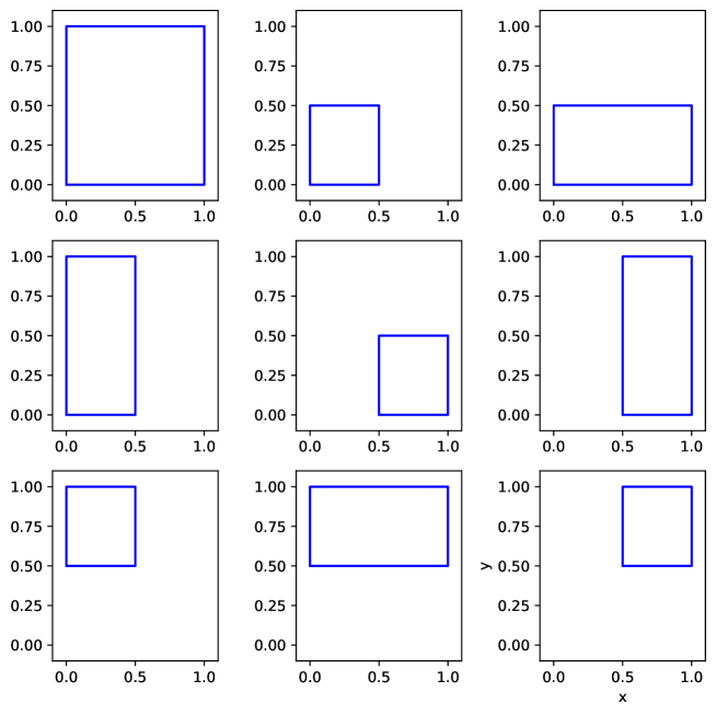
(a)

Figure 1: Geometries used for training

.

2.3 Network’s Complexity

Every $J$ iterations of the classical iterative method is followed by one application of $\mathcal{N}$. As the network’s input is a vector of fixed dimension, each evaluation of the Network on a single data point is of constant computational and memory complexity. As a result, for a sparse (and band-limited) linear system of order $N$, the complexity of each iteration involving $\mathcal{N}$ in (2.3) is $O(N)$ for both memory and computational complexity.

3 Numerical simulations

We compare the performance of HINTS (2.3) for four different models:

1. $\mathcal{N}^{masked}$ is given by (2.1) and was trained on geometries in Figure 1(a).

2. $\mathcal{N}^{non-masked}$ is given by (2.2) and was trained on geometries in Figure 1(a).

3. vanilla Deeponet taken from [28] (see A.1) and was trained on $[0,1]^{2}$.

4. ga-vanilla is a naive implementation of geometry-aware Deeponet using CNN (see A.1) that was trained on the geometries in Figure 1(a).

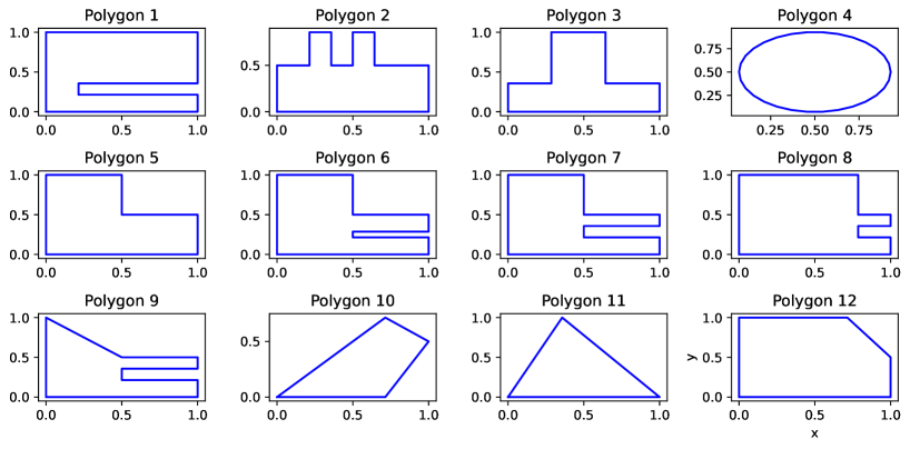
(a)

Figure 2: Tested domains $\Omega$ used in Tables 1, 2 and 3 for solving (1.2).

.

$h$	Method	Model	iter. number
geometry 1
1/57	H-GS(J=40)	$\mathcal{N}^{masked}$	4877
1/57	H-GS(J=40)	ga-vanilla	diverge
1/57	H-GS(J=40)	vanilla	diverge
1/57	H-GS(J=40)	$\mathcal{N}^{non-masked}$	diverge
geometry 2
1/57	H-GS(J=60)	$\mathcal{N}^{masked}$	12000
1/57	H-GS(J=60)	ga-vanilla	diverge
1/57	H-GS(J=60)	vanilla	diverge
1/57	H-GS(J=60)	$\mathcal{N}^{non-masked}$	16000
geometry 3
1/57	H-GS(J=40)	$\mathcal{N}^{masked}$	$2157$
1/57	H-GS(J=40)	ga-vanilla	1616
1/57	H-GS(J=40)	vanilla	$1325$
1/57	H-GS(J=40)	$\mathcal{N}^{non-masked}$	$1381$
geometry 4
1/57	H-GS(J=40)	$\mathcal{N}^{masked}$	$1519$
1/57	H-GS(J=40)	ga-vanilla	diverge
1/57	H-GS(J=40)	vanilla	$813$
1/57	H-GS(J=40)	$\mathcal{N}^{non-masked}$	$764$
geometry 5
1/57	H-GS(J=40)	$\mathcal{N}^{masked}$	$1620\pm 170$
1/57	H-GS(J=40)	ga-vanilla	diverge
1/57	H-GS(J=40)	vanilla	$1064$
1/57	H-GS(J=40)	$\mathcal{N}^{non-masked}$	$842$
geometry 6
1/57	H-GS(J=40)	$\mathcal{N}^{masked}$	6300
1/57	H-GS(J=40)	ga-vanilla	diverge
1/57	H-GS(J=40)	vanilla	$>$20000
1/57	H-GS(J=40)	$\mathcal{N}^{non-masked}$	7200
geometry 7
1/57	H-GS(J=40)	$\mathcal{N}^{masked}$	10800
1/57	H-GS(J=40)	ga-vanilla	diverge
1/57	H-GS(J=40)	vanilla	diverge
1/57	H-GS(J=40)	$\mathcal{N}^{non-masked}$	8034
geometry 8
1/57	H-GS(J=40)	$\mathcal{N}^{masked}$	2028
1/57	H-GS(J=40)	ga-vanilla	2400
1/57	H-GS(J=40)	vanilla	$1370$
1/57	H-GS(J=40)	$\mathcal{N}^{non-masked}$	$1617$

Table 1: Averaged iteration number statistics for the method (2.3) with HINTS Gauss-Seidel (H-GS) with the geometries in Figure 2(a), $k^{2}=21$, $\alpha=0.3$. The classical Gauss-Seidel iterations are not presented as they diverge.

$h$	Method	Model	iter. number
geometry 9
1/57	H-GS(J=80)	$\mathcal{N}^{masked}$	9700
1/57	H-GS(J=80)	ga-vanilla	diverge
1/57	H-GS(J=80)	vanilla	diverge
1/57	H-GS(J=80)	$\mathcal{N}^{non-masked}$	18500
geometry 10
1/57	H-GS(J=40)	$\mathcal{N}^{masked}$	2500
1/57	H-GS(J=40)	ga-vanilla	diverge
1/57	H-GS(J=40)	vanilla	2450
1/57	H-GS(J=40)	$\mathcal{N}^{non-masked}$	1055
geometry 11
1/57	H-GS(J=80)	$\mathcal{N}^{masked}$	2100
1/57	H-GS(J=80)	ga-vanilla	1770
1/57	H-GS(J=80)	vanilla	$1055$
1/57	H-GS(J=80)	$\mathcal{N}^{non-masked}$	1040
geometry 12
1/57	H-GS(J=40)	$\mathcal{N}^{masked}$	1200
1/57	H-GS(J=40)	ga-vanilla	1000
1/57	H-GS(J=40)	vanilla	940
1/57	H-GS(J=40)	$\mathcal{N}^{non-masked}$	560

Table 2: Averaged iteration number statistics for the method (2.3) with HINTS Gauss-Seidel (H-GS) with the geometries in Figure 2(a), $k^{2}=21$, $\alpha=0.3$. The classical Gauss-Seidel iterations are not presented as they diverge.

$h$	Method	Model	GMRES iter.num.	Deeponet iter. num.
geometry 1
1/224	GMRES	-	27120	-
1/224	H-GMRES(m=30,J=10)	$\mathcal{N}^{masked}$	11400	130
1/224	H-GMRES(m=30,J=10)	vanilla	11000	120
1/224	H-GMRES(m=30,J=10)	$\mathcal{N}^{non-masked}$	24797	273
geometry 2
1/224	GMRES	-	19416	-
1/224	H-GMRES(m=30,J=10)	$\mathcal{N}^{masked}$	8500	90
1/224	H-GMRES(m=30,J=10)	vanilla	25800	285
1/224	H-GMRES(m=30,J=10)	$\mathcal{N}^{non-masked}$	7200	70
geometry 4
1/224	GMRES	-	21570	-
1/224	H-GMRES(m=30,J=10)	$\mathcal{N}^{masked}$	5300	57
1/224	H-GMRES(m=30,J=10)	vanilla	3824	42
1/224	H-GMRES(m=30,J=10)	$\mathcal{N}^{non-masked}$	4490	48
geometry 6
1/224	GMRES	-	17816	-
1/224	H-GMRES(m=30,J=10)	$\mathcal{N}^{masked}$	8814	96
1/224	H-GMRES(m=30,J=10)	vanilla	13400	147
1/224	H-GMRES(m=30,J=10)	$\mathcal{N}^{non-masked}$	13079	144
geometry 7
1/224	GMRES	-	18426	-
1/224	H-GMRES(m=30,J=10)	$\mathcal{N}^{masked}$	8800	96
1/224	H-GMRES(m=30,J=10)	vanilla	16500	190
1/224	H-GMRES(m=30,J=10)	$\mathcal{N}^{non-masked}$	15300	170
geometry 9
1/224	GMRES	-	14616	-
1/224	H-GMRES(m=30,J=10)	$\mathcal{N}^{masked}$	8800	100
1/224	H-GMRES(m=30,J=10)	vanilla	14600	160
1/224	H-GMRES(m=30,J=10)	$\mathcal{N}^{non-masked}$	9900	108
geometry 11
1/224	GMRES	-	16257	-
1/224	H-GMRES(m=30,J=10)	$\mathcal{N}^{masked}$	5500	60
1/224	H-GMRES(m=30,J=10)	vanilla	4140	45
1/224	H-GMRES(m=30,J=10)	$\mathcal{N}^{non-masked}$	3830	42

Table 3: Averaged iteration number statistics for the method (2.3) with HINTS GMRES (H-GMRES) with the geometries in Figure 2(a), $k^{2}=21$, $\alpha=0.3$.

Our tested geometries for problem (1.2) are presented in Figure 2(a). We discretize each tested domain with a higher resolution than the resolution used for training, $N=15$. We solve (1.4) using 2.3 with a random function $f$, sampled from another distribution than the one used for training ( $f$ has been generated as a vector from a normal distribution with mean ten and variance 10.). Since the neural network operates on the error terms only, the distribution of $f$ does not affect the hybrid scheme’s robustness. We compare our method with both Gauss-Seidel iterations (see Table 1) and GMRES iterations (see Table 3). The main advantage of Gauss-Seidel (GS) is that, for sparse systems, it has linear complexity in both memory and computational time. However, GS does not always converge for the non-definite cases in our examples. We will show that Hints-GS converges even when plain Gauss-Seidel iterations diverge. GMRES’s main advantage is proven convergence for any non-singular matrix, while its major drawback is memory complexity. For (not necessarily sparse) linear equations with $N$ equations (i.e., corresponding matrix $A\in\mathbb{C}^{N\times N}$), the iteration complexity of GMRES after $n$ iterations is $O(Nn^{2})$ and the memory complexity is $O(N)$. A possible remedy is the restarted GMRES method, GMRES(m), whose memory complexity reduces to $O(mn)$ independently of the number of iterations but with a possible degradation of convergence rates. We will show that combining GMRES inside (2.3) yields a more efficient method in terms of both time and computational complexity.

It is worth noting that, even when Gauss-Seidel iterations diverge, they are still known to reduce high-frequency errors throughout the iterations. Therefore, Hints-GS highlights the capability of HINTS to effectively control low-frequency modes.

We use the following schemes for comparisons as $\mathcal{H}$ in (2.3): GMRES, Gauss-Seidel (GS) , Hints-GS, Hints-GMRES, see subsection 1.3. Multiple computations were performed, and we show the mean number of iterations required. $k>0$ is the wavenumber in the Helmholtz equation, $h=dx=dy$ is the discretization size, and $J$ is the skip factor in (2.3) for how often the neural network $\mathcal{N}$ (Deeponet) is called.

Remark 3.1.

One of the highlights of [16] was the generalization capability of the vanilla Deeponet on a difficult obstacle problem. We also performed experiments of problem (1.2) on an obstacle problems with $\Omega=[0,1]^{2}\setminus[0.25,0.5]^{2}$ and $\Omega=[0,1]^{2}\setminus[0.25,0.75]^{2}$, and observed the superiority of $\mathcal{N}^{masked}$ on the vanilla Deeponet (see Table 4). We have also performed additional experiments on exterior domains with different shapes of obstacles (see Table 5).

$h$	Method	Model	iter. number
obstacle 1
1/57	Gauss-Seidel	-	diverge
1/57	H-GS(J=40)	vanilla	18000
1/57	H-GS(J=40)	$\mathcal{N}^{masked}$	8000
obstacle 2
1/57	Gauss-Seidel	-	10600
1/57	H-GS(J=100)	vanilla	$>$20000
1/57	H-GS(J=100)	$\mathcal{N}^{masked}$	3425
obstacle 1
1/224	GMRES	-	21400
1/224	H-GMRES(J=15)	vanilla	diverge
1/224	H-GMRES(J=15)	$\mathcal{N}^{masked}$	14100
obstacle 2
1/224	GMRES	-	6460
1/224	H-GMRES(J=20)	vanilla	12000
1/224	H-GMRES(J=20)	$\mathcal{N}^{masked}$	8100

Table 4: Averaged iteration number statistics for the method (2.3) with HINTS Gauss-Seidel (H-GS) with the geometries in Figure 3, $k^{2}=21$, $\alpha=0.3$.

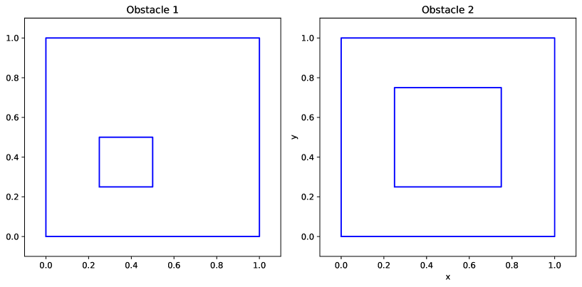
(a)

Figure 3: Tested exterior domains used in Table 4 for solving $\Delta u+k^{2}u=f$. The boundary conditions on the inner boundary are u=0. The boundary conditions on the outer boundary are $\frac{\partial u}{\partial\vec{\nu}}+\sqrt{-1}ku=0$.

$h$	Method	Model	iter. number
1 obstacle
1/57	Gauss-Seidel	-	diverge
1/57	H-GS(J=100)	vanilla	16700
1/57	H-GS(J=100)	$\mathcal{N}^{masked}$	8500
2 obstacles
1/57	Gauss-Seidel	-	diverge
1/57	H-GS(J=100)	vanilla	$>$40000
1/57	H-GS(J=100)	$\mathcal{N}^{masked}$	14500
3 obstacles
1/57	Gauss-Seidel	-	12500
1/57	H-GS(J=200)	vanilla	8300
1/57	H-GS(J=200)	$\mathcal{N}^{masked}$	8500
1 obstacle
1/224	GMRES	-	32100
1/224	H-GMRES(m=30,J=15)	vanilla	10575
1/224	H-GMRES(m=30,J=15)	$\mathcal{N}^{masked}$	16480
2 obstacles
1/224	GMRES	-	18000
1/224	H-GMRES(m=30,J=15)	vanilla	14193
1/224	H-GMRES(m=30,J=15)	$\mathcal{N}^{masked}$	15810
3 obstacles
1/224	GMRES	-	8600
1/224	H-GMRES(m=30,J=15)	vanilla	13343
1/224	H-GMRES(m=30,J=15)	$\mathcal{N}^{masked}$	16717

Table 5: Averaged iteration number statistics for the method (2.3) with HINTS Gauss-Seidel (H-GS) with the geometries in Figure 4, $k^{2}=21$, $\alpha=0.3$.

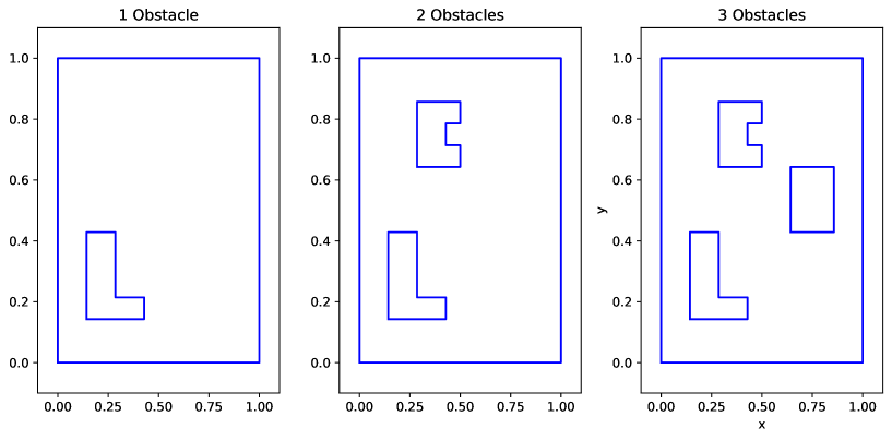
(a)

Figure 4: Tested exterior domains used in Table 5 solving $\Delta u+k^{2}u=f$. The boundary conditions on the inner boundaries are u=0. The boundary conditions on the outer boundary are $\frac{\partial u}{\partial\vec{\nu}}+\sqrt{-1}ku=0$.

3.1 Observations from Tables 1, 2, 3, 4,5

,

We have demonstrated multiple examples with complex geometries for which HINTS with vanilla method fails, while our network succeed. This confirms the necessity of the new models $\mathcal{N}^{masked},\mathcal{N}^{non-masked}$ we presented. In particular, in terms of convergence capability, our new models outperforms the vanilla model. Yet, we mention that the geometry transferability of the vanilla still perform robustly on many domains including non-rectangular ones (geometries 3,4,5,8), and in many cases provide similar or slightly better convergence rates to that of our the geometry aware models.

In almost all tests ga-vanilla obtained the worse results, implying that a naive extension of the vanilla model does not work and more sophisticated approach was required.

When the domain’s boundary contains abrupt changes (cracks/bumps/hole), geometries 1,2,6,7,9, $\mathcal{N}^{masked}$ performed better then all methods. In cases for which vanilla outperformed $\mathcal{N}^{masked}$, $\mathcal{N}^{non-masked}$ outperformed $\mathcal{N}^{masked}$, with an exception for H-GMRES for geometry 1.

In almost all cases we tested there is correlation between HINTS’ performance with different methods (GS,GMRES). Yet, the method used inside HINTS and the corresponding parameters can violate this correlation (e.g. Table 5). In more details, the experiments with the geometries in Figure 4 shows that with GS, $\mathcal{N}^{masked}$ outperforms the vanilla method significantly, whereas for the same problem with GMRES (J=15) vanilla method is better. Yet, for different parameter $J=5$ H-GMRES with vanilla diverged while it did converged with $\mathcal{N}^{masked}$.

We can tell that the idea of extending a function outside its domain to be 0, as suggested in [16] can indeed provide robust results for different domains as long as the domain does not contain abrupt changes (narrow cracks, holes). In these problematic scenarios our masked model can overcome this limit.

Based on our results we suggest to a potential user which cannot use CNN operations to hold both $\mathcal{N}^{masked}$ and $\mathcal{N}^{non-masked}$. Further study on unifying these networks is left for a future research.

Remark 3.2.

The running times of (2.3) can differ for different types of computers. There is room for additional improvement of (2.3) as we did not use a GPU and did not exploit a parallel computation of batched data during inference. In our machine H-GS with higher resolutions than $1/57$ is either very slow or diverges and therefore we switched to GMRES to obtain faster CPU time.

4 Conclusions, Remarks and further research

We have constructed a novel architecture for preconditioning linear equations, which is aware of the geometry of the problem. We showed evidence by numerical examples that our network remains a robust preconditioner for problems with different geometries without any fine-tuning procedure and outperforms existing SOTA methods for tackling similar problems. Another advantage of our proposed network is that is non-convolutional and therefore can be generalized to non-rectangular grids and point-clouds.

We demonstrated our network on a complex Helmholtz equation with complex boundary conditions, which are hard to solve due to non-definiteness or non-symmetry, and on an obstacle problem.

In future work, we intend to generalize our network to include more attention layers and, with the availability of more advanced hardware, to train the network on a larger number of geometries.

Another possible extension is to modify the neural network so that it is invariant under domain translations, as the PDE is.

Funding

The work was supported by the US–Israel Bi-national Science Foundation (BSF) under grant # 2020128.

Declaration of competing interest

The authors declare that they have no known competing financial interests or personal relationships that could have appeared to influence the work reported in this paper.

Data availability

https://github.com/idanv87/convnet.git

Appendix A

A.1 The Networks

For vanilla deeponet, trained on a single domain $[0,1]^{2}$, we employ the architecture in [28, page 37]. The branch net is a combination of a 2D CNN (input dimension $15\times 15$, number of channels [1, 40, 60, 100], kernel size $3\times 3$, stride 2) and dense NN (dimension [100, 80, 80]) with Relu activation function. The dimension of the dense trunk network is [2, 80, 80, 80] with activation of Tanh.

For the naive geometry-aware deeponet (ga-vanilla), we represent the domain as 2D binary image and pad the values of the function $f$ with zeros in all points outside the domain $f$ is defined. We then use CNN as is the vanilla deeponet whose output is concatenated and fed into dense NN (dimension [200, 80, 80]), resulting in the branch. The dimension of the trunk network is [2, 80, 80, 80] with the activation of Tanh.

A.2 Data generation and training

We fix $k^{2}=21$ in (1.4). The vanilla network is trained over 300 solutions of (1.4) in $[0,1]^{2}$ discretized uniformly with $h=\frac{1}{15}$. The solutions are obtained by taking $f$ to be 300 Gaussian random fields (2.4). The equations are solved using standard second-order finite difference method. The network ga-vanilla is trained on the same data used to train $\mathcal{N}^{masked}$, see subsection 2.2.

We trained the networks using Pytorch for 1000 epochs with a batch size of 64, and the initial learning rate 1e-4 decreased by 0.5 at the final epochs.

References

- [1]
- [2] Alciatore, D. and Miranda, R., 1995. A winding number and point-in-polygon algorithm. Glaxo Virtual Anatomy Project Research Report, Department of Mechanical Engineering, Colorado State University.
- [3] Baker, A.H., Jessup, E.R. and Manteuffel, T., 2005. A technique for accelerating the convergence of restarted GMRES. SIAM Journal on Matrix Analysis and Applications, 26(4), pp.962-984.
- [4] Dolean, V., Jolivet, P. and Nataf, F., 2015. An introduction to domain decomposition methods: algorithms, theory, and parallel implementation. Society for Industrial and Applied Mathematics.
- [5] Alexandre Ern, Jean-Luc Guermond. Finite Elements II: Galerkin Approximation, Elliptic and Mixed PDEs. Springer, 2021, 10.1007/978-3-030-56923-5 . hal-03226050
- [6] Ernst, O.G. and Gander, M.J., 2011. Why it is difficult to solve Helmholtz problems with classical iterative methods. Numerical analysis of multiscale problems, pp.325-363.
- [7] Gander, M.J., Graham, I.G. and Spence, E.A., 2015. Applying GMRES to the Helmholtz equation with shifted Laplacian preconditioning: what is the largest shift for which wavenumber-independent convergence is guaranteed?. Numerische Mathematik, 131(3), pp.567-614.
- [8] Gander, M.J. and Zhang, H., 2019. A class of iterative solvers for the Helmholtz equation: Factorizations, sweeping preconditioners, source transfer, single layer potentials, polarized traces, and optimized Schwarz methods. Siam Review, 61(1), pp.3-76.
- [9] Gander, M.J., Magoules, F. and Nataf, F., 2002. Optimized Schwarz methods without overlap for the Helmholtz equation. SIAM Journal on Scientific Computing, 24(1), pp.38-60.
- [10] Gander, M.J., 2006. Optimized schwarz methods. SIAM Journal on Numerical Analysis, 44(2), pp.699-731.
- [11] Gladstone, R.J., Rahmani, H., Suryakumar, V., Meidani, H., D’Elia, M. and Zareei, A., 2024. Mesh-based GNN surrogates for time-independent PDEs. Scientific Reports, 14(1), p.3394.
- [12] Goswami, S., Kontolati, K., Shields, M.D. and Karniadakis, G.E., 2022. Deep transfer operator learning for partial differential equations under conditional shift. Nature Machine Intelligence, 4(12), pp.1155-1164.
- [13] He, J., Koric, S., Kushwaha, S., Park, J., Abueidda, D. and Jasiuk, I., 2023. Novel DeepONet architecture to predict stresses in elastoplastic structures with variable complex geometries and loads. Computer Methods in Applied Mechanics and Engineering, 415, p.116277.
- [14] He, J., Kushwaha, S., Park, J., Koric, S., Abueidda, D. and Jasiuk, I., 2024. Sequential Deep Operator Networks (S-DeepONet) for predicting full-field solutions under time-dependent loads. Engineering Applications of Artificial Intelligence, 127, p.107258.
- [15] He, J., Koric, S., Abueidda, D., Najafi, A. and Jasiuk, I., 2024. Geom-DeepONet: A Point-cloud-based Deep Operator Network for Field Predictions on 3D Parameterized Geometries. arXiv preprint arXiv:2403.14788.
- [16] Kahana, A., Zhang, E., Goswami, S., Karniadakis, G., Ranade, R. and Pathak, J., 2023. On the geometry transferability of the hybrid iterative numerical solver for differential equations. Computational Mechanics, 72(3), pp.471-484.
- [17] Kashefi, A., Rempe, D. and Guibas, L.J., 2021. A point-cloud deep learning framework for prediction of fluid flow fields on irregular geometries. Physics of Fluids, 33(2).
- [18] Kopanicakova, A. and Karniadakis, G.E., 2024. Deeponet based preconditioning strategies for solving parametric linear systems of equations. arXiv preprint arXiv:2401.02016.
- [19] Lions, P.L., 1990, March. On the Schwarz alternating method. III: a variant for nonoverlapping subdomains. In Third international symposium on domain decomposition methods for partial differential equations (Vol. 6, pp. 202-223). Philadelphia: SIAM
- [20] Lu, L., Jin, P., Pang, G., Zhang, Z. and Karniadakis, G.E., 2021. Learning nonlinear operators via DeepONet based on the universal approximation theorem of operators. Nature machine intelligence, 3(3), pp.218-229.
- [21] Rahaman, N., Baratin, A., Arpit, D., Draxler, F., Lin, M., Hamprecht, F., Bengio, Y. and Courville, A., 2019, May. On the spectral bias of neural networks. In International conference on machine learning (pp. 5301-5310). PMLR.
- [22] Raza, S. and Ding, C., 2019. Progress in context-aware recommender systems—An overview. Computer Science Review, 31, pp.84-97.
- [23] Vaswani, A., Shazeer, N., Parmar, N., Uszkoreit, J., Jones, L., Gomez, A.N., Kaiser, Ł. and Polosukhin, I., 2017. Attention is all you need. Advances in neural information processing systems, 30.
- [24] Saad, Y. and Schultz, M.H., 1986. GMRES: A generalized minimal residual algorithm for solving nonsymmetric linear systems. SIAM Journal on scientific and statistical computing, 7(3), pp.856-869.
- [25] Yin, M., Charon, N., Brody, R., Lu, L., Trayanova, N. and Maggioni, M., 2024. Dimon: Learning solution operators of partial differential equations on a diffeomorphic family of domains. arXiv preprint arXiv:2402.07250.
- [26] Zou, Q., 2023. GMRES algorithms over 35 years. Applied Mathematics and Computation, 445, p.127869.
- [27] Zhang, S., Yao, L., Sun, A. and Tay, Y., 2019. Deep learning based recommender system: A survey and new perspectives. ACM computing surveys (CSUR), 52(1), pp.1-38.
- [28] E. Zhang, A. Kahana, A. Kopanicakova, E. Turkel, R. Ranade, J. Pathak and G.E. Karniadakis ”Blending Neural Operators and Relaxation Methods in PDE Numerical Solvers” accepted Nature Machine Intelligence
- [29] Zhu, M., Feng, S., Lin, Y. and Lu, L., 2023. Fourier-DeepONet: Fourier-enhanced deep operator networks for full waveform inversion with improved accuracy, generalizability, and robustness. arXiv preprint arXiv:2305.17289.