An efficient, adaptive solver for accurate simulation of multicomponent shock-interface problems for thermally perfect species

Abstract

A second-order-accurate finite volume method, hybridized by blending an extended double-flux algorithm and a traditionally conservative scheme, is developed. In this scheme, hybrid convective fluxes as well as hybrid interpolation techniques are designed to ensure stability and accuracy in the presence of both material interfaces and shocks. Two computationally efficient approaches, extended from the original double-flux model, are presented to eliminate the well-known ”pressure oscillation” phenomenon at material interfaces observed with the traditional conservative scheme. Numerous verfication simulations confirm that the method is capable of handling multi-dimensional shock-interface problems reliably and efficiently, even in the presence of viscous and reactive terms.

[inst1]organization=Hypersonic Technology Laboratory, National University of Defense Technology, city=Changsha, postcode=410073, country=P.R.China

[inst2]organization=AMROC CFD, addressline=Brookweg 167, city=Oldenburg, postcode=26127, country=Germany

Extension of the the original double-flux model to multicomponent mixtures with thermally perfect species to only one auxillary variable required and with better physical interpretability.

Development of a new hybrid method by blending an extended double-flux algorithm and a standard conservative scheme by utilizing hybrid convective fluxes and interpolation techniques.

Verification and validation of the presented new hybrid solver by extensive one- and multi-dimensional benchmark tests and also some very complex chemically reacting problems

1 Introduction

It is nowadays well established that a fully conservative scheme will usually lead to spurious pressure and velocity oscillations at material interfaces with variable specific heat ratio $\gamma$ when solving the Euler or Navier-Stokes equations in the hyperbolic regime [1, 2, 3, 4]. Earlier works by Karni [2] and Jenny et al. [5] recognized that this pressure oscillation problem is rooted in the numerical averaging or smearing of $\gamma$ across cells. To eliminate this issue, one way is to develop ”sharp-interface” methods, which essentially avoid smearing out $\gamma$ by tracking the propagating material front [4, 6, 7]. One classic method among them was presented by Karni [2] who evolved the original governing equations into a non-conservative formulation by solving additionally the advection equation of one primitive variable. Using this approach, artificial pressure oscillations were perfectly cured and Abgrall [3] later extended this approach to handle strong shocks as well. Besides, there is also a family of non-oscillatory approaches named as the ”Ghost Fluid Method” (GFM) [8, 9, 10, 11], which preserve the interface sharpness by defining a level-set function and using ghost fluid cells to swap information across the interface. The GFM methods combine the advantages of both Eulerian and Langrangian approaches and have been widely used to handle multi-phase fluid problems [12, 13, 14].

Another approach is to control the pressure fluctuation by artificially remedying the solution of the conservative total energy. One of the typical strategies was put forward by Jenny et al. [5] who implemented a simple correction onto the total energy per volume, which preserved the interface free of oscillations. Although during this process the scheme conservation is inevitably lost, numerical stability and convergence issues have not been reported [5, 15, 16, 17].

However, all the methods mentioned above were tailored for calorically perfect gases whose thermodynamic properties, like $C_{p},C_{v}$ and $\gamma$, do not change intricately with the local temperature, and thus formerly mentioned strategies, like discretizing an additional primitive equation or simple energetic correction, could work. Note that for calorically perfect gases, it is generally not necessary to consider the possible issue of the schemes in the presence of shock waves since the specific heat ratio $\gamma$ in this model remains constant across shocks .

In order to consider species with temperature-dependent thermodynamic properties, Abgrall proposed the original ”double-flux” model [18], which was subsequently improved by Billet and Abgrall [15]. This approach basically followed the strategy of a non-conservative energetic correction procedure but was explicitly tailored for thermally perfect gases. The concept was to define two sets of numerical fluxes at every edge, for respectively its left- and right-adjacent cell such that a cell could evolve purely based upon its own thermodynamic properties, i.e. the thermodynamic properties got effectively frozen during the cell-based time evolution. Apparently, the original double-flux model was non-conservative and could not handle strong shocks directly because inconsistent fluxes do not guarantee convergence to the correct weak solution. The methodology of the original double-flux model as well as its deficiency will be further discussed later in Section Extended double-flux method.

The double-flux approach by Billet and Agbrall [15] has been used subsequently to simulate complex, real-world mixing and combustion problems, as done in [16, 19, 20]. In recent years, there have been also some efforts to further develop the original method. For example, Houim and Kuo [16] extended the original method of second order accuracy to the high-order WENO scheme. Lv and Ihme [17] as well as Johnson and Kercher [7] extended it separately to the Discontinuous Galerkin (DG) framework for solving chemically reacting Navier-Stokes equations. The compatibility of the double-flux model with the DG method in the presence of viscous terms has recently been analyzed [21]. It has also been reported that the oscillations in addition create spurious temperature spikes and species errors [22, 23], which may lead to significant numerical artifacts.

In this paper, based on the double-flux model, we design a hybrid solver containing both hybrid fluxes and hybrid interpolations, and thus ensure convergence towards the correct weak solution. Specifically, an extended double-flux scheme is developed and used in regions where the pressure is smooth, including the material interfaces, while a traditionally conservative scheme is implemented especially for shock capturing. For hybridization switching, many works have contributed to the accurate and efficient recognition of discontinuities within smooth solutions by using an explicit shock sensor [24]-[25]. A comprehensive comparison and summary can be found in [26]. For example, Hill and Pullin [27] developed and combined the tuned central difference (TVD) scheme with the WENO method for compressible large-eddy simulation. In their hybridization methdology, to limit the usage of WENO scheme to shocks, a scaled criterion of the smoothness indicator over the WENO candidate stencils was employed for determination of the nodal flux $\hat{f}_{j+1/2}$. Ziegler et al. [28] then improved the shock-detection technique by applying the Liu entropy condition calculated by a Roe-averaged approximate Riemann solver. Besides that, instead of explicitly switching between the central-difference and upwind schemes, Jiang et al [29] used a multi-dimensional optimal order detection (MOOD) approach [30, 31, 32] by distinguishing the ”problematic” cells with the usage of physical and numerical admissibility conditions in order to implement in these cells an upwind discretization. In the present study, since both of the utilized fluxes are calculated based on a monotonicity preserving upwind scheme, the choice of shock sensor is less crucial for stable, accurate shock-interface simulation. Therefore, the normalised second derivative of pressure, that has been used in the classical artificial viscosity method [33], is employed.

Our codes are verified to be capable of handling complex scenarios with the presence of both material interfaces and shock discontinuities, as well as their complicated interaction. Generally, our improved strategy is more efficient and straightforward to implement than enlarging the whole equation system and requires just a minor modification on the total energy and minimal additional coding efforts.

2 Governing equations and numerical methodology

2.1 Chemically reacting compressible Navier-Stokes equations

In this paper, we consider finite volume discretizations of the compressible multicomponent Navier-Stokes system to describe the multi-dimensional reacting flows with detailed chemical kinetics. Soret and Dufour effects, external body forces (e.g. the gravity) and radiant heat transfer are all neglected. The basic equation reads

$$\frac{\partial\boldsymbol{U}}{\partial t}+\frac{\partial\boldsymbol{F}}{\partial x}+\frac{\partial\boldsymbol{G}}{\partial y}=\frac{\partial\boldsymbol{F^{v}}}{\partial x}+\frac{\partial\boldsymbol{G^{v}}}{\partial y}+\boldsymbol{S_{\text{chem}}}\;,$$ (1)

where the state vector $\boldsymbol{U}$ of the conservative variables and the convective flux vectors $\boldsymbol{F}$, $\boldsymbol{G}$ read

$$\boldsymbol{U}=\begin{pmatrix}\rho_{1}\\ \vdots\\ \rho_{N_{sp}}\\ \rho u\\ \rho v\\ \rho E\end{pmatrix},\quad\boldsymbol{F}=\begin{pmatrix}\rho_{1}u\\ \vdots\\ \rho_{N_{sp}}u\\ \rho u^{2}+p\\ \rho uv\\ (\rho E+p)u\end{pmatrix},\quad\boldsymbol{G}=\begin{pmatrix}\rho_{1}v\\ \vdots\\ \rho_{N_{sp}}v\\ \rho uv\\ \rho v^{2}+p\\ (\rho E+p)v\end{pmatrix}$$ (2)

and the viscous fluxes $\boldsymbol{F^{v}}$, $\boldsymbol{G^{v}}$ read

$$\boldsymbol{F^{v}}=\begin{pmatrix}-J_{x,1}\\ ...\\ -J_{x,N_{sp}}\\ \tau_{xx}\\ \tau_{xy}\\ u\tau_{xx}+v\tau_{xy}-q_{x}\\ \end{pmatrix},\quad \boldsymbol{G^{v}}=\begin{pmatrix}-J_{y,1}\\ ...\\ -J_{y,N_{sp}}\\ \tau_{yx}\\ \tau_{yy}\\ u\tau_{yx}+v\tau_{yy}-q_{y}\\ \end{pmatrix}.$$ (3)

Here, $\boldsymbol{J_{k}}$ denotes the molecular diffusion flux vectors of species $k$ with components

$$J_{x,k} =\rho Y_{k}\left[\left(-\frac{1}{X_{k}}\right)D_{k}\left(\frac{\partial X_{i}}{\partial x}+\frac{X_{k}-Y_{k}}{p}\frac{\partial p}{\partial x}\right)\right],$$ (4)

$$J_{y,k} =\rho Y_{k}\left[\left(-\frac{1}{X_{k}}\right)D_{k}\left(\frac{\partial X_{i}}{\partial y}+\frac{X_{k}-Y_{k}}{p}\frac{\partial p}{\partial y}\right)\right].$$

The viscous stress tensor $\boldsymbol{\tau}$ is given by

$$\tau_{xx} =\mu\left(2\frac{\partial u}{\partial x}-\frac{2}{3}\left(\frac{\partial u}{\partial x}+\frac{\partial v}{\partial y}\right)\right),$$ (5)

$$\tau_{xy} =\mu\left(\frac{\partial u}{\partial y}+\frac{\partial v}{\partial x}\right),$$

$$\tau_{yy} =\mu\left(2\frac{\partial v}{\partial y}-\frac{2}{3}\left(\frac{\partial u}{\partial x}+\frac{\partial v}{\partial y}\right)\right)$$

and the heat flux vector $\boldsymbol{q}$ is determined by

$$q_{x}=\sum_{k=1}^{N_{sp}}J_{x,k}h_{k}-\lambda\frac{\partial T}{\partial x},\quad q_{y}=\sum_{k=1}^{N_{sp}}J_{y,k}h_{k}-\lambda\frac{\partial T}{\partial y},$$ (6)

where $h_{k}$ is the specific enthalpy of the $k$-th species and its contribution to the total enthalpy $h$ is expressed as

$$h=\sum_{k=1}^{N_{sp}}Y_{k}h_{k}.$$ (7)

Mixture properties are determined from the pure species properties and are re-evaluated every numerical time step. The molecular diffusion coefficients $D_{k}$ are obtained with the multi-species diffusion model considering the pressure effect

$$D_{k}=\frac{1-X_{k}}{\sum_{j\neq k}^{N_{sp}}(X_{k}/D_{kj})}\frac{p_{0}}{p},$$ (8)

where $p_{0}$ is the ambient pressure. The mixture-averaged viscosity $\mu$ is given by the semi-empirical formula due to Wilke [34] and modified by Bird et al [35]. For the mixture-averaged thermal conductivity $\lambda$, a combination averaging formula [36] was used

$$\lambda=\frac{1}{2}\left(\sum_{k=1}^{N_{sp}}X_{k}\lambda_{k}+\frac{1}{\sum_{k=1}^{N_{sp}}X_{k}/\lambda_{k}}\right).$$ (9)

The reaction source term $\boldsymbol{S_{\text{chem}}}$ in Eq. Chemically reacting compressible Navier-Stokes equations reads

$$\boldsymbol{S_{\text{chem}}}=\left(\dot{\omega}_{1},\ldots,\dot{\omega}_{N_{sp}},0,0,0\right)^{T}.$$ (10)

The chemical production rates $\dot{\omega}_{k}\left(\rho_{1},\ldots,\rho_{N_{sp}},T\right)$ are derived from a reaction mechanism that consists of $J$ chemical reactions

$$\sum_{k=1}^{N_{sp}}\nu_{jk}^{f}S_{k}\rightleftharpoons\sum_{k=1}^{N_{sp}}\nu_{jk}^{r}S_{k},\quad j=1,\ldots,J,$$ (11)

where $\nu_{ji}^{f}$ and $\nu_{ji}^{r}$ are the stoichiometric coefficients of species $S_{k}$ appearing as a reactant and as a product. The entire molar production rate of species $S_{k}$ per unit volume is then given by

$$\dot{\omega}_{k}=\sum_{j=1}^{J}\left(\nu_{jk}^{r}-\nu_{jk}^{f}\right)\left[k_{j}^{f}\prod_{k=1}^{N_{sp}}\left(\frac{\rho_{k}}{W_{k}}\right)^{\nu_{jk}^{f}}-k_{j}^{r}\prod_{k=1}^{N_{sp}}\left(\frac{\rho_{k}}{W_{k}}\right)^{\nu_{jk}^{r}}\right],\quad k=1,\ldots,N_{sp},$$ (12)

with $k_{j}^{f}(T)$ and $k_{j}^{r}(T)$ denoting the forward and backward reaction rate of each chemical reaction, respectively. Each forward reaction rate is given by an Arrhenius formula and the backward reaction rates is calculated from the respective chemical equilibrium constant. In the present study, a detailed chemical model with 13 species and 27 reversible reaction steps developed by Burke et al. [37] was employed.

For closure of the above system, we have the ideal gas law which reads

$$p=\rho RT=\sum_{k=1}^{N_{sp}}\rho Y_{k}\frac{RU}{W_{k}}T,$$ (13)

where $R$ is the gas constant and $W_{k}$ is the relative molecular mass of species $k$.

A thermally perfect equation of state is used to determine the total energy per volume $E$ of gas with variable specific heat ratio $\gamma$ dependent on the temperature as

$$E =h-\frac{p}{\rho}+\frac{1}{2}\left({u}^{2}+{v}^{2}\right)$$ (14)

$$=\sum_{k=1}^{N_{sp}}\left(Y_{k}h^{f}_{k0}+Y_{k}\int_{T_{0}}^{T}C_{pk}(s)ds\right)-\frac{p}{\rho}+\frac{1}{2}\left({u}^{2}+{v}^{2}\right).$$

This property is of vital importance for solving chemical non-equilibrium flows, which are typically exposed to large temperature gradients. The specific heat capacity at constant pressure, $C_{pk}$, as well as the partial enthalpy $h_{k}$ of the $k$-th species are determined by the CHEMKIN library.

In contrast, we also write down the equation of state for a calorically perfect gas

$$E_{\text{cal}}=\frac{p}{\gamma-1}+\frac{1}{2}\left({u}^{2}+{v}^{2}\right).$$ (15)

2.2 Numerical schemes

In this section, we present the numerical methodology for solving the multi-dimensional chemically reacting Navier-Stokes equations. An overall second-order-accurate Strang splitting method is employed for decoupling of the transport and reactive parts and thereby ensure computational efficiency and robustness, given by

$$\boldsymbol{U}^{n+1}=\mathcal{S}^{\left(\frac{1}{2}\Delta t\right)}\mathcal{H}^{(\Delta t)}\mathcal{S}^{\left(\frac{1}{2}\Delta t\right)}\left(\boldsymbol{U}^{n}\right),$$ (16)

where $\mathcal{S}$ and $\mathcal{H}$ stand for the time operator of the inhomogeneous ordinary differential part and the homogeneous partial differential part, respectively.

For the homogeneous part, an unsplit finite-volume approach is employed with each volume advanced by accounting for all flux contributions in a single step. In each dimension, a second-order-accurate MUSCL (Monotone Upstream-centered Schemes for Conservation Laws) scheme is employed for discretization of the convective terms and a second-order-accurate central difference scheme for the viscous terms. In the MUSCL reconstruction, determination of the edge value $\boldsymbol{U}_{j\pm 1/2}$ is first achieved by a linear interpolation between the three cells $j-1$, $j$ and $j+1$. Special factors $\Phi_{j\pm 1/2}^{\pm}$, called the slope limiters, are utilized to reconstruct the gradients used for this interpolation to ensure the TVD property and positivity of the species mass fractions:

$$\tilde{U}_{j+\frac{1}{2}}^{L}=U_{j}^{l}+\frac{1}{4}\left[(1-\omega)\Phi_{j-\frac{1}{2}}^{+}\Delta_{j-\frac{1}{2}}+(1+\omega)\Phi_{j+\frac{1}{2}}^{-}\Delta_{j+\frac{1}{2}}\right],$$ (17a)

$$\tilde{U}_{j-\frac{1}{2}}^{R}=U_{j}^{l}-\frac{1}{4}\left[(1-\omega)\Phi_{j+\frac{1}{2}}^{-}\Delta_{j+\frac{1}{2}}+(1+\omega)\Phi_{j-\frac{1}{2}}^{+}\Delta_{j-\frac{1}{2}}\right].$$ (17b)

In this present paper, the minmod limiter is applied to ensure calculation stability. Note, that only for $\omega=0$ the following conservation property is satisfied:

$$U_{j}^{l} = \frac{1}{\Delta x}\int_{x_{j-1/2}}^{x_{j+1/2}}\tilde{U}(\xi)d\xi$$ (18)

High-order spatial methods are unstable under the forward-Euler time integration method. The method of lines is therefore a frequently selected approach for the temporal discretization of hyperbolic problems. In this paper, an explicit two-stage strong stability preserving Runge-Kutta method (SSPRK2) of second order time accuracy is employed. Its steps are

$$K_{1} =\Delta tS(t^{n},\boldsymbol{U}^{n}),$$ (19a)

$$K_{2} =\Delta tS(t^{n}+\Delta t,\boldsymbol{U}^{n}+K_{1}),$$ (19b)

$$\boldsymbol{U}^{n+1} =\boldsymbol{U}^{n}+\frac{1}{2}[K_{1}+K_{2}].$$ (19c)

The Riemann solver used in this paper is the HLLC solver [38], which inherently preserves the velocity equilibrium across the material interface after one time step $dt$. The latter is crucially important for developing a new method based on the double-flux model, which will be seen in later sections. Other flux solvers with this property, such as the AUSM⁺ scheme [39], could also be applied. The viscous diffusion terms are evaluated simply by standard second-order-accurate central differences. Each integration of the source term is done with the fourth-order semi-implicit Runge-Kutta method (GRK4A) [40], which is capable of handling the stiffness of the ODEs due to the detailed chemical kinetics.

3 Extended double-flux method

Spurious oscillations will be generated at a material interface when solving the multicomponent Euler or Naiver-Stokes equations with variable specific heat ratio $\gamma$. The double-flux algorithm is an efficient method that is able to preserve the pressure and velocity across a material interface. The approach has been proposed by Abgrall et al. [3, 15] and was later extended to a high-order WENO scheme [16] in the finite difference framework and a discontinuous Galerkin (DG) method [17], respectively. According to the authors’ knowledge, it is the only method that can handle multicomponent flows with arbitrary number of species whose $C_{pi}$ depend on the temperature.

3.1 Methodology

The original double-flux model required the two auxillary variables, $\gamma$ and $\rho h_{0}^{m}$ and was tailored for the JANAF thermodynamic tables. In this section, we improve the algorithm by requiring only one auxillary variable and nevertheless obtain perfect pressure and velocity equilibrium at a material front. Furthermore, we modified the new algorithm to be applicable to the NASA library. Two approaches of the extended double-flux method are presented and compared in Sections Approach A and Approach B, respectively.

To begin with, a material front can be analyzed by using the one-dimensional inviscid Euler equations

$$\frac{\partial(\rho Y_{i})}{\partial t} =-\frac{\partial(\rho Y_{i}u)}{\partial x},$$ (20a)

$$\frac{\partial(\rho u)}{\partial t} =-\frac{\partial(\rho u^{2}+p)}{\partial x}.$$ (20b)

Since $u,p$ are constant across a material front, Eq. Methodology can be reduced to

$$\delta\left(\rho Y_{i}\right) =-\sigma u\Delta\left(\rho Y_{i}\right),$$ (21a)

$$\delta(\rho u) =-\sigma u^{2}\Delta\rho,$$ (21b)

where $\delta$ and $\Delta$ denote the temporal and spatial difference, respectively, and $\sigma={dt}/{dx}$. Summing Eq. Methodology from $i$ = 1 to $N$ together and substituting the result into Eq. Methodology will yield the relation

$$u^{n+1}=u^{n}.$$ (22)

The latter means that the normal velocity $u$ is inherently preserved after one time step before it is contaminated by the pressure fluctuation.

Substituting Eq. Chemically reacting compressible Navier-Stokes equations into the energy equation (where the pressure oscillation originates), we have

$$\delta\left(\sum\rho Y_{i}h_{i0}^{f}\right)+\delta\left(\sum\rho Y_{i}\int_{T_{0}}^{T}C_{pi}(s)ds\right)-\delta\left(p\right)+\delta\left(\frac{1}{2}\rho u^{2}\right)=$$ (23)

$$-\sigma u\left(\Delta\left(\sum\rho Y_{i}h_{i0}^{f}\right)+\Delta\left(\sum\rho Y_{i}\int_{T_{0}}^{T}C_{pi}(s)ds\right)-\Delta\left(p\right)+\Delta\left(\frac{1}{2}\rho u^{2}\right)\right).$$

Due to the presence of the integral term of $C_{pi}(s)$, directly analyzing Eq. Methodology is challenging. A better way is to first reformulate Eq. Methodology by transforming the equation of state of Eq. Chemically reacting compressible Navier-Stokes equations into a familiar expression like Eq. Chemically reacting compressible Navier-Stokes equations. In the original work by Billet and Abgrall [15], they decomposed the integral $\int_{T_{0}}^{T}C_{pi}(s)ds$, i.e., the sensible enthalpy. Each $C_{pi}$ is dependent on the temperature and obtained from the JANAF tables by piecewise linear interpolation. The integral of $C_{pi}$ except from the last temperature interval can be merged into the enthalpy of formation $h_{i0}^{f}$. Then the total enthalpy per volume can be written as

$$h_{i} =h_{i0}^{f}+\sum_{k=1}^{p}\int_{T_{k-1}}^{T_{k}}\left(\alpha_{i}^{k}s+\beta_{i}^{k}\right)\mathrm{d}s+\int_{T_{p}}^{T}\left(\alpha_{i}^{p}s+\beta_{i}^{p}\right)\mathrm{d}s=h_{i0}^{m}+\int_{T_{p}}^{T}\left(\alpha_{i}^{p}s+\beta_{i}^{p}\right)\mathrm{d}s,$$ (24)

where $\alpha_{i}^{k}$, $\beta_{i}^{k}$ are the constants of piecewise linear interpolation. Introducing

$$\overline{C_{pi}} =\frac{a_{i}^{p}}{2}\left(T+T_{p}\right)+b_{i}^{p}$$ (25)

as the equivalent heat capacity at constant pressure of species $i$ at the last temperature interval $\left[T_{p},T\right]$ and using

$$\hat{h}_{i0}^{m} =h_{i0}^{m}-\overline{C_{pi}}T_{p},\quad\overline{\gamma} =\frac{\overline{C_{p}}}{\overline{C_{p}}-R}$$ (26)

the total energy per volume $E$ can be reformulated into

$$E =h_{0}^{m}+\sum_{i=1}^{N}\overline{C_{pi}}Y_{i}(T-T_{p})-\frac{p}{\rho}+\frac{u^{2}}{2}=\hat{h}_{0}^{m}+\sum_{i=1}^{N}\overline{C_{pi}}Y_{i}T-\frac{p}{\rho}+\frac{u^{2}}{2}$$ (27)

$$=\hat{h}_{0}^{m}+\overline{C_{p}}T-\frac{p}{\rho}+\frac{u^{2}}{2}=\hat{h}_{0}^{m}+\frac{p}{\rho(\overline{\gamma}-1)}+\frac{u^{2}}{2}.$$

Substituting Eq. Methodology into the energy equation of the hyperbolic system, we then have

$$\delta\left(\rho\hat{h}_{0}^{m}\right)+p\delta\left(\frac{1}{\overline{\gamma}-1}\right)+\frac{1}{\overline{\gamma}-1}\delta p+\delta\left(\frac{1}{2}\rho u^{2}\right)$$ (28)

$$=- \sigma u\biggl{[}\Delta\left(\rho\hat{h}_{0}^{m}\right)+p\Delta\left(\frac{1}{\overline{\gamma}-1}\right)+\left(\frac{1}{\overline{\gamma}-1}\right)\Delta p+\Delta\left(\frac{1}{2}\rho u^{2}\right)\biggr{]}.$$

In Eq. Methodology, we can analyze that at a material front to avoid pressure fluctuations, one would have to fix the auxillary variables $\rho\hat{h}_{0}^{m}$ and $\overline{\gamma}$ together during the discrete cell marching. In the specific implementation, the gradients of the hyperbolic numerical fluxes at the iterative computation of cell $j$ in each dimension $i$ are thus calculated by

$$\frac{\partial F}{\partial x_{i}}=\frac{\hat{F}\left(\boldsymbol{U}_{j+1/2}^{L},\boldsymbol{U}_{j+1/2}^{R},\hat{\gamma}_{j},(\rho\hat{h}_{0}^{m})_{j}\right)-\hat{F}\left(\boldsymbol{U}_{j-1/2}^{L},\boldsymbol{U}_{j-1/2}^{R},\hat{\gamma}_{j},(\rho\hat{h}_{0}^{m})_{j}\right)}{\Delta x_{i}}.$$ (29)

This implementation is illustrated in Fig. Schematic diagram of cell-based implementation of the double-flux type method.. Due to the potential inconsistency between the numerical fluxes $\hat{F}_{j-1/2}^{L}$ and $\hat{F}_{j-1/2}^{R}$, non-conservation is inevitably found for the energy term.

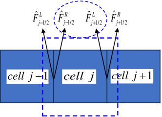
Figure 1: Schematic diagram of cell-based implementation of the double-flux type method.

However, it can be seen that the derivation of the original double-flux model is tedious, mostly attributed to its complex modelling of the specific energy $E$. Although the pressure equilibrium is preserved, one obvious flaw of this method is that the reconstruction of ”mixed enthalpy of formation” $\hat{h}_{0}^{m}$ is void of any physical basis. In the implementation, this method also requires two thermodynamic parameters $\overline{\gamma}$ and $\rho\hat{h}_{0}^{m}$ to be frozen, which complicates the programming and might bring more conservation loss to the energy term.

Having realized the deficiencies of original double-flux model, we found that we could make some improvement to it. In this paper, we modified the algorithm to require only one auxillary variable $\hat{\gamma}$ to eliminate pressure oscillation, by altering the reformulation model of the energy term and greatly simplifying the derivation process. Furtheron, we extended the algorithm to mixtures for which the specific heats $C_{pi}$ are obtained from the NASA database by polynomial interpolation, making it more trivial and straightforward to be used with the CHEMKIN library which has been adopted in most large-scale computational fluid dynamic codes. The concept we employed here is to directly average the enthalpy-based part in the total energy per volume $E$. By utilizing this concept, only one fixed auxillary variable instead of two will be required. We also succeed in preserving the physical fundamentals better since $\hat{\gamma}$ is nothing but the averaged specific heat ratio of the enthalpy-based part.

3.1.1 Approach A

One approach is to directly reformulate the sensible enthalpy contribution in the specific enthalpy, independent of the enthalpy of formation, by introducing $\hat{C}_{pi}$ as an averaged specific heat capacity at constant pressure of species $i$ as

$$\hat{C}_{pi} =\frac{\int_{T_{\text{ref}}}^{T}C_{pi}(s)ds}{T},\quad\hat{C}_{p} =\sum_{i=1}^{N}\hat{C}_{pi}Y_{i},\quad\hat{\gamma} =\frac{\hat{C_{p}}}{\hat{C_{p}}-R},$$ (30)

where $T_{\text{ref}}$ is an arbitrary reference temperature except for 0 K, which is sensible as the polynomial representations are usually not valid down to absolute zero. $\hat{C}_{p}$ is the averaged specific heat capacity at constant pressure and $\hat{\gamma}$ is the averaged specific heat ratio. Note that $\hat{C}_{pi}$ is different from the equivalent heat capacity $\overline{C}_{pi}$ defined in Eq. Methodology as the former one has specific physical meaning. The enthalpy of formation $h_{i0}^{f}$ defined at $T_{\text{ref}}$, on the other hand, is left unchanged.

By doing such, rigorous splitting between the temperature-independent enthalpy of formation and temperature-dependent sensible energy is ensured, and Eq. Chemically reacting compressible Navier-Stokes equations can then be reformulated into a new form resembling the calorically perfect gases, i.e., the ideal gas equation with constant $C_{p}$ and $\gamma$:

$$E=h_{0}^{f}-\frac{1}{\hat{\gamma}-1}\frac{p}{\rho}+\frac{1}{2}({u}^{2}+{v}^{2})$$ (31)

Reformulating and extending Eq. Methodology using the last equation, we obtain

$$\delta\left(\rho h_{0}^{f}\right)+p\delta\left(\frac{1}{\hat{\gamma}-1}\right)+\frac{1}{\hat{\gamma}-1}\delta p+\delta\left(\frac{1}{2}\rho u^{2}\right)$$ (32)

$$=- \sigma u\biggl{[}\Delta\left(\rho h_{0}^{f}\right)+p\Delta\left(\frac{1}{\hat{\gamma}-1}\right)+\left(\frac{1}{\hat{\gamma}-1}\right)\Delta p+\Delta\left(\frac{1}{2}\rho u^{2}\right)\biggr{]}.$$

The conservative enthalpy of formation $\rho h_{0}^{f}$ is mathematically a convex combination of the partial density $\rho Y_{i}$ given by

$$\left(\rho h_{0}^{f}\right)_{t}=-\sum_{i=1}^{K}\left(h_{i0}^{f}\sigma u(\rho Y_{i})_{x}\right)=-\sigma u\sum_{i=1}^{K}\left(\rho Y_{i}h_{i0}^{f}\right)_{x}=-\sigma u\left(\rho h_{0}^{f}\right)_{x}.$$ (33)

Combining Eqs. Methodology and Approach A, the terms regarding the conservative formation of enthalpy and kinetic energy on both sides of Eq. Approach A inherently cancel each other out. Now we have just to freeze $\hat{\gamma}$ during the cell-based evolution $\left[t_{n},t_{n+1}\right]$ to obtain $\delta p=0$. Since we already have $\Delta p=0$, and thus the equilibrium across a material interface will be preserved. Compared to the original double-flux method, the advantage of this new approach is evident: it requires only one auxiliary variable $\hat{\gamma}$, instead of two auxillary variables, $\rho h_{0}^{m}$ and $\gamma$, when modifying the cell-based energy fluxes. This allows for a more concise mathematical derivation and programming procedure.

3.1.2 Approach B

Besides the Approach A, we also present in this paper another more attractive approach by directly modelling the specific enthalpy $h$, so that Eq. Chemically reacting compressible Navier-Stokes equations can be reformulated into a form similar to Eq. Chemically reacting compressible Navier-Stokes equations by defining

$$\hat{C}_{p}=\frac{h}{T},\quad\hat{C}_{p}=\sum_{i=1}^{N}\hat{C}_{pi}Y_{i},\quad\hat{\gamma}=\frac{\hat{C_{p}}}{\hat{C_{p}}-R}.$$ (34)

Eq. Chemically reacting compressible Navier-Stokes equations can then be reformulated into

$$E=\hat{E}_{\text{cal}}\equiv\frac{1}{\hat{\gamma}-1}\frac{p}{\rho}+\frac{1}{2}({u}^{2}+{v}^{2}).$$ (35)

In this approach, we no longer need to manually specify an auxillary constant temperature $T_{\text{ref}}$, which significantly optimized the programming procedure and the issue of non-physical calculation of $\hat{C}_{p}$ got avoided from the root. By conducting a derivation analogous to the one of Eq. Approach A, one can show that the equilibrium of velocity and pressure is strictly guaranteed if $\hat{\gamma}$ is frozen during the cell update.

3.2 Verification and validation

3.2.1 Correctness and efficiency

To verify our presented method and also the correctness of the implementation, we first test the convergence of the extended double-flux method by solving the inviscid Euler equations. However, for thermally perfect gases, the choice of a suitable exact solution is a non-trivial task since the variation of an arbitrary quantity would generally result in variations in $\Delta\gamma$ due to the density, pressure, temperature as well as the species mass fractions coupled by the ideal gas equation. Thus, we turn to an exact solution derived from a problem with trivial variation of $\gamma$

$$\begin{array}[]{c}\rho=h(x-ut)+\rho_{\infty},\\ u=u_{\infty},\\ p=p_{\infty},\end{array}$$ (36)

with $h\left(\psi\right)$ being an arbitrary smooth function. Here, we choose a cosine function.

The entire domain ranges from 0 to 1 and the periodic boundary condition (BC) is employed. In this one-dimensional solution, the wave does not deform because the speed $u$ is constant. This is also known as an entropy wave, which is a linear degenerated wave. In reality, it relates to the contact surfaces or shear layers with only variations in density and constant velocity and pressure.

We use both the traditional conservative scheme and the extended double-flux scheme to calculate this problem, without any use of discontinuity limiters. Unless otherwise specified, all subsequent extended double-flux method verification and validation results have been attained utilizing Approach A. Approach B gives virtually identical results for this problem. Figure Comparison of exact solution with the numerical piece-wise linear solution obtained using the extended double-flux scheme with 32 cells. illustrates that the numerical result obtained with the new extended double-flux scheme is consistent with the exact solution. As listed in Table Convergence study of the extended double-flux method for one-dimensional entropy wave advection., our new method even shows superior performance over the traditional conservative scheme in the $L_{2}$ error of density. While not specifically shown, it also performs similarly in the $L_{1}$ and $L_{\infty}$ error norms as well as errors norms of other quantities. These results show that although some conservation loss is caused inevitably by the double-flux model, numerical errors as well as the convergence order get indeed improved by curing the oscillation issue in the presence of consistent $\gamma$ variation. This test verifies that the proposed extended double-flux scheme works well in this one-dimensional case.

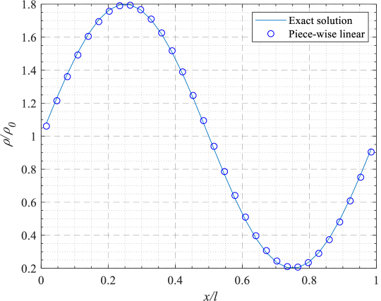
Figure 2: Comparison of exact solution with the numerical piece-wise linear solution obtained using the extended double-flux scheme with 32 cells.

Table 1: Convergence study of the extended double-flux method for one-dimensional entropy wave advection.

	traditional ccheme		extended double-flux method
$h$	$L_{2}$ error	convergece order	$L_{2}$ error	convergece order
1/16	0.05032	-	0.04854	-
1/32	0.01263	1.9940	0.01182	2.0374
1/64	0.003159	1.9991	0.002927	2.0142
1/128	0.0007903	1.9993	0.0007301	2.0032
1/256	0.0001977	1.9991	0.0001823	2.0013

To further verify our scheme in handling multi-dimensional smooth problems, we then extend this problem to two dimensions with the exact solution

$$\begin{array}[]{c}\rho=h(x-ut-vt)+\rho_{\infty},\\ u=u_{\infty},\\ v=v_{\infty},\\ p=p_{\infty}\end{array}$$ (37)

and periodic domain $\left(x,y\right)\in[0,1]\times[0,1]$. Figure Comparison of exact solution with the numerical one obtained using the extended double-flux scheme with 16$\times$16 cells. shows that the numerical solution coincides with the exact solution. A convergence study is conducted to verify the global accuracy of the quasi-conservative scheme in handling multi-dimensional smooth problems. Results in Table Convergence study of the extended double-flux method for two-dimensional entropy wave advection. illustrate that the quasi-conservative solution procedure performed well with second order accuracy in and with slightly higher convergence order when dealing with smooth variations of $\gamma$.

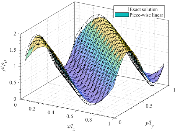
Figure 3: Comparison of exact solution with the numerical one obtained using the extended double-flux scheme with 16$\times$16 cells.

Table 2: Convergence study of the extended double-flux method for two-dimensional entropy wave advection.

	traditional scheme		extended double-flux method
$h$	$L_{2}$ error	convergence order	$L_{2}$ error	convergence order
1/16	0.09896	-	0.09537	-
1/32	0.02533	1.9657	0.02369	2.0088
1/64	0.006354	1.9953	0.005882	2.0103
1/128	0.001591	1.9977	0.001466	2.0036
1/256	0.0003981	1.9988	0.0003661	2.0020

To evaluate the efficiency of the proposed method, we compare the absolute and relative wall cpu time of our presented solver and the original one in AMROC [41], as listed in Table Absolute and relative cpu wall-time consumption of the multi-dimensional entropy waves problem calculated by the fully conservative and extended double-flux schemes. The mesh resolution ranges from 1/16 to 1/512.. It can be observed that although implementing several additional steps like double-flux calculation and energy term modification on the traditional discretization procedure incurs some expenses, the relative cost is always below 10% with the use of from 16 to 512 cells, which is quite acceptable. Moreover, it should be noted that during the calculation of this special case, every cells employed the presented scheme during its discrete evolution while in a real-world computation only a partial region of the whole domain, i.e., the location of the material interfaces or shear layers, should adopt this correction procedure by leveraging the hybrid procedure that will be introduced in Section Hybridization methodology and thus the global computational cost increase would be marginal.

Table 3: Absolute and relative cpu wall-time consumption of the multi-dimensional entropy waves problem calculated by the fully conservative and extended double-flux schemes. The mesh resolution ranges from 1/16 to 1/512.

	1/16	1/32	1/64	1/128	1/256	1/512
$t_{\text{cpu, fc}}$ [s]	0.517	1.423	4.191	18.527	98.924	649.814
$t_{\text{cpu, df}}$ [s]	0.521	1.495	4.413	19.147	106.954	697.568
$\frac{t_{\text{cpu, df}}-t_{\text{cpu, fc}}}{t_{\text{cpu, fc}}}$ [%]	0.774	5.060	5.297	3.346	8.117	7.3490

3.2.2 1-D advection of an inert H2 bubble in O2 gases

To verify the proposed two new approaches, as well as comparing their abilities to resolve the contact surfaces, the advection of an $\ce{H2}$ bubble in $\ce{O2}$ [21] is studied here by solving the inviscid Euler equations with the numerical scheme discussed in Section Numerical schemes. This example illustrates the classic oscillation phenomena when encountering a discontinuous $\gamma$ with a fully conservative scheme, as well as how this is overcome by our new extended double-flux method.

The $\ce{H2}$ bubble is advected with a constant velocity $u_{0}$ = 20 m/s and a uniform pressure $p_{0}$ = $1\times 10^{5}$ Pa. The periodic boundary condition is applied on both left and right boundaries. The initial profiles of mass fraction $Y_{\ce{H2}}$ and temperature $T$ are defined as

$$T(x) =\frac{1}{2}[(1+\Theta)+(1-\Theta)(\tanh(|x-x_{0}|-d)),$$ (38a)

$$Y_{\mathrm{H}_{2}}(x) =\frac{1}{2}[1-\tanh(|x-x_{0}|-d)],$$ (38b)

where the centre of the plateau $x_{0}$, the width of the plateau $d$ and the temperature ratio $\Theta$ are set to 0, 10 and 7, respectively and as in [21]. The physical length of the domain is 50 cm with a uniform grid size $\Delta x$ = 0.2 cm. This test is run with a CFL number of 0.4. The $\ce{H2}$ bubble propagates within the computational domain before the end of the calculation $t_{e}=8500\delta t$ ($\delta t\approx 2.355\times 10^{-7}s$).

The numerical results from the standard conservative scheme and our new presented approaches are depicted in Fig. (a) 1-D inert $\ce{H2}$ bubble advection solved by the extended double-flux solver (df) and the fully conservative scheme (fc) at $t=t_{e}$, (b) local enlargement of Fig. 4(a).. For clarity, we only plot the results obtained with one double-flux approach, since the other performed virtually identically. According to these results, the symmetry of the $\ce{H2}$ bubble as well as the pressure equilibrium are both perfectly preserved by the extended double-flux approach, as seen in the local enlargement of Fig. ‣ (a) 1-D inert $\ce{H2}$ bubble advection solved by the extended double-flux solver (df) and the fully conservative scheme (fc) at $t=t_{e}$, (b) local enlargement of Fig. 4(a).. On the other hand, the fully conservative scheme produces pressure and velocity oscillations clearly visible in Figs. ‣ (a) 1-D inert $\ce{H2}$ bubble advection solved by the extended double-flux solver (df) and the fully conservative scheme (fc) at $t=t_{e}$, (b) local enlargement of Fig. 4(a). and ‣ (a) 1-D inert $\ce{H2}$ bubble advection solved by the extended double-flux solver (df) and the fully conservative scheme (fc) at $t=t_{e}$, (b) local enlargement of Fig. 4(a)..

The conservation loss is recorded during the time span $\left[0,t_{e}\right]$, with the error at time step $n$ expressed as

$$e^{n}=\frac{\left|\psi^{n}-\psi_{0}\right|}{\psi^{n}}=\frac{\left|\Sigma_{j=1}^{N}\left(U^{n}_{j}-U^{0}_{j}\right)\right|}{\Sigma_{j=1}^{N}U^{n}_{j}}$$ (39)

with $U_{j}^{n}=\left[\rho,\rho u,\rho E\right]^{n}$. Both extended double-flux approaches produce a conservation error in mass and momentum within the machine accuracy, as seen in Fig. ‣ Conservation loss by the extended double-flux method with (a) Approach A and (b) Approach B. and ‣ Conservation loss by the extended double-flux method with (a) Approach A and (b) Approach B.. Note that the final total energy loss in this problem is with 0.002913 also significantly smaller as the results in [16], which is achieved thanks to the use of one auxillary variable and the proper reformulation of $E$. For mass and momentum conservation, we note that Approach A gives slightly better performance than Approach B in momentum and with comparable performance in mass conservation. Both approaches have been confirmed to capture material interfaces with no artificial oscillations.

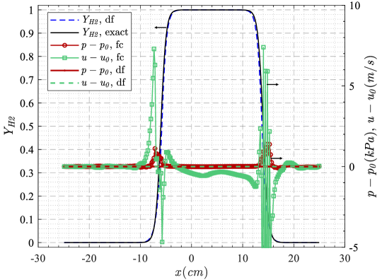
(a)

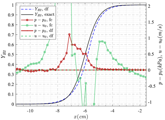
(b)

Figure 4: (a) 1-D inert $\ce{H2}$ bubble advection solved by the extended double-flux solver (df) and the fully conservative scheme (fc) at $t=t_{e}$, (b) local enlargement of Fig. ‣ (a) 1-D inert $\ce{H2}$ bubble advection solved by the extended double-flux solver (df) and the fully conservative scheme (fc) at $t=t_{e}$, (b) local enlargement of Fig. 4(a)..

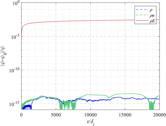
(a)

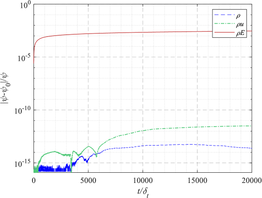
(b)

Figure 5: Conservation loss by the extended double-flux method with (a) Approach A and (b) Approach B.

4 An efficient, adaptive solver for simulation of shock-interface interaction

In spite of our efforts, the inherent conservation concerns accompanied with the extended double-flux method remain an issue. Hence, we have designed an explicit hybrid methodology that ensures correct shock capturing nevertheless. In addition, we have incorporated a highly efficient adaptive mesh refinement (AMR) technique into the overall solver.

4.1 Hybridization methodology

In compressible flows, shock waves are ubiquitous, e.g., in shock bubble interaction, shock induced combustion or detonation. In that respect, a fully conservative shock capturing method is usually preferred under those circumstances to make sure one obtains the correct weak solution. Using a non-conservative scheme like the double-flux method, on the other hand, is generally not a good choice because it might generate huge numerical artifacts by producing an unphysical shock. To remedy this deficiency, we apply hybridized numerical fluxes in the present study by combining the fully conservative shock-capturing scheme and the quasi-conservative extended double-flux method.

To achieve this, we utilize the normalised pressure curvature [27] as a shock sensor

$$S_{i} =\frac{\left|\bar{p}_{i-1}-2\bar{p}_{i}+\bar{p}_{i+1}\right|}{\bar{p}_{i-1}+2\bar{p}_{i}+\bar{p}_{i+1}}.$$ (40)

This normalized sensor is generally resolution independent and hence directly compatible with the local grid refinement of the AMR technique employed. The working procedure is as follows and summarized in Algorithm Hybridization methodology. Before time marching each computational cell, the sensor value $S_{i}$ is calculated to determine which scheme (conservative or non-conservative) is selected. Once $S_{i}$ exceeds a prescribed threshold $S_{i}^{t}$, the double-flux solver will reduce back to the traditional conservative solver by jumping over the frozen and flux correction procedures. If not, a quasi-conservative scheme (aka the extended double-flux ) would be applied on this cell with the use of either Approach A or B. After that, a correction procedure is implemented to update the thermodynamic quantities as well as the total energy $\rho E$. Determination of the threshold $S_{i}^{t}$ is naturally problem-related, which is a common issue of hybrid methods, cf. [28]. In most occasions, they can be resolved separately with the use of our presented hybrid solver. For phenomena like the detonation wave in whose structure the shock and reaction fronts are coupled closely, it should be and also is resolved simply by the conservative scheme since this phenomenon is dominated more by shock compression instead of physical diffusion and thereby ensuring the correct weak solution is critical.

The extended double-flux scheme is a Godunov-type scheme and is usually extended to higher order accuracy in space and time [15]. For the MUSCL-TVD scheme employed in this work, we interpolate the primitive variables onto the cell edges, which is computationally efficient and preferred in most occasions. However, as reported in [16], this interpolation technique may generate oscillations near shock fronts. Although this can be tackled to some degree by decomposing the interpolation variables onto the characteristic fields globally, the entire computational load would be tremendously increased and also the double-flux algorithms would become much more involved [16]. Consequently, in this paper, we also combine the selection of interpolation variables into our current hybrid solver: we decompose the conservative system into its characteristic form as in Procedures for characteristic decomposition applied to the MUSCL reconstruction in the regions of shocks but still use primitive variables in smooth regions within the framework of the extended double-flux scheme. This avoids complicating the the double-flux algorithms unnecessarily as well as guaranteeing the conservation and stability at the shocks. For the compared standard conservative scheme, we just use primitive variable interpolation globally. This hybridization is extensively validated in Secs. 1-D Sod problem, 2-D inert shock-bubble interaction, 2-D DDT (Deflagration-to-Detonation Transition) in a smooth channel and 2-D non-premixed planar RDE (Rotating Detonation Engine).

4.2 Adaptive mesh refinement

To handle realistic compressible flow and combustion problems with high Reynolds number, it is beneficial to supplement the new hybrid scheme with dynamic mesh adaptivity. Therefore, to suffiently resolve the small-scale flow structures in large-scale domains, a blockstructured adaptive mesh refinement (SAMR) technique pioneered by Berger and Oliger [42] is employed in this work. In the present paper, all the SAMR procedures are carried out by the object-oriented AMROC (Adaptive Mesh Refinement in Object-oriented C++) framework [43]. AMROC allows a fully autonomous rewriting of the grid-wise numerical update in Fortran whereas the parallel AMR is organized independently as the outer framework in C++. It should be noted that the impacts of grid-level operations, such as the coarse-fine prolongation and restriction, on the non-conservative double-flux scheme have not been taken into account and hence here we have always ensured that the material interface structure is properly nested within the highest refinement level.

Since the AMROC software has been extensively validated for its AMR algorithm in previous literature [41, 44, 45], we will not discuss the verification of AMR procedures in this paper.

4.3 Verification and validation

4.3.1 1-D Sod problem

This standard benchmark tests the shock-interface capturing ability of our presented hybrid scheme. A typical one-dimensional shock tube problem with single component is calculated. The initial condition for this example is

$$\left(\ T\text{(K)},\ u\text{(m/s)},\ p\text{(MPa)},\ Y_{\ce{N2}}\ \right)=\left\{\begin{aligned} &\left(300,\ 0,\ 0.5,\ 1.0\right)_{\textit{L}}\\ &\left(2000,\ 0,\ 0.1,\ 1.0)\right)_{\textit{R}}\end{aligned},\right.$$ (41)

with the initial discontinuity placed at $x=5$ cm and the entire length of the domain was chosen as 15 cm.

In the hybrid solver as introduced in Algorithm Hybridization methodology, the primitive interpolation as well as the extended double-flux method is applied at the material interfaces, while the non-linear waves, i.e., the shock wave and rarefaction waves, are captured via the fully conservative scheme with a more stable but inefficient characteristic decomposition procedure. The numerical solution and the conservation loss at $t=100\mu$s are shown in Figs. Quantity profiles of 1-D Sod problem solved by the hybrid fluxes. and Conservation loss of mass and total energy in 1-D Sod problem solved by hybrid fluxes.. Considering the difficulty of obtaining an exact solution of the Sod problem for thermally perfect mixtures whose specific heat ratio $\gamma$ varies with the temperature, we compare here the results obtained with the traditional conservative scheme as well as the hybrid scheme as in Figs. ‣ Comparison of the 1-D (a) pressure and (b) velocity profiles of the 1-D Sod problem solved by the hybrid scheme and the conservative Riemann solver. and ‣ Comparison of the 1-D (a) pressure and (b) velocity profiles of the 1-D Sod problem solved by the hybrid scheme and the conservative Riemann solver..

Compared to [16], the conservation loss of $\rho$ and $\rho E$ is significantly reduced due to the proper treatments to the non-linear waves. In [16], the mass error reached about $10^{-3}$ while here it approaches roughly the round-off error. It must be noted that the energy loss happens only at the material front instead of the shock. Figures. ‣ Comparison of the 1-D (a) pressure and (b) velocity profiles of the 1-D Sod problem solved by the hybrid scheme and the conservative Riemann solver. and ‣ Comparison of the 1-D (a) pressure and (b) velocity profiles of the 1-D Sod problem solved by the hybrid scheme and the conservative Riemann solver. confirm that the hybrid solver converges to the same weak solution correctly as compared to the fully conservative one. In Fig. ‣ Comparison of the 1-D (a) pressure and (b) velocity profiles of the 1-D Sod problem solved by the hybrid scheme and the conservative Riemann solver., it can be observed that an obvious pressure spike emerging at the material front solved by the traditional conservative scheme is perfectly eliminated by our developed scheme. One can also find in Fig. ‣ Comparison of the 1-D (a) pressure and (b) velocity profiles of the 1-D Sod problem solved by the hybrid scheme and the conservative Riemann solver. that the velocity oscillation at the material front as well as in the post-shock regions is greatly suppressed due to the hybrid fluxes and interpolation techniques. This example demonstrates the developed hybrid solver in handling one-dimensional shock-interface problems stably and accurately.

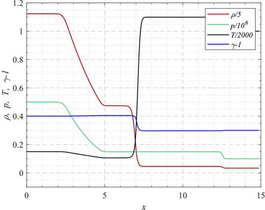
Figure 6: Quantity profiles of 1-D Sod problem solved by the hybrid fluxes.

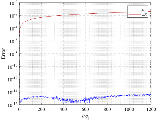
Figure 7: Conservation loss of mass and total energy in 1-D Sod problem solved by hybrid fluxes.

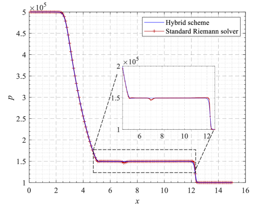
(a)

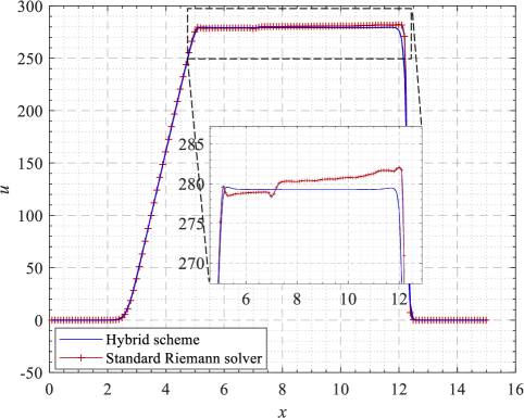
(b)

Figure 8: Comparison of the 1-D (a) pressure and (b) velocity profiles of the 1-D Sod problem solved by the hybrid scheme and the conservative Riemann solver.

4.3.2 2-D inert shock-bubble interaction

To further valid the hybrid solver in handling multi-dimensional viscous problems, a 2-D inert shock-bubble interaction example was simulated by solving the viscous Navier-Stokes equations. This example involves the passage of an air shock wave through a helium bubble suspended in the medium, as depicted in Fig. Scenario of a helium bubble deformed by a normal shock. Three time-dependent characteristic points are labelled respectively as the ”upstream”, ”downstream” and ”jet” points.. In the past, this example has frequently served as a benchmark for two-dimensional simulation validations for interface-capturing methods [46, 47, 7]. The computational configuration is a rectangular domain defined by $\Omega=\left[0,0.325\right]$ m $\times\left[0,0.0455\right]$ m. The simulation starts with a normal shock wave situated at $\bar{x}$ = 0.225 m, preceded by the placement of the helium bubble on its left side. A uniform grid of $\Delta x=\Delta y$ = 0.01 cm is employed.

It can be observed in Fig. Comparison of the bubble deformation process calculated by the hybrid and the conservative schemes. that the conventional conservative shock-capturing scheme introduces excessive spurious numerical oscillations when dealing with the interaction process between the shock and bubble, resulting in a visibly unstable structure of the helium plume, which should have been properly dissipated by the viscosity in the Navier-Stokes equations. In contrast, the hybrid scheme yields a significantly smoother bubble interface and effectively exhibits the diffusion effect. It is evident that the use of conservative scheme leads to a noticeable expansion in bubble volume over time, which can also be inferred from Fig. ‣ Trajectory of three characteristic points obtained with the (a) conservative flux and (b) hybrid fluxes, as compared to the results calculated by the front-tracking method of [47].. Here, the dotted markers represent the bubble trajectories calculated using a front-tracking method [47]. Clear discrepancies emerge between the predictions of the front-tracking method and the traditional conservative scheme concerning the ”upstream” and ”jet” points, exacerbated over time due to numerical oscillation errors. This amplification of differences suggests a numerical inflation of the bubble volume, highlighting a failure in accurate numerical prediction. Conversely, Figure ‣ Trajectory of three characteristic points obtained with the (a) conservative flux and (b) hybrid fluxes, as compared to the results calculated by the front-tracking method of [47]. illustrates that results obtained with the improved hybrid approach align more favorably with the one from the sharp-interface capturing method. This example also verifies that the multi-dimensional solution procedure of Algorithm Hybridization methodology works reliably.

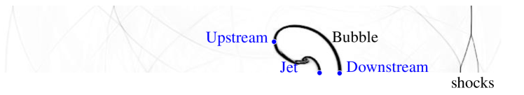
Figure 9: Scenario of a helium bubble deformed by a normal shock. Three time-dependent characteristic points are labelled respectively as the ”upstream”, ”downstream” and ”jet” points.

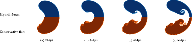
Figure 10: Comparison of the bubble deformation process calculated by the hybrid and the conservative schemes.

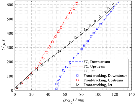
(a)

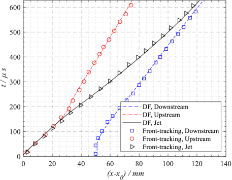
(b)

Figure 11: Trajectory of three characteristic points obtained with the (a) conservative flux and (b) hybrid fluxes, as compared to the results calculated by the front-tracking method of [47].

5 Chemically reactive problems

So far, we have constructed an efficient, accurate hybrid solver tailored especially for thermally perfect gases. It remains stable under shock capturing by the TVD limiting and the characteristic decomposition procedures and is capable of resolving material interfaces free of oscillations and with marginal conservation loss. The AMR technique is also employed to achieve efficient computations. Section Verification and validation demonstrated the preferable properties of the extended double-flux scheme. The hybridization methodology has been verified and validated in Section Verification and validation, and its combination with AMR will be presented to be working well in the subsequent Sections 2-D DDT (Deflagration-to-Detonation Transition) in a smooth channel. In the final section, an example of a complex planar RDE (Rotating Detonation Engine) with non-premixed gases will illustrate the superiority of the method developed in this paper.

5.1 1-D advection-diffusion of a reactive $\ce{H2}$ bubble in $\ce{O2}$ gases

In this example, the complete multicomponent Navier-Stokes equations with diffusion and chemistry terms are solved. We use this example to elucidate the failure of a fully conservative method as well as the capacity of the extended double-flux scheme in resolving a reactive contact discontinuity with minor pressure gradient.

The initial and physical boundary conditions are set up following Ref. [15], Section3.2. The initial profiles of $Y_{\mathrm{H}_{2}}$ and $T$ are

$$T =1500\left[1-\frac{1}{3}\tanh\left(C_{r}\left(\frac{l}{2}-\left|x-x_{0}\right|\right)\right)\right],$$ (42a)

$$Y_{\mathrm{H}_{2}} =\frac{1}{2}\left[1+\tanh\left(C_{r}\left(\frac{l}{2}-\left|x-x_{0}\right|\right)\right)\right],$$ (42b)

$$u_{0} =10m/s,\quad\quad\quad p_{0}=1\times 10^{5},$$ (42c)

where the centre of the plateau $x_{0}$ = 1 cm, the length of the plateau $l$ = 6 mm and the parameter $C_{r}$ = 80. Burke’s reaction mechanism [37] is employed as the chemical kinetics.

As shown in Fig. ‣ 1-D reactive convection of hydrogen bubble solved with (a) extended double-flux scheme at $t_{1}$ = 0.1 ms and (b) fully conservative scheme at $t_{2}$ = 0.008 ms., the extended double-flux scheme produces smooth profiles of the temperature $T$ as well as the mass fractions $Y_{\ce{H2}}$ and $Y_{\ce{O2}}$ until to the time $t_{1}$. Although affected by the reaction process, the pressure exhibits negligible gradient at the reaction layers, possibly due to the dissipation of physical diffusion. By contrast, as in Fig. ‣ 1-D reactive convection of hydrogen bubble solved with (a) extended double-flux scheme at $t_{1}$ = 0.1 ms and (b) fully conservative scheme at $t_{2}$ = 0.008 ms., the pressure at the bubble fronts oscillates significantly upon initiation of the calculation when using a fully conservative scheme, which results in the asymmetry of the temperature spikes and the oscillations nearby. This kind of temperature oscillations at the material fronts might lead to a flawed description of the reaction process. According to our results, with the same calculation time, the averaged values of the temperature spikes obtained with the extended double-flux scheme and the fully conservative scheme at $t=t_{1}$ are respectively 330.6 K and 347 K, which is 4.96$\%$ variation.

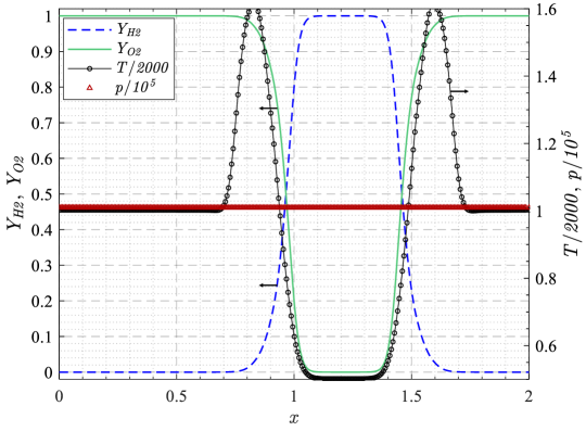
(a)

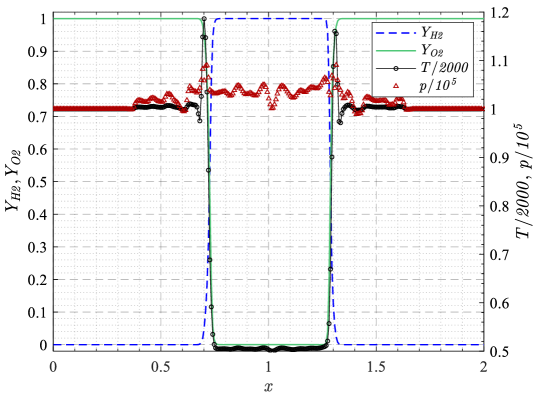
(b)

Figure 12: 1-D reactive convection of hydrogen bubble solved with (a) extended double-flux scheme at $t_{1}$ = 0.1 ms and (b) fully conservative scheme at $t_{2}$ = 0.008 ms.

5.2 2-D DDT (Deflagration-to-Detonation Transition) in a smooth channel

This example illustrates the capability of the new hybrid solver in handling premixed combustion phenomena efficiently and accurately, in the presence of strong shocks. The calculation domain is a rectangle of length 20 cm by 2 cm, with 400$\times$40 cells in the $x$- and $y$-direction. The case is initiated with quiescent, homogeneous $\ce{H2}$-$\ce{O2}$ premixed gas in the stoichiometric equivalent ratio, characterized with a Lewis number of $Le_{\text{eff}}$ = 0.8. Table Input parameters and output thermal properties for hydrogen-oxygen mixture at the equivalent ratio. $\delta_{\text{T}}=(T_{\text{ad}}-T_{0})/|\text{d}T/\text{d}x|_{\text{max}}$. lists the input parameters as well as the resulting flame properties obtained from Cantera [48].

Table 4: Input parameters and output thermal properties for hydrogen-oxygen mixture at the equivalent ratio. $\delta_{\text{T}}=(T_{\text{ad}}-T_{0})/|\text{d}T/\text{d}x|_{\text{max}}$.

Inputs Parameters
$p_{0}$	0.1 MPa	Initial pressure
$T_{0}$	300 K	Initial temperature
$\gamma$	1.4	Specific heat ratio
$\mu_{0}$	7.61e-05 kg/(m$\cdot$s)	Mixture-averaged viscosity
$\lambda_{0}$	1.875e-03 m2/s	Thermal diffusivity
Flame Properties
$Le_{\text{eff}}$	0.8	Effective Lewis number
$\delta_{T}$	2.59e-04 m	Laminar flame thickness
$S_{L}$	9.41 m/s	Laminar flame speed
$T_{\text{ad}}$	3071 K	Adiabatic flame temperature
$\Theta$	10.24	Thermal expansion ratio

The mixture is ignited initially at the end wall with an ignition radius of $r$ = 0.1 cm, and then the flame propagates from the closed end to the open end in an increasing speed due to the well-known thermal-shock interaction [49]. All boundaries except for the right one are set as no-slip solid walls while the right boundary is treated as an extrapolation outlet.

We simulate two cases with 3 and 4 refinement levels respectively, as listed in Table Refinement configuration of case 1 and case 2 in the premixed DDT example..

Table 5: Refinement configuration of case 1 and case 2 in the premixed DDT example.

	case 1	case 2
refinement levels $l$	3	4
refinement ratio $r$	(2,4)	(2,2,4)
minimum grid size $\delta_{min}$	62.5 $\mu m$	31.25 $\mu m$

Results obtained with the 3-level refinement are shown in Fig. Illustration of numerical flame acceleration and detonation initiation process with 3-level refinement (2,4) in case 1 by (a) shock-discontinuity flagging, (b) temperature and (c) refinement level diagrams.. The snapshots of the shock flagging criteria as well as the temperature diagrams during the dynamic DDT process illustrate that the hybridization described in Section Hybridization methodology worked quite well, identifying most of the important discontinuous phenomena such as the compression waves, the precursor shock as well as the detonation wave. To further assess the efficiency of the presented new hybrid solver in handling higher grid-level refinement, which is usually required for high resolution DDT simulation, we continue investigating the same configuration with a finer grid of a 4-level refinement.

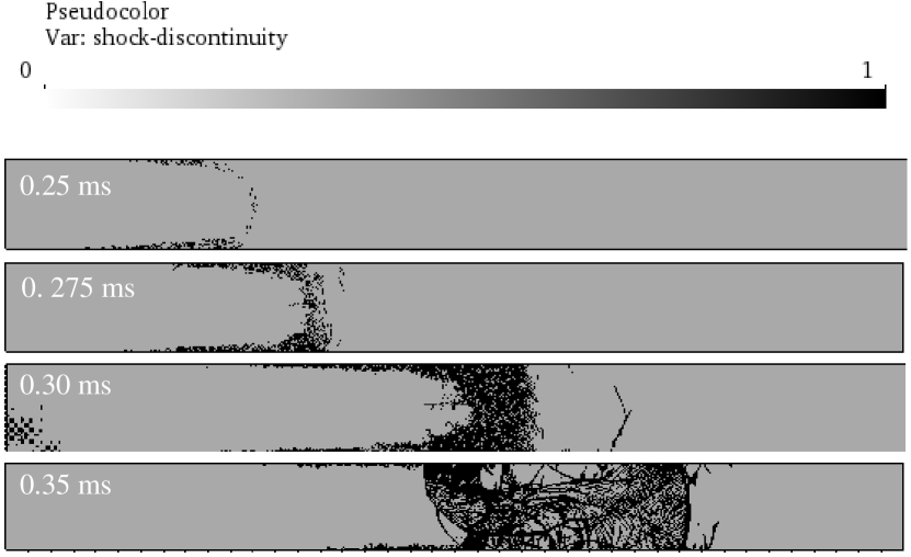
(a) shock-discontinuity flagging

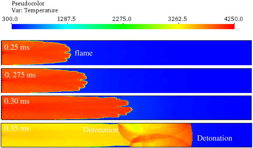
(b) temperature

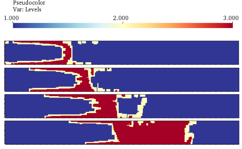
(c) refinement level

Figure 13: Illustration of numerical flame acceleration and detonation initiation process with 3-level refinement (2,4) in case 1 by (a) shock-discontinuity flagging, (b) temperature and (c) refinement level diagrams.

Figure Unstable cellular structures solved respectively by the fully conservative scheme and the hybrid scheme with 4-level refinement. illustrates the fine structures of an unstable flame front, obtained from the fully conservative and hybrid schemes with 4-level refinement respectively. As can be observed in Fig. Unstable cellular structures solved respectively by the fully conservative scheme and the hybrid scheme with 4-level refinement.(a), the flame front solved with the fully conservative scheme evolves into a single-cusp structure with a cell size approximately equal to $h$. In contrast, a multi-head cellular structure is established at the flame front in Fig. Unstable cellular structures solved respectively by the fully conservative scheme and the hybrid scheme with 4-level refinement.(b) solved by the hybrid solver, which aligns more with the most unstable wavelength $\lambda_{m}$ = 6$\delta_{T}$ as predicted by linear flame instability analysis [50, 51]. The length of $\lambda_{m}$ is also labelled in Fig. Unstable cellular structures solved respectively by the fully conservative scheme and the hybrid scheme with 4-level refinement. for comparison. We analyze this difference to be attributed to the transverse propagation of the spurious oscillation waves in Fig. Unstable cellular structures solved respectively by the fully conservative scheme and the hybrid scheme with 4-level refinement.(a), which causes the numerical merging of adjacent small cusps. For the hybrid counterparts, on the other hand, the material interfaces remain free of oscillation and thus reproduce the real-world flame evolution better.

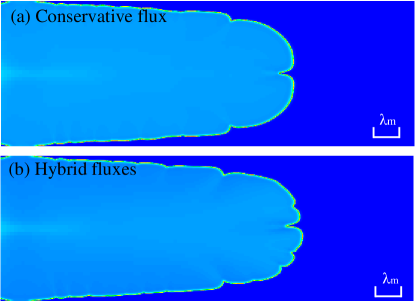
Figure 14: Unstable cellular structures solved respectively by the fully conservative scheme and the hybrid scheme with 4-level refinement.

In general, Figs Comparison of time-space flame front trajectories obtained using the fully conservative scheme and extended double-flux scheme with SAMR, as well as the one obtained using a uniform fine grid. and Comparison of the end-wall pressure history obtained using the fully conservative scheme and the hybrid scheme with SAMR. both illustrate that the usage of the double-flux method generates a more accelerated flame as compared to the one solved with the conventional scheme. That is reasonable because a sharper folding flame profile obtained means more heat release onto the leading shock that will compress the reactants behind the flame. This is also evidenced by the early agreement of the two curves in Figs. Comparison of time-space flame front trajectories obtained using the fully conservative scheme and extended double-flux scheme with SAMR, as well as the one obtained using a uniform fine grid. and Comparison of the end-wall pressure history obtained using the fully conservative scheme and the hybrid scheme with SAMR. during which the separate two flames are more dominated by initial thermal expansion instead of flame instabilities. In Fig. Comparison of time-space flame front trajectories obtained using the fully conservative scheme and extended double-flux scheme with SAMR, as well as the one obtained using a uniform fine grid., we also compare the result solved by a uniform grid with the grid size $\delta_{u}$ = 31.25 $\mu m$, which corresponds right to the finest grid size $\delta_{min}$ in the 4-level SAMR configuration. Generally, the result is in agreement with the one solved by the SAMR, illustrating the SAMR working well. Table Comparison of the wall cpu time calculated by a 4-level SAMR grid and a uniform grid with the grid size corresponding to the finest one in the 4-level SAMR grid. compares the total wall cpu time for a run on 400 cores, which proves again the efficiency of our presented hybrid method as well as the methodology by combining the hybrid solver with the SAMR technique.

Table 6: Comparison of the wall cpu time calculated by a 4-level SAMR grid and a uniform grid with the grid size corresponding to the finest one in the 4-level SAMR grid.

	SAMR Grids,		Uniform Grids
	4-level refinement (2,2,4)
	conservative scheme	hybrid scheme	hybrid scheme
wall cpu time [s]	10429.475	10920.522	27393.394

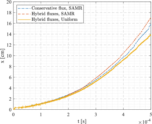
Figure 15: Comparison of time-space flame front trajectories obtained using the fully conservative scheme and extended double-flux scheme with SAMR, as well as the one obtained using a uniform fine grid.

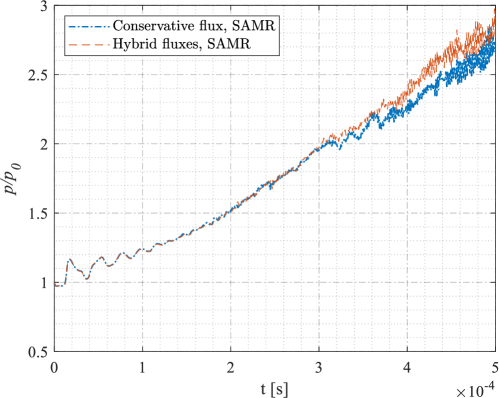
Figure 16: Comparison of the end-wall pressure history obtained using the fully conservative scheme and the hybrid scheme with SAMR.

5.3 2-D non-premixed planar RDE (Rotating Detonation Engine)

In this section, a detonation wave flowing over $\ce{H2}$/air slots on a planar wall, i.e., a 2D non-premixed planar RDE configuration, is simulated. The computational domain is a rectangle with $n_{x}\times n_{y}$ = 100 $\times$ 400 cells in the $x$- and $y$-direction. The domain lengths in the $x$- and $y$-directions are $l_{x}$=5 cm and $l_{y}$=20 cm, respectively.

As for the boundary conditions, both of the upper and lower ends of this computational domain are treated as periodic. At the left end, a total of $N$=40 injection nozzles are distributed uniformly along the length at an interval of $d_{1}$=3 mm with non-premixed $\ce{H2}$ and air injected separately in their sonic speeds. The width of each slot is $d_{2}$=2 mm. In this non-premixed scenario, the injection width of $\ce{H2}$ is 1/4 of the whole slot width and so the air fills the remaining 3/4 part in each slot. During each interval, a slip wall condition is used. In this example, the injection time depends on the relation of the total pressure of the non-premixed gases $p_{\text{tol}}$ and the dynamic interior pressure $p_{\text{in}}$ due to wave propagation. When $p_{\text{tol}}\geq p_{\text{in}}$, the injection is initiated, otherwise the slots are treated numerically as slip walls. The injection total pressure and temperature are set to $p_{\text{tol}}$ = 0.5 MPa and $T_{\text{tol}}$ = 300 K, respectively. At the right end of the domain, a hybrid subsonic/supersonic outflow boundary is applied.

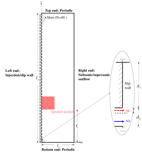
Figure 17: Numerical configuration of the 2-D planar RDE example.

This example is initiated by placing an ignition hot pocket onto the reactive mixtures, as depicted in Fig. Numerical configuration of the 2-D planar RDE example.. Owing to the use of periodic boundary condition, the detonation propagates periodically within the computational domain. The total simulation time is 2 ms, during which the detonation cycle occurs about 21 times. It can be observed from Fig. Pressure time history at line x = 1 cm solved by the conservative and hybrid schemes. that except from the first detonation cycle, divergence of the detonation propagation trajectories solved by the fully conservative and hybrid schemes is continuously increasing. The first detonation cycle, on the other hand, remains unaffected mainly due to the imposition of the initial condition during which the injection and mixing processes have had no effects yet.

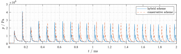
Figure 18: Pressure time history at line x = 1 cm solved by the conservative and hybrid schemes.

To illustrate this divergence, the beginning stage of the second detonation cycle is shown in Fig. Comparison of dynamic injection and detonation wave propagation calculated by the conservative and hybrid schemes. Left column: conservative scheme; Middle column: hybrid scheme; Right column: shock flagging., which depicts a typical temperature and shock flagging fields during this stage. In the simulation result from the conservative scheme, a partial extinction phenomenon can be seen clearly in Figs. $t$ = 0.1625 ms to $t$ = 0.1825 ms that occurs far from the injection slots and where the detonation front merges with the previous burned products . As the detonation wave travels further, the extinction becomes more severe. On the other hand, the simulation result from the new hybrid scheme shows clearly that the detonation wave as well as the detached compression waves behind it are well-flagged with the shock sensor presented in Section Hybridization methodology. Meanwhile, in contrast with the result obtained from the conservative scheme, it can also be observed that the head of the reaction wave is continuously coupled with the precursor shock, or else, the detonation is self-sustained during its propagation.

To uncover the underlying mechanism of such a significant divergence, we analyze the mixing fields derived respectively from the conservative and presented hybrid schemes, represented by the mass fraction of $\ce{H2}$ in Fig. mass fraction of H2 fields. It can be observed that the mixing region solved with the conservative scheme is much more oscillatory than that solved with the presented hybrid scheme. This kind of spurious oscillation interrupts the regular injection mixing process, and thus pollutes the mixing regions. By taking the $x$-axis direction as the reference direction, this interaction between the transverse oscillation waves and the longitudinal injection mixing would cause such a huge mixing flaw, especially in such a device with multiple injection slots and multiple injection mixing occurring simultaneously.

To take a deeper look at this phenomena from Fig. local ER fields, we could finally conclude that the partial detonation extinction essentially originates from its local high equivalence ratio (ER). The presented hybrid solver performs better to resolve the injection mixing process and thus derives a more suitable low-ER mixing region for detonation sustainability. Therefore, we can conclude that when the traditional conservative scheme is utilized on a non-premixed combustion scenario, the resulting impact is can be quite catastrophic, which fortunately can be cured by using the hybrid scheme presented in this paper.

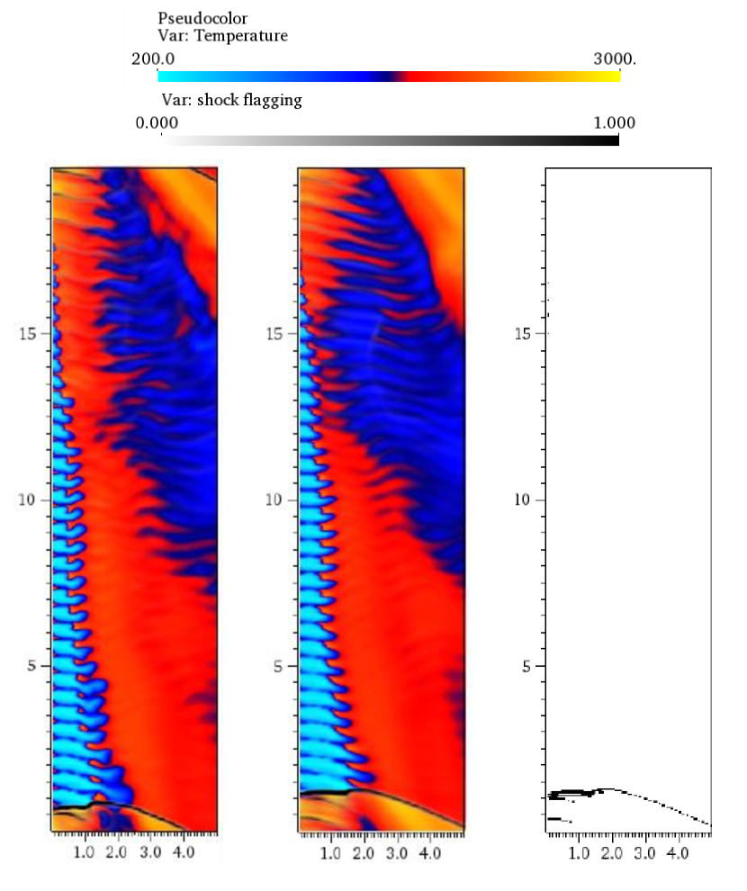
(a) $t$ = 0.1625 ms

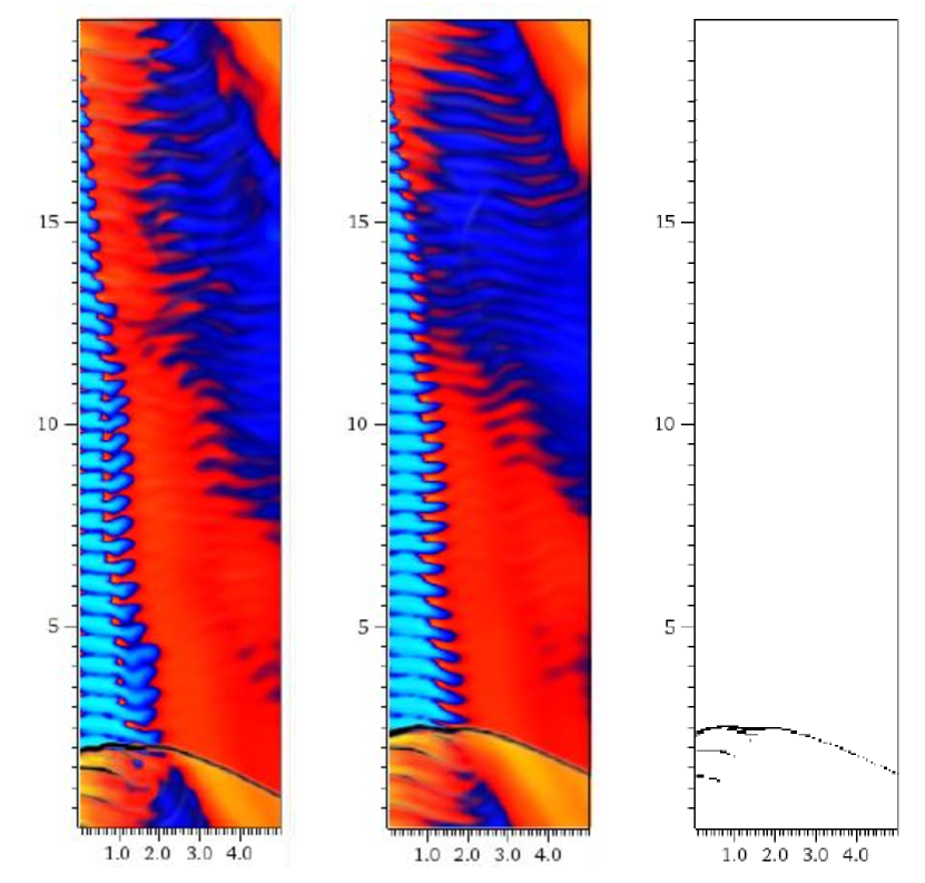
(b) $t$ = 0.1692 ms

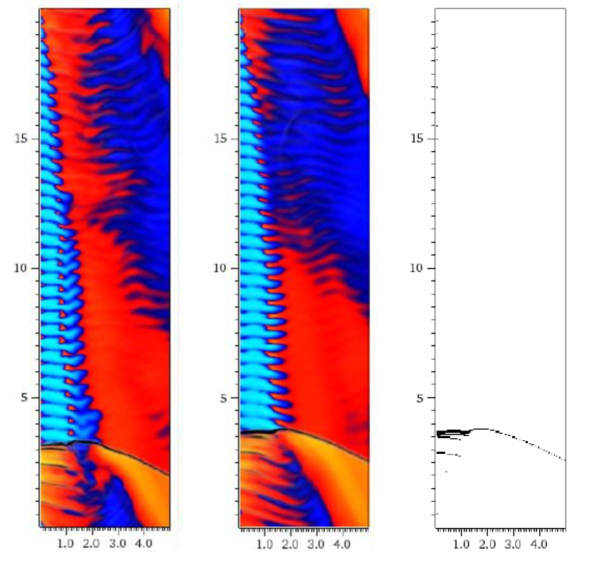
(c) $t$ = 0.1758 ms

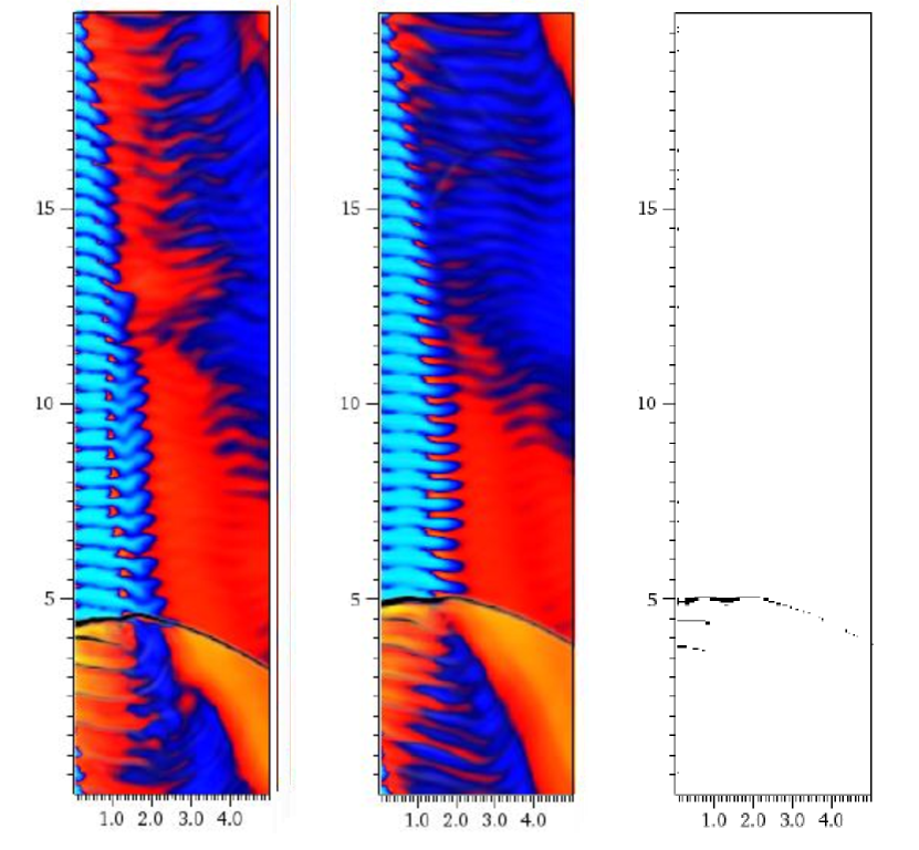
(d) $t$ = 0.1825 ms

Figure 19: Comparison of dynamic injection and detonation wave propagation calculated by the conservative and hybrid schemes. Left column: conservative scheme; Middle column: hybrid scheme; Right column: shock flagging.

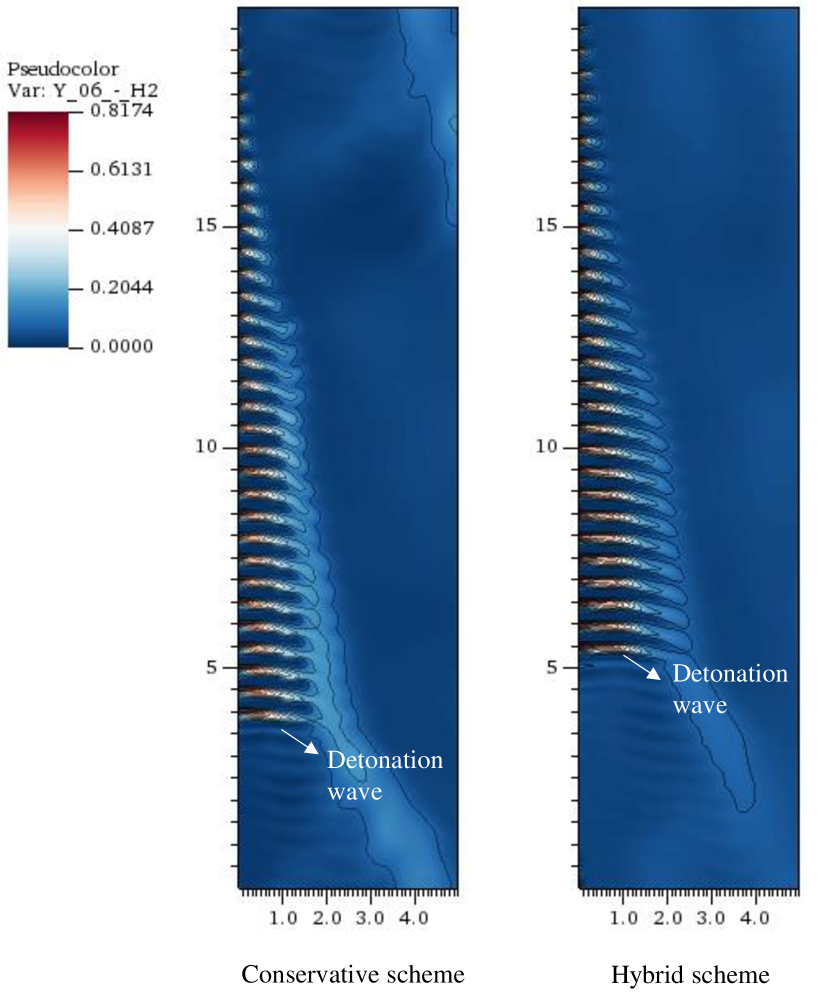
(a) mass fraction of H2 fields

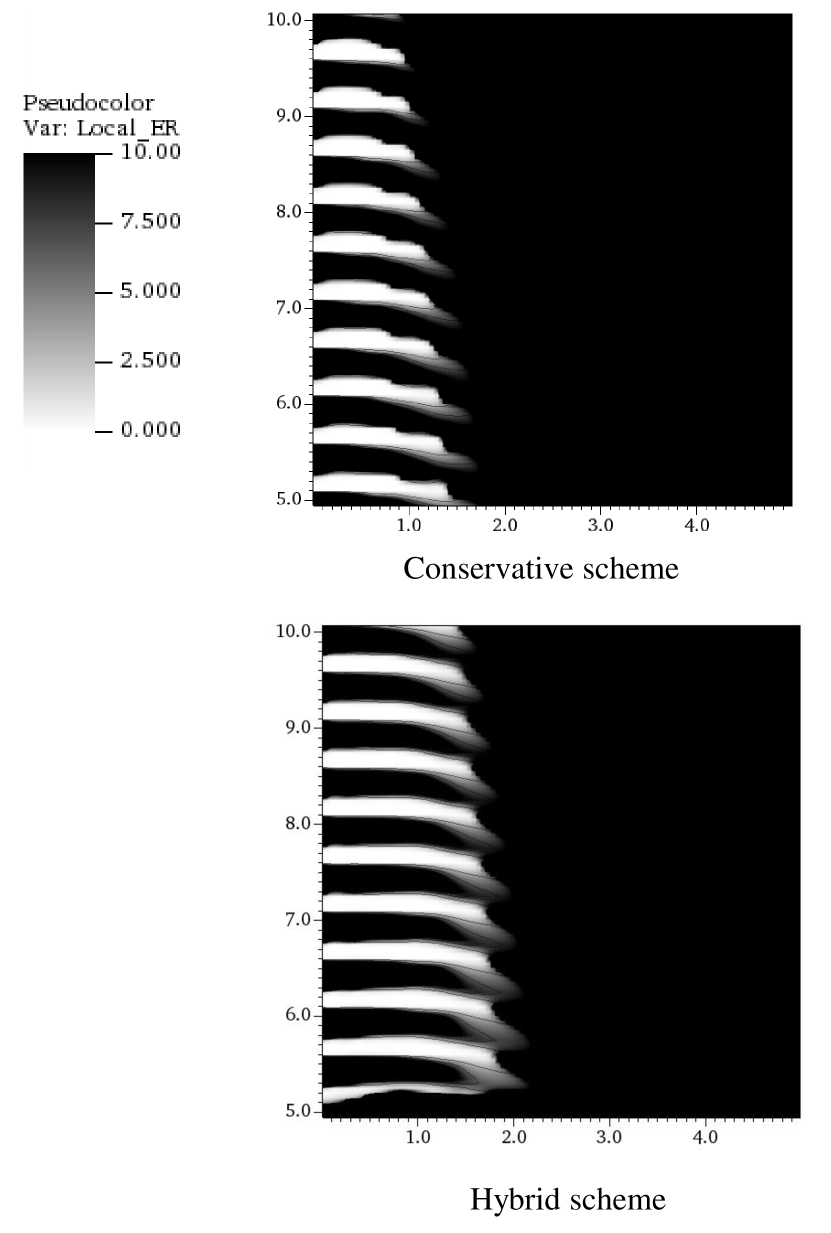
(b) local ER fields

Figure 20: Comparison of the (a) mass fraction of H2 global fields, (b) local equivalence ratio (ER) local fields calculated by the conservative and hybrid schemes.

6 Conclusion

The present study has successfully advanced a hybrid methodology within the finite-volume method, achieving a verified precision of second-order accuracy. The proposed new hybrid solver merges an extended double-flux strategy with conventional conservative methodologies, thereby ensuring enhanced stability and accuracy in multi-dimensional scenarios.

Central to this solver are the carefully tailored hybrid schemes for managing convective fluxes and interpolations. These designs guarantee optimal performance in maintaining solution stability while simultaneously delivering high-fidelity results, even under challenging conditions that combine material interfaces with shock discontinuities.

To extend the original double-flux technique, this paper put forth two full computational approaches, which have both proven reliable and efficient in suppressing pressure oscillations occurring at the material interfaces and at the same time require only one auxillary variable $\hat{\gamma}$, with tiny difference in momentum conservation preservation.

Extensive validations have conclusively demonstrated the efficiency and resilience of our solver in tackling multi-dimensional, shock-interface challenges, even in scenarios complicated by viscosity and chemical reactions by combining with the adaptive mesh refinement (AMR) technique. In the future, we expect to leverage the solver to handle large-scale compressible chemically reacting problems.

Appendix A Hybridized solution procedure

Algorithm 1 Hybridization methodology

1:  Calculate and store cell-based auxiliary variable $\hat{\gamma}$ using either Eq. Approach A or Eq. Approach B.

2:  Compute the troubled-cell indicator $S_{k}$ for shock detection ($>S_{k}^{T}$ using shock-capturing scheme, $>S_{k}^{T}$ with extended double-flux scheme).

3:  if $S_{k}<S_{k}^{T}$ then

4:     Save $\boldsymbol{U^{n}}$ first

5:     First RK Stage:

6:     Interpolate primitive variables onto cell edges; calculate inconsistent numerical fluxes using the extended double-flux scheme with the addition of viscous fluxes

7:     Update state vector $\boldsymbol{U^{n}}$ with dual edge fluxes to obtain $\boldsymbol{U^{*}}$.

8:     Update primitive variables as follows:

9:         $Y_{i}^{*}=\frac{(\rho Y_{i})^{*}}{\sum(\rho Y_{i})^{*}}$, $u^{*}=\frac{(\rho u)^{*}}{\sum(\rho Y_{i})^{*}}$, $v^{*}=\frac{(\rho v)^{*}}{\sum(\rho Y_{i})^{*}}$

10:         $p^{*}=\left(\hat{\gamma}-1\right)\left((\rho E)^{*}-(\rho h_{0}^{f})^{*}-\frac{\rho^{*}\boldsymbol{u}^{*2}}{2}\right)$, $T^{*}=\frac{p^{*}}{RU\sum\frac{(\rho Y_{i})^{*}}{W_{i}}}$

11:     Second RK Stage:

12:     Repeat steps 6-10 for updating of state vector $\boldsymbol{U^{*}}$ to get the final state $\boldsymbol{U^{n+1}}$.

13:     Update thermodynamic variables:

14:         $(C_{pi}^{*})^{n+1}=C_{pi}^{*}(T^{n+1})$, $(\hat{\gamma})^{n+1}=\frac{C_{p}^{*}}{C_{p}^{*}-R}$

15:     Correct the total energy $(\rho E)^{n+1}$:

16:         $(\rho E)^{n+1}=\frac{p^{n+1}}{(\hat{\gamma})^{n+1}-1}+(\rho h_{0}^{f})^{n+1}+\frac{(\rho\boldsymbol{u}^{2})^{n+1}}{2}$

17:  else

18:     Save $\boldsymbol{U^{n}}$ first

19:     First RK Stage:

20:     Interpolate charatertistic variables onto cell edges; calculate conservative numerical fluxes using the conservative scheme with the addition of viscous fluxes

21:     Update state vector $\boldsymbol{U^{n}}$ with single edge flux to obtain $\boldsymbol{U^{*}}$.

22:     Second RK Stage:

23:     Repeat steps 20-21 for updating of $\boldsymbol{U^{*}}$ to get the final state $\boldsymbol{U^{n+1}}$.

24:  end if

Appendix B Left and right characteristic matrix of multicomponent Navier-Stokes equations

The Jacobian matrix $\mathrm{A}_{1}(\mathrm{q})$ has a complete set of eigenvectors, hence it is diagonalizable with $\mathbf{R}_{1}^{-1}(\mathbf{q})\mathbf{A}_{1}(\mathbf{q})\mathbf{R}_{1}(\mathbf{q})=\boldsymbol{\Lambda}_{1}(\mathbf{q})$ for all admissible states $\mathbf{q}$ with $\boldsymbol{\Lambda}_{1}(\mathbf{q})=\operatorname{diag}\left(u_{1}-c,u_{1},\ldots,u_{1},u_{1}+c\right)$. In the matrix of right eigenvectors

$$\mathbf{R}_{1}(\mathbf{q}) =\left[\begin{array}[]{cccccccc}Y_{1}&1&0&\ldots&0&0&0&Y_{1}\\ \vdots&0&&\ddots&\vdots&\vdots&\vdots&\vdots\\ Y_{K}&0&\ldots&0&1&0&0&Y_{K}\\ u_{1}-c&u_{1}&\ldots&u_{1}&0&0&u_{1}+c\\ u_{2}&u_{2}&\ldots&u_{2}&1&0&u_{2}\\ u_{3}&u_{3}&\ldots&u_{3}&0&1&u_{3}\\ H-u_{1}c&\mathbf{u}^{2}-\frac{\phi_{1}}{\bar{\gamma}}&\ldots&\mathbf{u}^{2}-\frac{\phi_{K}}{\bar{\gamma}}&u_{2}&u_{3}&H+u_{1}c\end{array}\right]$$ (50)

the first and the last column are the vectors that span up the one-dimensional vector spaces corresponding to $\textit{u}_{1}-\textit{c}$ and $\textit{u}_{1}+\textit{c}$. The vectors of the columns 2 to K+3 span up the K+2-dimensional vector space for $\textit{u}_{1}$. $\textbf{R}1(\textbf{q})$ has full rank and is therefore inversible for all admissible states. The left eigenvector matrix reads

$$\mathbf{L}_{1}(\mathbf{q}) =\frac{1}{c^{2}}\left[\begin{array}[]{ccccccccc}\frac{\phi_{1}+u_{1}c}{2}&&&\ldots&\frac{\phi_{K}+u_{1}c}{2}&-\frac{\bar{\gamma}u_{1}+c}{2}&-\frac{\bar{\gamma}}{2}u_{2}&-\frac{\bar{\gamma}}{2}u_{3}&\bar{\gamma}\\ c^{2}-Y_{1}\phi_{1}&-Y_{1}\phi_{2}&&\ldots&-Y_{1}\phi_{K}&Y_{1}\bar{\gamma}u_{1}&Y_{1}\bar{\gamma}u_{2}&Y_{1}\bar{\gamma}u_{3}&-Y_{1}\bar{\gamma}\\ -Y_{2}\phi_{1}&c^{2}-Y_{2}\phi_{2}&\ldots&-Y_{2}\phi_{K}&&&&\\ \vdots&&\ddots&&\vdots&\vdots&\vdots&\vdots&\vdots\\ -Y_{K-1}\phi_{1}&\ldots&c^{2}-Y_{K-1}\phi_{K-1}&-Y_{K-1}\phi_{K}&&&&\\ -Y_{K}\phi_{1}&\ldots&-Y_{K}\phi_{K-1}&c^{2}-Y_{K}\phi_{K}&Y_{K}\bar{\gamma}u_{1}&Y_{K}\bar{\gamma}u_{2}&Y_{K}\bar{\gamma}u_{3}&-Y_{K}\bar{\gamma}\\ -u_{2}c^{2}&&\ldots&-u_{2}c^{2}&0&c^{2}&0&0\\ -u_{3}c^{2}&&\ldots&-u_{3}c^{2}&0&0&c^{2}&0\\ \frac{\phi_{1}-u_{1}c}{2}&&\ldots&\frac{\phi_{K}-u_{1}c}{2}&-\frac{\bar{\gamma}u_{1}-c}{2}&-\frac{\bar{\gamma}}{2}u_{2}&-\frac{\bar{\gamma}}{2}u_{3}&\bar{\gamma}\end{array}\right]$$ (60)

with

$$\phi_{i}:=\frac{\partial p}{\partial\rho_{i}}=\frac{R}{R-c_{p}}\left(h_{i}-\frac{\mathbf{u}^{2}}{2}\right)-\frac{c_{p}}{R-c_{p}}R_{i}T=\bar{\gamma}\left(\frac{\mathbf{u}^{2}}{2}-h_{i}\right)+\gamma R_{i}T,\quad\hat{\gamma}=\gamma-1.$$ (61)

Appendix C Procedures for characteristic decomposition applied to the MUSCL reconstruction

The characteristic decomposition procedures applied here are those proposed in [52], only with a small modification. First, the characteristic variables at cell $j$ are obtained with conservative variables approximated onto the characteristic space by

$$\boldsymbol{W}_{j}=\boldsymbol{L}_{i}\boldsymbol{Q}_{j},\quad j=i-1,i,i+1.$$ (62)

Then the slope of characteristic variables at cell $i$ is given by

$$\Delta\boldsymbol{W}_{i} =\Phi\left(\Delta\boldsymbol{W}_{i-1/2},\Delta\boldsymbol{W}_{i+1/2}\right),$$ (63)

where $\Phi$ represents the slope limiter, with $\Delta\boldsymbol{W}_{i+1/2}=\boldsymbol{W}_{i+1}-\boldsymbol{W}_{i}$.

The slope obtained in each characteristic field can then be projected back to the component space by

$$\Delta\boldsymbol{Q}_{i}=\boldsymbol{R}_{i}\Delta W_{i}.$$ (64)

Finally, the left and right values at the interface can be acquired by

$$\boldsymbol{Q}_{i+1/2}^{L}=\boldsymbol{Q}^{l}_{i}+\frac{1}{2}\Delta\boldsymbol{Q}_{i},$$ (65)

$$\boldsymbol{Q}_{i-1/2}^{R}=\boldsymbol{Q}^{l}_{i}-\frac{1}{2}\Delta\boldsymbol{Q}_{i}.$$ (66)

Here, $L_{i}$ and $R_{i}$ are the left and right eigenvector matrices of the Jacobian matrix $A_{i}$. This MUSCL scheme is able to maintain good robustness behind the shock discontinuity with relatively low computational cost.

References

- [1] B. Larrouturou, How to preserve the mass fractions positivity when computing compressible multi-component flows, Journal of computational physics 95 (1) (1991) 59–84.
- [2] S. Karni, Multicomponent flow calculations by a consistent primitive algorithm, Journal of Computational Physics 112 (1) (1994) 31–43.
- [3] R. Abgrall, How to prevent pressure oscillations in multicomponent flow calculations: a quasi conservative approach, Journal of Computational Physics 125 (1) (1996) 150–160.
- [4] V. T. Ton, Improved shock-capturing methods for multicomponent and reacting flows, Journal of Computational Physics 128 (1) (1996) 237–253.
- [5] P. Jenny, B. Müller, H. Thomann, Correction of conservative euler solvers for gas mixtures, Journal of Computational Physics 132 (1) (1997) 91–107.
- [6] K.-M. Shyue, An efficient shock-capturing algorithm for compressible multicomponent problems, Journal of Computational Physics 142 (1) (1998) 208–242.
- [7] R. F. Johnson, A. D. Kercher, A conservative discontinuous galerkin discretization for the chemically reacting navier-stokes equations, Journal of Computational Physics 423 (2020) 109826.
- [8] R. P. Fedkiw, B. Merriman, S. Osher, High accuracy numerical methods for thermally perfect gas flows with chemistry, Journal of Computational Physics 132 (2) (1997) 175–190.
- [9] R. P. Fedkiw, B. Merriman, S. Osher, Efficient characteristic projection in upwind difference schemes for hyperbolic systems: the complementary projection method, Journal of Computational Physics 141 (1) (1998) 22–36.
- [10] R. P. Fedkiw, T. Aslam, B. Merriman, S. Osher, A non-oscillatory eulerian approach to interfaces in multimaterial flows (the ghost fluid method), Journal of computational physics 152 (2) (1999) 457–492.
- [11] R. P. Fedkiw, Coupling an eulerian fluid calculation to a lagrangian solid calculation with the ghost fluid method, Journal of Computational Physics 175 (1) (2002) 200–224.
- [12] C.-H. Chang, X. Deng, T. G. Theofanous, Direct numerical simulation of interfacial instabilities: a consistent, conservative, all-speed, sharp-interface method, Journal of Computational Physics 242 (2013) 946–990.
- [13] J. Luo, X. Hu, N. A. Adams, A conservative sharp interface method for incompressible multiphase flows, Journal of Computational Physics 284 (2015) 547–565.
- [14] L. Xu, W. Yang, T. Liu, An interface treatment for two-material multi-species flows involving thermally perfect gases with chemical reactions, Journal of Computational Physics 448 (2022) 110707.
- [15] G. Billet, R. Abgrall, An adaptive shock-capturing algorithm for solving unsteady reactive flows, Computers & fluids 32 (10) (2003) 1473–1495.
- [16] R. W. Houim, K. K. Kuo, A low-dissipation and time-accurate method for compressible multi-component flow with variable specific heat ratios, Journal of Computational Physics 230 (23) (2011) 8527–8553.
- [17] Y. Lv, M. Ihme, Discontinuous galerkin method for multicomponent chemically reacting flows and combustion, Journal of Computational Physics 270 (2014) 105–137.
- [18] R. Abgrall, S. Karni, Computations of compressible multifluids, Journal of computational physics 169 (2) (2001) 594–623.
- [19] R. W. Houim, A. Ozgen, E. S. Oran, The role of spontaneous waves in the deflagration-to-detonation transition in submillimetre channels, Combustion Theory and Modelling 20 (6) (2016) 1068–1087.
- [20] G. Goodwin, R. Houim, E. Oran, Effect of decreasing blockage ratio on ddt in small channels with obstacles, Combustion and Flame 173 (2016) 16–26.
- [21] K. Bando, M. Sekachev, M. Ihme, Comparison of algorithms for simulating multi-component reacting flows using high-order discontinuous galerkin methods, in: AIAA Scitech 2020 Forum, 2020, p. 1751.
- [22] E. Johnsen, F. Ham, Preventing numerical errors generated by interface-capturing schemes in compressible multi-material flows, Journal of Computational Physics 231 (17) (2012) 5705–5717.
- [23] Y. Lv, M. Ihme, Development of discontinuous galerkin method for detonation and supersonic combustion, in: 51st AIAA Aerospace Sciences Meeting including the New Horizons Forum and Aerospace Exposition, 2013, p. 688.
- [24] J. Qiu, C.-W. Shu, A comparison of troubled-cell indicators for runge–kutta discontinuous galerkin methods using weighted essentially nonoscillatory limiters, SIAM Journal on Scientific Computing 27 (3) (2005) 995–1013.
- [25] L. Krivodonova, J. Xin, J.-F. Remacle, N. Chevaugeon, J. E. Flaherty, Shock detection and limiting with discontinuous galerkin methods for hyperbolic conservation laws, Applied Numerical Mathematics 48 (3-4) (2004) 323–338.
- [26] G. Li, J. Qiu, Hybrid weighted essentially non-oscillatory schemes with different indicators, Journal of Computational Physics 229 (21) (2010) 8105–8129.
- [27] D. J. Hill, D. I. Pullin, Hybrid tuned center-difference-weno method for large eddy simulations in the presence of strong shocks, Journal of Computational Physics 194 (2) (2004) 435–450.
- [28] J. L. Ziegler, R. Deiterding, J. E. Shepherd, D. I. Pullin, An adaptive high-order hybrid scheme for compressive, viscous flows with detailed chemistry, Journal of Computational Physics 230 (20) (2011) 7598–7630.
- [29] Z.-H. Jiang, C. Yan, J. Yu, Y. Li, Hybrid central-upwind finite volume schemes for solving the euler and navier–stokes equations, Computers & Mathematics with Applications 72 (9) (2016) 2241–2258.
- [30] S. Clain, S. Diot, R. Loubère, A high-order finite volume method for systems of conservation laws—multi-dimensional optimal order detection (mood), Journal of computational Physics 230 (10) (2011) 4028–4050.
- [31] R. Loubere, M. Dumbser, S. Diot, A new family of high order unstructured mood and ader finite volume schemes for multidimensional systems of hyperbolic conservation laws, Communications in Computational Physics 16 (3) (2014) 718–763.
- [32] M. Dumbser, O. Zanotti, R. Loubère, S. Diot, A posteriori subcell limiting of the discontinuous galerkin finite element method for hyperbolic conservation laws, Journal of Computational Physics 278 (2014) 47–75.
- [33] S. F. Davis, A simplified tvd finite difference scheme via artificial viscosity, SIAM journal on scientific and statistical computing 8 (1) (1987) 1–18.
- [34] C. R. Wilke, A viscosity equation for gas mixtures, The journal of chemical physics 18 (4) (1950) 517–519.
- [35] R. B. Bird, W. E. Stewart, E. N. Lightfoot, R. E. Meredith, Transport phenomena, Journal of The Electrochemical Society 108 (3) (1961) 78C.
- [36] S. Mathur, P. Tondon, S. Saxena, Thermal conductivity of binary, ternary and quaternary mixtures of rare gases, Molecular physics 12 (6) (1967) 569–579.
- [37] M. P. Burke, M. Chaos, Y. Ju, F. L. Dryer, S. J. Klippenstein, Comprehensive h2/o2 kinetic model for high-pressure combustion, International Journal of Chemical Kinetics 44 (7) (2012) 444–474.
- [38] E. F. Toro, Riemann solvers and numerical methods for fluid dynamics: a practical introduction, Springer Science & Business Media, 2013.
- [39] M.-S. Liou, A sequel to ausm: Ausm+, Journal of computational Physics 129 (2) (1996) 364–382.
- [40] P. Kaps, P. Rentrop, Generalized runge-kutta methods of order four with stepsize control for stiff ordinary differential equations, Numerische Mathematik 33 (1979) 55–68.
- [41] R. Deiterding, Parallel adaptive simulation of multi-dimensional detonation structures, Dissertation. de, 2003.
- [42] M. J. Berger, P. Colella, Local adaptive mesh refinement for shock hydrodynamics, Journal of computational Physics 82 (1) (1989) 64–84.
- [43] R. Deiterding, Block-structured adaptive mesh refinement-theory, implementation and application, in: Esaim: Proceedings, Vol. 34, EDP Sciences, 2011, pp. 97–150.
- [44] R. Deiterding, A parallel adaptive method for simulating shock-induced combustion with detailed chemical kinetics in complex domains, Computers & Structures 87 (11-12) (2009) 769–783.
- [45] X. Cai, J. Liang, R. Deiterding, Y. Mahmoudi, M. Sun, Experimental and numerical investigations on propagating modes of detonations: Detonation wave/boundary layer interaction, Combustion and flame 190 (2018) 201–215.
- [46] J. J. Quirk, S. Karni, On the dynamics of a shock–bubble interaction, Journal of Fluid Mechanics 318 (1996) 129–163.
- [47] H. Terashima, G. Tryggvason, A front-tracking/ghost-fluid method for fluid interfaces in compressible flows, Journal of Computational Physics 228 (11) (2009) 4012–4037.
- [48] D. G. Goodwin, R. L. Speth, H. K. Moffat, B. W. Weber, Cantera: An object-oriented software toolkit for chemical kinetics, thermodynamics, and transport processes, Zenodo (2018).
- [49] J. H. Lee, The detonation phenomenon, Cambridge University Press, 2008.
- [50] C. Altantzis, C. Frouzakis, A. Tomboulides, M. Matalon, K. Boulouchos, Hydrodynamic and thermodiffusive instability effects on the evolution of laminar planar lean premixed hydrogen flames, Journal of fluid mechanics 700 (2012) 329–361.
- [51] L. Berger, K. Kleinheinz, A. Attili, H. Pitsch, Characteristic patterns of thermodiffusively unstable premixed lean hydrogen flames, Proceedings of the Combustion Institute 37 (2) (2019) 1879–1886.
- [52] G.-S. Jiang, C.-W. Shu, Efficient implementation of weighted eno schemes, Journal of computational physics 126 (1) (1996) 202–228.