Scaling Laws for Online Advertisement Retrieval

Abstract.

The scaling law is a notable property of neural network models that researchers have discovered, which greatly propels the development of large language models. Scaling laws hold great promise in guiding model design and resource allocation. Recent research increasingly shows that scaling laws are not limited to NLP tasks or Transformer architectures; they also apply to domains such as recommendation, where there are scaling laws relating to the amount of training data, model size, and model performance metrics. However, there is still a lack of literature on scaling law research in industrial online advertisement retrieval systems. This may be because 1) identifying the scaling law for resource cost and online revenue is often expensive in both time and training resources for large-scale industrial applications, and 2) varying settings for different systems prevent the scaling law from being applied across various scenarios. To address these issues, we propose a lightweight paradigm to identify the scaling law of online revenue and machine cost for a certain online advertisement retrieval scenario with a low experimental cost. Specifically, we focus on a sole factor (FLOPs) and propose an offline metric named $R/R^{*}$ that exhibits a high linear correlation with online revenue for retrieval models. We estimate the machine cost offline via a simulation algorithm. Thus, we can transform most online experiments into low-cost offline experiments. We conduct comprehensive experiments to verify the effectiveness of our proposed metric $R/R^{*}$ and to identify the scaling law in the online advertisement retrieval system of Kuaishou. With the scaling law, we demonstrate practical applications for ROI-constrained model designing and multi-scenario resource allocation in the Kuaishou advertising system. To the best of our knowledge, this is the first work to study the scaling laws for online advertisement retrieval of real-world large-scale systems, showing great potential for scaling law in advertising system optimization.

1. Introduction

The neural scaling laws, describing how neural network performance changes with key factors (e.g. model size, dataset size, computational cost), have been discovered in various research areas (Kaplan et al., 2020; Hoffmann et al., 2022; Shin et al., 2023; Isik et al., 2024; Zhang et al., 2024a; Fang et al., 2024). Early research (Hestness et al., 2017) shows that the neural network performance is predictable when scaling training data size in various tasks such as neural machine translation and language modeling. Kaplan et al.((2020)) (Kaplan et al., 2020) further empirically verify the scaling law of Transformer architecture in language modeling, regarding the key factors (model size, data size, training cost) and training performance (PPL). Inspired by the scaling law, researchers extend the size of pre-trained language models and further empirically verify the scaling law by training GPT-3 (Brown, 2020). This wave of enthusiasm has led to the creation of GPT-3.5 and GPT-4 (Achiam et al., 2023), ushering in a new era of NLP research and applications.

Based on the scaling laws, the optimal key factors of the model can be determined under given constraints, thus guiding us in model design and resource allocation. Recommendation and advertising systems are mature commercial applications that prioritize ROI, making it highly valuable to explore whether there exists scaling laws for recommendation and advertising models. Due to the lack of a thriving community and open data ecosystem similar to NLP, research on model scaling is relatively scarce in the recommendation and advertisement areas. Early studies primarily gave some qualitative conclusions about model scaling (Shin et al., 2023; Zhang et al., 2024a). Fang et al.((2024)) (Fang et al., 2024) first attempt to give a quantitative scaling law of model performance and the amount of training data and model parameters based on public information retrieval benchmarks, and give the practice to solve the optimal amount of data and model parameters under a given total training resource.

However, there is still a lack of literature on scaling law research in real-world online recommendation and advertising systems. We attribute this to two main challenges: 1) For commercial systems, the scaling law should describe the relationship between business revenue and machine costs, rather than the relationship between computing volume, data volume, and offline metrics as seen in traditional research. Achieving this requires training numerous models and conducting extensive online experiments, which are prohibitively expensive in terms of time, manpower, and machine costs; and 2) varying settings across different systems prevent the scaling law from being universally applicable. As a result, to use scaling laws to guide system optimization in a specific scenario, one must first incur substantial costs to obtain the necessary parameters. This makes it impractical for commercial systems to identify and apply scaling laws in many real-world settings.

We aim to identify scaling laws in online advertising systems with low experimental costs and explore their applications in guiding system optimization. An advertising system typically consists of several subsystems, including the advertisement retrieval subsystem and the bidding and ranking subsystem. Each subsystem has its own technology stack, making it challenging to establish a unified paradigm for lightweight identification of scaling laws. In this work, we focus on the online advertisement retrieval subsystem, which selects the top-k ads for the next stage but does not determine the billing of ads. This subsystem is described in detail in Section 3.

To address the issue of high experimental costs, we propose a lightweight paradigm for identifying scaling laws in online advertisement retrieval. First, we introduce a novel offline metric, $R/R^{*}$, which incorporates the revenue information of each ad in the training data and exhibits a high linear correlation with online revenue for retrieval models. Note that we can obtain the specific relationship between $R/R^{*}$ and online revenue for our scenario through the records of daily iterations, theoretically eliminating the need for additional online experiments. Next, we conduct extensive offline experiments to verify the scaling behavior of MLP models in the retrieval scenario, where FLOPs serve as the independent variable and $R/R^{*}$ serves as the dependent variable. Our results show that these scaling behaviors follow a broken neural scaling law (Caballero et al., 2023). Finally, we propose a simple simulation algorithm, developed by our engineering team, to estimate the machine cost. By using the model size parameter as the decision variable and FLOPs and $R/R^{*}$ as intermediate variables, we can associate the model’s estimated machine cost with the estimated online revenue.

We conduct extensive online experiments to verify the effectiveness of our proposed $R/R^{*}$ metric. The results show that $R/R^{*}$ is a more advanced offline surrogate metric for online revenue compared to traditional metrics. When there is no revenue-related information recorded at the ad granularity in the training data, $NDCG$ can serve as a suitable substitute for $R/R^{*}$. Additionally, we demonstrate the applications of the scaling law in ROI-constrained model design and multi-scenario resource allocation. These applications result in a 0.85% and 2.8% improvement in online revenue, respectively, highlighting the significant value of the scaling law in guiding system optimization.

In general, our main contributions are three-fold: 1) We introduce an offline metric, $R/R^{*}$, which exhibits a strong linear correlation with online revenue, bringing significant convenience to the validation of scaling laws and the iterative development of retrieval models. 2) We provide a lightweight paradigm to identify the scaling laws between machine cost and online revenue and verify the existence of scaling laws in industrial advertisement retrieval scenarios. 3) We demonstrate practical applications of the scaling laws in the Kuaishou advertising system. With the scaling law of online revenue and machine cost, we can efficiently perform offline ROI estimations for hundreds of models with different sizes using just a few machines within a few days. The models obtained through this process have led to significant revenue improvement, highlighting the potential of scaling laws in optimizing advertising systems.

2. Related Work

2.1. Neural Scaling Laws

The neural scaling laws, widely recognized in Natural Language Processing and Computer Vision areas, establish predictable relationships between model performance and key factors such as model size, dataset size, computational cost, and post-training error rates. Hestness et al.((2017)) (Hestness et al., 2017) introduced a unified scaling law applicable to machine translation, image classification, and speech recognition, noting that different tasks exhibit distinct scaling coefficients. Kaplan et al.((2020)) (Kaplan et al., 2020) further elaborated on these laws, defining them through four parameters: model size (number of parameters), dataset size (number of tokens), computational cost (FLOPs), and training loss (perplexity per token). These relationships were empirically validated, including during the training of GPT-3 (Brown, 2020). Subsequently, Hoffmann et al.((2022)) (Hoffmann et al., 2022) presented the Chinchilla Scaling Law, which differs somewhat from (Kaplan et al., 2020) because of their different training setups. In addition to estimating the training loss of the model, Isik et al.((2024)) (Isik et al., 2024) further verified that there also exist scaling laws between the downstream task metrics and the model parameters. Caballero et al.((2023)) (Caballero et al., 2023) found that many scaling behaviors of artificial neural networks follow a smoothly broken power law (BNSL), verified on various NLP and CV tasks, covering a wide range of downstream tasks and model structures.

In the recommendation area, Shin et al.((2023)) (Shin et al., 2023) and Zhang et al.((2024a)) (Zhang et al., 2024a) conducted studies on whether there exist scaling laws for recommendation models and primarily provided qualitative conclusions. Fang et al.((2024)) (Fang et al., 2024) first proposed a quantitative scaling law in the recommendation area, which describes the relationship between the amount of training data, the size of model parameters, and an offline metric for query-document retrieval. Based on this scaling law, the optimal amount of data and model parameter allocation can be solved under a given total training resource. However, obtaining a multivariate scaling law requires a large number of experiments, and the offline metrics might not be a good indicator for online metrics, these make it somewhat difficult to apply in real-world industrial applications. In this paper, we focus on how to obtain the scaling law function between the model’s scalable hyper-parameters (such as the FLOPs) and the online revenue (the primary goal of the advertising system) with only a small amount of experimental cost.

2.2. Models and Evaluation for Online Advertisement Retrieval

Online advertising systems often adopt a cascade ranking framework (Qin et al., 2022; Wang et al., 2011; Gallagher et al., 2019; Chen et al., 2017). The cascade ranking usually includes two types of stages, namely retrieval and ranking. The retrieval stages take a set of terms as input and supply the top-k predicted terms to the next stage, which mainly focuses on order accuracy. The ranking stages in advertising systems should focus on not only the order accuracy but also the calibration accuracy (Huang et al., 2022; Sheng et al., 2023). These lead to some technique differences in retrieval and ranking stages, such as optimization objectives, surrogate losses, design of evaluation metrics, etc. In this work, we focus on the retrieval stages of online advertising systems.

The retrieval stages select the top-k set for the next stage, typically including multiple ranking pathways. In the retrieval stages, which normally refers to the ”Matching” or ”Pre-rank” stage in industrial systems, models often adopt a twin-tower (Covington et al., 2016) or MLP (Hornik et al., 1989) architecture. Some systems may also adopt more complex architectures like transformers (Vaswani et al., 2017). In terms of objective design, industrial systems usually aim to estimate CTR (He et al., 2014) and exposure probability of ads, and use learning-to-rank methods (Wang et al., 2018, 2024) to learn the results of ranking models. For evaluation of retrieval tasks, researchers commonly use OPA, NDCG, and Recall (Wang et al., 2024; Zangerle and Bauer, 2022; Bauer et al., 2024). However, existing metrics often have complex relationships with online revenue, thus we propose $R/R^{*}$, which exhibits a strong linear relationship with online revenue, to reduce the experimental cost of identifying the scaling law for industry scenarios.

3. Formulation of Online Advertisement Retrieval

3.1. Overview of Online Advertising System

Figure 1 illustrates a typical cascade ranking system for online advertisements deployed at Kuaishou Technology. This system is comprised of four main stages: Matching, Pre-ranking, Ranking, and Mix-ranking. The ”Matching” and ”Pre-ranking” stages serve as retrieval mechanisms, focusing on selecting candidate ads without directly impacting their billing. Conversely, the ”Ranking” stage plays a dual role by determining both the selection and billing of ads. It achieves this by predicting the eCPM (Effective Cost Per Mille) of each ad, serving as the standard for billing after its exposure. The ”Mix-ranking” stage integrates the outputs from the advertising and recommendation systems to decide the final set of items presented to the user. For advertising systems, the differences in the goal of the retrieval and ranking stages lead to some technical differences, such as training objectives, system design, evaluation metrics, etc. In this work, we focus on the scaling laws of retrieval stages.

Figure 2 shows the algorithm architecture of the Matching and Pre-ranking stages in the Kuaishou advertising system. They all adopt a multi-pathway ensemble architecture. The Matching stage can be divided into model-based pathways and rule-based pathways. The rule-based pathway can quickly filter out irrelevant ads using predefined criteria, ensuring compliance with regulations and improving ad relevance, while providing flexibility and transparency in the ad selection process. The model-based pathway uses machine learning algorithms to predict and select ads, achieving higher performance ceilings in ad selection. The Pre-ranking stage operates on the set of ads already selected by the Matching stage, and thus only employs the model-based pathways.

Model-based pathways in the Matching and Pre-ranking stages can typically be categorized based on different modeling objectives, such as revenue-oriented, user-interest-oriented, and lifetime value-oriented pathways. In advertising systems, revenue-oriented pathways usually carry the most weight. Since the earlier stages only need to perform set selection, Kuaishou’s advertising system employs Learning-to-Rank (LTR) methods to learn the optimal ranking order to maximize the revenue objective. The LTR pathway is the most prevalent and important in the system, as it is typically the primary focus for algorithm researchers to iterate and improve. Therefore, we use the Pre-ranking LTR pathway as a case study to verify scaling laws in online advertisement retrieval, which similarly applies to Matching models because they share the same multi-pathway architectures.

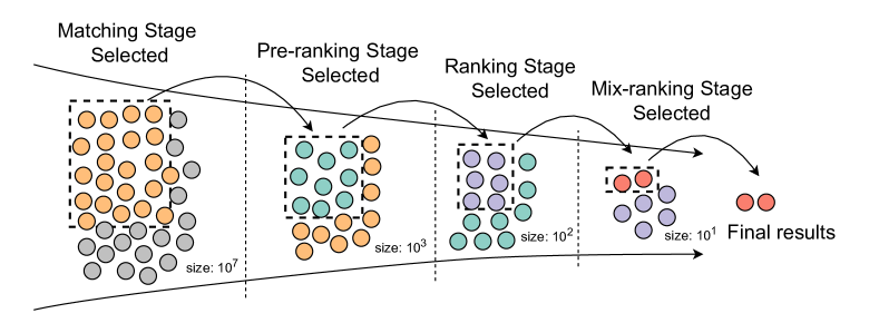
Figure 1. The cascade ranking architecture at Kuaishou Technology, includes four stages: Matching, Pre-ranking, Ranking, and Mix-ranking. Typically, we regard the ”Matching” and ”Pre-ranking” stages as retrieval stages, which do not decide the billing of ads.

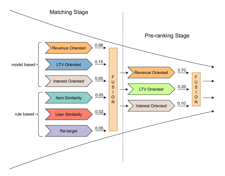
Figure 2. The multi-pathway architecture of Matching and Pre-ranking stages in Kuaishou advertising system. Each pathway has its own weight, which determines the proportion of ads sent to the next stage after the Fusion module.

3.2. Formulation of Retrieval Tasks

Here we give the formulation of retrieval tasks represented by learning-to-rank in the Pre-ranking stage. The organization of training samples and the surrogate loss follows the ARF (Wang et al., 2024). We randomly draw samples from the Pre-ranking, Ranking, and Mix-ranking stages. The training set can be formulated as:

(1) $$D_{train}=\{(f_{u_{i}},\{f_{a_{i}^{j}},v_{i}^{j},ecpm_{i}^{j}|1\leq j\leq n\})_{i}\}_{i=1}^{N}$$

where $u_{i}$ means the user of the $i$-th impression in the training set, $a^{j}$ means the $j$-th material for ranking in the system. $N$ is the number of impressions of $D_{train}$. The $i$ in $a_{i}^{j}$ means that the sample $a^{j}$ corresponds to impression $i$. The size of the materials for each impression is $n$. $f_{(\cdot)}$ means the feature of $(\cdot)$. $v_{i}^{j}$ is the ground truth rank index (the higher value is considered better) of the pair $(u_{i},a^{j})$. The rank index is the relative position of the sampled ads within the system queue, ordered by their original positions. $ecpm_{i}^{j}$ is the eCPM (Effective Cost Per Mille) predicted by the Ranking stage, which can be regarded as the expected revenue for the exposure of $ad_{i}^{j}$. If $ad_{i}^{j}$ does not win in the Pre-ranking and thus does not enter the Ranking stage, the $ecpm_{i}^{j}$ equals 0. The eCPM information in the dataset is only used to construct our offline evaluation metric.

Our learning target is to let the model pick up all the ground-truth ads to the next stage. The surrogate loss of the ARF (Wang et al., 2024) can be formulated as follows:

(2) $$L_{total}=L_{Relax}+\frac{1}{2\alpha^{2}}L_{Global}+\log(|\alpha|)$$

In Eq 2, $\alpha$ is a trainable scalar, the $L_{Relax}$ and $L_{Global}$ can be formulated as Eq 3 and Eq 4 in the following:

(3) $$\begin{split}L_{Relax}&=-\sum_{j}^{n}\{[\sum^{col}\hat{\mathcal{P}}^{\downarrow}_{\textbf{v}_{i}}[:k]]\circ[\log(\frac{1}{m}\sum^{col}\hat{\mathcal{P}}^{\downarrow}_{\mathcal{M}^{(i,\cdot)}}[:m])]\}_{j}\end{split}$$

(4) $$\begin{split}L_{Gobal}&=-\sum_{j}^{n}\sum_{h}^{n}[\hat{\mathcal{P}}^{\downarrow}_{\textbf{v}_{i}}[j,:]\circ\log(\hat{\mathcal{P}}^{\downarrow}_{\mathcal{M}^{(i,\cdot)}}[j,:])]_{h}\end{split}$$

where $\hat{\mathcal{P}}^{\downarrow}_{(\cdot)}$ denote the soft permutation matrices obtained by a differentiable sorting operator (e.g. NeuralSort (Grover et al., 2019)) for sorting vector $(\cdot)$ in descending order, $\mathcal{M}^{(i,\cdot)}$ denotes the model predicted score vector of the i-th impression, $\textbf{v}_{i}$ denotes the vector of the ground-truth value for the ads in the i-th impression. $\circ$ refers to the element-wise matrix multiplication operation. $\sum^{col}$ is the column sum for a 2-D matrix. $\{\cdot\}_{t}$ and $[\cdot]_{t}$ in Eq 3 and Eq 4 denote the t-th element of the tensor $\cdot$. $m$ and $k$ are hyper-parameters of the ARF.

3.3. Features and Foundation Model

Regarding the features, we adopt both sparse and dense features to describe the information of users and ads in the online advertising system. Sparse features are those whose embeddings are obtained from embedding lookup tables, while dense features are the raw values themselves. The sparse features of the user primarily include the action list of ads and user profile information (e.g., age, gender, and region). The action list mainly consists of action types, frequencies, target ads, and timestamps. The sparse features of the ads primarily include the IDs of the ad and its advertiser. The user’s dense features mainly consist of embeddings produced by other pre-trained models. The dense features of the ads primarily include statistical features information and multimodal features generated by multimodal models.

Regarding the foundation model, we employ the multi-layer perceptrons (MLPs) architecture. The MLP consists of 5 layers, where each hidden layer is composed of batch normalization, linear mapping, and a PReLU (He et al., 2015) activation function in sequence. The output layer is a pure linear layer. Parameters are initialized using the He initialization (He et al., 2015). We apply a log1p transformation as in (Qin et al., 2021) for all statistical dense features. All sparse and dense features are concatenated together and fed as input to the model.

3.4. Background of Online Training and Serving

Our model is trained online using a distributed training framework with synchronous training. We use Adagrad (Duchi et al., 2011) as the optimizer with a learning rate of 0.01 and an epsilon value of 1e-8. The training task consumes data in a streaming manner, approximately processing samples in the order they are generated. The data stream ensures that ads within the same impression are aggregated together and perform a shuffle at the impression level within a small time interval. We use single precision floating point format (FP32) for training and saving the model.

We use a TensorRT-based service architecture to deploy the model for online serving. To accelerate the computation during inference, we adopt half-precision floating point format (FP16) for each layer. Additionally, we decompose the first-layer computation of the MLP into separate user-side and item-side calculations, which are then summed using TensorFlow’s broadcasting mechanism. In this way, the user-side computation needs to be performed only once per impression, while the first-layer item-side computation is cached and periodically refreshed by a dedicated service. We named this strategy ”first-layer optimization”. Since most of the computational cost of an MLP is concentrated in the first layer, the ”first-layer optimization” significantly reduces this cost compared to the original calculation strategy. However, it also introduces a more complex relationship between the model’s FLOPs and the associated machine costs. Due to space limitations, more details about online training and serving are described in appendix A.

4. Scaling Laws of Budget and Revenue

In this section, we verify whether MLPs exhibit scaling laws in the context of online advertisement retrieval, as described in Section 3. We present a lightweight and effective paradigm for identifying the scaling laws of computation budget and revenue. In sub-section 4.1, we introduce $R/R^{*}$, a carefully designed offline metric that is highly linearly correlated with online revenue. In sub-section 4.2, we demonstrate that MLPs exhibit a scaling law between FLOPs and the offline metric $R/R^{*}$. In sub-section 4.3, we propose two computation cost analysis schemes based on model size parameters. Considering the clear relationship between model size parameters and FLOPs, we can approximately determine the expected computing cost and revenue benefits when the model is deployed online with the above work.

4.1. Effective Surrogate Metric for Online Revenue

Traditional offline metrics (e.g. OPA (Wang et al., 2024), Recall, and NDCG) used for online advertising retrieval often ignore the revenue difference of the ground-truth ads and treat them equally. This naturally creates a gap between offline metrics and online revenue. To mitigate this gap, we propose a novel metric named $R/R^{*}$ based on $D_{train}$. The $R/R^{*}_{(i)}$ for impression $i$ in $D_{train}$ can be formulated as Eq 5:

(5) $$\begin{split}R/R^{*}_{(i)}=\frac{\sum(\mathcal{P}^{\downarrow}_{\mathcal{M}^{(i,\cdot)}}[:m;:]*\textbf{ecpm}_{i}^{T})}{\sum(\mathcal{P}^{\downarrow}_{\textbf{v}_{i}}[:m;:]*\textbf{ecpm}_{i}^{T})}\end{split}$$

where $\mathcal{P}^{\downarrow}_{\mathcal{M}^{(i,\cdot)}}$ and $\mathcal{P}^{\downarrow}_{\textbf{v}_{i}}$ denote the hard permutation matrices sorted by $\mathcal{M}^{(i,\cdot)}$ and $\textbf{v}_{i}$ respectively. $\textbf{ecpm}_{i}$ is a row vector that represents the expected revenue of each ad of the $i$-th impression. $R/R^{*}$ is the average of $R/R^{*}_{(i)}$ on $D_{train}$. $m$ is the number of ground-truth ads for exposure.

$R/R^{*}$ aligns better with online revenue mainly because it explicitly considers the commercial value (eCPM) of each ad, directly reflects the goal of maximizing revenue, and reduces the gap between offline evaluation and online performance. If the following two assumptions are met, a linear relationship between $R/R^{*}$ and online revenue is likely to exist:

Assumption 1.

The improvement in $R/R^{*}$ for a single pathway is proportional to the improvement in $R/R^{*}$ of the entire stage ensemble’s output set.

Assumption 2.

The post-stage models generally select only the top-ranked ads from the pre-stage models, and different ads with the same eCPM have the same probability for exposure.

In a mature advertising system, Assumption 2 holds approximately true. Assumption 1 also holds approximately true for pathways with larger weights. Therefore, the $R/R^{*}$ of the LTR pathway and the revenue of the Kuaishou advertising system should be approximately linearly related.

To verify the effectiveness of $R/R^{*}$, we conduct extensive online A/B test experiments. We deploy several different models to empirically study the relationship between online revenue and offline metrics, which differ in feature engineering, surrogate loss, model structure, and model size. Due to the limitations on experimental traffic, we can only run up to 5 A/B test groups simultaneously, which means some experimental groups were launched on different days. The online experiments corresponding to each model use at least 5% of the traffic. We collect each model’s online revenue from the A/B test platform and offline metrics from the training log. Figures 3, 4, 5 and 6 demonstrates the relationship between the online revenue and offline metrics, including our proposed $R/R^{*}$ and traditional retrieval metrics, namely $NDCG$, $Recall$ and $OPA$. To protect commercial secrets, we applied a linear transformation to the original data, and the y-axis represents the relative increase in revenue rather than the absolute value. These operations do not affect the conclusions regarding the linear relationship. Each point in these figures represents data from one day of a model being live. It is evident that:

• $R/R^{*}$ exhibits the strongest linear correlation with online revenue, with an $R^{2}$ of 0.902, indicating that $R/R^{*}$ is a more advanced offline metric.

• $NDCG$ exhibits an acceptable linear correlation with online revenue, with an $R^{2}$ of approximately 0.795. Since ads at the same rank in NDCG have the same weight, NDCG is likely a good metric only in systems where ads at the same position have similar eCPM. When training data does not record eCPM information, $NDCG$ would be an alternative to $R/R^{*}$.

• $Recall$ and $OPA$ exhibit poor linear correlations with online revenue, with $R^{2}$ values of 0.509 and 0.140 respectively, suggesting that they are not good indicators of online revenue.

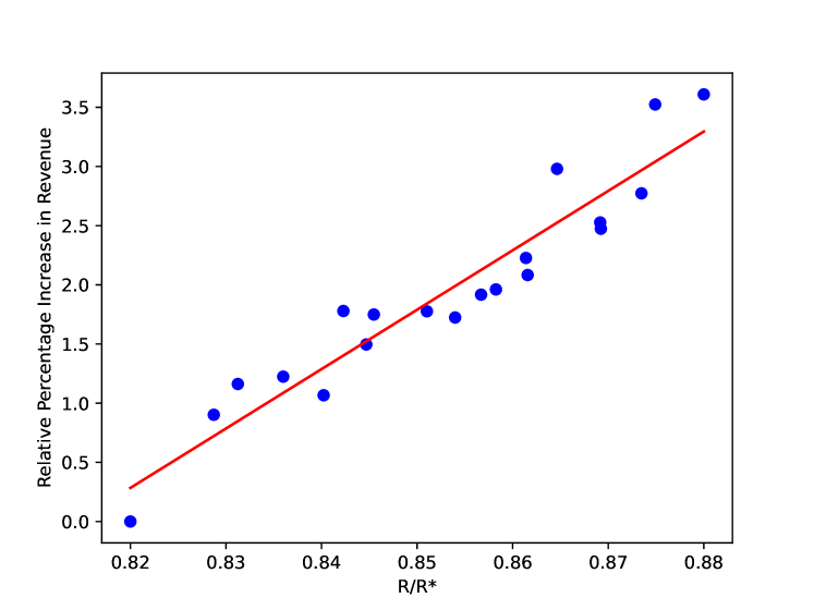
Figure 3. The relationship between $R/R^{*}$ and the relative increase in online revenue. The $R^{2}$ value is 0.902. The average deviation for the fitted data points is 0.243, and the maximum deviation is 0.483.

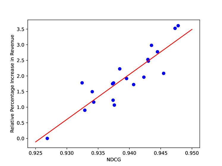
Figure 4. The relationship between $NDCG$ and the relative increase in online revenue. The $R^{2}$ value is 0.793. The average deviation for the fitted data points is 0.311, and the maximum deviation is 0.819.

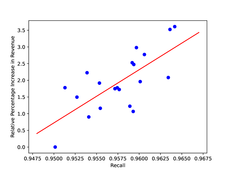
Figure 5. The relationship between $Recall$ and the relative increase in online revenue. The $R^{2}$ value is 0.509. The average deviation for the fitted data points is 0.534, and the maximum deviation is 1.139.

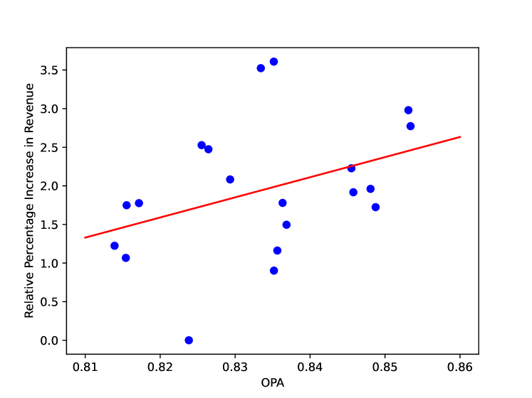
Figure 6. The relationship between $OPA$ and the relative increase in online revenue. The $R^{2}$ value is 0.140. The average deviation for the fitted data points is 0.634, and the maximum deviation is 1.690.

4.2. Scaling Laws of FLOPs and Offline Metric

In this section, we verify whether there is a scaling law for the model between computational effort and online revenue under the setting described in Section 3. Thanks to the strong linear correlation between $R/R^{*}$ and online revenue, we can transform the process of identifying the scaling law from online experiments to offline experiments. We trained 10 models with different MLP sizes offline, each for 10 days to ensure convergence. We then collected their converged $R/R^{*}$ metrics and calculated the FLOPs for each model to verify whether there is a scaling law for MLP models under our setting. We verify whether the collected data follows the Broken Neural Scaling Law (BNSL), which is a statistical law that has been widely validated by Caballero et al.((2023)) (Caballero et al., 2023) for many scaling behaviors of artificial neural networks in CV and NLP tasks. BNSL can be formulated as shown in Eq 6:

(6) $$\begin{split}R/R^{*}&=a+(b*FLOPs^{-c_{0}})\prod_{i=1}^{t}(1+(\frac{FLOPs}{d_{i}})^{1/f_{i}})^{(-c_{i}*f_{i})}\end{split}$$

where $a$,$b$,$c_{0}$,$c_{i}$,$f_{i}$ are parameters and $t$ is hyper-parameter of BNSL. $t$ characterizes the degrees of freedom of BNSL, and in practice, we typically take it as 6. The scaling factor is the FLOPs, and the dependent variable is our proposed offline metric $R/R^{*}$. We use basin-hopping (Wales and Doye, 1997) to fit the BNSL.

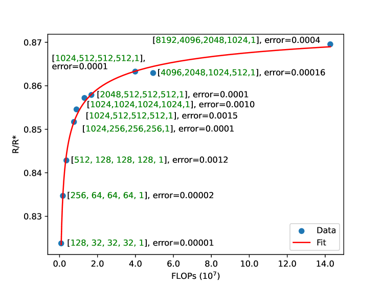
Figure 7. Scaling Performance regarding the FLOPs and $R/R^{*}$ of models. The size of the MLP network and the deviation between the fitted curve and the true values (referred to as the ”error”) are annotated in the figure. The $R^{2}$ value of the curve fitting is 0.996. Here [1024, 256, 256, 256, 1] indicates an MLP model with 5 layers, where the output sizes are 1024, 256, 256, 256, and 1, respectively. The total dimensions of input features for all models are 3328.

Figure 7 illustrates the curve obtained after fitting the BNSL, along with the original data points. The x-axis represents the scaling factor (FLOPs), and the y-axis represents the dependent variable ($R/R^{*}$). Each data point corresponds to an MLP model of a different size, with the number of layers and units per layer annotated in the figure. The $R^{2}$ value of the curve fitting is 0.996, indicating a strong correlation between the predicted values and the observed data points. Therefore, it provides strong evidence that there is indeed a Broken Neural Scaling Law for the MLP models under the typical scenario (referred to Section 3) of online advertisement retrieval. With this scaling law, we can predict or understand the scaling behavior of the MLP models.

It is important to note that the FLOPs in Figure 7 refer to the computational cost per user-ad pair (without customized optimization, e.g. the first-layer optimization), and the training data includes about 200 billion samples (namely user-ad pairs) and 20 billion impressions. We set the maximum FLOPs for the model to 143M FLOPs. The FLOPs range is not as wide as in NLP (Kaplan et al., 2020; Hoffmann et al., 2022). This is mainly because 143M FLOPs is about 20 times the FLOPs of our online base model, and a mature commercial system typically cannot easily allocate such a large amount of computing resources in the short term. Additionally, from the scaling laws validated in other scenarios, the marginal returns of increasing computational cost tend to decrease. Therefore, from the perspective of commercial applications of scaling law in advertising systems, which strongly focus on ROI, predicting model performance within the computational range of 0 to 143M FLOPs should be sufficient.

Thanks to the strong linear relationship between $R/R^{*}$ and online revenue, we can establish a prediction from FLOPs to online revenue. To further validate whether the accuracy of the FLOPs-to-revenue estimation meets the needs of model development and iteration, we deploy two models for 7 days, each with 10% of online traffic. The FLOPs for these models are 12.6M and 22.9M, respectively. Based on the scaling law, the estimated online revenue gains are 0.33% and 0.62%, while the actual online revenue increases are 0.38% and 0.69%, respectively. In our scenario, this accuracy is more than sufficient for guiding model development and iteration. Note that the MLP network size is [1024, 512, 512, 512, 1] for both models, while the dimensions of the input features are 5128 and 10128 (calculation details are shown in appendix B.1), respectively. This further indicates the generalization of the FLOPs-to-revenue estimation. We notice that the estimation errors of these two models are smaller than the average error of figure 3. This may be because the models in figure 3 were deployed for only one day, while these two models were deployed for 7 days, which means the observations of figure 3 would have higher variance.

4.3. Mapping Function from Model Settings to Computation Cost and FLOPs

Towards real-world applications, we need the scaling law of revenue and computation cost (namely machine cost), rather than the relationship of revenue and FLOPs. To this end, we should build a robust mapping function from FLOPs to computation cost without online deployment. Unfortunately, it’s intractable to give a certain formulation that maps the FLOPs to computation cost for general scenarios, since the actual computation cost is influenced by a multitude of factors including hardware specifications, software optimization, and so on. These factors can significantly vary across different environments, leading to highly non-linear and unpredictable relationships between FLOPs and actual costs.

To tackle this problem, we employ the parameters of model size to bridge the gap between FLOPs and computation cost. Determining the FLOPs of a model based on its size parameters is trivial. We use the tf.profiler API of TensorFlow to calculate the FLOPs for the forward pass of one user-ad pair. Thus, the main challenge lies in estimating the computation cost based on the model size parameters without online deployment. We propose two paradigms to identify the relationship between machine cost and model size parameters: 1) machine cost estimation based on software and hardware optimization experience, and 2) machine cost estimation based on offline simulation testing.

The first approach relies on professionals with deep expertise in optimizing software and hardware systems to minimize or avoid online deployment operations. They employ empirical methods to establish reliable correlations between model size and actual computation costs. For instance, Fang et al.((2024)) (Fang et al., 2024) estimated the machine cost for standard models like Transformers, trained using PyTorch on A100 GPUs, leveraging their expertise. However, in real-world advertising scenarios, customized training and serving frameworks (e.g., the first-layer optimization in section 3.4) and machine configurations introduce more complex nonlinearities between model size parameters and machine cost, increasing the complexity and difficulty of expertise-based cost estimation.

The second method is a more standardized, reproducible, and recommended approach for cost estimation. This method can be formalized as an algorithm, as shown in Algorithm 1. Thanks to the machine cost estimation tools (abbreviated as MCET) developed by our engineering team, which implement Algorithm 1, we can estimate the required machine numbers for tens of models without actually deploying or launching them. Using one machine with a single GPU, we can estimate the required number of machines for a single TensorFlow meta-file within half an hour. Combining this information with the unit price of the specified machine configuration, we can accurately calculate the expected machine cost. It is important to note that for training and serving cost estimation, the algorithm should be executed using the meta files specific to the training and serving process, respectively. For training cost estimation, labels are randomly constructed. This approach not only saves time but also provides a reliable and efficient way to estimate computation costs for model deployment and iteration.

Algorithm 1 Cost Estimation by Offline Simulation Testing

0:  The number $n$ of models (denoted as $n$), and meta files of the models (denoted as $\{meta_{i}|0\leq i<n\}$). One specified machine $\mathcal{MH}$ for online serving. The machine number $req_{0}$ of the online base model $M_{0}$. The desired response time limit $T_{\text{limit}}$.

0:  The estimated machine number of each model for online serving, denoted as $\{req_{i}|1\leq i<n\}$.

1:  Initialize an empty list $results$ to store the results.

2:  Simulate the execution of the base model $M_{0}$ using the specified hardware configuration $\mathcal{MH}$.

3:  Measure the QPS ($QPS_{0}$) of the base model $M_{0}$ under the given response time limit $T_{\text{limit}}$, with the input being randomly initialized, fixed-length tensors.

4:  Calculate the total QPS capacity of the base model setup: $QPS_{\text{total}}=req_{0}\times QPS_{0}$.

5:  for $i=1$ to $n-1$ do

6:     Load the meta file $meta_{i}$ of the $i$-th model.

7:     Simulate the model’s execution using the specified hardware configuration $\mathcal{MH}$.

8:     Measure the QPS ($QPS_{i}$) of the $i$-th model under the given response time limit $T_{\text{limit}}$, with the input being randomly initialized, fixed-length tensors.

9:     Calculate the required number of machines for the $i$-th model: $req_{i}=\frac{QPS_{\text{total}}}{QPS_{i}}$.

10:     Append the result $req_{i}$ to the $results$ list.

11:  end for

12:  return  $results$

5. Applications in Model Designing and Resource Allocation

In this section, we show two real-world applications of the scaling laws identified by the paradigm in section 4 in the advertising system of Kuaishou Technology. To facilitate the description, we first define the following notations:

• $\mathcal{SP}=[a_{0},a_{1},\ldots,a_{n}]$: A list representing the size parameters of an MLP, where $a_{0}$ denotes the dimension of the MLP input, and $a_{1}$ to $a_{n}$ denote the output dimensions of each layer. Let us denote the TensorFlow meta file generated from the MLP model configured with $\mathcal{SP}$ as $meta_{\mathcal{SP}}$.

• $F(\mathcal{SP})$: The FLOPs of the network with size parameters $\mathcal{SP}$.

• $G$: The mapping function from $R/R^{*}$ to the expected online revenue, which is a linear function.

• $BNSL$: The mapping function from FLOPs to $R/R^{*}$, which follows the form given in Equation 6.

• $MCET$: The tool (function) used to estimate machine costs, where $MCET(meta_{\mathcal{SP}})$ represents the estimated machine cost for deploying an MLP with size parameters $\mathcal{SP}$.

where $G$, $BNSL$, $F$ and $MCET$ are obtained by referring to section 4.1, section 4.2, and section 4.3, respectively.

5.1. ROI-Constrained Model Designing

For a commercial company, there is usually a standard regarding ROI. Specifically, for an advertising system, we aim for the return on investment (ROI) from the machine to be no less than $\lambda$, where $\lambda$ is typically determined by management based on the company’s operating conditions.

Given a specific MLP model with size parameters $\mathcal{SP}$, the ROI of the model can be estimate by Eq 7:

(7) $$\begin{split}ROI&=\frac{G(BNSL(F(\mathcal{SP})))}{MCET(meta_{\mathcal{SP}})}\end{split}$$

Thus, given the ROI constraint, we can find the approximate optimal model size by solving the following optimization problem:

(8) $$\begin{split}\max_{\mathcal{SP}}&\quad G(BNSL((F(\mathcal{SP}))))\\ \text{s.t. }&\quad\frac{G(BNSL(F(\mathcal{SP})))}{MCET(meta_{\mathcal{SP}})}\geq\lambda\\ \end{split}$$

Notice that $\mathcal{SP}$ is a vector where each element represents the number of units in each layer of the MLP. As each element in $\mathcal{SP}$ increases, $F(\mathcal{SP})$, $BNSL(\mathcal{SP})$, and $G(BNSL(\mathcal{SP}))$ also increase, indicating that $F$, $BNSL$, and $G$ are monotonically increasing functions. However, $MCET$ is not a monotonic function and is typically a complex mapping, making the problem non-convex and unsolvable analytically or through binary search.

For the functions in Eq 8, the most time-consuming part is the computation of $MCET(\mathcal{SP})$, which relies on a simulation testing tool. Fortunately, even the computation of $MCET$ does not have a high time and resource cost, allowing us to perform a grid search on this problem. We use 10 T4-GPU machines to run the grid search of about 1000 configurations and find an approximate optimal solution in about two days. Due to space limitations, details of the grid search settings are introduced in appendix B.1.

With the specific ROI constraint of Kuaishou Technology, we solve the approximate optimal size of our foundation MLP model, the $\mathcal{SP}$ of the online base model and the solved model are [3328, 1024, 256, 256, 256, 1] and [16128, 1024, 512, 512, 512, 1], the new model has brought about a 0.85% increase in revenue. Such an improvement is considered significant in our advertising scenario. Without the scaling law, it would be nearly impossible to test the ROI of hundreds of model configurations through online deployment. The time and resource costs of deploying so many models would far outweigh the incremental revenue from the optimized model derived using the scaling law.

5.2. Multi-scenario Resource Allocation

There are often different scenarios that use different models in online advertising systems, such as using different models for different stages and ad placements. Taking different stages as an example, we show the practice of the optimization in multi-scenario resource allocation via scaling law.

Let us assume there are $t$ scenarios, with a total machine cost of $B$. We want to maximize the total revenue through resource allocation across multiple scenarios without increasing the total machine cost, while ensuring that each scenario’s ROI is greater than 1. We can formulate the optimization problem as Eq 9:

(9) $$\begin{split}\max_{\{\mathcal{SP}_{i}\mid 0\leq i<t\}}&\sum_{i=0}^{t-1}G(BNSL(F(\mathcal{SP}_{i})))\\ \text{s.t. }&\sum_{i=0}^{t-1}MCET(meta_{\mathcal{SP}_{i}})\leq B\\ \text{s.t. }&\forall i\in\{0,\ldots,t-1\},\frac{G(BNSL(F(\mathcal{SP}_{i})))}{MCET(meta_{\mathcal{SP}_{i}})}\geq 1\\ \end{split}$$

This problem can be solved using the same approach as described in sub-section 5.1. The computational complexity of the grid search would be about $t$ times the complexity mentioned in Eq. 8, with the majority of the computation concentrated in the calculation of MCET. In our case, we consider the Matching and Pre-ranking stages as separate scenarios, so $t=2$. Even with $t=2$, we can still use a grid search to solve the problem exhaustively. Due to the initially suboptimal resource allocation, this optimization resulted in a significant 2.8% increase in online revenue. If $t$ is large in practice, making the grid search computationally infeasible, we can employ heuristic information to prune the search space or consider only proportional scaling of the base model. Due to space limitations, more details of multi-scenario resource allocation are shown in appendix B.2.

6. Conclusion

We have systematically studied the scaling laws for online advertisement retrieval and validated the existence of scaling laws in a typical learning-to-rank task with MLP models. To address the challenge of the high cost in time and resources of obtaining scenario-specific scaling law parameters in industrial applications, we propose a lightweight paradigm that transforms most online experiments into low-cost offline experiments through the offline metric R/R* and the machine cost estimation tool. Our work showcases the practical application of the scaling law in optimizing model design under ROI constraints and efficient resource allocation across multiple scenarios in the Kuaishou advertising system, thereby bringing significant commercial value. We also discuss the limitations of our study and outline potential areas for future research in appendix C in the context of scaling laws in online advertisement retrieval.

Appendix A More Details about Online Training and Serving

Figure 8 illustrates the pipeline of online training and online serving in the Kuaishou advertising system and the details of ”first-layer optimization” mentioned in section 3.4. The advertising system records logs in real-time for each ad exposure, including the features and labels of the training samples. The downstream training engine reads training data from Kafka storage in real-time and performs online training to optimize the model. Every 20 minutes, the training engine exports the latest model parameters to HDFS for secure storage. Meanwhile, the prediction server periodically polls HDFS to check for new model parameters and updates the local model parameters when a new version is available.

First-layer optimization is an optimization technique designed for MLP models. This technique transforms the computation of the first layer from $FFN(\text{concat}(emb_{user},emb_{ad}))$ (referred to as $FL_{\text{naive}}$) to $FFN(emb_{user})+FFN(emb_{ad})$ (referred to as $FL_{\text{opt}}$). The transformation yields equivalent results but significantly reduces computational overhead. This optimization is applied to the pre-ranking models of the Kuaishou advertising system, where each impression involves evaluating 1500 candidate ads. In this context, for each impression, there is one user embedding ($emb_{user}$) and 1500 ad embeddings ($emb_{ad}$). The operations concat and $+$ are broadcast operations, meaning they can be applied element-wise across arrays of different shapes. Here, the term ”concat” refers to a logical operation with broadcasting properties, which in practice can be implemented using a combination of tf.tile and tf.concat in TensorFlow. By adopting the optimized form $FL_{\text{opt}}$, we can save a substantial amount of computation. To further enhance efficiency, we have developed a scheduled precomputation service called the “Embedding Producer.” This service caches the $FFN(emb_{ad})$ values for all valid ads. It is a CPU-based service that is triggered by model update events and the insertion of new ads. This caching mechanism ensures that the precomputed values are readily available, reducing the computational overhead of the pre-ranking models.

For the training procedure of Pre-ranking models, we have also implemented the first-layer optimization. However, during training, each impression typically involves only about 10 ads, which results in far fewer computational savings compared to the pre-ranking service. For both training and serving, we use T4 GPUs, with each T4 GPU machine equipped with 128 CPU cores. During training, we utilize an asynchronous distributed training framework to improve efficiency and scalability. Both the training and serving frameworks are developed based on TensorFlow. Matching models in our system use the twin-tower structure, inheriting all settings except the first-layer optimization. The inner product of the user and ad tower is directly calculated by brute force for online serving, and no approximate search algorithm such as FAISS is employed.

Figure 8. The pipeline of online training and serving, and details of the first layer optimization for Pre-ranking models.

Appendix B More Details about the Applications of Scaling Law

B.1. ROI-Constrained Model Designing

We set an upper limit on the model FLOPs to 143M and set the step size of the grid search as 16 and 128 for the feature embedding dimensions and the unit number of MLP layers, respectively. This larger step size is chosen because smaller increments have minimal impact on the total FLOPs and result in negligible increases in expected revenue according to the scaling law. The feature embedding dimension ($emb\_dim$) in the grid search starts at 16. The input size of MLP models is determined by multiplying the $emb\_dim$ by the number of sparse features, which is 200 in our experiments, plus an additional 128-dimensional dense feature. For the MLP layers (excluding the output layer, which is fixed at 1), the number of units starts at 128, with the constraint that the number of units in any layer does not exceed the number of units in the previous layer. The size of the first layer outputs does not exceed 1024, because this is the storage limit of the embedding producer. Additionally, we enforce that the number of units in any layer (except the output layer) is at least 1/20 of the number of units in the previous layer as the reason discussed in appendix C.1. We used 10 T4-GPU machines to perform a grid search over approximately 1000 configurations and found an approximate optimal solution in about two days.

B.2. Multi-scenario Resource Allocation

We adopted an MLP model for the Pre-ranking stage and a twin-tower model for the Matching stage. Through offline experiments, we obtained the key functions (including $G$, $BNSL$, etc.) in the scaling laws for both the Matching and Pre-ranking stages using our proposed paradigm. Due to the different model architectures, their machine costs vary in the same size. We used the machine cost estimation tool to additionally measure the machine costs of the twin-tower model at different sizes. Similarly to the estimation of the MLP model, we solved the estimated machine costs of approximately 1000 different sizes of twin-tower models based on the algorithm 1 using 10 T4-GPU machines for about 2 days.

Appendix C Limitations and Future Work

C.1. Optimal Model Designing with Given FLOPs

One remaining question is how to give optimal unit distributions of layers under a given FLOPs. Typically, in advertising models, the size of the bottom layer is the largest, gradually decreasing in the upper layers. We believe that as long as the difference in the number of units between adjacent layers is within a reasonable range, the performance impact should be negligible. To explore this, we conducted preliminary experiments, such as testing a model with the size [3328, 1024, 32, 32, 32, 1]. We found that when the unit allocation is unreasonable, the model performance significantly degrades compared to a reasonable one. Our empirical experience suggests that, except for the output layer, the difference in the number of units between adjacent layers should not exceed 20. Models designed following this principle generally conform to the BNSL. More in-depth conclusions are left for future work and are beyond the scope of this paper.

C.2. New Foundation Models and Joint Laws

While the transformer has become a foundational model in the NLP domain, capable of being applied to almost all tasks and scenarios, the recommendation and advertising fields lack such a foundation model. This absence means that the scaling law parameters obtained in one scenario cannot be readily reused in another. In addition, our scaling laws show that the benefits of increasing FLOPs converge to zero much more rapidly. It’s different from the conclusion in NLP area, where increasing the FLOPs by an order of magnitude typically results in consistent performance improvements. An important reason might be that MLP models in online advertisement retrieval are not as effective foundation models as transformers in NLP. However, it is worth noting that transformers do not universally outperform MLPs in all advertising scenarios, especially when considering the ROI of the machine. Given these challenges, developing more advanced and universal foundation models with better scaling performance (e.g., recent works (Zhai et al., 2024; Zhang et al., 2024b; Guo et al., 2024)) is a crucial direction for future research in online advertisement.

Additionally, obtaining joint laws considering multiple factors such as data, model size, and computational resources is significantly more costly in industrial advertising settings than obtaining single-variable scaling laws. Developing a cost-effective method for deriving joint laws is therefore an important area for future investigation. The high cost of obtaining joint laws is also one of the motivations behind our exploration of unified foundation models.

References

- (1)
- Achiam et al. (2023) Josh Achiam, Steven Adler, Sandhini Agarwal, Lama Ahmad, Ilge Akkaya, Florencia Leoni Aleman, Diogo Almeida, Janko Altenschmidt, Sam Altman, Shyamal Anadkat, et al. 2023. Gpt-4 technical report. arXiv preprint arXiv:2303.08774 (2023).
- Bauer et al. (2024) Christine Bauer, Eva Zangerle, and Alan Said. 2024. Exploring the landscape of recommender systems evaluation: Practices and perspectives. ACM Transactions on Recommender Systems 2, 1 (2024), 1–31.
- Brown (2020) Tom B Brown. 2020. Language models are few-shot learners. arXiv preprint ArXiv:2005.14165 (2020).
- Caballero et al. (2023) Ethan Caballero, Kshitij Gupta, Irina Rish, and David Krueger. 2023. Broken Neural Scaling Laws. In ICLR.
- Chen et al. (2017) Ruey-Cheng Chen, Luke Gallagher, Roi Blanco, and J. Shane Culpepper. 2017. Efficient Cost-Aware Cascade Ranking in Multi-Stage Retrieval. In SIGIR. 445–454.
- Covington et al. (2016) Paul Covington, Jay Adams, and Emre Sargin. 2016. Deep neural networks for youtube recommendations. In RecSys. 191–198.
- Duchi et al. (2011) John Duchi, Elad Hazan, and Yoram Singer. 2011. Adaptive subgradient methods for online learning and stochastic optimization. JMLR 12, 7 (2011).
- Fang et al. (2024) Yan Fang, Jingtao Zhan, Qingyao Ai, Jiaxin Mao, Weihang Su, Jia Chen, and Yiqun Liu. 2024. Scaling laws for dense retrieval. In SIGIR. 1339–1349.
- Gallagher et al. (2019) Luke Gallagher, Ruey-Cheng Chen, Roi Blanco, and J. Shane Culpepper. 2019. Joint Optimization of Cascade Ranking Models. In WSDM. 15–23.
- Grover et al. (2019) Aditya Grover, Eric Wang, Aaron Zweig, and Stefano Ermon. 2019. Stochastic Optimization of Sorting Networks via Continuous Relaxations. In ICLR.
- Guo et al. (2024) Xingzhuo Guo, Junwei Pan, Ximei Wang, Baixu Chen, Jie Jiang, and Mingsheng Long. 2024. On the Embedding Collapse when Scaling up Recommendation Models. In ICML.
- He et al. (2015) Kaiming He, Xiangyu Zhang, Shaoqing Ren, and Jian Sun. 2015. Delving deep into rectifiers: Surpassing human-level performance on imagenet classification. In ICCV. 1026–1034.
- He et al. (2014) Xinran He, Junfeng Pan, Ou Jin, Tianbing Xu, Bo Liu, Tao Xu, Yanxin Shi, Antoine Atallah, Ralf Herbrich, Stuart Bowers, et al. 2014. Practical lessons from predicting clicks on ads at facebook. In Proceedings of the eighth international workshop on data mining for online advertising. 1–9.
- Hestness et al. (2017) Joel Hestness, Sharan Narang, Newsha Ardalani, Gregory Diamos, Heewoo Jun, Hassan Kianinejad, Md Mostofa Ali Patwary, Yang Yang, and Yanqi Zhou. 2017. Deep learning scaling is predictable, empirically. arXiv preprint arXiv:1712.00409 (2017).
- Hoffmann et al. (2022) Jordan Hoffmann, Sebastian Borgeaud, Arthur Mensch, Elena Buchatskaya, Trevor Cai, Eliza Rutherford, Diego de Las Casas, Lisa Anne Hendricks, Johannes Welbl, Aidan Clark, et al. 2022. Training compute-optimal large language models. arXiv preprint arXiv:2203.15556 (2022).
- Hornik et al. (1989) Kurt Hornik, Maxwell Stinchcombe, and Halbert White. 1989. Multilayer feedforward networks are universal approximators. Neural networks 2, 5 (1989), 359–366.
- Huang et al. (2022) Siguang Huang, Yunli Wang, Lili Mou, Huayue Zhang, Han Zhu, Chuan Yu, and Bo Zheng. 2022. MBCT: Tree-Based Feature-Aware Binning for Individual Uncertainty Calibration. In WWW. 2236–2246.
- Isik et al. (2024) Berivan Isik, Natalia Ponomareva, Hussein Hazimeh, Dimitris Paparas, Sergei Vassilvitskii, and Sanmi Koyejo. 2024. Scaling laws for downstream task performance of large language models. arXiv preprint arXiv:2402.04177 (2024).
- Kaplan et al. (2020) Jared Kaplan, Sam McCandlish, Tom Henighan, Tom B Brown, Benjamin Chess, Rewon Child, Scott Gray, Alec Radford, Jeffrey Wu, and Dario Amodei. 2020. Scaling laws for neural language models. arXiv preprint arXiv:2001.08361 (2020).
- Qin et al. (2022) Jiarui Qin, Jiachen Zhu, Bo Chen, Zhirong Liu, Weiwen Liu, Ruiming Tang, Rui Zhang, Yong Yu, and Weinan Zhang. 2022. RankFlow: Joint Optimization of Multi-Stage Cascade Ranking Systems as Flows. In SIGIR. 814–824.
- Qin et al. (2021) Zhen Qin, Le Yan, Honglei Zhuang, Yi Tay, Rama Kumar Pasumarthi, Xuanhui Wang, Michael Bendersky, and Marc Najork. 2021. Are Neural Rankers still Outperformed by Gradient Boosted Decision Trees?. In ICLR.
- Sheng et al. (2023) Xiang-Rong Sheng, Jingyue Gao, Yueyao Cheng, Siran Yang, Shuguang Han, Hongbo Deng, Yuning Jiang, Jian Xu, and Bo Zheng. 2023. Joint optimization of ranking and calibration with contextualized hybrid model. In KDD. 4813–4822.
- Shin et al. (2023) Kyuyong Shin, Hanock Kwak, Su Young Kim, Max Nihlén Ramström, Jisu Jeong, Jung-Woo Ha, and Kyung-Min Kim. 2023. Scaling law for recommendation models: Towards general-purpose user representations. In AAAI. 4596–4604.
- Vaswani et al. (2017) Ashish Vaswani, Noam Shazeer, Niki Parmar, Jakob Uszkoreit, Llion Jones, Aidan N. Gomez, Lukasz Kaiser, and Illia Polosukhin. 2017. Attention is All you Need. In NeurIPS. 5998–6008.
- Wales and Doye (1997) David J Wales and Jonathan PK Doye. 1997. Global optimization by basin-hopping and the lowest energy structures of Lennard-Jones clusters containing up to 110 atoms. The Journal of Physical Chemistry A 101, 28 (1997), 5111–5116.
- Wang et al. (2011) Lidan Wang, Jimmy Lin, and Donald Metzler. 2011. A cascade ranking model for efficient ranked retrieval. In SIGIR. 105–114.
- Wang et al. (2018) Xuanhui Wang, Cheng Li, Nadav Golbandi, Michael Bendersky, and Marc Najork. 2018. The lambdaloss framework for ranking metric optimization. In CIKM. 1313–1322.
- Wang et al. (2024) Yunli Wang, Zhiqiang Wang, Jian Yang, Shiyang Wen, Dongying Kong, Han Li, and Kun Gai. 2024. Adaptive Neural Ranking Framework: Toward Maximized Business Goal for Cascade Ranking Systems. In WWW. 3798–3809.
- Zangerle and Bauer (2022) Eva Zangerle and Christine Bauer. 2022. Evaluating recommender systems: survey and framework. Comput. Surveys 55, 8 (2022), 1–38.
- Zhai et al. (2024) Jiaqi Zhai, Lucy Liao, Xing Liu, Yueming Wang, Rui Li, Xuan Cao, Leon Gao, Zhaojie Gong, Fangda Gu, Michael He, et al. 2024. Actions speak louder than words: Trillion-parameter sequential transducers for generative recommendations. In ICML.
- Zhang et al. (2024b) Buyun Zhang, Liang Luo, Yuxin Chen, Jade Nie, Xi Liu, Daifeng Guo, Yanli Zhao, Shen Li, Yuchen Hao, Yantao Yao, et al. 2024b. Wukong: Towards a Scaling Law for Large-Scale Recommendation. In ICML.
- Zhang et al. (2024a) Gaowei Zhang, Yupeng Hou, Hongyu Lu, Yu Chen, Wayne Xin Zhao, and Ji-Rong Wen. 2024a. Scaling Law of Large Sequential Recommendation Models. In RecSys. 444–453.