Spinning Particle Dynamics and ISCO in Covariant Loop Quantum Gravity
Abstract
In this paper, we investigate the motion of spinning particles in the background of covariant loop quantum gravity black holes, focusing on two distinct effective metric solutions. Both metrics incorporate a quantum parameter , which quantifies the corrections from loop quantum gravity. When approaches zero, the spacetime reduces to the classical Schwarzschild solution. Using the pole-dipole approximation, we derive the equations of motion for spinning particles, accounting for the spin-curvature coupling. Our analysis reveals significant deviations in the behavior of the Innermost Stable Circular Orbit (ISCO) due to quantum effects. In the first effective metric, as increases, the ISCO’s radial position shifts, and for sufficiently large values of (greater than 4.55), the ISCO disappears, allowing particles to hover above the black hole. In contrast, in the second metric, ISCOs persist even for large values of , albeit with a more restrictive spin range. These findings highlight the impact of loop quantum gravity corrections on the dynamics of spinning particles and provide insights into potential observational consequences for gravitational wave detections.
I introduction
General relativity, as extensively discussed in both popular science literature and specialized textbooks, has profoundly transformed our understanding of the nature of spacetime. Yet, from a practical standpoint, it is equally significant for offering a method of studying celestial orbits that stands in stark contrast to Newtonian mechanics. This distinction is especially prominent in regions of intense gravitational fields, such as near black holes, where orbiting bodies with intrinsic spin follow trajectories markedly different from Newtonian predictions [1]. Furthermore, the entire motion is often accompanied by the radiation of gravitational waves [2, 3, 4, 5, 6]—a phenomenon completely absent in Newtonian gravity. The detection of gravitational waves by the LIGO and Virgo collaborations in 2016 marked a revolutionary advancement in astrophysics, providing direct evidence of binary black hole mergers [7, 8]. As two black holes inspiral towards each other, driven by the emission of gravitational radiation, they gradually lose orbital energy, moving closer until they reach the innermost stable circular orbit (ISCO) of the system. At this critical radius, the orbit transitions from stable to unstable, leading to a rapid plunge and ultimately, the merger of the black holes. This final stage is characterized by a burst of gravitational waves, which LIGO detected with remarkable precision.
Understanding the ISCO is therefore essential for interpreting the late inspiral phase of binary black hole mergers, as it dictates the point at which stable circular motion ceases, and the plunge phase begins. Since this concept entered the academic spotlight, many works have analyzed the ISCO in various spacetime configurations [9]-[26]. These models, in turn, allow for the extraction of physical parameters, such as mass and spin, from gravitational wave data, thus linking theoretical predictions to observable quantities. Building upon these works, Refs. [27]-[45] considered a more realistic scenario: celestial bodies orbiting black holes possess intrinsic spin. The effects of spin on the trajectory and the radius of the ISCO are taken into account, which is one of the central concerns of this study. The most fundamental change brought about by spin is the deformation of the equation of motion. Specifically, the particle no longer travels along the geodesic of spacetime but instead deviates due to the coupling effect between the spacetime curvature and its spin. Typically, the equation is considered under the pole-dipole approximation, where the particle’s 4-momentum and 4-velocity are no longer parallel. Consequently, for a timelike 4-momentum, the particle’s 4-velocity may become spacelike. Therefore, when considering the equation of motion, we must also incorporate the timelike constraint. In [36], the radius of ISCO for spinning particles in KN black hole has been studied, and it has been found to be smaller than that of non-spinning particles in the same spacetime [27].
However, despite General Relativity’s undefeated record in facing rigorous experimental tests, there remains an underlying skepticism that it fully captures the essence of gravity. This doubt stems from its logical discord with the worldview of quantum theory. On a superficial level, the concept of a test particle’s trajectory conflicts with the Heisenberg uncertainty principle. On a deeper level, the existence of an irrevocable one-way boundary—the event horizon of a black hole—challenges the unitarity of quantum theory in such backgrounds, destabilizing the very foundation of predictability in physics. This dilemma is epitomized by the black hole information paradox [46]-[50]. Only a self-consistent and complete theory of quantum gravity could fundamentally reconcile these two experimentally robust yet seemingly incompatible theories.
Loop quantum gravity (LQG) is one such attempt to achieve this reconciliation [51]-[58]. The core idea of this theory is to quantize the very geometry of spacetime, representing the gravitational field through discrete “loops” or “rings.” Spacetime is conceptualized as having a discrete, network-like structure, implying that at extremely small scales (the Planck scale), it is not continuous but composed of fundamental units. From a semiclassical perspective, loop quantum gravity offers quantum corrections to some well-known black hole solutions in general relativity [62, 63, 64, 65, 66]. However, most of these solutions encounter the so-called ”covariance” issue which is crucial for studying geodesics and perturbations [67]. Since the solution even with small perturbations are usually no longer the solution of the same quantum corrected Hamiltonian constraint. To overcame this issue, recently, black hole solutions compatible with quantum theory, retaining the diffeomorphism invariance while employing the Hamiltonian formalism are constructed for a vacuum, spherically symmetric system [68, 69]. And hence addressing the covariance problem under this setup. This paper focuses on a semiclassical loop quantum gravity metric explored in [68, 69]. Based on this foundation, we will investigate the quantum gravitational effects on the orbital corrections of test particles orbiting black holes.
The structure of this paper is as follows: In Section 2, we briefly introduce two effective metrics derived from covariant loop quantum gravity, and provide the equations of motion for spinning particles under the pole-dipole approximation in these backgrounds, along with the corresponding timelike constraint. In Section 3, we focus on the first metric, analyze the effective potential for the motion of spinning particles in this spacetime, identify the ISCO, and discuss the characteristics of the ISCO parameters, comparing them with those in purely classical spacetime. In Section 4, we apply the same approach to analyze the ISCO in the background of the second metric. Finally, in Section 5, we summarize the results of this paper and offer a range of prospects for future work.
II The Equation of Motion of Spinning Particles
II.1 Black hole solution of covariant 4-Spacetime Theories
In this subsection, we will provide a brief review of the black hole solutions in [68]. To maintain diffeomorphism invariance, two different forms of the effective Hamiltonian that satisfy this condition lead to two corresponding metric solutions via the standard procedure [70]. The resulting 4-dimensional line element of a black hole in Boyer-Lindquist coordinates reads as
| (1) |
with solution 1:
| (2) | |||||
| (3) |
and solution 2:
| (4) | |||||
| (5) |
where is the mass of the covariant black hole. The quantum parameter , with being the Barbero-Immirzi parameter and the Planck length. Here, we use the normalized quantum parameter after loop quantization.
Solution 1 is similar in form to a Reissner-Nordström (RN) black hole with a small charge. The equation has two positive roots, given by and , where . Similar to the characteristics of an RN black hole, these two roots correspond to the outer horizon and inner horizon. The solution 2 features a transition surface [68, 69], which is a spacelike surface marking the boundary between the black hole and white hole regions. This is a common phenomenon in loop quantum gravity (LQG) black hole solutions, replacing the perplexing black hole singularity with a continuous and smooth spacetime transition region. Another intriguing aspect of this transition surface lies in its potential to address the black hole information paradox. Simply put, the information of matter falling into the black hole is not lost; instead, it traverses the transition surface and is eventually released in another spacetime region. Both solutions represent modifications of the Schwarzschild metric, and as approaches zero, indicating minimal quantum gravitational effects, both solutions reduce to the classical vacuum spherically symmetric solution.
II.2 Equation of motion of spinning particles
To obtain a more convenient framework for studying the trajectory of particles in black hole spacetimes, we assume here that the particles in focus have masses much smaller than that of the black hole. Thus, they may be treated as test particles, devoid of any backreaction on the background spacetime. In principle, any test particle in spacetime should follow a geodesic path. However, if the particle possesses spin, its trajectory deviates, governed instead by the Mathisson-Papapetrou-Dixon (MPD) equations, which is derived under the pole-dipole approximation [1, 43],
| (6) | |||||
| (7) |
where is the spin tensor that is antisymmetric, is the Riemann tensor, is the 4-momentum, and is the tangent 4-vector along the trajectory. serve as the affine parameter of the curve. A set of supplementary condition are also needed [71]
| (8) |
to eliminate the remaining undetermined degrees of freedom, which are related to the center of mass of a spinning particle and are observer-dependent. Thus the condition is not unique [71] and may yield different ISCO radius results [29]. Using the spin tensor and 4-momentum, we can define the mass and spin of the particle as follows:
| (9) | |||||
| (10) |
(9) means that is always timelike along the trajectory. The affine parameter can be normalized as
| (11) |
Hence, we could get the difference between 4-momentum and 4-velocity as follows [30]:
| (12) |
We observe that the 4-velocity and 4-momentum of the test particle are not parallel, which is an another effects of spin.
For the sake of simplicity, we prioritize the motion in the equatorial plane where and are vanishing. We introduce a spin vector to express the component of
| (13) |
where is the antisymmetric tensor with . One find all the components of the spin vector are trivial except
| (14) |
Hence, the expression of the antisymmetric spin tensor can be re-described as
| (15) | |||||
| (16) | |||||
| (17) |
Now we get the difference between the 4-momentum and 4-velocity as
| (18) | |||||
| (19) | |||||
| (20) |
where
| (21) |
| (22) | |||||
| (23) | |||||
| (24) |
For the spinning particles, the conserved quantities in this spacetime can be given as
| (25) |
where is the Killing vector. Note that the Killing vectors are and . From it, we acquire the energy and the angular momentum in the equatorial plane
| (26) | |||||
| (27) |
We also define orbital angular momentum as which will be useful in the following section. By inverting the above relations and combining with (15)-(17), we obtain
| (28) | |||||
| (29) |
It is worth noting that the missing term can be obtained by the normalization condition of the 4-momentum in (9):
| (30) |
Without loss of generality, we use dimensionless parameters instead of the original parameters, as follows:
| (31) |
For simplicity of expression, we omit the tilde on dimensionless parameters; for example, will represent in the following parts of the paper.
II.3 Timelike condition of the orbits
It can be seen in (9) that the momentum naturally follows the trajectory in a timelike manner. However,(12) reveals that the velocity does not always align with the momentum, and under the pole-dipole approximation [43] it may lead to some highly unphysical conclusions, for example, the particle’s velocity exceeding the speed of light. To make sure the orbits exist physically, a superluminal constraint must be imposed on the velocity [31], given by
| (32) |
The emergence of this superluminal issue arises due to the polar-dipole approximation in the construction of the MPD equations. If non-minimal spin-gravitational interactions are taken into account, as suggested by [32, 33, 34, 35], the superluminal problem can be circumvented.
III The Motion of Spinning Particles in the solution 1 Spacetime
III.1 Effective potential
The spherical symmetry of the spacetime background allows the orbital motion in the equatorial plane to be treated as a central force problem. As in Newtonian dynamics, where an effective potential is commonly used to study particle motion, an effective potential can similarly be introduced in general relativity to analyze the behavior of test particles in a fixed spacetime background. By writing the momentum (30) in the following way as
| (33) |
where
| (34) | |||||
| (35) | |||||
| (36) | |||||
| (37) |
the effective potential of the background field for the particle can be defined as
| (38) | |||||
| (39) |
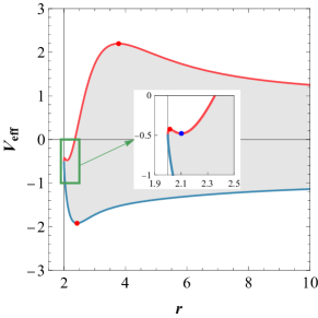
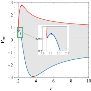
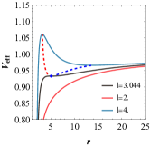
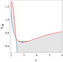
It has two branches. The negative branch is often neglected in typical ISCO effective potential studies due to its tendency to fall below zero [36, 37]. However, as shown in Fig. 1, with appropriate parameter values(for example , and in the right plot), can also attain positive values for some small radius region. Thus we consider the negative branch when analyse the circular orbits. Since is always greater than zero, the effective potential must satisfy or at any radial position . It means that in the radial range where the particle actually moves, such as within to , the total energy of the particle cannot lie within the shaded region bounded by the and curves in Fig 1.
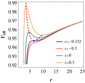
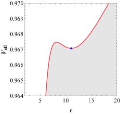
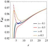
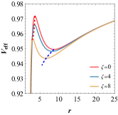
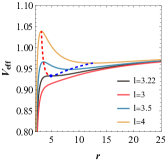
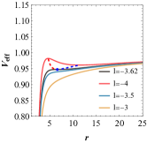
Now we focus on the variation of with respect to the radial coordinate , as illustrated in Fig. 2. Subplot (a) shows the effect of spin on , with fixed values and . As varies from to , the peak and shape of undergo noticeable changes, demonstrating how spin can alter stability in the particle’s orbit. The smaller the spin, the lower the position of the corresponding curve. For the same curve, as the distance from the central force field increases, the effective potential first rises to a peak, then decreases, and finally turns upward again. The overall trend of the curve in Subplot (b) is similar to that in (a), but it highlights the role of in , where and are kept constant. The values of range from to , showing that the effect of LQG have on the effective potential profile. As increases, the overall position of the curve shifts upward, and the peak becomes sharper. Subplot (c) and (d) examines how changes in angular momentum parameter , when taking positive and negative value, affect , holding and fixed. It could be seen that as the absolute value of increases, the effective potential rises. When the absolute value of is relatively small, such as , the entire curve no longer exhibits roller-coaster-like fluctuations but instead rises smoothly.
III.2 ISCO
In this subsection we turn our attention to the Innermost Stable Circular Orbit. As the term “circular” implies, the trajectory of a particle in the ISCO is perfectly round, which necessitates that the radial velocity vanishes: . This criterion places a fundamental constraint on the effective potential, demanding that it satisfy
| (40) |
This condition also implies . Thus, the effective potential must also fulfill the following requirements:
| (41) |
Beyond the requirements for zero radial velocity and acceleration, “innermost” implies a boundary in stability: no further stable circular orbit exists closer to the central mass [38]. Thus, the ISCO represents the critical point at which the effective potential reaches a delicate balance between a local maximum and minimum, intersecting precisely at this juncture. This condition can be expressed as:
| (42) |
Therefore, for a given expression, the orbital position of the ISCO can be uniquely determined using the three conditions mentioned above.
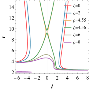
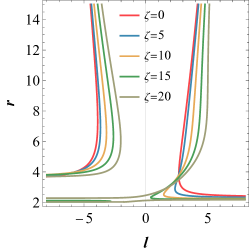
As seen in Fig. 2, typically has two extremal points: one near the black hole, which is an unstable point, and another at a larger radius, which is stable. They both represent circular orbits, satisfying (40). In Fig. 3, we plot the variation of these two extremal points in the plane for different or . As shown in the left panel, when is set to and is small, the curve resembles the results in [36], where the upper part of each turning point of the curve represents the stable extremal point’s in Fig. 2, while the lower part represents the unstable point. The turning points are also the tangent points of each curve with the vertical lines of constant . The intersection of these two branches corresponds to the condition where the potential reaches a balance between a local maximum and minimum, which is precisely the point where (42) is satisfied. The ISCO lies at this intersection point. When becomes sufficiently large, exceeding a certain critical value, the stable branch and unstable branch will no longer intersect, as observed in the left plot for values greater than 4.56. In this case, the ISCO ceases to exist. This may be anticipated from Fig. 2, as the sharp peaks of the effective potential become increasingly steep with growing . This steepness makes it increasingly difficult for the maximum and minimum of the effective potential to coincide under appropriate spin conditions, ultimately leading to the disappearance of the ISCO. However, a very peculiar phenomenon may occur. As shown in (c) and (f) panel in Fig. 5 , when and , we can find an specific angular momentum to obtain a solution, both the radial and angular velocity of which vanish, allowing the particle to hover at a position above the black hole! This strange phenomenon is precisely a loop quantum gravity effect, implying a repulsive force imposed on the celestial body, which is absent from the orbits in classical case [36].
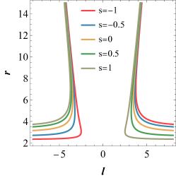
The the right panel of Fig. 3 shows the effect of spin on the circular stable or unstable branches for fixed . When , an ISCO exists for all values of within the range . As increases, the angular momentum of ISCO decreases. The trend of its variation with spin is consistent with the results in [36] where quantum effects are not considered.

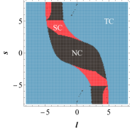
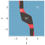
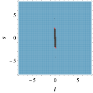
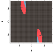
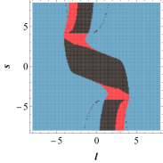
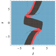
When obtaining the ISCO through (40) to (42), it is essential to verify whether the orbit is physical, i.e., whether it satisfies the timelike condition (32). In Fig. 4, for a fixed , in the parameter space, regions satisfying the timelike condition and allowing circular orbits are represented in blue, while regions possess spacelike circular orbits are shown in red. Black regions do not has circular orbits. By comparing the left three panels, it is evident that as increases, the parameter space for timelike circular orbits expands. The more pronounced the effects of loop quantum gravity, the smaller absolute value the angular momentum allowed for a timelike circular orbit. As a comparison, we can examine the branch. As illustrated in the Fig. 4 (d), it is evident that the blue region, representing timelike circular orbits, is small yet still present.
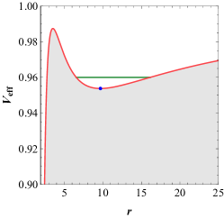
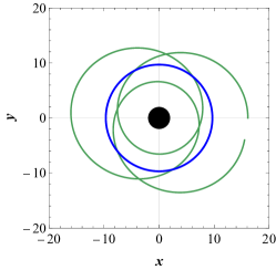
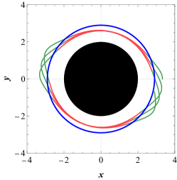
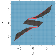
To more clearly illustrate the characteristics of timelike circular orbits, in Fig. 5, we present the rough shape of the orbit (see the three images in the second row, where the black circle represents the black hole, and the curves depict the particle trajectories) and the corresponding relation for a given parameter set of , , , and , where is the total energy for orbits colored in green and for blue. In panel (a) and (d), the stable circular orbit, marked in blue dot and curve, associated with the branch occurs at approximately with an energy of about . The green trajectory whose energy is approximately 0.960, is elliptical. When taking , and , the stable circular orbit is achieved at . However, the elliptical trajectory may exhibit spacelike regions at an energy of , which are marked in red in (e). The trajectory with both green and red segments is non-physical and needs to be excluded under the consideration of the timelike condition. The panel (c) and (f) has been mentioned above when we discuss Fig. 3. At this point, the angular velocity is vanishing the trajectory with energy hovers above the black hole, seeming to achieve a delicate balance between some repulsive force of loop quantum gravity and the classical gravitational attraction.
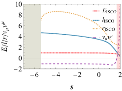
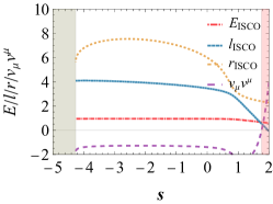
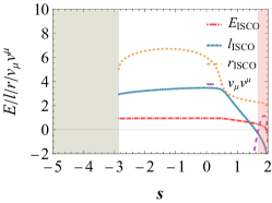
Finally we plot the ISCO parameter as the fuction of in Fig. 6 for different . The light pink region on the right of each panel represent spacelike region, where satisfy. The gray region does not contain an ISCO. The energy at the ISCO, , depicted by the red dash-dotted line remains relatively stable across varying values of for different . The angular momentum , shown in blue dashed lines, decreases as approaches zero and then drops more steeply for positive values of , meaning that the sign of spin would affect the orbital angular momentum for ISCO. The radius , plotted in orange dotted lines, initially rises with increasing , reaching a peak, and then declines as further increases. It goes through rapid change, meaning that distinct give quite different circular orbits.
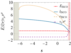
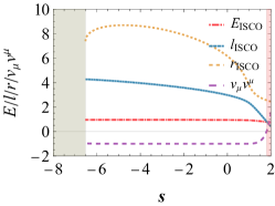
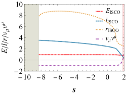
To clearly show the effect of LQG on the allowed spin of ISCO, we also numerically solved for the spin values corresponding to the left gray boundary and the right pink boundary for different values of , and recorded them in Table 1. The parameter , which denotes the boundary spin value where the timelike orbit intersects with the edge of spacelike orbit, gradually increases with the growth of . In contrast, , representing the minimum spin required for the ISCO orbit under a fixed loop quantum gravity-modified metric, does not exhibit a definitive trend in response to changes in . However, larger loop quantum gravity significantly gives larger allowable spin range for the ISCO. This influence could provide valuable insights in future observational experiments, such as gravitational wave detections, where the quantum aspects of gravity might be probed through phenomena associated with the ISCO.
| 0 | 1.652 | -6.15 |
| 1 | 1.706 | -6.16 |
| 2 | 1.798 | -6.52 |
| 3 | 1.814 | -8.27 |
IV The Motion of Spinning Particles in the solution 2 Spacetime
IV.1 Effective potential
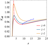
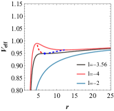
In this section, we apply a similar approach to investigate the effective potential and ISCO for the covariant gravity-corrected metric given by Eq. (4). We begin by examining the effective potential , as illustrated in Fig. 7. The overall trend of the effective potential is similar to that of (2). However, a notable difference appears in Fig. 7(b), where the effective potential diminishes as the loop quantum gravity effect strengthens, in contrast to the result from the first covariant solution. This implies that the two solutions are fundamentally different, and their respective parameters have opposite effects on the ISCO trajectory, such as the permissible spin range. Our subsequent research has also confirmed this point.
IV.2 ISCO
In Fig. 8, we plot the variation of these two extremal points in the plane for different values of or . As shown in the left panel of Fig. 3, larger value of may change the sign of the angular momentum of the turning point. A notable difference is observed in solution 2, where the ISCO remains present even when is significantly large, contrasting sharply with solution 1. Once is fixed, variations in spin consistently affect the turning point in the same way as solution 1: a higher spin results in a smaller ISCO angular momentum, as illustrated in the right panel.
After considering the timelike condition, we illustrate the allowed regions for stable circular orbits in the plane for both and in Fig. 9. The blue-shaded regions still represent the parameter ranges where stable, timelike circular orbits exist. For the branch, as increases from 4 to 16, we observe a relatively slight narrowing of the red and dark regions, representing spacetime circular orbits and no circular orbits respectively, indicating that the allowable parameter space for stable timelike circular orbits increases as the loop quantum gravity effects intensify. For branch, allowed region is quite small but still exist, and we find it getting larger as getting bigger.

Through the analysis above, we have finally plotted the variation of ISCO parameters as a function of spin in Fig. 10.
We also provide the numerical results for and under various values of in Table II. It can be observed that changes gradually with increasing , whereas grows rapidly due to the pronounced effects of loop quantum gravity. Specifically, under the conditions of solution 2, stronger quantum effects impose stricter constraints on the timelike ISCO, thereby reducing the permissible spin range. This stands in stark contrast to the result observed in solution 1.
| 0M | 1.652 | -6.15 |
| 2M | 1.692 | -5.38 |
| 4M | 1.761 | -4.26 |
| 6M | 1.762 | -3.45 |
| 8M | 1.687 | -2.86 |
V Conclusion and Discussion
In this paper, we have examined the dynamics of spinning particles in covariant loop quantum gravity black hole spacetimes, focusing on two effective metric solutions. Both of these metrics include a loop quantum characteristic parameter , and when it tends to zero, the spacetime background reduces to the Schwarzschild metric. Due to the spin-curvature force, the particle’s trajectory deviates from the geodesic, and its 4-momentum is no longer parallel to its 4-velocity. By employing the pole-dipole approximation, we derived the modified equations of motion and imposed timelike constraints to ensure physically meaningful solutions. Using the expression for the radial momentum, we introduced the effective potential to simplify the analysis of the motion. Based on the three conditions for the ISCO described by the effective potential, we derived the ISCO in the spacetime with loop quantum corrections and provided the corresponding parametric relationships. Our analysis of the effective potential revealed significant deviations from classical general relativity, particularly in the behavior of the Innermost Stable Circular Orbit (ISCO) and particle trajectories.
For the first effective metric, we found that the overall height and steepness of the effective potential increase with the loop quantum gravity parameter , which causes a shift in the radial position of circular orbits compared to the Schwarzschild spacetime, thereby further affecting the radial location of the ISCO. Additionally, we found that for a given particle spin, such as , if exceeds approximately 4.55, the entire spacetime no longer possesses an ISCO, a feature distinct from the purely classical spacetime background. This also leads to solutions where particles may hover above the black hole, and we have illustrated the corresponding trajectories in this paper. Furthermore, due to the timelike constraint, a larger imposes less stringent requirements on the spin of particles capable of forming an ISCO, which may provide guidance for observing quantum gravitational effects.
In contrast, the second effective metric displays a different behavior. The effective potential decreases and flattens as increases. Perhaps for this reason, the ISCO persists even when takes much larger values compared to solution 1. Moreover, larger values of impose stricter constraints on the allowable spin range for the ISCO, which is in stark contrast to the behavior observed in solution 1. This prompts us to consider that, although both metrics represent quantum corrections to gravity under the aim of preserving covariance, their effects on the behavior of orbiting particles, particularly the ISCO, may differ significantly. This suggests that the two metrics possess notable differences in their spacetime structures. Why the same covariance principle leads to such distinct structures is a question we will continue to explore.
Future studies could extend this analysis by exploring other black hole solutions, such as those with higher-dimensional spacetimes or alternative quantum gravity frameworks. Additionally, further investigation into the role of quantum effects in more realistic, rotating black hole spacetimes (Kerr or Kerr-Newman) may offer deeper insights into the interplay between spin and quantum geometry. Gravitational wave observations, such as those detected by LIGO, provide an exciting opportunity to test these predictions. Detecting deviations from classical predictions in the inspiral and merger phases of black hole binaries could offer a window into the quantum nature of gravity. Overall, our findings lay the groundwork for future studies to bridge the gap between quantum gravity and observational astrophysics, enhancing our understanding of black hole interiors and the quantum structure of spacetime.
Acknowledgements.
This work is supported by National Natural Science Foundation of China (NSFC) with Grants No.12275087.References
- [1] A. Papapetrou, “Spinning test-particles in general relativity. I,” Proc. R. Soc. A 209, 248–258 (1951).
- [2] B. P. Abbott et al. (LIGO Scientific Collaboration and Virgo Collaboration), “Observation of Gravitational Waves from a Binary Black Hole Merger,” Phys. Rev. Lett. 116, 061102 (2016).
- [3] B. P. Abbott et al. (LIGO Scientific Collaboration and Virgo Collaboration), “GW151226: Observation of Gravitational Waves from a 22-Solar-Mass Binary Black Hole Coalescence,” Phys. Rev. Lett. 116, 241103 (2016).
- [4] B. P. Abbott et al. (LIGO Scientific Collaboration and Virgo Collaboration), “GW170104: Observation of a 50-Solar-Mass Binary Black Hole Coalescence at Redshift 0.2,” Phys. Rev. Lett. 118, 221101 (2017).
- [5] B. P. Abbott et al. (LIGO Scientific Collaboration and Virgo Collaboration), “GW170814: A Three-Detector Observation of Gravitational Waves from a Binary Black Hole Coalescence,” Phys. Rev. Lett. 119, 141101 (2017).
- [6] B. P. Abbott et al. (LIGO Scientific Collaboration and Virgo Collaboration), “GW170817: Observation of Gravitational Waves from a Binary Neutron Star Inspiral,” Phys. Rev. Lett. 119, 161101 (2017).
- [7] B. P. Abbott et al. (LIGO Scientific Collaboration and Virgo Collaboration), “GWTC-1: A Gravitational-Wave Transient Catalog of Compact Binary Mergers Observed by LIGO and Virgo during the First and Second Observing Runs,” Phys. Rev. X 9, 031040 (2019).
- [8] B. P. Abbott et al. (LIGO Scientific Collaboration and Virgo Collaboration), “GWTC-2: Compact Binary Coalescences Observed by LIGO and Virgo during the First Half of the Third Observing Run,” Phys. Rev. X 11, 021053 (2021).
- [9] S. Suzuki and K. Maeda, “Gravitational waves from inspiraling compact binaries,” Phys. Rev. D 58, 023005 (1998).
- [10] M. Shibata, K. Taniguchi, and T. Nakamura, “Fully General Relativistic Simulations of Black Hole-Accretion Disk Systems,” Prog. Theor. Phys. Suppl. 128, 295 (1997).
- [11] J. L. Zdunik, P. Haensel, D. Gondek-Rosinska, and E. Gourgoulhon, “Non-rotating Neutron Stars with Quark Matter Cores,” Astron. Astrophys. 372, 535 (2001).
- [12] T. W. Baumgarte, “Neutron Star Merger Simulations with Relativistic Codes,” AIP Conf. Proc. 575, 176 (2001).
- [13] P. Grandclement, E. Gourgoulhon, and S. Bonazzola, “Binary neutron star systems: From post-Newtonian approximations to fully relativistic numerical models,” Phys. Rev. D 65, 044021 (2002).
- [14] M. A. Miller, P. Gressman, and W. M. Suen, “Magnetized Neutron Star Mergers in Full General Relativity,” Phys. Rev. D 69, 064026 (2004).
- [15] P. Marronetti, M. D. Duez, S. L. Shapiro, and T. W. Baumgarte, “Coupled quark-hadron equations of state in neutron star mergers,” Phys. Rev. Lett. 92, 141101 (2004).
- [16] D. Gondek-Rosinska, M. Bejger, T. Bulik, E. Gourgoulhon, P. Haensel, F. Limousin, and L. Zdunik, “Effects of quark matter on the neutron star inspiral,” Adv. Space Res. 39, 271 (2007).
- [17] M. Campanelli, C. O. Lousto, and Y. Zlochower, “Spin dynamics of black-hole binaries: Precession and merger,” Phys. Rev. D 73, 061501 (2006).
- [18] P. Shahrrear and S. B. Faruque, “Models of Rotating Black Holes in Higher Dimensions,” Int. J. Mod. Phys. D 16, 1863 (2007).
- [19] C. Cabanac, R. P. Fender, R. J. H. Dunn, and E. G. Koerding, “Ultraluminous X-ray Sources as Black Hole Binaries,” Mon. Not. R. Astron. Soc. 396, 1415 (2009).
- [20] A. Abdujabbarov and B. Ahmedov, “Electromagnetic radiation from relativistic charged particles in magnetized Kerr black hole,” Phys. Rev. D 81, 044022 (2010).
- [21] S. Hadar, B. Kol, E. Berti, and V. Cardoso, “Detecting gravitational waves from inspiraling neutron stars,” Phys. Rev. D 84, 047501 (2011).
- [22] S. Akcay, L. Barack, T. Damour, and N. Sago, “Radiation reaction on the ISCO of compact binaries,” Phys. Rev. D 86, 104041 (2012).
- [23] S. Hod, “Resonance frequencies of rapidly rotating Kerr black holes,” Phys. Rev. D 87, 024036 (2013).
- [24] C. Chakraborty, “The ISCO of spinning particles in Kerr spacetime: implications for accretion disk,” Eur. Phys. J. C 74, 2759 (2014).
- [25] S. Hod, “Quasi-normal modes of charged black holes,” Eur. Phys. J. C 74, 2840 (2014).
- [26] O. B. Zaslavskii, “Acceleration of particles near rotating black holes,” Eur. Phys. J. C 75, 403 (2015).
- [27] P. I. Jefremov, O. Yu. Tsupko, and G. S. Bisnovatyi-Kogan, “Motion of spinning particles in the Schwarzschild field: Circular orbits,” Phys. Rev. D 91, 124030 (2015).
- [28] M. Mathisson, “Neue Mechanik materieller Systeme,” Acta Phys. Pol. 6, 163 (1937).
- [29] G. Lukes-Gerakopoulos, E. Harms, S. Bernuzzi, and A. Nagar, “Spinning particles around a Schwarzschild black hole: Circular orbits,” Phys. Rev. D 96, 064051 (2017).
- [30] S. Motoyuki, M. Kei-ichi, S. Masaru, and M. Yasushi, “Gravitational waves from a spinning particle plunging into a Kerr black hole,” Phys. Rev. D 58, 064005 (1998).
- [31] Y. P. Zhang, S. W. Wei, W. D. Guo, T. T. Sui, and Y. X. Liu, “Innermost stable circular orbit of spinning particle in charged spinning black hole background,” Phys. Rev. D 97, 084056 (2018).
- [32] A. A. Deriglazov and W. G. Ramírez, “Mathisson-Papapetrou-Tulczyjew-Dixon equations in ultra-relativistic regime and gravimagnetic moment,” Int. J. Mod. Phys. D 26, 1750047 (2016).
- [33] A. A. Deriglazov and W. G. Ramírez, “Ultrarelativistic spinning particle and a rotating body in external fields,” Adv. High Energy Phys. 2016, 376016 (2016).
- [34] W. G. Ramírez and A. A. Deriglazov, “Relativistic effects due to gravimagnetic moment of a rotating body,” Phys. Rev. D 96, 124013 (2017).
- [35] A. A. Deriglazov and W. G. Ramírez, “Recent progress on the description of relativistic spin: Vector model of spinning particle and rotating body with gravimagnetic moment in general relativity,” Adv. Theor. Math. Phys. 2017, 7397159 (2017).
- [36] Y. P. Zhang, S. W. Wei, W. D. Guo, T. T. Sui, and Y. X. Liu, “Innermost stable circular orbit of spinning particle in charged spinning black hole background,” Phys. Rev. D 97, 084056 (2018).
- [37] K. Chen and S. W. Wei, “Motion of spinning particles around a polymer black hole in loop quantum gravity,” Phys. Rev. D 110, 024041 (2024).
- [38] P. I. Jefremov, O. Yu. Tsupko, and G. S. Bisnovatyi-Kogan, “Innermost stable circular orbits of spinning test particles in Schwarzschild and Kerr space-times,” Phys. Rev. D 91, 124030 (2015).
- [39] E. Corinaldesi and A. Papapetrou, “Spinning test-particles in general relativity. II.,” Proc. R. Soc. A 209, 259 (1951).
- [40] W. G. Dixon, “Dynamics of extended bodies in general relativity. I. Momentum and angular momentum,” Proc. R. Soc. A 314, 499 (1970).
- [41] S. A. Hojman, “Ph.D. thesis,” Princeton University, 1975.
- [42] R. Hojman and S. A. Hojman, “Spinning charged test particles in a Kerr-Newman background,” Phys. Rev. D 15, 2724 (1977).
- [43] S. A. Hojman and F. A. Asenjo, “Can gravitation accelerate neutrinos?,” Classical Quantum Gravity 30, 025008 (2013).
- [44] N. Zalaquett, S. A. Hojman, and F. A. Asenjo, “Spinning massive test particles in cosmological and general static spherically symmetric spacetimes,” Classical Quantum Gravity 31, 085011 (2014).
- [45] R. Uchupol, J. V. Sarah, and A. H. Scott, “Spinning particles in Schwarzschild spacetime: Revisiting the Mathisson-Papapetrou-Dixon equations,” Phys. Rev. D 94, 044008 (2016).
- [46] S. W. Hawking, “Breakdown of Predictability in Gravitational Collapse,” Phys. Rev. D 14, 2460 (1976).
- [47] D. N. Page, “Information in Black Hole Radiation,” Phys. Rev. Lett. 71, 3743 (1993).
- [48] D. N. Page, “Average entropy of a subsystem,” Phys. Rev. Lett. 71, 1291 (1993).
- [49] S. D. Mathur, “The Information paradox: A Pedagogical introduction,” Class. Quant. Grav. 26, 224001 (2009).
- [50] A. Almheiri, D. Marolf, J. Polchinski and J. Sully, “Black Holes: Complementarity or Firewalls?,” JHEP 02, 062 (2013). “Quantum black holes and complementarity,” JHEP 07, 150 (2014). “Firewalls and the black hole information paradox,” JHEP 11, 107 (2012).
- [51] A. Ashtekar, “New variables for classical and quantum gravity,” Phys. Rev. Lett. 57, 2244 (1986).
- [52] C. Rovelli and L. Smolin, “Loop Space Representation of Quantum General Relativity,” Nucl. Phys. B 331, 80 (1990).
- [53] A. Ashtekar, C. Rovelli, and L. Smolin, “Weaving a classical geometry with quantum threads,” Phys. Rev. Lett. 69, 237 (1992).
- [54] C. Rovelli and L. Smolin, “Discreteness of area and volume in quantum gravity,” Nucl. Phys. B 442, 593 (1995).
- [55] T. Thiemann, “Anomaly-free formulation of non-perturbative, four-dimensional Lorentzian quantum gravity,” Phys. Lett. B 380, 257 (1996).
- [56] C. Rovelli and L. Smolin, “Spin networks and quantum gravity,” Phys. Rev. D 52, 5743 (1995).
- [57] A. Ashtekar and J. Lewandowski, “Quantum theory of geometry I: Area operators,” Class. Quant. Grav. 14, A55-A82 (1997).
- [58] T. Thiemann, “Quantum spin dynamics (QSD),” Class. Quant. Grav. 15, 839 (1998).
- [59] F. Fazzini, “Effective Kerr geometry from loop quantum gravity,” [arXiv:2409.17099 [gr-qc]].
- [60] J. Kumar, S. U. Islam, and S. G. Ghosh, “Loop Quantum Gravity motivated multihorizon rotating black holes,” [arXiv:2209.13562 [gr-qc]].
- [61] F. Caravelli and L. Modesto, “Spinning Loop Black Holes,” Class. Quant. Grav. 27, 245022 (2010), [arXiv:1006.0232 [gr-qc]].
- [62] L. Modesto, “Phenomenological Loop Quantum Geometry of the Schwarzschild Black Hole,” Int. J. Theor. Phys. 49, 1649-1683 (2010), [arXiv:0807.0665 [gr-qc]].
- [63] Y. Liu, Z. Feng, and X. Zhang, “Solar system constraints of a polymer black hole in loop quantum gravity,” Phys. Rev. D 105, 084068 (2022).
- [64] J. Lin and X. Zhang, “Effective four-dimensional loop quantum black hole with a cosmological constant,” Phys. Rev. D 110, 026002 (2024)
- [65] Z. Shi, Y. Ma and X. Zhang, “Higher-dimensional quantum Oppenheimer-Snyder model,” [arXiv:2408.15821 [gr-qc]].
- [66] X. Zhang, “Loop Quantum Black Hole,” Universe 9, no.7, 313 (2023)
- [67] M. Bojowald, S. Brahma, Juan D. Reyes, Covariance in models of loop quantum gravity: Spherical symmetry, Phys. Rev. D 92, 045043 (2015).
- [68] C. Zhang, J. Lewandowski, Y. Ma and J. Yang, “Black Holes and Covariance in Effective Quantum Gravity,” [arXiv:2407.10168 [gr-qc]].
- [69] I. Husin Belfaqih, M. Bojowald, S. Brahma, E. I. Duque, Black holes in effective loop quantum gravity: Covariant holonomy modifications, arXiv:2407.12087
- [70] L. Cafaro and J. Lewandowski, “Status of Birkhoff’s theorem in polymerized semiclassical regime of Loop Quantum Gravity,” (2024), [arXiv:2403.01910 [gr-qc]].
- [71] G. Lukes-Gerakopoulos, J. Seyrich, and D. Kunst, “Investigating the effective potential of the Mathisson-Papapetrou-Dixon equations for a spinning particle in a Kerr spacetime,” Phys. Rev. D 90, 104019 (2014).
- [72] J. Ben Achour, S. Brahma, and A. Marciano, “Spherically symmetric sector of self dual Ashtekar gravity coupled to matter: Anomaly-free algebra of constraints with holonomy corrections,” Phys. Rev. D 96, 026002 (2017), [arXiv:1608.07314 [gr-qc]].
- [73] L. Cafaro and J. Lewandowski, “Status of Birkhoff’s theorem in polymerized semiclassical regime of Loop Quantum Gravity,” (2024), [arXiv:2403.01910 [gr-qc]].
- [74] S. W. Hawking and G. F. R. Ellis, The Large Scale Structure of Space-Time, Cambridge Monographs on Mathematical Physics (Cambridge University Press, 1973).
- [75] J. Münch, “Causal structure of a recent loop quantum gravity black hole collapse model,” Phys. Rev. D 104, 046019 (2021), [arXiv:2103.17112 [gr-qc]].
- [76] J. Lewandowski, Y. Ma, J. Yang, and C. Zhang, “Quantum Oppenheimer-Snyder and Swiss Cheese Models,” Phys. Rev. Lett. 130, 101501 (2023), [arXiv:2210.02253 [gr-qc]].
- [77] A. Ashtekar, J. Olmedo, and P. Singh, “Quantum extension of the Kruskal spacetime,” Phys. Rev. D 98, 126003 (2018), [arXiv:1806.02406 [gr-qc]].
- [78] A. Ashtekar, T. Pawlowski, and P. Singh, “Quantum Nature of the Big Bang: An Analytical and Numerical Investigation. I,” Phys. Rev. D 73, 124038 (2006), [arXiv:gr-qc/0604013].
- [79] A. Ashtekar, T. Pawlowski, and P. Singh, “Quantum Nature of the Big Bang: Improved dynamics,” Phys. Rev. D 74, 084003 (2006), [arXiv:gr-qc/0607039].
- [80] J. R. Oppenheimer and H. Snyder, “On Continued gravitational contraction,” Phys. Rev. 56, 455–459 (1939).