Anomalous dependence of sensitivity on observation time induced by time crystal order

Abstract

In this letter, we consider a composite atom-cavity system interacting with a ring resonator. In such a system, time crystal regime can be observed. We show that this regime can lead to a quadratic observation time dependence of the system’s sensitivity to perturbations due to ability to retain the memory of the atom’s initial state. Outside the time crystal regime, the system is not able to retain the memory of the atom’s initial state and the sensitivity scales linearly on the observation time. Our results open up a new way for implementation of discrete time crystals in sensing and metrology.

Recently, systems with spontaneously broken time translation symmetry and time crystals have attracted increasing interest. Originally, the concept of time crystals was proposed by F. Wilczek [1]. This concept based on the phenomenon of spontaneous breaking of time translation symmetry. Despite being criticized initially [2, 3, 4], the concept was extended to periodically driven Hamiltonian systems [5, 6, 7, 8]. The external periodic force generates a discrete time translation symmetry $H(t)=H(t+T)$ with respect to time period of external driving $T$ [7, 8]. Spontaneous breaking of time translation symmetry consists in the fact that there is a quantity in the system that changes with a multiple period of external driving $T^{\prime}=mT,m=2,3,...$ [7, 8]. There are a number of systems where is possible to observe discrete time crystals, for example, driven atom-cavity systems [9], systems with trapped ions [10], NV-center systems [11], open optomechanical systems [12] and NMR systems [13, 14].

Discrete time crystal systems and systems with spontaneously broken symmetries in general have intriguing and promising applications in quantum computation [15, 16] and in quantum metrology and sensing [17, 18, 19, 20, 21]. For example, time crystal-based quantum devices also demonstrate sensitivity scaling of particle number that exceeds the Heisenberg limit [21]. This fact opens up a new possible way of using time crystals in sensors.

In this letter, we consider a system consisting of a rotating ring resonator coupled with single-mode cavity, in which an active atom is placed. In such a system the spontaneous breaking of time translation symmetry can be observed [22]. We demonstrate that the influence of perturbations of system’s parameters, i.e. the sensitivity of the system, depends on an observation time as $T^{2}$ in the time crystal regime. On the other hand, outside the time crystal regime, the sensitivity demonstrates linear dependence on the observation time. This effect is explained by the fact that in the time crystal regime, the system is able to retain the memory of its initial atom’s state, which leads to a quadratic dependence of the sensitivity to perturbation magnitude on the observation time. Outside the time crystal regime, the system is not able to retain the memory of the initial state, so the dependence on the observation time becomes linear. This result can be useful for enhancing sensitivity of system with rotational-broken symmetry, e.g., optical gyroscopes.

We consider a system consisting of an active two-level atom placed into the single-mode cavity coupled with a ring resonator of length $L=2\pi R$. We consider the transition frequency of the atom and the frequency of the single-mode cavity both equal to $\omega_{0}$. In what follows, we consider $N$ modes whose frequencies lie close to ${\omega_{0}}$ and assume that ${\omega_{0}}/\delta\omega={j_{0}}$ is an integer number. In the system without perturbation, the ring resonator modes are divided into ”clockwise” and ”counterclockwise” modes, whose frequencies are given as $\omega_{j}^{\pm}=j\,\delta\omega$, where $\delta\omega=2\pi c/L$ is a step between the modes’ frequencies. When the system under consideration rotates with angular frequency ${\Omega_{rot}}$, the frequencies of ”clockwise” and ”counterclockwise” modes take the form $\omega_{j}^{\pm}=j\,\delta{\omega^{\pm}}\approx j\,\delta\omega\left({1\pm\varepsilon}\right)$, where $\delta{\omega^{\pm}}=\frac{{2\pi\left({c\pm{\Omega_{rot}}\cdot R}\right)}}{L}\approx\delta\omega\left({1\pm\frac{{{\Omega_{rot}}\cdot R}}{c}}\right)$ are steps between the modes’ frequencies for ”clockwise” and ”counterclockwise” and $\varepsilon={\Omega_{rot}}\cdot R/c<<1$. The shift in the mode frequencies caused by the rotation of the system can be considered as a perturbation.

We investigate the dynamics of the system for different values $\varepsilon$ and for different values of the coupling strength between the atom and the single-mode resonator. We use the following Hamiltonian for the system [23]:

$$\begin{array}[]{l}\hat{H}={\omega_{0}}\hat{\sigma}^{\dagger}{{\hat{\sigma}}}+{\omega_{0}}\hat{a}^{\dagger}{{\hat{a}}}+\Omega(\hat{a}{{\hat{\sigma}^{{\dagger}}}}+\hat{a}^{{\dagger}}{{\hat{\sigma}}})+\\ \sum\limits_{j=j_{0}-N/2}^{j_{0}+N/2}{{\omega_{j}^{+}}\hat{\alpha}_{j}^{\dagger}{{\hat{\alpha}}_{j}}}+\sum\limits_{j=j_{0}-N/2}^{j_{0}+N/2}{{g_{j}}(\hat{a}{{\hat{\alpha}}_{j}^{{\dagger}}}+\hat{a}^{{\dagger}}{{\hat{\alpha}}_{j}})}+\\ \sum\limits_{j=j_{0}-N/2}^{j_{0}+N/2}{{\omega_{j}^{-}}\hat{\beta}_{j}^{\dagger}{{\hat{\beta}}_{j}}}+\sum\limits_{j=j_{0}-N/2}^{j_{0}+N/2}{{g_{j}}(\hat{a}{{\hat{\beta}}_{j}^{{\dagger}}}+\hat{a}^{{\dagger}}{{\hat{\beta}}_{j}})}\end{array}$$ (1)

where $\hat{\sigma}$ and $\hat{\sigma}^{{\dagger}}$ are annihilation and creation operators of two-level atom that obey the fermionic commutation relation $\{\hat{\sigma},\hat{\sigma}^{{\dagger}}\}=1$. $\hat{a}$ and $\hat{a}^{{\dagger}}$ are annihilation and creation operators of the single-mode cavity. $\hat{\alpha}_{j}$, $\hat{\alpha}_{j}^{{\dagger}}$ and $\hat{\beta}_{j}$, $\hat{\beta}_{j}^{{\dagger}}$ are annihilation and creation operators of ”clockwise” and ”counterclockwise” modes of the ring resonator, respectively. The operators of the single-mode cavity and the ring resonator modes obey the bosonic commutation relations $[\hat{a},\hat{a}^{{\dagger}}]=1$, $[\hat{\alpha}_{i},\hat{\alpha}_{j}^{{\dagger}}]=\delta_{ij}$ and $[\hat{\beta}_{i},\hat{\beta}_{j}^{{\dagger}}]=\delta_{ij}$. $\Omega$ is the coupling strength between the single-mode cavity and the atom. We consider both groups of modes to interact with the single-mode cavity with the same coupling strength, i.e. $g_{j}=g$ for all $j$.

The dynamics of the system are determined by the time-dependent Schrödinger equation for a wave function $|\Psi(t)\rangle$. The system is assumed to have only one excitation quantum that can be in the atom, in the single-mode cavity, or in one of the ring resonator ”clockwise” and ”counterclockwise” modes. We look for the wave function in the following form [23]:

$$\begin{array}[]{l}|\Psi(t)\rangle=C_{\sigma}(t)|e,0,0,0\rangle+C_{a}(t)|g,1,0,0\rangle+\\ \sum\limits_{j=j_{0}-N/2}^{j_{0}+N/2}{C_{j}^{+}(t)|g,0,1_{j}^{+},0\rangle}+\sum\limits_{j=j_{0}-N/2}^{j_{0}+N/2}{C_{j}^{-}(t)|g,0,0,1_{j}^{-}\rangle}\end{array}$$ (2)

where $|e,0,0,0\rangle$, $|g,1,0,0\rangle$, $|g,0,1_{j}^{+},0\rangle$ and $|g,0,0,1_{j}^{-}\rangle$ are the states, in which the excitation quantum is in the atom, in the single-mode cavity, in one of the ring resonator ”clockwise” and ”counterclockwise” modes, respectively. $C_{\sigma}(t)$, $C_{a}(t)$, $C_{j}^{+}(t)$ and $C_{j}^{-}(t)$ are the amplitudes of probability of finding the excitation quantum in the atom, in the single-mode cavity, or in one of the ring resonator ”clockwise” and ”counterclockwise” modes, respectively.

We can obtain the closed system of equations for the probability amplitudes after substituting the wave function (2) into the Schrödinger equation with Hamiltonian (1):

$$\frac{{d{C_{\sigma}}}}{{dt}}=-i{\omega_{0}}{C_{\sigma}}-i\,\Omega{C_{a}}$$ (3)

$$\frac{{d{C_{a}}}}{{dt}}=-i{\omega_{0}}{C_{a}}-i\,\Omega{C_{\sigma}}-i\sum\limits_{j=j_{0}-N/2}^{j_{0}+N/2}{g{C_{j}^{+}}}-i\sum\limits_{j=j_{0}-N/2}^{j_{0}+N/2}{g{C_{j}^{-}}}$$ (4)

$$\frac{{d{C_{j}^{+}}}}{{dt}}=-i{\omega_{j}^{+}}{C_{j}^{+}}-ig{C_{a}}$$ (5)

$$\frac{{d{C_{j}^{-}}}}{{dt}}=-i{\omega_{j}^{-}}{C_{j}^{-}}-ig{C_{a}}$$ (6)

We also assume that at the initial moment of time, the excitation quantum is in the atom, i.e. $C_{\sigma}(0)=1$ and $C_{a}(0)=C_{j}^{+}(0)=C_{j}^{-}(0)=0,j=j_{0}-N/2,...,j_{0}+N/2$. In the following evolution the atom emits a photon into the ring resonator. The electromagnetic wave makes a complete bypass of the ring resonator in time $T_{R}=L/c=2\pi/{\delta\omega}$.

The system under consideration is in the regime of time crystal when the coupling strength is less than the critical coupling strength [22]. The critical coupling strength of the time crystal regime can be calculated in a similar way as presented in [22]. The time crystal regime begins to disrupt when the $\gamma^{\prime}T_{R}\thicksim 1$, where $\gamma^{\prime}$ is effective dissipation rate of the atom’s probability amplitude in the time crystal regime and $T_{R}$ is the time of one bypass of the ring resonator. $\gamma^{\prime}=\Omega^{2}/\gamma$, where $\Omega<<\gamma$ and $\gamma=\frac{2\pi g^{2}}{\delta\omega}$ is the atom’s probability amplitude dissipation rate that is calculated in Born-Markovian approximation [24, 25] with the elimination of the ring resonators’ degrees of freedom [22, 24, 25, 26]. Thus, the condition $\gamma^{\prime}T_{R}\thicksim 1$ can be written as $\Omega\thicksim g$. The value of the coupling strength $\Omega=\Omega_{TC}=g$ is the critical coupling strength of the time crystal regime.

The value of the effective dissipation rate $\gamma^{\prime}$ gives an estimation for the effective time of relaxation $T_{eff}\sim 1/{\gamma^{\prime}}$. However, in the time crystal regime the atom’s probability amplitude does not dissipate and oscillates near initial state in any observable time interval (see Fig 1 (a)). In opposite, outside the time crystal regime the atom’s probability amplitude completely dissipates in the time interval that is less then $T_{R}$ (Fig 1 (b)). This effect indicates the ability of the system to retain the memory of the atom’s state in the time crystal regime and its absence outside the time crystal regime.

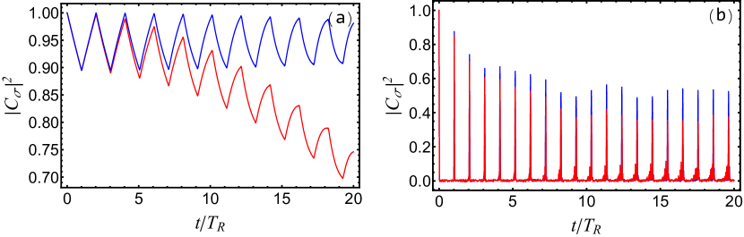
Figure 1: Dependence of the atom’s probability density $|C_{\sigma}(t)|^{2}$ on time in the case of zero perturbations $\varepsilon=0$ (blue solid line) and in the case of non-zero perturbation $\varepsilon=10^{-4}$ (red solid line) in the time crystal regime $\Omega=0.25\cdot\Omega_{TC}$ (a) and outside the time crystal regime $\Omega=8\cdot\Omega_{TC}$ (b). Here $T_{R}$ is the time of one bypass of the ring resonator. We consider $N=50$, $\delta\omega=4\cdot 10^{-3}\omega_{0}$, $g=6\cdot 10^{-3}\omega_{0}$.

The presence of perturbations leads to change in the system’s dynamics [Figure 1]. To characterize the influence of the perturbation, we calculate the relative difference between the time-averaged probability densities of the atom for zero and nonzero perturbation magnitudes. We determine a sensitivity of the system to the magnitude of perturbation as

$$S(T,\varepsilon,\Omega)=1-\int_{0}^{T}|C_{\sigma,\varepsilon\neq 0}|^{2}{dt}/\int_{0}^{T}|C_{\sigma,\varepsilon=0}|^{2}{dt}$$ (7)

where $T$ is an observation time. Figure 2 demonstrates the dependence of the value $S$ on the coupling strength $\Omega$ at fixed magnitude of perturbation $\varepsilon$ for different observation times $T=mT_{R}=m\frac{2\pi}{\delta\omega}$, where $m=5,10,15,20$. Figure 2 demonstrates that at $\Omega\sim\Omega_{TC}$ the sensitivity to the perturbation, $S$, increases noticeably more with the increasing of the observation time than in area $\Omega>>\Omega_{TC}$.

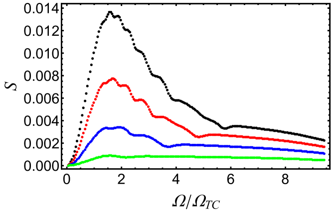
Figure 2: The dependence of the sensitivity $S$ on the coupling strength calculated over the observation time $T=5T_{R}$ (green dots), $T=10T_{R}$ (blue dots), $T=15T_{R}$ (red dots) and $T=20T_{R}$ (black dots). The magnitude of the perturbation is $\varepsilon=10^{-5}$. $N=50$, $\delta\omega=4\cdot 10^{-3}\omega_{0}$, $g=6\cdot 10^{-3}\omega_{0}$.

Our calculations show that with an increase in the observation time $T$ the value $S$ increases in power law $S\thicksim T^{\alpha}$. Figure 3 shows the dependence of the observation time power $\alpha$ on the coupling strength at fixed magnitude of perturbation $\varepsilon$. Our calculations show that for the coupling strengths corresponding to the time crystal regime, the degree is quadratic. Outside the time crystal regime, a transition area is observed, after which the dependence on the observation time becomes linear. However, it is important to note here that since the probability amplitude of the atom is always limited to one, the quadratic scaling of sensitivity on the observation time works only for limited time intervals. Then saturation sets in and the gain in sensitivity disappears. Our calculations demonstrate that the sensitivity in the area $\Omega\sim\Omega_{TC}$ becomes greater than in the area $\Omega>>\Omega_{TC}$, i.e., the quadratic time dependence exceeds the linear one, when the observation time is of order or greater than $10T_{R}$ (Fig. 2).

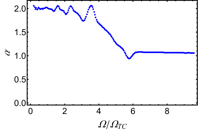
Figure 3: The dependence of the observation time exponent $\alpha$ of the sensitivity $S\thicksim T^{\alpha}$ on the coupling strength. The magnitude of the perturbation is $\varepsilon=10^{-5}$. $N=50$, $\delta\omega=4\cdot 10^{-3}\omega_{0}$, $g=6\cdot 10^{-3}\omega_{0}$.

Thus, in the time crystal regime, a quadratic dependence of the perturbation magnitude sensitivity on the observation time is observed. This is due to the fact that in the time crystal regime the atom’s state retains memory of its initial state. Indeed, as can be seen in Figure 1, in the time crystal regime, the state of the atom does not have sufficient time to completely dissipate. To understand how maintaining an atom’s state affects sensitivity, consider the interaction of the atom with the electromagnetic pulses it emits into multimode resonator. The radiation of the atom leads to the excitation of the electromagnetic pulses that propagate in clockwise and counterclockwise directions in the ring resonator. After a single pass through the ring resonator, the difference between the electromagnetic pulses emitted by the atom and propagating in opposite directions is equal to $\Delta\varphi={\varphi_{+}}-{\varphi_{-}}\sim{\Omega_{rot}}{T_{R}}$. Returning to the atom, the electromagnetic states act on the state of the atom. This action depends on the phase difference between the pulses. As a result, the state of the atom in the unperturbed system will differ from the state in the perturbed system by an amount that depends on ${\Omega_{rot}}{T_{R}}$ (i.e. $S\left({T={T_{R}}}\right)$is a function of ${\Omega_{rot}}{T_{R}}$). In the case where the difference between the perturbed and unperturbed systems is small, the linear approximation is applicable $S\left({{T_{R}}}\right)=A\,{\Omega_{rot}}{T_{R}}$, where $A$ is the proportionality coefficient. After the second pass through the resonator, the phase difference between the pulses becomes equal to $\Delta\varphi\sim 2{\Omega_{rot}}{T_{R}}$. In this case, the action of the pulses on the atom leads to an additional difference between the perturbed and unperturbed systems proportional to $2{\Omega_{rot}}{T_{R}}$. If the state of the atom does not have time to decay during the observation time, then the perturbations are summed up and the dependence of the sensitivity on time is determined by the expression $S\left(T\right)=A\,\int\limits_{0}^{T}{{\Omega_{rot}}{T_{R}}d{T_{R}}}\sim{T^{2}}$. Such a dependence takes place in the time crystal regime. If the state of the atom decays during the the time of one bypass of the ring resonator, then the difference in the states of the atom for the perturbed and unperturbed systems is determined only by the last action of the electromagnetic pulses. In this case, $S\left(T\right)\sim\Delta\varphi\sim T$. Such behavior is observed outside the time crystal regime.

Thus, in the time crystal regime, the current state of the atom is determined by the integral over all previous states. And therefore, the sensitivity is determined by contributions over the entire observation time ($S\left(T\right)\sim T^{2}$). On the contrary, outside the time crystal regime, the state of the atom completely dissipates during the one bypass of the ring resonator and so the sensitivity is determined by contributions only for the finite time interval ($S\left(T\right)\sim T$).

In conclusion, we consider the composite atom-cavity system interacting with the ring resonator. In this system there is a parameter range, in which the spontaneous breaking of time translation symmetry is possible. We demonstrate that the time crystal regime allows a quadratic increase in sensitivity with increasing observation time. This is due to the fact that in the time crystal regime the system is able to retain the memory of its initial atom’s state. At values of coupling strength greater than the critical coupling strength, when the time crystal regime is disrupted, the atom’s system begins to destroy significantly, losing memory of its initial state. Eventually, the dependence of sensitivity on the observation time becomes linear. The quadratic increase in sensitivity with increasing observation time opens up a new ways to create measuring devices, for example, such as optical gyroscopes.

Funding

Russian Science Foundation (No. 23-42-10010).

References

- Wilczek [2012] F. Wilczek, Quantum time crystals (2012).
- Bruno [2013] P. Bruno, Impossibility of spontaneously rotating time crystals: a no-go theorem, Phys. Rev. Lett. 111, 070402 (2013).
- Nozières [2013] P. Nozières, Time crystals: Can diamagnetic currents drive a charge density wave into rotation?, Europhysics Letters 103, 57008 (2013).
- Watanabe and Oshikawa [2015] H. Watanabe and M. Oshikawa, Absence of quantum time crystals, Phys. Rev. Lett. 114, 251603 (2015).
- Yao et al. [2017] N. Y. Yao, A. C. Potter, I.-D. Potirniche, and A. Vishwanath, Discrete time crystals: Rigidity, criticality, and realizations, Phys. Rev. Lett. 118, 030401 (2017).
- Gong et al. [2018] Z. Gong, R. Hamazaki, and M. Ueda, Discrete time-crystalline order in cavity and circuit qed systems, Phys. Rev. Lett. 120, 040404 (2018).
- Else et al. [2020] D. V. Else, C. Monroe, C. Nayak, and N. Y. Yao, Discrete time crystals, Annu. Rev. Condens. Matter Phys. 11, 467 (2020).
- Zaletel et al. [2023] M. P. Zaletel, M. Lukin, C. Monroe, C. Nayak, F. Wilczek, and N. Y. Yao, Colloquium: Quantum and classical discrete time crystals, Rev. Mod. Phys. 95, 031001 (2023).
- Keßler et al. [2021] H. Keßler, P. Kongkhambut, C. Georges, L. Mathey, J. G. Cosme, and A. Hemmerich, Observation of a dissipative time crystal, Phys. Rev. Lett. 127, 043602 (2021).
- Zhang et al. [2017] J. Zhang, P. W. Hess, A. Kyprianidis, P. Becker, A. Lee, J. Smith, G. Pagano, I.-D. Potirniche, A. C. Potter, A. Vishwanath, et al., Observation of a discrete time crystal, Nature 543, 217 (2017).
- Choi et al. [2017a] S. Choi, J. Choi, R. Landig, G. Kucsko, H. Zhou, J. Isoya, F. Jelezko, S. Onoda, H. Sumiya, V. Khemani, et al., Observation of discrete time-crystalline order in a disordered dipolar many-body system, Nature 543, 221 (2017a).
- Chen et al. [2024] D. Chen, Z. Peng, J. Li, S. Chesi, and Y. Wang, Discrete time crystal in an open optomechanical system, Phys. Rev. Res. 6, 013130 (2024).
- Rovny et al. [2018] J. Rovny, R. L. Blum, and S. E. Barrett, Observation of discrete-time-crystal signatures in an ordered dipolar many-body system, Phys. Rev. Lett. 120, 180603 (2018).
- Pal et al. [2018] S. Pal, N. Nishad, T. Mahesh, and G. Sreejith, Temporal order in periodically driven spins in star-shaped clusters, Phys. Rev. Lett. 120, 180602 (2018).
- Preskill [2018] J. Preskill, Quantum computing in the nisq era and beyond, Quantum 2, 79 (2018).
- Ippoliti et al. [2021] M. Ippoliti, K. Kechedzhi, R. Moessner, S. Sondhi, and V. Khemani, Many-body physics in the nisq era: Quantum programming a discrete time crystal, PRX Quantum 2, 030346 (2021).
- Frérot and Roscilde [2018] I. Frérot and T. Roscilde, Quantum critical metrology, Phys. Rev. Lett. 121, 020402 (2018).
- Bennett et al. [2020] R. Bennett, D. Steinbrecht, Y. Gorbachev, and S. Y. Buhmann, Symmetry breaking in a condensate of light and its use as a quantum sensor, Phys. Rev. Appl. 13, 044031 (2020).
- Choi et al. [2017b] S. Choi, N. Y. Yao, and M. D. Lukin, Quantum metrology based on strongly correlated matter, arXiv preprint arXiv:1801.00042 (2017b).
- Zhou et al. [2020] H. Zhou, J. Choi, S. Choi, R. Landig, A. M. Douglas, J. Isoya, F. Jelezko, S. Onoda, H. Sumiya, P. Cappellaro, et al., Quantum metrology with strongly interacting spin systems, Phys. Rev. X 10, 031003 (2020).
- Lyu et al. [2020] C. Lyu, S. Choudhury, C. Lv, Y. Yan, and Q. Zhou, Eternal discrete time crystal beating the heisenberg limit, Phys. Rev. Res. 2, 033070 (2020).
- Sergeev et al. [2024] T. T. Sergeev, A. A. Zyablovsky, E. S. Andrianov, and Y. E. Lozovik, Spontaneous breaking of time translation symmetry in a system without periodic external driving, Opt. Lett. 49, 4783 (2024).
- Scully and Zubairy [1999] M. O. Scully and M. S. Zubairy, Quantum optics (Cambridge University Press, 1999).
- Carmichael [2009] H. Carmichael, An open systems approach to quantum optics, Vol. 18 (Springer Science & Business Media, 2009).
- Gardiner and Zoeller [1991] C. Gardiner and P. Zoeller, Quantum noise (Springer-verlag, Berlin, 1991).
- Sergeev et al. [2022] T. T. Sergeev, I. V. Vovcenko, A. A. Zyablovsky, and E. S. Andrianov, Environment-assisted strong coupling regime, Quantum 6, 684 (2022).