The $D^{*}D\pi$ and $B^{*}B\pi$ couplings from Dyson-Schwinger equations framework

Abstract

Employing a unified Dyson-Schwinger/Bethe-Salpeter equations approach, we calculate the strong decay couplings $D^{*}D\pi$ and $B^{*}B\pi$ within the so-called impulse-approximation in the moving frame. The $B^{*}B\pi$ estimation is reported for the first time based on a Poincaré invariant computation of the associated Bethe-Salpeter amplitudes. Our predictions yield $g_{D^{*}D\pi}=16.22_{-0.01}^{+0.03}$ and $g_{B^{*}B\pi}=40.09_{-1.37}^{+1.51}$, along with corresponding static strong couplings of $\hat{g}_{D}=0.55_{-<0.01}^{+<0.01}$, $\hat{g}_{B}=0.50_{-0.02}^{+0.02}$. The numerical uncertainties arise from variations in the momentum partitioning parameter. Our results are consistent with recent experimental and lattice data.

1 Introduction

The investigation of the static and dynamical properties of the bound-states emerging from the strong interactions described by quantum chromodynamics (QCD), namely hadrons, is undoubtedly a fundamental topic in modern physics. Among these properties, the strong couplings of heavy-light pseudo-scalar and vector mesons with the pion turn out to be essential hadronic parameters for heavy flavor physics HFLAV:2022esi . The $D^{*}D\pi$ coupling ($g_{D^{*}D\pi}$) can be extracted from the total width of the $D^{*}$ meson by combining the branching fractions of the $D^{*}\rightarrow D\pi$ decays. On the contrary, the analogous $B^{*}B\pi$ case cannot be directly measured due to an insufficiency of phase-space for the $B^{*}\rightarrow B\pi$ decay to occur Flynn:2015xna . Its determination still remains important whatsoever Belyaev:1994zk ; Khodjamirian:2020mlb . For instance, because it approaches more closely to the heavy-quark limit than its $D-$meson counterpart, enabling a more precise identification of the so called static strong coupling $\hat{g}$ that characterizes the interaction of heavy-light mesons with the pion. The latter is vital within the context of heavy meson chiral perturbation theory Burdman:1992gh ; Wise:1992hn ; Yan:1992gz ; Flynn:2015xna .

In the past few decades, the determination of the $g_{H^{*}H\pi}$ couplings has attracted growing attention and various methods have been applied, for example, lattice QCD (lQCD) Flynn:2015xna ; Bernardoni:2014kla ; Can:2012tx ; Becirevic:2012pf ; Detmold:2012ge ; Detmold:2011bp , heavy quark effective theory (HQET) Cheung:2014cka , QCD sum rules (SR) Belyaev:1994zk ; Khodjamirian:2020mlb ; Duraes:2004uc ; Navarra:2001ju and the combined Dyson-Schwinger and Bethe-Salpeter equations framework (DSEs/BSEs) Jarecke:2002xd ; Mader:2011zf ; El-Bennich:2010uqs ; daSilveira:2022pte . From the diverse set of approaches, the latter stands out for its capability to provide a non-perturbative and Poincaré-covariant framework, capable of simultaneously capturing essential traits of QCD, such as confinement and dynamical chiral symmetry breaking (DCSB). Consequently, it has been exploited for over thirty years to scrutinize the different vacuum and in-medium facets of QCD as well as several hadron properties (see e.g. Refs. Roberts:1994dr ; Maris:1997hd ; Maris:1997tm ; Maris:1999nt ; Jarecke:2002xd ; El-Bennich:2010uqs ; Mader:2011zf ; Qin:2011dd ; Qin:2011xq ; Raya:2015gva ; Eichmann:2016yit ; Fischer:2018sdj ; Qin:2019oar ; Chen:2019otg ; Xu:2019ilh ; Serna:2020txe ; Xu:2020loz ; Xu:2021lxa ; Xu:2021mju ; Serna:2022yfp ; daSilveira:2022pte ; Li:2023zag ; Xu:2023vlt ; Xu:2023izo ; Xu:2024vkn ; Raya:2024ejx ; Xu:2024fun ; Shi:2024laj ).

The investigation of strong decays of light vector mesons, based upon a DSEs/BSEs treatment that yields Poincaré invariant Bethe-Salpeter amplitudes (BSAs), can be traced back to ref. Jarecke:2002xd , where the $\rho\to\pi\pi$, $\phi\to KK$ and $K^{*}\to K\pi$ decays were computed for the very first time within this approach. Results concerning the $\rho\pi\pi$ case were reanalyzed afterwards in ref. Mader:2011zf . Concurrent investigations that included $D$ and $B$-mesons were carried out in El-Bennich:2010uqs . These would constitute the latest explorations on the $B$-meson case under the DSEs/BSEs framework. Nonetheless, ref. El-Bennich:2010uqs utilizes a one-covariant model for the corresponding BSAs, which, while illustrative, compromises Poincaré invariance by truncating the structure of such Maris:1997hd ; Maris:1997tm . An updated account of these results, that leaves out the $B$-mesons, is provided in daSilveira:2022pte . Therein, a complete Dirac structure for the BSAs is considered, along with a truncation scheme similar in essence to the well-known rainbow-ladder (RL) approximation, which features a modified effective interaction to better capture the significant flavor asymmetry observed in heavy-light mesons Serna:2020txe ; Serna:2022yfp ; Chen:2019otg . While the $g_{D^{*}D\pi}$ estimation obtained in  daSilveira:2022pte aligns well with experimental expectations ParticleDataGroup:2022pth , such examination reveals some technical complexities in addressing heavy-light systems.

Recently, significant progress has been made in studying the properties and dynamics of heavy-light mesons using Poincaré-invariant Bethe-Salpeter amplitudes. This research encompasses various areas, including mass spectra, decay processes, distribution amplitudes, electromagnetic form factors, and generalized parton distributions Chen:2019otg ; Qin:2019oar ; Serna:2020txe ; Serna:2022yfp ; daSilveira:2022pte ; Xu:2024fun ; Shi:2024laj . In the present work, we build upon our previous work on the electromagnetic form factors of heavy-light mesons, Xu:2024fun , by extending the analysis to include the strong decay processes $D^{*}\rightarrow D\pi$ and $B^{*}\rightarrow B\pi$. Compared with previous DSEs/BSEs explorations, our BSAs are solved directly based upon a moving frame formulation of the corresponding BSEs, Bhagwat:2006pu , thus eliminating the uncertainties associated with fitting/extrapolation and reducing the error of the strong couplings. Notably, a prediction for the $B^{*}B\pi$ coupling is reported for the first time based on the Poincaré invariant determination of the BSAs. Our results are consistent with recent experimental extractions and available lattice data.

This manuscript is organized as follows: In section 2, we introduce the essential components for the computation of strong decays within the DSEs/BSEs framework. The obtained numerical results for the $D^{*}D\pi$ and $B^{*}B\pi$ couplings are presented in section 3. We also examine how contributions from the various Dirac structures characterizing the BSAs impact the overall results and provide a comparison with findings from other approaches. Finally, a brief summary is provided in section 4.

2 The strong coupling within DSEs/BSEs framework

2.1 The strong decays and the impulse approximation

The strong $H^{*}H\pi$ coupling, with $H=D,B$, can be defined by the on-shell matrix element Belyaev:1994zk ; El-Bennich:2010uqs

$$\left\langle H\left(P_{H}\right)\pi(P_{\pi})\mid H^{*}\left(P_{H^{*}},\lambda\right)\right\rangle=g_{H^{*}H\pi}\epsilon^{\lambda}\cdot P_{\pi},$$ (1)

where $\epsilon_{\mu}^{\lambda}$ is the polarization vector of the $H^{*}$ meson, and $P_{\pi}$, $P_{H}$, $P_{H^{*}}$ are the four-momenta of the pion, pseudo-scalar meson, and vector meson, respectively. We work in Euclidean space and these four-momenta satisfy the following on-shell conditions:

$$P_{\pi}^{2}=-M^{2}_{\pi};\ P_{H}^{2}=-M^{2}_{H};\ P_{H^{*}}^{2}=-M^{2}_{H^{*}}\,.$$ (2)

Within the widely used impulse approximation, the strong decay processes under examination can be evaluated from a triangle diagram that turns out to be fully characterized by the dressed quark propagators ($S$) and bound-state BSAs ($\Gamma_{H}$) as follows:

$$\tilde{\Lambda}_{\mu}=N_{c}\text{Tr}\int^{\Lambda}\frac{d^{4}\tilde{k}}{(2\pi)^{4}}S^{\bar{f}}\left(k_{p}\right)\Gamma_{H}^{(\text{out})}\left(k_{p};k_{+}\right)S^{g}\left(k_{+}\right)\Gamma_{\mu,H^{*}}^{\text{(in)}}\left(k_{+};k_{-}\right)S^{g}\left(k_{-}\right)\Gamma_{\pi}^{(\text{out})}\left(k_{-};k_{p}\right),$$ (3)

with $\epsilon^{\lambda}\cdot\tilde{\Lambda}=g_{H^{*}H\pi}\epsilon^{\lambda}\cdot P_{\pi}$. Here Tr stands for a trace over Dirac indices, $N_{c}=3$, and $\Lambda$ represents a regularization scale. In figure 1, a more intuitive pictorial representation of the above mathematical expression is shown. The computation of the components entering eq. (3) within the present DSEs/BSEs framework shall be detailed afterwards.

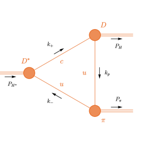
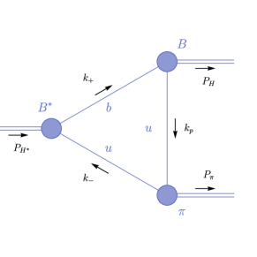
Figure 1: Left panel: $D^{*}\rightarrow D\pi$; right panel: $B^{*}\rightarrow B\pi$. The solid lines represent the dressed-quark propagator, the shaded circles denote the meson’s BSAs, and the black arrows indicate the direction of momentum. We work in the $\mathrm{SU}(2)$ isospin limit, hence $u=d$ quark.

What remains now is to define the kinematics to be adopted in eq. (3). For the momenta of quarks and mesons, we further define

$$P_{\pi} =-\tilde{P}+(1-\alpha)\tilde{Q},\ P_{H}=\tilde{P}+\alpha\tilde{Q},\ P_{H^{*}}=\tilde{Q};$$ (4a)

$$k_{+} =\tilde{k}+\alpha\tilde{Q},\ k_{-}=\tilde{k}-(1-\alpha)\tilde{Q},\ k_{p}=\tilde{k}-\tilde{P},$$ (4b)

where $\alpha$ is a momentum partitioning parameter associated to the $H^{*}$ meson, $\tilde{k}$ represents the integral momentum, and

$$\tilde{Q} =(0,0,0,1)|\tilde{Q}|,\ |\tilde{Q}|=iM_{H^{*}};$$ (5a)

$$\tilde{P} =(0,0,\sqrt{1-z^{2}},z)|\tilde{P}|,\ |\tilde{P}|=i\sqrt{M_{H}^{2}-\alpha\left((1-\alpha)M_{H^{*}}^{2}-M_{\pi}^{2}+M_{H}^{2}\right)}\,,$$ (5b)

with

$$z=\frac{(1-2\alpha)M_{H^{*}}^{2}-M_{\pi}^{2}+M_{H}^{2}}{2M_{H^{*}}\sqrt{M_{H}^{2}-\alpha\left((1-\alpha)M_{H^{*}}^{2}-M_{\pi}^{2}+M_{H}^{2}\right)}}\,.$$ (5c)

Plainly, $\tilde{Q}$ is the total momentum of the system, i.e.:

$$\tilde{Q}=P_{H^{*}}=P_{H}+P_{\pi}\,.$$ (6)

In the case of $M_{H}=M_{\pi},\ \alpha=1/2$, $\tilde{P}$ reduces to the relative momentum between the outgoing particles, namely:

$$\left.\tilde{P}\right|_{M_{H}=M_{\pi},\ \alpha=1/2}=\frac{P_{H}-P_{\pi}}{2}=(0,0,\kappa,0),\ \kappa^{2}=\frac{M_{H^{*}}^{2}}{4}-M_{\pi}^{2}\,,$$ (7)

which is consistent with the formulation employed in previous works for the calculation of the $\rho\rightarrow\pi\pi$ decay, as well as pseudo-scalar and vector meson electromagnetic form factors Mader:2011zf ; Jarecke:2002xd ; Xu:2024fun ; Xu:2024vkn ; Xu:2019ilh . We now proceed to discuss the evaluation of eq. (3), which, as mentioned above, follows directly from the prior computation of propagators and BSAs. We will see that the result for $g_{H^{*}H\pi}$ turns out to be independent of the choice of the momentum partitioning parameter due to the intrinsic Poincaré invariance of the DSEs/BSEs framework.

2.2 Quark propagators from DSEs

On general grounds, the dressed-quark propagators entering eq. (3) are expressed in terms of two Dirac structures as

$$S^{-1}(k)=i\gamma\cdot p\,A(k^{2})+B(k^{2})\,,$$ (8)

where $A(k^{2})$ and $B(k^{2})$ are scalar functions to be determined. Under the rainbow-ladder (RL) approximation, the quark propagator satisfies the following gap equation:

$$S^{-1}(k)=Z_{2}i\gamma\cdot k+Z_{4}m+Z_{1}\int^{\Lambda}\frac{d^{4}q}{(2\pi)^{4}}g^{2}D_{\alpha\beta}(l)\frac{\lambda^{a}}{2}\gamma_{\alpha}S(q)\frac{\lambda^{a}}{2}\gamma_{\beta}\,,$$ (9)

where $l=k-q$, $m$ is current-quark mass, and $Z_{1,2,4}$ are the renormalization constants. In this work we employ a mass-independent momentum-subtraction renormalization scheme, setting the renormalization scale at $\zeta=19$ GeV Chang:2008ec ; Xu:2021mju ; Xu:2024fun . In conjunction with the tree-level like vertex $\gamma_{\beta}$, which characterizes the RL truncation, we will adopt the following form for the gluon propagator:

$$Z_{1}g^{2}D_{\mu\nu}(l)=Z_{2}^{2}\mathcal{G}\left(l^{2}\right)\mathcal{P}_{\mu\nu}^{T}(l)=\mathcal{D}_{\text{eff}}\,,$$ (10)

where $\mathcal{P}_{\mu\nu}^{T}(l)=\delta_{\mu\nu}-{l_{\mu}l_{\nu}}/l^{2}$ is the standard transverse projection operator and, for the effective interaction, we employ the well-known Qin-Chang model Qin:2011dd ; Qin:2011xq :

$$\frac{\mathcal{G}(l^{2})}{l^{2}}=\mathcal{G}^{\text{IR}}(l^{2})+\frac{8\pi^{2}\gamma_{m}\mathcal{F}(l^{2})}{\ln[\tau+(1+l^{2}/\Lambda^{2}_{\text{QCD}})^{2}]},\ \mathcal{G}^{\text{IR}}(l^{2})=D\frac{8\pi^{2}}{\omega^{4}}e^{-l^{2}/\omega^{2}}\,.$$ (11)

The pieces entering the ultraviolet-dominating contribution are defined as follows: $\mathcal{F}(l^{2})=\{1-\exp[(-l^{2}/(4m_{t}^{2})]\}/l^{2}$, $m_{t}=0.5$ GeV, $\tau=e^{2}-1$, $\Lambda_{\text{QCD}}=0.234$ GeV, $\gamma_{m}=12/25$ Xu:2021mju . For the infrared component, in line with refs. Xu:2024fun ; Shi:2024laj we choose $(D\omega)_{u/d}=(0.82\ \text{GeV})^{3}$, $(D\omega)_{c}=(0.66\ \text{GeV})^{3}$, $(D\omega)_{b}=(0.48\ \text{GeV})^{3}$, with $\omega_{u/d}=0.5$ GeV, $\omega_{c,b}=0.8$ GeV. More details concerning eqs. (9-11) are found through Refs. Roberts:1994dr ; Maris:2003vk ; Maris:1997tm ; Qin:2011dd ; Maris:1999nt .

It is worth stressing that, in solving the bound-state problem, eq. (9) usually needs to be evaluated in the complex plane to ensure the relative momentum $l$ in the interaction model is real, Fischer:2005en ; Rojas:2014aka . Notably, $k^{2}$ is constrained by a parabola (see figure 2, gray region)

$$\text{Re}(k^{2})\geq-\Theta^{2}+\frac{\text{Im}^{2}(k^{2})}{4\Theta^{2}},$$ (12)

where $(-{\Theta}^{2},0)$ is the vertex of parabola. Once the quark propagator on this region is determined, its values at any interior point of the contour can be directly obtained using the Cauchy integral theorem Sanchis-Alepuz:2017jjd . However, poles in the complex plane compromise the applicability of this technique: they cannot be enclosed by the integration contour. For quarks of different flavors, the positions of the singularities vary Windisch:2016iud , so the maximum value adopted by the vertex also differs. In this work, we obtain $\Theta_{u}=0.56$ GeV, $\Theta_{c}=1.63$ GeV, $\Theta_{b}=4.8$ GeV.

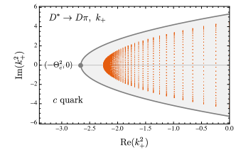
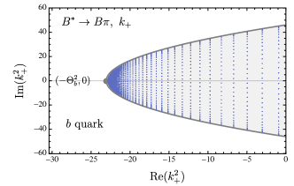
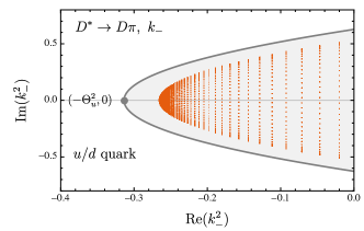
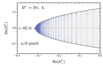
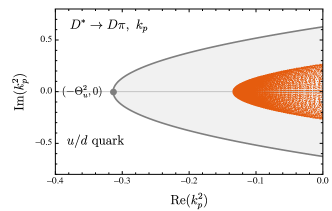
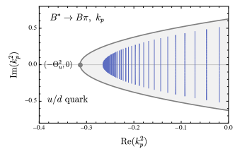
Figure 2: Required evaluation domain for the quark propagator. Colored points represent the actual required values of $k_{-}^{2}$, $k_{+}^{2}$, and $k_{p}^{2}$ when their real parts are less than zero, under the best $\alpha$. The gray area represents the region that is computable.

With the above on mind, note that the integral momentum $\tilde{k}$ in eq. (3) can be conveniently written as

$$\tilde{k}=(0,\sin\iota\sin\theta,\cos\iota\sin\theta,\cos\theta)|\tilde{k}|\,,$$ (13)

and, accordingly,

$$\text{Re}(k^{2}_{+}) =-\alpha^{2}M_{H^{*}}^{2}+\frac{\text{Im}^{2}(k^{2}_{+})\sec^{2}\theta}{4M_{H^{*}}^{2}\alpha^{2}},\ \theta\in[0,\pi]\,,$$ (14a)

$$\text{Re}(k^{2}_{-}) =-(1-\alpha)^{2}M_{H^{*}}^{2}+\frac{\text{Im}^{2}(k^{2}_{-})\sec^{2}\theta}{4M_{H^{*}}^{2}(1-\alpha)^{2}},\ \theta\in[0,\pi]\,.$$ (14b)

The resemblance between eq. (12) and eq. (14) is readily noticeable; in the latter case, this corresponds to making the association with the rest frame of the $H^{*}$ meson. Although the physical observables do not depend on $\alpha$, in the actual calculation, the selection of $\alpha$ should ensure that $k_{+}^{2}$ and $k_{-}^{2}$ remain within a computable region

$$\alpha^{2}M_{H^{*}}^{2}<\Theta^{2},\ (1-\alpha^{2})M_{H^{*}}^{2}<\Theta^{2},$$ (15)

such that

$$1-\Theta_{\bar{g}}/M_{H^{*}}<\alpha<\Theta_{f}/M_{H^{*}}\,.$$ (16)

Consequently, the best value of $\alpha$ can be defined as $\Theta_{f}/(\Theta_{f}+\Theta_{\bar{g}})$, which corresponds to the maximum computable mass $\Theta_{f}+\Theta_{\bar{g}}$ in the calculation of meson mass spectra Rojas:2014aka ; Xu:2024fun .

As for $k_{p}^{2}$ concerns, under the current notation, it cannot be expressed in a simple form similar to eq. (14). Nevertheless, numerical results show that $k_{p}^{2}$ remains within the computable region in the calculations of $D^{*}\rightarrow D\pi$ and $B^{*}\rightarrow B\pi$. Figure 2 displays the specific values required for $k_{-}^{2}$, $k_{+}^{2}$, and $k_{p}^{2}$ when their real parts are negative, given the best choice of $\alpha$.

2.3 Meson’s BSAs from BSEs

The next components entering eq. (3) are the corresponding meson’s BSAs. Generically, those satisfy the following homogeneous BSEs

$$\Gamma^{f\bar{g}}_{H}\left(k^{\prime}_{+},k^{\prime}_{-}\right)=\int^{\Lambda}\frac{d^{4}q}{(2\pi)^{4}}K^{f\bar{g}}(q,k;P)S^{f}\left(q_{+}\right)\Gamma^{f\bar{g}}_{H}\left(q_{+},q_{-}\right)S^{g}\left(q_{-}\right),$$ (17)

with $f$ and $g$ labeling the quark and antiquark flavors, and $K^{f\bar{g}}$ being the two-body interaction kernel. This shall be discussed afterwards. Denoting $P$ as the meson’s total momentum, the relative momentum between the valence quark and antiquark might be expressed as $q_{+}=q+\alpha^{\prime}P$, $q_{-}=q-(1-\alpha^{\prime})P$, with $\alpha^{\prime}\in[0,1]$ once again defining momentum partitioning parameter. Moreover, as mentioned below eq. (14), the current formulation can be interpreted as the rest frame of the $H^{*}$ meson, therefore $\alpha^{\prime}_{H^{*}}=\alpha$ and should fulfill the constraint in eq. (16). As for the $H$ meson and pion, since the momenta of the quark and antiquark external legs have already been fixed, the choice of $\alpha^{\prime}$ is inconsequential. Thus, once eq. (17) is solved within the coordinate system specified in eq. (5), the resulting BSAs can be directly used as input into eq. (3), eliminating the need to know the amplitudes outside the domain in which they were obtained.

Having specified the kinematics, let us now discuss the tensor structure of the BSAs. These have a general decomposition in terms of Dirac covariants as follows:

$$\Gamma\left(k^{\prime}_{+},k^{\prime}_{-}\right)=\sum_{i=1}^{N}\tau_{i}(k,P)F_{i}(k,P)\,,$$ (18)

where $\tau_{i}(k,P)$ are the basis tensors and $F_{i}(k,P)$ the associated scalar functions. For the pseudo-scalar mesons we choose Qin:2011xq :

$$\tau_{0^{-}}^{1} =i\gamma_{5}, \tau_{0^{-}}^{3}=\gamma_{5}\gamma\cdot kk\cdot P,$$

$$\tau_{0^{-}}^{2} =\gamma_{5}\gamma\cdot P, \tau_{0^{-}}^{4}=\gamma_{5}\sigma_{\mu\nu}k_{\mu}P_{\nu}\,,$$ (19a)

and, for their vector meson counterparts,

$$\tau_{1^{-}}^{1}=i\gamma_{\mu}^{T}, \tau_{1^{-}}^{5}=k_{\mu}^{T},$$

$$\tau_{1^{-}}^{2}=i\left[3k_{\mu}^{T}\gamma\cdot k^{T}-\gamma_{\mu}^{T}k^{T}\cdot k^{T}\right], \tau_{1^{-}}^{6}=k\cdot P\left[\gamma_{\mu}^{T}\gamma^{T}\cdot k-\gamma\cdot k^{T}\gamma_{\mu}^{T}\right],$$

$$\tau_{1^{-}}^{3}=ik_{\mu}^{T}k\cdot P\gamma\cdot P, \tau_{1^{-}}^{7}=\left(k^{T}\right)^{2}\left(\gamma_{\mu}^{T}\gamma\cdot P-\gamma\cdot P\gamma_{\mu}^{T}\right)-2k_{\mu}^{T}\gamma\cdot k^{T}\gamma\cdot P,$$

$$\tau_{1^{-}}^{4}=i\left[\gamma_{\mu}^{T}\gamma\cdot P\gamma\cdot k^{T}+k_{\mu}^{T}\gamma\cdot P\right], \tau_{1^{-}}^{8}=k_{\mu}^{T}\gamma\cdot k^{T}\gamma\cdot P,$$ (19b)

with $V_{\mu}^{T}=V_{\mu}-P_{\mu}(V\cdot P)/P^{2}$. Note that if the complete structure of the BSAs is not retained, the Poincaré invariance, a feature of the direct application of DSEs/BSEs to the calculation of hadron properties, would be compromised El-Bennich:2010uqs ; Maris:1997tm .

The final piece completing the BSE, eq. (17), is the two-body interaction kernel $K^{f\bar{g}}$. In the standard RL approximation, the interaction kernel is given by Xu:2021mju :

$$K^{f\bar{g}}(q,k;P)=\tilde{\mathcal{D}}^{f\bar{g}}_{\text{eff}}\frac{\lambda^{a}}{2}\gamma_{\alpha}\otimes\frac{\lambda^{a}}{2}\gamma_{\beta},\ \tilde{\mathcal{D}}^{f\bar{g}}_{\text{eff}}=\mathcal{D}^{f}_{\text{eff}},$$ (20)

where $\mathcal{D}^{f}_{\text{eff}}$, defined in eq. (10), describes the strength of interaction and decreases as the mass of quark increases because the quark dressing effects become suppressed Sultan:2018tet ; Serna:2017nlr ; Qin:2019oar . In combination with the one-body kernel described in the previous section, eq. (20) guarantees the axial-vector Ward-Takahashi identity (AV-WTI) is fulfilled, which ensures a massless pion in the chiral limit Munczek:1994zz . From a numerical perspective, the degree of preservation can be further tested by assessing the commensurateness between the expected and obtained results for the generalized Gell-Mann-Oakes-Renner (GMOR) relation Rojas:2014aka ; Chen:2019otg :

$$f_{0^{-}}M_{0^{-}}=\left(m_{f}+m_{g}\right)\rho_{0^{-}}\,.$$ (21)

Clearly, in the above expression, $M_{0^{-}}$ corresponds to the pseudo-scalar meson’s mass, while the quantity $\rho_{0^{-}}$ is defined as follows

$$\rho_{0^{-}}=Z_{4}N_{c}\text{Tr}\int^{\Lambda}\frac{d^{4}k}{(2\pi)^{4}}\gamma_{5}S^{f}\left(k_{+}\right)\Gamma_{0^{-}}^{f\bar{g}}(k_{+},k_{-})S^{\bar{g}}\left(k_{-}\right)\,;$$ (22)

and $f_{0^{-}}$ denotes the pseudo-scalar meson leptonic decay constant. Having properly normalized the BSAs Qin:2011xq , the decay constants related to the pseudo-scalar and the vector can be obtained from the following expressions:

$$f_{0-}P_{\mu} =Z_{2}N_{c}\text{Tr}\int^{\Lambda}\frac{d^{4}k}{(2\pi)^{4}}\gamma_{5}\gamma_{\mu}S^{f}\left(k_{+}\right)\Gamma_{0^{-}}^{fg}(k_{+},k_{-})S^{g}\left(k_{-}\right),$$ (23)

$$f_{1^{-}}M_{1^{-}} =Z_{2}N_{c}\text{Tr}\int^{\Lambda}\frac{d^{4}k}{(2\pi)^{4}}\gamma_{\mu}S^{f}\left(k_{+}\right)\Gamma_{1^{-}}^{\mu,fg}(k_{+},k_{-})S^{g}\left(k_{-}\right)\,.$$ (24)

Meson	Mass [GeV]				Leptonic decay constant [GeV]
	Expt.	lQCD	Rest frame	Moving frame	Expt.	lQCD	Rest frame	Moving frame
$\pi$	0.138(1)	-	0.135	0.135	0.092(1)	0.093(1)	0.095	0.095
$D$	1.868(1)	1.868(3)	1.868†	1.868	0.144(4)	0.150(4)	0.140	0.140
$D^{*}$	2.009(1)	2.013(14)	2.017	2.017	-	0.158(6)	0.160	0.160
$B$	5.279(1)	5.283(8)	5.279†	5.279	0.133(18)	0.134(1)	0.123	0.123
$B^{*}$	5.325(1)	5.321(8)	5.334	5.334	-	0.131(5)	0.126	0.126

Table 1: The produced masses and leptonic decay constants. Current quark masses are set as $m_{u,c,b}^{\xi=19\ \text{GeV}}=0.0033\ \text{GeV},0.854\ \text{GeV},3.682\ \text{GeV}$ Xu:2024fun and the script ^† denotes the fitting values from weight factor (see eq. (25)). Here we work in the isospin-symmetric limit $m_{u}=m_{d}$. For comparison, we collect both experimental values and lQCD’s results ParticleDataGroup:2022pth ; Dowdall:2012ab ; Cichy:2016bci ; Lubicz:2017asp ; Bazavov:2017lyh .

Over the past thirty years, the RL kernel has been widely used in flavor symmetric/slightly asymmetric systems such as $u\bar{d}$, $u\bar{s}$, $c\bar{c}$ (e.g. Qin:2011dd ; Ding:2015rkn ). However, for heavy-light systems, it is difficult to be applied because of the insufficiency of the RL truncation to properly capture the marked flavor-asymmetry. A proven and rapidly developing approach involves using modified RL schemes that adjust the BSE’s effective interaction to account for flavor asymmetry. This has allowed investigation of several aspects of heavy-light systems, ranging from mass spectra and decay constants, to electromagnetic form factors and many other quantities defined on the light-front Chen:2019otg ; Qin:2019oar ; Serna:2020txe ; Serna:2022yfp ; daSilveira:2022pte ; Xu:2024fun ; Shi:2024laj . In this work, we adopt the so-called weight-RL approximation, which arithmetically averages the RL kernels for different flavors as follows Qin:2019oar ; Xu:2024fun ; Shi:2024laj :

$$\tilde{\mathcal{D}}^{f\bar{g}}_{\text{eff}}=\eta\mathcal{D}^{f}_{\text{eff}}+(1-\eta)\mathcal{D}^{\bar{g}}_{\text{eff}}\,.$$ (25)

Here $\eta$ acts as a weighting factor, controlling the relative strength between the flavor-separated kernels. In the case of flavor-symmetric mesons, eq. (25) reduces to the RL kernel, hence maintaining the masslessness of the pion in the chiral limit and its Goldstone boson nature. For flavor-asymmetric systems, the effect of weight factor has been discussed in ref. Qin:2019oar , in which case it arises naturally from considering certain limits of a more elaborate truncation. In this case, $\eta$ is directly determined from the mass of the pseudo-scalar. This enables us to preserve the simplicities of the RL truncation but better capture the properties of the heavy-light mesons Xu:2024fun ; Shi:2024laj . After the proper determination of the weighting factor $\eta$, the leptonic decay constant of the $D,\ B$ mesons, as well as the mass and leptonic decay constant of the vector counterparts $D^{*},\ B^{*}$, emerge as genuine predictions. As can be seen from table 1, the resulting values are notably on par with experiment and other phenomenological determinations. Furthermore, an assessment through eq. (21), indicates a degree of AV-WTI preservation at the level of $\sim 97\%$.

It is worth noting that, under a strict heavy-light kernel, once the flavor-dependence of interaction is determined in gap equation, fitting for heavy-light mesons is not required. Therefore, the introduction weighting factor in this kernel ansatz should be considered as a cost of calculating heavy-light mesons in the RL-like framework, to remedy the effects of flavor asymmetry in BSEs. The theoretical exploration for flavor dependence within strict beyond-RL kernels is still ongoing and remains highly challenging Ivanov:1998ms ; Rojas:2014aka ; Gomez-Rocha:2016cji ; daSilveira:2022pte ; Chen:2019otg ; Qin:2020jig .

3 Numerical results and discussion

With all the above in hand, the strong coupling can be directly calculated based on eq. (3). Due to Poincaré invariance, $g_{H^{*}H}$ is in principle independent of the choice of $\alpha$ defined in eq. (4). However, as previously noted, in numerical computations, the value of $\alpha$ must be strictly constrained by eq. (16) due to the quark propagator’s domain of computability, which is influenced by its singularities in the complex plane. Consequently, by varying $\alpha$, we can assess the precision of our results and estimate the associated error.

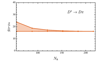
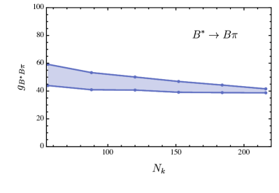
Figure 3: This figure shows that the uncertainty in $g_{H^{*}H\pi}$, caused by variations in the momentum partitioning parameter $\alpha$, progressively decreases as the accuracy of numerical integration improves. Here $N_{k}$ is the number of radial points of Gaussian numerical integration.

In figure 3, we present the numerical error resulting from variations in the momentum partitioning parameter $\alpha$. As the number of Gaussian quadrature points in the numerical integration increases, the obtained results become more precise. However, when compared to the rest frame, the memory requirements for solving the BSEs in a moving frame typically increase by two orders of magnitude ($\sim$ TB). While some relevant optimizations can be applied (see appendix A), the number of Gaussian integration points is still limited. So, after balancing our computational resources and precision, we report the final result as

$$g_{D^{*}D\pi}=16.22_{-0.01}^{+0.03},\ g_{B^{*}B\pi}=40.09_{-1.37}^{+1.51}\,.$$ (26)

It is well-established that the vector mesons BSAs are composed of eight independent Dirac structures (see eq. (19)), among which $\tau^{1}_{1^{-}}$ is usually considered the dominant term. Due to the relatively large number of Dirac covariants, it is worth analyzing the effects of including or neglecting different basis terms. For this purpose, table 2 provides a breakdown of the contributions from different vector BSAs to $g_{H^{*}H\pi}$, while a complementary visual representation of such is shown in figure 4.

$g_{D^{*}D\pi}$				$g_{B^{*}B\pi}$
$\tau^{1}_{D^{*}},\tau^{1}_{D}$	$29.94_{-0.01}^{+0.05}$	$\tau^{1}_{D^{*}},\tau^{3}_{D}$	$-0.51_{-0.40}^{+0.01}$	$\tau^{1}_{B^{*}},\tau^{1}_{B}$	$90.21_{-2.99}^{+3.33}$	$\tau^{1}_{B^{*}},\tau^{3}_{B}$	$-0.50_{-0.19}^{+0.03}$
$\tau^{1}_{D^{*}},\tau^{2}_{D}$	$-12.66_{-0.40}^{+0.11}$	$\tau^{1}_{D^{*}},\tau^{4}_{D}$	$-0.15_{-<0.01}^{+<0.01}$	$\tau^{1}_{B^{*}},\tau^{2}_{B}$	$-45.30_{-1.72}^{+1.70}$	$\tau^{1}_{B^{*}},\tau^{4}_{B}$	$-0.84_{-0.02}^{+0.02}$
$\tau^{1}_{D^{*}}$	$16.63_{-0.01}^{+0.03}$	$\tau^{5}_{D^{*}}$	$-2.55_{-<0.01}^{+<0.01}$	$\tau^{1}_{B^{*}}$	$43.57_{-1.47}^{+1.63}$	$\tau^{5}_{B^{*}}$	$-10.82_{-0.40}^{+0.37}$
$\tau^{2}_{D^{*}}$	$0.19_{-<0.01}^{+<0.01}$	$\tau^{6}_{D^{*}}$	$-0.13_{-<0.01}^{+<0.01}$	$\tau^{2}_{B^{*}}$	$0.41_{-0.02}^{+0.02}$	$\tau^{6}_{B^{*}}$	$-0.63_{-0.03}^{+0.03}$
$\tau^{3}_{D^{*}}$	$0.79_{-<0.01}^{+<0.01}$	$\tau^{7}_{D^{*}}$	$0.25_{-<0.01}^{+<0.01}$	$\tau^{3}_{B^{*}}$	$4.79_{-0.17}^{+0.18}$	$\tau^{7}_{B^{*}}$	$0.10_{-<0.01}^{+<0.01}$
$\tau^{4}_{D^{*}}$	$1.56_{-<0.01}^{+<0.01}$	$\tau^{8}_{D^{*}}$	$-0.53_{-<0.01}^{+0.01}$	$\tau^{4}_{B^{*}}$	$4.52_{-0.17}^{+0.18}$	$\tau^{8}_{B^{*}}$	$-1.87_{-0.06}^{+0.07}$
$16.22_{-0.01}^{+0.03}$				$40.09_{-1.37}^{+1.51}$

Table 2: The contributions of different basis elements (see, eq. (19)) to the computed coupling constants. An associated pictorial representation is shown in figure 4.

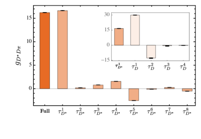
Figure 4: The contributions of different basis elements (see, eq. (19)) to the computed coupling constants. Further details and the exact values displayed are provided in table 2.

To further analyze this dissection, let us define $\{N_{H^{*}},N_{H}\}$ as the number of Dirac structures in the vector and pseudo-scalar meson BSAs, respectively, considered when evaluating $g_{H^{*}H\pi}$. Specifically, $N_{H^{*},H}=1$ would correspond to retaining only the leading BSA whereas $N_{H^{*},H}=8,4$ indicates the consideration of the complete basis. Our numerical results indicate that, when restricting the vector meson BSA to its dominant component, the resulting error in $g_{D^{*}D\pi}$ is approximately $2.5\%$, while for $g_{B^{*}B\pi}$, it increases up to $8.7\%$. Both are rather close to the complete results for $\{N_{H^{*}}=8,N_{H}={4}\}$, as the contributions from the other terms tend to cancel out each other. This suggests that $\{N_{H^{*}}=1,N_{H}=4\}$ provides a fairly good approximation, and the sub-dominant amplitudes of vector meson make only a minor correction, which is consistent with previous explorations concerning the $\rho\pi\pi$ process Tandy:1998ha .

This being the case, one can focus on retaining only the dominant BSA in the vector meson and thus analyze the contributions of the different pseudo-scalar meson BSAs. In contrast to the $H^{*}$ case, the contributions of the first two basis-elements of the $H$ meson BSA are both significant; and, in fact, the $\tau_{0^{-}}^{2}$ component (see eq. (19)) provides a non-negligible negative correction. Hence, the result for $\{N_{H^{*}}=1,N_{H}=1\}$ is approximately twice the complete result. This is not surprising, as the subdominant amplitude $\tau_{0^{-}}^{2}$ often plays an important role in accurately characterizing the properties of the pseudo-scalar (for instance, in determining the asymptotic behavior of its electromagnetic form factors), Maris:1998hc . Although employing a different effective interaction kernel, a similar conclusion for $D^{*}D\pi$ was reported in ref. daSilveira:2022pte , hence supporting our interpretation.

	$g_{D^{*}D\pi}$	$\hat{g}_{D}$	$g_{B^{*}B\pi}$	$\hat{g}_{B}$
This work	$16.22_{-0.01}^{+0.03}$	$0.55_{-<0.01}^{+<0.01}$	$40.09_{-1.37}^{+1.51}$	$0.50_{-0.02}^{+0.02}$
Experiment ParticleDataGroup:2022pth	$16.82\pm 0.25$	-	-	-
Lattice(16) Flynn:2015xna	-	-	${}^{*}45.3\pm 6.0$	$0.56\pm 0.07$
Lattice(15) Bernardoni:2014kla	-	-	-	$0.492\pm 0.029$
Lattice(13) Can:2012tx	$16.23\pm 1.71$	-	-	-
Lattice(13) Becirevic:2012pf	$15.8\pm 0.7$	$0.53\pm 0.03$	-	-
Lattice(12) Detmold:2012ge ; Detmold:2011bp	-	-	-	$0.449\pm 0.051$
DSE(23) daSilveira:2022pte	$17.24_{-2.30}^{+3.06}$	$0.58_{-0.08}^{+0.10}$	-	-
DSE(11) El-Bennich:2010uqs	$15.8_{-10}^{+2.1}$	$0.53_{-0.03}^{+0.07}$	$30.0_{-1.4}^{+3.2}$	$0.37_{-0.02}^{+0.04}$
SR(21) Khodjamirian:2020mlb	$14.1_{-1.2}^{+1.3}$	-	$30.0_{-2.4}^{+2.6}$	$0.30_{-0.02}^{+0.02}$
SR(06) Duraes:2004uc	$17.5\pm 1.5$	-	$44.7\pm 1.0$	-
SR(01) Navarra:2001ju	$14.0\pm 1.5$	-	$42.5\pm 2.6$	-
HQET(14) Cheung:2014cka	$16.8\mp 0.2$	$0.566_{+0.008}^{-0.007}$	$43.9_{-0.2}^{+0.1}$	$0.540_{-0.002}^{+0.001}$

Table 3: Comparison of our produced coupling constant with experimental values and other estimations. The script ^∗ denotes a calculation based on the formula provided in that paper. The experimental value of $g_{D^{*}D\pi}$ is derived from the $D^{+}\rightarrow D^{0}\pi^{+}$ data provided by PDG ParticleDataGroup:2022pth ; Khodjamirian:2020mlb .

In table 3, we compare our complete results of $g_{H^{*}H\pi}$ alongside predictions from other theoretical frameworks. Additionally, the value of $g_{D^{*}D\pi}$ extracted from experimental data is also listed. The PDG reports the total width of $D^{*\pm}$ to be:

$$\Gamma_{\text{tot }}\left(D^{*\pm}\right)=83.4\pm 1.8\ \text{keV}\,,$$ (27)

based on BaBar ($83.3\pm 1.2\pm 1.4$ keV) and CLEO ($96\pm 4\pm 22$ keV) determinations. According to the precisely measured branching fraction, $\mathcal{B}\mathcal{R}(D^{*+}\rightarrow D^{0}{\pi^{+}})=67.7\pm 0.5\%$, one has

$$\Gamma_{\text{PDG}}\left(D^{*+}\rightarrow D^{0}\pi^{+}\right) =56.5\pm 1.3\ \text{keV},$$ (28)

with BaBar ($56.4\pm 1.0$) keV and CLEO ($65\pm 15)$ keV. Correspondingly, $g_{D^{*}D\pi}$ can be extracted via the formula Belyaev:1994zk ; Khodjamirian:2020mlb :

$$\Gamma\left(D^{*+}\rightarrow D^{0}\pi^{+}\right) =\frac{g_{D^{*}D\pi}^{2}}{24\pi M_{D^{*}}^{2}}k^{3},$$ (29)

where

$$k^{2} =(M_{D^{*+}}^{2}-(M_{D^{+}}+M_{\pi^{+}})^{2})(M_{D^{*+}}^{2}-(M_{D^{+}}-M_{\pi^{+}})^{2})/4M_{D^{*+}}^{2}$$ (30)

$$=(39.33\pm 0.24)^{2}\ \text{MeV}^{2}\,,$$ (31)

hence arriving at

$$g^{\text{PDG}}_{D^{*}D\pi}=16.82\pm 0.25\,,$$ (32)

whereas one has BaBar $(16.81\pm 0.2)$ and CLEO $(18.0\pm 2.1)$.

The $B^{*}B\pi$ coupling cannot be measured directly, as the decay $B^{*}\rightarrow B\pi$ is kinematically forbidden. Nevertheless, $g_{B^{*}B\pi}$ remains of interest because it is closer to the heavy quark limit than $g_{D^{*}D\pi}$. As mentioned in the introduction, this makes it more suitable for accurately extracting the static strong coupling $\hat{g}$. Following Refs. Mader:2011zf ; daSilveira:2022pte ; Cheung:2014cka , we define

$$\hat{g}_{H}=\frac{g_{H^{*}H\pi}}{2\sqrt{M_{H}M_{H^{*}}}}f_{\pi}\,,$$ (33)

and obtain

$$\hat{g}_{D}=0.55_{-<0.01}^{+<0.01},\quad\hat{g}_{B}=0.50_{-0.02}^{+0.02}\,.$$ (34)

Our estimates are captured in table 3, which provides comparisons with other available results. Notably, the values $g_{D*D\pi}$ and $\hat{g}_{D}$ couplings obtained from different approaches, can deviate up to $20\%$ with respect to the experimental values, while our prediction lies within a $3.5\%$ range. The result reported in daSilveira:2022pte , denoted as DSE(23), is comparable to ours; therein, a DSEs/BSEs scheme was employed as well, albeit with a different effective heavy-light kernel. This agreement is encouraging as the cross-comparison of different effective heavy-light BSE kernels demonstrates the stability of the current computational framework. In addition, compared with DSE(23), we directly solved the corresponding BSEs in the moving frame, thereby eliminating the uncertainties associated with extrapolation or fitting procedures, which in turn reduces the error.

In the case of $g_{B*B\pi}$ and $\hat{g}_{B}$, the reported values from different models exhibit a larger discrepancy. This could be due to the higher flavor asymmetry, which presents theoretical challenges, as observed in the case of electromagnetic form factors Xu:2024fun . Our result is slightly lower than the central value of $\hat{g}_{B}=0.56\pm 0.07$ from the latest lattice result Flynn:2015xna , although it is still within the error bar. However, due to the absence of experimental data, these predictions still need to be further verified by different approaches.

4 Summary

In this work, we calculate the strong decay couplings $D^{*}D\pi$ and $B^{*}B\pi$ within a DSEs/BSEs based approach. This relies on the impulse approximation, along with a moving frame determination of the involved amplitudes. Notably, the $B^{*}B\pi$ result is reported for the first time based on a Poincaré invariant determination of the corresponding meson BSAs.

For the $D^{*}D\pi$ coupling, we predict $g_{D^{*}D\pi}=16.22_{-0.01}^{+0.03}$ and an associated static strong coupling $\hat{g}_{D}=0.55_{-<0.01}^{+<0.01}$, which differs from the coupling constant extracted from the PDG experimental data by about 3.5%. Since the BSEs are solved directly in the moving frame, errors due to fitting/extrapolation can be eliminated. The error reported in this work arises from the adjustment of the momentum partitioning parameter $\alpha$, which can be improved with a more accurate numerical integration. Moreover, our results are consistent with those obtained using a similar framework but with a different effective heavy-light BSE kernel. This cross-check demonstrates the stability of the current computational framework.

Concerning the $B^{*}B\pi$ case, we predict $g_{B^{*}B\pi}=40.09_{-1.37}^{+1.51}$ and $\hat{g}_{B}=0.50_{-0.02}^{+0.02}$, which are in good agreement with the most recent lattice results. However, in the absence of experimental data for validation, these predictions should be further corroborated through the application of alternative models or approaches.

Finally, we recall that our calculation exploits the impulse approximation, which allows expressing the quantities of interest in terms of quark propagators meson BSAs. These are obtained under a RL-like framework that employs an effective heavy-light kernel. Therefore, further comparisons based on other possible effective kernels are crucial. Moreover, the results should be refined in the future by developing a more advance approach that goes beyond the RL kernel/impulse approximation. In any case, the scheme herein presented can be straightforwardly applied to investigate other strong decay processes. More broadly, we anticipate that it will be valuable for investigating the static properties and dynamics of QCD’s bound-states.

Appendix A Decoupling of BSEs and lossless kernel matrix compression

As mentioned in section 3, compared to the rest frame, the memory requirements for solving the BSEs in a moving frame typically increase by two orders of magnitude ($\sim$ TB), making related optimizations crucial. We thus rewrite eq. (17) as

$$\Gamma(k;P)=\int^{\Lambda}\frac{d^{4}q}{(2\pi)^{4}}\tilde{\mathcal{D}}^{\mu\nu}_{\text{eff}}(k-q)\gamma_{\mu}S\left(q_{+}\right)\Gamma(q;P)S\left(q_{-}\right)\gamma_{\nu},$$ (35)

where the RL approximation has been applied, and

$$\Gamma(k;P)=F_{i}(k,P)\tau_{i}(k,P)\,.$$ (36)

For convenience, we use the Einstein summation convention in the appendix. Here $\tau_{i}(k,P)$ defines the basis elements (see, eq. (19)) and $F_{i}(k,P)$ is the associated scalar functions. Therefore eq. (35) can be expanded as

$$F_{i}(k,P)\tau_{i}(k,P)=\int^{\Lambda}\frac{d^{4}q}{(2\pi)^{4}}\tilde{\mathcal{D}}^{\mu\nu}_{\text{eff}}(k-q)\gamma_{\mu}S\left(q_{+}\right)F_{\alpha}(q,P)\tau_{\alpha}(q,P)S\left(q_{-}\right)\gamma_{\nu}\,.$$ (37)

Multiplying both sides of eq. (37) by each of the basis elements, and taking the trace over the Dirac indices, yields the following:

$$\text{Tr}(\tau_{j}(k,P)\tau_{i}(k,P))F_{i}(k,P)$$

$$= \int^{\Lambda}\frac{d^{4}q}{(2\pi)^{4}}\tilde{\mathcal{D}}^{\mu\nu}_{\text{eff}}(k-q)\text{Tr}(\tau_{j}(k,P)\gamma_{\mu}S\left(q_{+}\right)\tau_{\alpha}(q,P)S\left(q_{-}\right)\gamma_{\nu})F_{\alpha}(q,P)\,.$$ (38)

To express it more concisely, we have:

$$\mathscr{P}^{(1)}_{ji}({k,P})F_{i}(k,P)=\int^{\Lambda}\frac{d^{4}q}{(2\pi)^{4}}\mathscr{M}_{j\alpha}({k,q,P})F_{\alpha}(q,P),$$ (39)

where we define two matrices which don’t have Dirac structure:

$$\mathscr{P}^{(1)}_{ji}({k,P}) \equiv\text{Tr}(\tau_{j}(k,P)\tau_{i}(k,P)),$$ (40)

$$\mathscr{M}^{(0)}_{j\alpha}({k,q,P}) \equiv\text{Tr}(\tilde{\mathcal{D}}^{\mu\nu}_{\text{eff}}(k-q)\tau_{j}(k,P)\gamma_{\mu}S\left(q_{+}\right)\tau_{\alpha}(q,P)S\left(q_{-}\right)\gamma_{\nu}).$$ (41)

Finally, eq. (35) is decoupled into

$$F_{i}(k,P)=\int^{\Lambda}\frac{d^{4}q}{(2\pi)^{4}}\mathscr{M}^{(1)}_{ij}({k,P})\mathscr{M}^{(0)}_{j\alpha}({k,q,P})F_{\alpha}(q,P)\,,$$ (42)

where $\mathscr{M}^{(1)}(k,P)$ is the inverse matrix of $\mathscr{P}^{(1)}(k,P)$. After discretization using numerical integration, eq. (42) turns into an eigenvalue equation, and the scalar function $F(k,P)$ can be directly obtained. However, the matrix $\mathscr{M}^{(0)}(k,q,P)$ typically does not have non-zero matrix elements. Therefore, it requires a substantial amount of memory resources, particularly in the numerical computations of moving frame BSEs.

Note that when the basis is complete, the BS wave function $\chi(q,P)\equiv S\left(q_{+}\right)\Gamma(q;P)S\left(q_{-}\right)$ can be expanded in the same basis

$$\chi(q,P)=g_{\alpha}(q,P)\tau_{\alpha}(q,P)\,,$$ (43)

with corresponding $g_{\alpha}(q,P)$ scalar functions. These can be written as

$$g_{\sigma}(q,P) =\delta_{\sigma\alpha}g_{\alpha}(q,P)$$ (44)

$$=\mathscr{M}^{(1)}_{\sigma\beta}(q,P)\mathscr{P}^{(1)}_{\beta\alpha}(q,P)g_{\alpha}(q,P)$$ (45)

$$=\mathscr{M}^{(1)}_{\sigma\beta}(q,P)\text{Tr}(\tau_{\beta}(q,P)g_{\alpha}(q,P)\tau_{\alpha}(q,P))$$ (46)

$$=\mathscr{M}^{(1)}_{\sigma\beta}(q,P)\text{Tr}(\tau_{\beta}(q,P)\chi(q,P))\,,$$ (47)

such that

$$\chi(q,P) =g_{\sigma}(q,P)\tau_{\sigma}(q,P)$$ (48)

$$=\mathscr{M}^{(1)}_{\sigma\beta}(q,P)\text{Tr}(\tau_{\beta}(q,P)\chi(q,P))\tau_{\sigma}(q,P)$$ (49)

$$=\mathscr{M}^{(1)}_{\sigma\beta}(q,P)\text{Tr}(\tau_{\beta}(q,P)S\left(q_{+}\right)\Gamma(q;P)S\left(q_{-}\right))\tau_{\sigma}(q,P)$$ (50)

$$=\mathscr{M}^{(1)}_{\sigma\beta}(q,P)\text{Tr}(\tau_{\beta}(q,P)S\left(q_{+}\right)F_{\alpha}(q,P)\tau_{\alpha}(q,P)S\left(q_{-}\right))\tau_{\sigma}(q,P)$$ (51)

$$=\mathscr{M}^{(1)}_{\sigma\beta}(q,P)\text{Tr}(\tau_{\beta}(q,P)S\left(q_{+}\right)\tau_{\alpha}(q,P)S\left(q_{-}\right))F_{\alpha}(q,P)\tau_{\sigma}(q,P)$$ (52)

$$=\mathscr{M}^{(1)}_{\sigma\beta}(q,P)\mathscr{M}^{(2)}_{\beta\alpha}(q,P)F_{\alpha}(q,P)\tau_{\sigma}(q,P),$$ (53)

where we have defined

$$\mathscr{M}^{(2)}_{\beta\alpha}(q,P)\equiv\text{Tr}(\tau_{\beta}(q,P)S\left(q_{+}\right)\tau_{\alpha}(k,P)S\left(q_{-}\right))\,.$$ (54)

Therefore, eq. (35) can be cast as

$$\Gamma(k;P) =\int^{\Lambda}\frac{d^{4}q}{(2\pi)^{4}}\tilde{\mathcal{D}}^{\mu\nu}_{\text{eff}}\gamma_{\mu}\chi(q,P)\gamma_{\nu}$$ (55)

$$=\int^{\Lambda}\frac{d^{4}q}{(2\pi)^{4}}\tilde{\mathcal{D}}^{\mu\nu}_{\text{eff}}\gamma_{\mu}\mathscr{M}^{(1)}_{\sigma\beta}(q,P)\mathscr{M}^{(2)}_{\beta\alpha}(q,P)F_{\alpha}(q,P)\tau_{\sigma}(q,P)\gamma_{\nu}.$$ (56)

Similar to eqs. (37)-(42), the BSAs are expanded and then decoupled, thus producing

$$\text{Tr}(\tau_{j}(k,P)F_{i}(k,P)\tau_{i}(k,P))$$

$$= \int^{\Lambda}\frac{d^{4}q}{(2\pi)^{4}}\tilde{\mathcal{D}}^{\mu\nu}_{\text{eff}}\text{Tr}(\tau_{j}(k,P)\gamma_{\mu}\tau_{\sigma}(q,P)\gamma_{\nu})\mathscr{M}^{(1)}_{\sigma\beta}(q,P)\mathscr{M}^{(2)}_{\beta\alpha}(q,P)F_{\alpha}(q,P)\,.$$ (57)

Subsequently, eq. (57) can be written more concisely as

$$\mathscr{P}_{ji}(k,P)F_{i}(k,P)=\int^{\Lambda}\frac{d^{4}q}{(2\pi)^{4}}\mathscr{M}_{j\sigma}^{(3)}(k,q,P)\mathscr{M}^{(1)}_{\sigma\beta}(q,P)\mathscr{M}^{(2)}_{\beta\alpha}(q,P)F_{\alpha}(q,P)\,,$$ (58)

where

$$\mathscr{M}_{j\sigma}^{(3)}(k,q,P)\equiv\text{Tr}(\tilde{\mathcal{D}}^{\mu\nu}_{\text{eff}}\tau_{j}(k,P)\gamma_{\mu}\tau_{\sigma}(q,P)\gamma_{\nu})\,.$$ (59)

Finally, eq. (35) is decoupled into

$$F_{i}(k,P)=\int^{\Lambda}\frac{d^{4}q}{(2\pi)^{4}}\mathscr{M}^{(1)}_{ij}(k,P)\mathscr{M}_{j\sigma}^{(3)}(k,q,P)\mathscr{M}^{(1)}_{\sigma\beta}(q,P)\mathscr{M}^{(2)}_{\beta\alpha}(q,P)F_{\alpha}(q,P).$$ (60)

Compared to eq. (42), the decoupling method used in eq. (60) results in a substantial number of zero-valued matrix elements in the $\mathscr{M}^{(3)}(k,q,P)$, which allows for the storage of only the non-zero elements, thereby saving memory. In this work, memory usage for $4\times 4$ pseudo-scalar case can be cut down to $6/16\sim 38\%$, while for $8\times 8$ vector case, it is reduced to $20/64\sim 31\%$.

- (1) HFLAV collaboration, Averages of b-hadron, c-hadron, and -lepton properties as of 2021, Phys. Rev. D 107 (2023) 052008 [2206.07501].
- (2) RBC, UKQCD collaboration, The Coupling Using Relativistic Heavy Quarks, Phys. Rev. D 93 (2016) 014510 [1506.06413].
- (3) V.M. Belyaev, V.M. Braun, A. Khodjamirian and R. Ruckl, D* D pi and B* B pi couplings in QCD, Phys. Rev. D 51 (1995) 6177 [hep-ph/9410280].
- (4) A. Khodjamirian, B. Melić, Y.-M. Wang and Y.-B. Wei, The and couplings from light-cone sum rules, JHEP 03 (2021) 016 [2011.11275].
- (5) G. Burdman and J.F. Donoghue, Union of chiral and heavy quark symmetries, Phys. Lett. B 280 (1992) 287.
- (6) M.B. Wise, Chiral perturbation theory for hadrons containing a heavy quark, Phys. Rev. D 45 (1992) R2188.
- (7) T.-M. Yan, H.-Y. Cheng, C.-Y. Cheung, G.-L. Lin, Y.C. Lin and H.-L. Yu, Heavy quark symmetry and chiral dynamics, Phys. Rev. D 46 (1992) 1148.
- (8) ALPHA collaboration, Precision lattice QCD computation of the coupling, Phys. Lett. B 740 (2015) 278 [1404.6951].
- (9) K.U. Can, G. Erkol, M. Oka, A. Ozpineci and T.T. Takahashi, Vector and axial-vector couplings of D and D* mesons in 2+1 flavor Lattice QCD, Phys. Lett. B 719 (2013) 103 [1210.0869].
- (10) D. Becirevic and F. Sanfilippo, Theoretical estimate of the decay rate, Phys. Lett. B 721 (2013) 94 [1210.5410].
- (11) W. Detmold, C.J.D. Lin and S. Meinel, Calculation of the heavy-hadron axial couplings , and using lattice QCD, Phys. Rev. D 85 (2012) 114508 [1203.3378].
- (12) W. Detmold, C.J.D. Lin and S. Meinel, Axial couplings and strong decay widths of heavy hadrons, Phys. Rev. Lett. 108 (2012) 172003 [1109.2480].
- (13) C.-Y. Cheung and C.-W. Hwang, Strong and radiative decays of heavy mesons in a covariant model, JHEP 04 (2014) 177 [1401.3917].
- (14) F.O. Duraes, F.S. Navarra, M. Nielsen and M.R. Robilotta, Meson loops and the g(D*D pi) coupling, Braz. J. Phys. 36 (2006) 1232 [hep-ph/0403064].
- (15) F.S. Navarra, M. Nielsen and M.E. Bracco, D* D pi form-factor revisited, Phys. Rev. D 65 (2002) 037502 [hep-ph/0109188].
- (16) D. Jarecke, P. Maris and P.C. Tandy, Strong decays of light vector mesons, Phys. Rev. C 67 (2003) 035202 [nucl-th/0208019].
- (17) V. Mader, G. Eichmann, M. Blank and A. Krassnigg, Hadronic decays of mesons and baryons in the Dyson-Schwinger approach, Phys. Rev. D 84 (2011) 034012 [1106.3159].
- (18) B. El-Bennich, M.A. Ivanov and C.D. Roberts, Strong D* - D+pi and B* - B+pi couplings, Phys. Rev. C 83 (2011) 025205 [1012.5034].
- (19) R.C. da Silveira, F.E. Serna and B. El-Bennich, Strong two-meson decays of light and charmed vector mesons, Phys. Rev. D 107 (2023) 034021 [2211.16618].
- (20) C.D. Roberts and A.G. Williams, Dyson-Schwinger equations and their application to hadronic physics, Prog. Part. Nucl. Phys. 33 (1994) 477 [hep-ph/9403224].
- (21) P. Maris, C.D. Roberts and P.C. Tandy, Pion mass and decay constant, Phys. Lett. B 420 (1998) 267 [nucl-th/9707003].
- (22) P. Maris and C.D. Roberts, Pi- and K meson Bethe-Salpeter amplitudes, Phys. Rev. C 56 (1997) 3369 [nucl-th/9708029].
- (23) P. Maris and P.C. Tandy, Bethe-Salpeter study of vector meson masses and decay constants, Phys. Rev. C 60 (1999) 055214 [nucl-th/9905056].
- (24) S.-x. Qin, L. Chang, Y.-x. Liu, C.D. Roberts and D.J. Wilson, Interaction model for the gap equation, Phys. Rev. C 84 (2011) 042202 [1108.0603].
- (25) S.-x. Qin, L. Chang, Y.-x. Liu, C.D. Roberts and D.J. Wilson, Investigation of rainbow-ladder truncation for excited and exotic mesons, Phys. Rev. C 85 (2012) 035202 [1109.3459].
- (26) K. Raya, L. Chang, A. Bashir, J.J. Cobos-Martinez, L.X. Gutiérrez-Guerrero, C.D. Roberts et al., Structure of the neutral pion and its electromagnetic transition form factor, Phys. Rev. D 93 (2016) 074017 [1510.02799].
- (27) G. Eichmann, H. Sanchis-Alepuz, R. Williams, R. Alkofer and C.S. Fischer, Baryons as relativistic three-quark bound states, Prog. Part. Nucl. Phys. 91 (2016) 1 [1606.09602].
- (28) C.S. Fischer, QCD at finite temperature and chemical potential from Dyson–Schwinger equations, Prog. Part. Nucl. Phys. 105 (2019) 1 [1810.12938].
- (29) P. Qin, S.-x. Qin and Y.-x. Liu, Heavy-light mesons beyond the ladder approximation, Phys. Rev. D 101 (2020) 114014 [1912.05902].
- (30) M. Chen and L. Chang, A pattern for the flavor dependent quark-antiquark interaction, Chin. Phys. C 43 (2019) 114103 [1903.07808].
- (31) Y.-Z. Xu, D. Binosi, Z.-F. Cui, B.-L. Li, C.D. Roberts, S.-S. Xu et al., Elastic electromagnetic form factors of vector mesons, Phys. Rev. D 100 (2019) 114038 [1911.05199].
- (32) F.E. Serna, R.C. da Silveira, J.J. Cobos-Martínez, B. El-Bennich and E. Rojas, Distribution amplitudes of heavy mesons and quarkonia on the light front, Eur. Phys. J. C 80 (2020) 955 [2008.09619].
- (33) Y.-Z. Xu, C. Shi, X.-T. He and H.-S. Zong, Chiral crossover transition from the Dyson-Schwinger equations in a sphere, Phys. Rev. D 102 (2020) 114011 [2009.12035].
- (34) Y.-Z. Xu, S.-X. Qin and H.-S. Zong, Chiral symmetry restoration and properties of Goldstone bosons at finite temperature*, Chin. Phys. C 47 (2023) 033107 [2106.13592].
- (35) Y.-Z. Xu, S. Chen, Z.-Q. Yao, D. Binosi, Z.-F. Cui and C.D. Roberts, Vector-meson production and vector meson dominance, Eur. Phys. J. C 81 (2021) 895 [2107.03488].
- (36) F.E. Serna, R.C. da Silveira and B. El-Bennich, D* and Ds* distribution amplitudes from Bethe-Salpeter wave functions, Phys. Rev. D 106 (2022) L091504 [2209.09278].
- (37) Q. Li, C.-H. Chang, T. Wang and G.-L. Wang, Strong decays of to J/(c)p and within the Bethe-Salpeter framework, JHEP 06 (2023) 189 [2301.02094].
- (38) Y.-Z. Xu and J. Segovia, An Assessment of Pseudoscalar and Vector Meson Electromagnetic Form Factors, Few Body Syst. 64 (2023) 62.
- (39) Y.-Z. Xu, M. Ding, K. Raya, C.D. Roberts, J. Rodríguez-Quintero and S.M. Schmidt, Pion and kaon electromagnetic and gravitational form factors, Eur. Phys. J. C 84 (2024) 191 [2311.14832].
- (40) Y.Z. Xu, K. Raya, J. Rodríguez-Quintero and J. Segovia, Charge distributions of pseudoscalar and vector mesons from Dyson-Schwinger equations, Phys. Rev. D 110 (2024) 054031 [2406.13306].
- (41) K. Raya, A. Bashir, D. Binosi, C.D. Roberts and J. Rodríguez-Quintero, Pseudoscalar Mesons and Emergent Mass, Few Body Syst. 65 (2024) 60 [2403.00629].
- (42) Y.-Z. Xu, The electromagnetic form factors of heavy-light pseudo-scalar and vector mesons, JHEP 07 (2024) 118 [2402.06141].
- (43) C. Shi, P. Liu, Y.-L. Du and W. Jia, Heavy flavor-asymmetric pseudoscalar mesons on the light front, Phys. Rev. D 110 (2024) 094010 [2409.05098].
- (44) Particle Data Group collaboration, Review of Particle Physics, PTEP 2022 (2022) 083C01.
- (45) M.S. Bhagwat and P. Maris, Vector meson form factors and their quark-mass dependence, Phys. Rev. C 77 (2008) 025203 [nucl-th/0612069].
- (46) L. Chang, Y.-x. Liu, C.D. Roberts, Y.-m. Shi, W.-m. Sun and H.-s. Zong, Chiral susceptibility and the scalar Ward identity, Phys. Rev. C 79 (2009) 035209 [0812.2956].
- (47) P. Maris and C.D. Roberts, Dyson-Schwinger equations: A Tool for hadron physics, Int. J. Mod. Phys. E 12 (2003) 297 [nucl-th/0301049].
- (48) C.S. Fischer, P. Watson and W. Cassing, Probing unquenching effects in the gluon polarisation in light mesons, Phys. Rev. D 72 (2005) 094025 [hep-ph/0509213].
- (49) E. Rojas, B. El-Bennich and J.P.B.C. de Melo, Exciting flavored bound states, Phys. Rev. D 90 (2014) 074025 [1407.3598].
- (50) H. Sanchis-Alepuz and R. Williams, Recent developments in bound-state calculations using the Dyson–Schwinger and Bethe–Salpeter equations, Comput. Phys. Commun. 232 (2018) 1 [1710.04903].
- (51) A. Windisch, Analytic properties of the quark propagator from an effective infrared interaction model, Phys. Rev. C 95 (2017) 045204 [1612.06002].
- (52) M.A. Sultan, K. Raya, F. Akram, A. Bashir and B. Masud, Effect of the quark-gluon vertex on dynamical chiral symmetry breaking, Phys. Rev. D 103 (2021) 054036 [1810.01396].
- (53) F.E. Serna, B. El-Bennich and G.a. Krein, Charmed mesons with a symmetry-preserving contact interaction, Phys. Rev. D 96 (2017) 014013 [1703.09181].
- (54) H.J. Munczek, Dynamical chiral symmetry breaking, Goldstone’s theorem and the consistency of the Schwinger-Dyson and Bethe-Salpeter Equations, Phys. Rev. D 52 (1995) 4736 [hep-th/9411239].
- (55) R.J. Dowdall, C.T.H. Davies, T.C. Hammant and R.R. Horgan, Precise heavy-light meson masses and hyperfine splittings from lattice QCD including charm quarks in the sea, Phys. Rev. D 86 (2012) 094510 [1207.5149].
- (56) K. Cichy, M. Kalinowski and M. Wagner, Continuum limit of the meson, meson and charmonium spectrum from twisted mass lattice QCD, Phys. Rev. D 94 (2016) 094503 [1603.06467].
- (57) ETM collaboration, Masses and decay constants of D*(s) and B*(s) mesons with N twisted mass fermions, Phys. Rev. D 96 (2017) 034524 [1707.04529].
- (58) A. Bazavov et al., - and -meson leptonic decay constants from four-flavor lattice QCD, Phys. Rev. D 98 (2018) 074512 [1712.09262].
- (59) M. Ding, F. Gao, L. Chang, Y.-X. Liu and C.D. Roberts, Leading-twist parton distribution amplitudes of S-wave heavy-quarkonia, Phys. Lett. B 753 (2016) 330 [1511.04943].
- (60) M.A. Ivanov, Y.L. Kalinovsky and C.D. Roberts, Survey of heavy meson observables, Phys. Rev. D 60 (1999) 034018 [nucl-th/9812063].
- (61) M. Gómez-Rocha, T. Hilger and A. Krassnigg, Effects of a dressed quark-gluon vertex in vector heavy-light mesons and theory average of the meson mass, Phys. Rev. D 93 (2016) 074010 [1602.05002].
- (62) S.-X. Qin and C.D. Roberts, Resolving the Bethe–Salpeter Kernel, Chin. Phys. Lett. 38 (2021) 071201 [2009.13637].
- (63) P.C. Tandy, Electromagnetic form-factors of meson transitions, Fizika B 8 (1999) 295 [hep-ph/9902459].
- (64) P. Maris and C.D. Roberts, Pseudovector components of the pion, pi0 — gamma gamma, and F(pi) (q**2), Phys. Rev. C 58 (1998) 3659 [nucl-th/9804062].