Enhancing Blind Source Separation with Dissociative Principal Component Analysis

Abstract

Sparse principal component analysis (sPCA) enhances the interpretability of principal components (PCs) by imposing sparsity constraints on loading vectors (LVs). However, when used as a precursor to independent component analysis (ICA) for blind source separation (BSS), sPCA may underperform due to its focus on simplicity, potentially disregarding some statistical information essential for effective ICA. To overcome this limitation, a sophisticated approach is proposed that preserves the interpretability advantages of sPCA while significantly enhancing its source extraction capabilities. This consists of two tailored algorithms, dissociative PCA (DPCA1 and DPCA2), which employ adaptive and firm thresholding alongside gradient and coordinate descent approaches to optimize the proposed model dynamically. These algorithms integrate left and right singular vectors from singular value decomposition (SVD) through dissociation matrices (DMs) that replace traditional singular values, thus capturing latent interdependencies effectively to model complex source relationships. This leads to refined PCs and LVs that more accurately represent the underlying data structure. The proposed approach avoids focusing on individual eigenvectors, instead, it collaboratively combines multiple eigenvectors to disentangle interdependencies within each SVD variate. The superior performance of the proposed DPCA algorithms is demonstrated across four varied imaging applications including functional magnetic resonance imaging (fMRI) source retrieval, foreground-background separation, image reconstruction, and image inpainting. They outperformed traditional methods such as PCA+ICA, PPCA+ICA, SPCA+ICA, PMD, and GPower.

Introduction

Principal component analysis first introduced in the early twentieth century [1], has been widely employed for data processing, feature extraction, and dimension reduction across various fields, including signal and image processing, machine learning, and exploratory data analysis [2]. It projects high-dimensional, correlated data into a lower-dimensional subspace, which is defined by uncorrelated PCs and spanned by orthogonal LVs [3, 4]. These PCs preserve the majority of the statistical information in the data [5]. This makes PCA a powerful multivariate statistical technique that can be utilized to reveal true dimensionality of the data [6] and usually deployed as a preprocessing step for BSS algorithms [7].

Principal components, however, are difficult to interpret [8] because each of them is a linear combination of all variables from original feature space. To address this shortcoming, several sparse variants of PCA have been proposed [9] that seek to balance interpretability and statistical fidelity by constructing PCs from a minimal number of variables, while retaining as much of the statistical information in the data as possible. On the other hand, sPCA is computationally intractable because it imposes a cardinality constraint on the LVs [10]. To tackle this issue, numerous approximate algorithms have been developed to achieve a solution that is nearly optimal, by striking a balance between computational efficiency and sparsity [11].

Sparse PCA is an optimization problem whose objectives are to maximize the variance explained by the PCs while simultaneously achieving sparsity for the LVs [12]. For instance, a first effort at sparse PCA resulted in simplified component technique with LASSO (SCoTLASS) [13], which aimed at maximizing the Rayleigh quotient under $l_{1}$ norm penalty, a regression-based optimization problem with LASSO penalty led to sparse PCA (SPCA) [14], a convex relaxation of the sparse PCA problem using semidefinite programming (SDP) produced DSPCA method [15], a framework that considered the covariance matrix for SVD with $l_{1}$ penalties on left and right singular vectors culminated in penalized matrix decomposition (PMD) [16], lastly, a novel iterative thresholding approach was introduced, effectively estimating principal subspaces and leading eigenvectors, marking further progress in sparse PCA methodologies [17].

Computationally effective techniques for sparse PCA were subsequently developed. Notably, the generalized power method (GPower), which involved maximizing a convex function on a compact set [18]. Later, an effective solution to non-convex sparse eigenvalue problems known as the truncated power method (TPower) was introduced [19]. Innovative methods for sparse PCA have emerged in recent years. For instance, a Bayesian approach that generated components with common sparsity patterns [20], an adaptive block sparse PCA method called preserved PCA (PPCA) maintained sparsity across all LVs through group LASSO with adaptive penalization [6], an efficient online sparse PCA algorithm that combined gradient-based optimization techniques with stochastic gradient descent [21], and a recent method that improved sparsity by applying orthogonal rotation to PCs before thresholding [22].

While sPCA enhances the interpretability of PCs by enforcing sparsity, which is characterized by fewer non-zero entries, it often fails to strike an effective balance between interpretability and source separation. Traditional sPCA uses a deflation strategy that, while simplifying component interpretation, may mask the complex variable interrelationships, thus diminishing the significance of subsequent PCs, potentially distorting the data’s overall representation, which is vital for subsequent ICA as highlighted in [6]. In contrast, traditional PCA lacks interpretability and, when followed by ICA, may not effectively separate sources, particularly in scenarios with significant spatial overlaps [23, 24, 25]. Ultimately, both sPCA+ICA and PCA+ICA configurations may be suboptimal for achieving reliable source separation.

To date, no study has addressed the challenges inherent in sPCA and its integration with ICA for the separation of non-orthogonal independent components under conditions of moderate to significant spatial overlaps [25]. This study seeks to fill this research gap by extending the capabilities of sPCA. The main objective is to not only enhance the interpretability of PCs but also to significantly strengthen the robustness of source separation. The proposed DPCA is a novel methodology designed to minimize the interdependencies among PCA components. DPCA aims to deliver enhanced accuracy and reliability in source separation while maintaining and even improving the interpretability of each component, particularly in scenarios with substantial spatial overlaps.

This study has made several key contributions. Firstly, it uniquely models the interdependencies within both LVs and PCs, effectively capturing spatiotemporal ground truth. Secondly, two novel algorithms are introduced that integrate adaptive thresholding with gradient and coordinate descent, streamlining the solution process for the proposed optimization model in dissociative PCA. Thirdly, a secondary layer of firm thresholding is implemented to preserve sparsity and effectively remove background noise from modified LVs, thus enhancing their interpretability and separation simultaneously. Moreover, the model adapts seamlessly to function as ordinary PCA when the sparsity parameter is reduced to zero as shown in Proposition $2$ in the next section.

I Methods and Materials

I-A Background

Principal component analysis is most effective when a reduced number of components, $K<p$, is sufficient to capture the majority of the variance, thereby providing a simpler, yet insightful, representation of the underlying structure of the data. For this purpose, consider the data matrix $\text{X}\in\mathbb{R}^{n\times p}$ whose each column is mean-centered and with rank $K\leq\min(n,p)$, where X consists of $n$ observations on $p$ variables. In order to find a linear projection of the data that maximizes the variance retained in the lower-dimensional subspace, PCA seeks to solve the following constrained optimization problem that reduces the dimensionality of the data from $p$ to $K$ [26]

$$\arg\max_{\text{w}_{i}}\ \ \mathrm{var}(\text{X}\text{w}_{i})\quad\textrm{sub.to.}\ \ \text{w}_{i}^{\top}\text{w}_{i}=1,$$

$$\hskip 128.0374pt\text{w}_{i}^{\top}\text{w}_{j}=0\ \ \mathrm{for}\ \ i\neq j$$

where, $\text{w}_{i}$ represents the $i$-th principal LV, projection of the data $\text{X}\text{w}_{i}$ defines the $i$-th PC, and the operator $\mathrm{var}(.)$ refers to the variance of a given variable. The contribution of $\text{X}\text{w}_{i}$ explains $100\times\lambda_{i}/\sum_{j=1}^{p}\lambda_{j}$ percent of the total variance in the data, where $\lambda_{i}$ is the $i$-th eigenvalue. The solution of the above optimization problem is found in the following decomposition

$$\mathcal{C}=\sum_{i=1}^{k}\lambda_{i}\text{w}_{i}\text{w}_{i}^{\top}$$ (1)

where $\mathcal{C}=1/n(\text{X}^{\top}\text{X})$ represents covariance matrix, and $\lambda_{i}$ is the $i$-th largest eigenvalue, with $\text{w}_{i}$ as the corresponding eigenvector. Based on a linear regression approach, an alternative formulation of PCA can be obtained by solving the following least squares problem to estimate the projection matrix W that contains the $K$ LVs as [14]

$$\text{W}=\arg\min_{\text{W}}\ \ \sum_{j=1}^{n}\left\lVert{\text{x}^{j}}^{\top}-\text{W}\text{W}^{\top}{\text{x}^{j}}^{\top}\right\rVert_{2}^{2}$$

$$\hskip 22.76228pt\textrm{sub.to.}\ \ \text{W}^{\top}\text{W}=\text{I}_{K}$$ (2)

Usually, PCA is performed through the SVD of the data matrix X, which is expressed as

$$\text{X}=\text{UD}\text{W}^{\top}$$ (3)

In this decomposition, the columns in matrix UD contains the PCs, the matrix W holds the LVs as its columns, and the diagonal matrix $\text{D}\in\mathbb{R}^{K\times K}$ contains the singular values along the diagonal that is $\text{d}_{1}\geq\text{d}_{2}\geq\ldots\geq\text{d}_{K}>0$, ordered from largest to smallest. Both $\text{U}\in\mathbb{R}^{n\times K}$, which contains the left singular vectors and $\text{W}\in\mathbb{R}^{p\times K}$, which contains the right singular vectors are orthonormal matrices, satisfying $\text{U}^{\top}\text{U}=\text{W}^{\top}\text{W}=\text{I}_{K}$, where $\text{I}_{K}$ is the identity matrix of size $K\times K$. If equation (1) can be reformulated as $\mathcal{C}=\text{W}\Lambda\text{W}^{\top}$ then it is related to singular values in equation (3) as $\text{D}=|\Lambda|$. Because non-negative singular values in SVD provide a stable and interpretable transformation, in the subsequent section, equation (3) will be utilized as the basis for introducing the proposed model.

The proposed method distinctly differs from sparse dictionary learning approaches, such as those described in [27], which typically involve learning an overcomplete dictionary where $K>>n$ and a sparse code directly from the data. In contrast, the proposed approach limits the number of components to $K\leq n$. Rather than learning a dictionary and sparse codes anew, it utilizes predefined PCs and LVs to model the data, adapting existing structures to enhance computational efficiency and interpretability.

I-B Proposed Model

This study proceeds under the assumption that each column of the observed data matrix X is mean-centered, unless stated otherwise. Additionally, the number of PCs, $K$, is predetermined. For methodologies on determining $K$ from the data, reader is referred to this article [28], which discusses the use of cross-validated eigenvalues among other techniques. Particulary, for this paper, $K$ is selected based on performance metrics such as peak signal-to-noise ratio (PSNR) and the correlation strength between the ground truth and the reconstructed components.

This section presents the dissociative PCA method designed to effectively disentangle interdependencies within PCs and LVs. The proposed method uses a sequential estimating procedure for both PCs and LVs, in contrast to conventional sparse PCA methods that often use a deflation strategy that may overlook important interdependencies and compromise source separation effectiveness. By employing both coordinate descent and gradient descent techniques, the proposed approach not only enhances the accuracy of source separation but also improves the interpretability of the results.

Consider the matrix $\text{X}\in\mathbb{R}^{n\times p}$, represented in low-rank form as $\text{U}_{q}\text{D}_{q}\text{W}_{q}^{\top}$, where $K\leq\min(n,p)$. In this representation, $\text{U}_{q}\in\mathbb{R}^{n\times K}$ and $\text{W}_{q}\in\mathbb{R}^{p\times K}$ are orthogonal matrices, while $\text{D}_{q}\in\mathbb{R}^{K\times K}$ is a diagonal matrix of singular values. Left and right dissociative matrices $\Psi\in\mathbb{R}^{K\times K}$ and $\Phi\in\mathbb{R}^{K\times K}$ are introduced here to encapsulate interdependencies within the PCs and LVs, thereby modifying the traditional SVD framework, and its reformulation is expressed as

$$\text{X}=\text{U}_{q}\text{D}_{q}\text{W}_{q}^{\top}=\text{U}_{q}\Psi\Psi^{-1}\text{D}_{q}\Phi^{-1}\Phi\text{W}_{q}^{\top}=\text{U}\text{V}\text{W}^{\top}$$ (4)

This approach enhances the effectiveness of the model by applying sparsity constraints to W, ensuring that the decomposition $\text{U}\text{V}\text{W}^{\top}$ accurately represents the underlying data structure. The model leverages the $l_{1}$ norm to induce sparsity, effectively managing column sparsity. Further details on this implementation are provided in subsequent subsections.

After the estimation of $\Psi$ and $\Phi$, the non-diagonal middle matrix $\text{V}=\Psi^{-1}\text{D}_{q}\Phi^{-1}$ facilitates understanding of the interactions between PCs and LVs. It is a diagonal matrix for a standard PCA, however, when sparsity is enforced on W, the matrix V may exhibit small off-diagonal values, indicating interdependencies among the LVs. While DMs allow to break the interdependencies within PCs and within LVs, the weighing matrix V captures the extent of these interdependencies.

Because the estimation of U and W is not contingent upon V, I can adjust or even exclude V without altering the structural integrity of U and W. This flexibility allows for an alternative decomposition where V is omitted. Considering that both $\text{U}\text{W}^{\top}$ and $\text{U}\text{V}\text{W}^{\top}$ can serve as approximate estimates of both X and the traditional $\text{U}_{q}\text{D}_{q}\text{W}_{q}^{\top}$, hence the following simplified decomposition is proposed

$$\text{X}=\text{U}\text{W}^{\top}$$ (5)

This model retains the essential properties of the original decomposition while incorporating dissociation, which, according to proposition $1$, also preserves key aspects of the original variance structure.

Proposition 1: For a given rank $K$ matrix X, the solution $\text{U}\text{W}^{\top}$ achieved through the dissociation process using $\Psi$ and $\Phi$ enhances interpretability and facilitates effective source separation by adjusting the amount of variance each component explains.
Proof: The dissociation matrices $\Psi$ and $\Phi$ modify the singular values in $\text{D}_{q}$ to produce the new singular value matrix $\hat{\text{D}}_{q}=\Psi\Phi$. Unlike the original diagonal matrix $\text{D}_{q}$ with singular values in descending order $\text{d}_{q,1}\geq\text{d}_{q,2}\geq\ldots\geq\text{d}_{q,K}>0$, $\hat{\text{D}}_{q}$ contains off-diagonal elements due to the adjustments made to capture interdependencies within PCs and LVs in the modified decomposition $\text{U}_{q}\Psi\Phi\text{W}_{q}^{\top}$.
These off-diagonal elements redistribute the variance, which may lead to a decrease in the total variance captured by the components

$$\mathrm{Tr}(\hat{\text{D}}_{q}^{\top}\hat{\text{D}}_{q})=\mathrm{Tr}\big{(}(\Psi\Phi)^{\top}(\Psi\Phi)\big{)}=\mathrm{Tr}\big{(}\Phi^{\top}\Psi^{\top}\Psi\Phi\big{)}$$

Since $\Psi$ and $\Phi$ adjust for interdependencies within the PCs and LVs, the products $\Psi^{\top}\Psi$ and $\Phi^{\top}\Phi$ may not be identity matrices, and their multiplication can lead to a reduction in the total variance, thus

$$\mathrm{Tr}(\hat{\text{D}}_{q}^{\top}\hat{\text{D}}_{q})<\mathrm{Tr}(\text{D}_{q}^{\top}\text{D}_{q})$$

Despite the presence of off-diagonal entries and the loss of strict descending order, the total sum of the elements in each column of $\text{T}=\hat{\text{D}}_{q}$ can be represented as $\sum_{i=1}^{K}|\text{t}_{i}|\approx\text{d}^{j}_{q,j}$ where $j$ is any value between $1$ and $K$. This suggests that, despite the altered structure of $\text{D}_{q}$, essential aspects of the original variance distribution remain intact, albeit in a reconfigured form. The total percentage of variance explained can be computed as $100\times\mathrm{Tr}\big{(}\Phi^{\top}\Psi^{\top}\Psi\Phi\big{)}/\mathrm{Tr}(\text{X}^{\top}\text{X})$ for the proposed algorithms instead of $100\times\mathrm{Tr}\big{(}\text{D}_{q}^{\top}\text{D}_{q}\big{)}/\mathrm{Tr}(\text{X}^{\top}\text{X})$, which is an expected outcome of the proposed method due to the dissociation process. However, to ensure unbiased variance computation across all algorithms described in this paper, it is computed as $100\times\bigg{[}1-{\left\lVert\text{X}-\text{X}{\text{W}^{\top}}^{-1}\text{W}^{\top}\right\rVert_{F}^{2}}/{\left\lVert\text{X}\right\rVert_{F}^{2}}\bigg{]}$ [29, 30]. Here inverse of $\text{W}^{\top}$ is implemented using Moore-Penrose generalized inverse.

Utilizing equation (5) and noting that $\text{W}_{q}^{\top}=\text{Z}_{q}$, an optimization model is formulated that imposes sparsity constraints on the modified loading matrix Z. This model incorporates sparsity on two distinct levels: firstly, on the non-penalized LVs $\text{z}^{k}=\text{u}_{k}^{\top}\text{X}$, and secondly, on the reconstructed LVs $\text{z}^{k}=\phi^{k}\text{Z}_{q}$. The proposed formulation is given by

$$\{\Psi,\Phi,\text{Z}\}=\arg\min_{\Psi,\Phi,\text{Z}}\|\text{X}-\text{U}_{q}\Psi\Phi\text{Z}_{q}\|_{F}^{2}+\sum_{k=1}^{K}\sum_{j=1}^{V}\lambda^{k}_{j}|\phi^{k}\text{z}_{q,j}|$$

$$\hskip 56.9055pt\text{sub.to.}\quad\|\text{Z}\|_{1}\leq\rho,\quad\|\text{U}_{q}\psi_{k}\|_{2}=1$$ (6)

In this model, $\lambda_{j}^{k}$, derived from the global regularization parameter $\lambda$, is allocated to each entry of Z as a data-driven parameter. Both $\lambda$ and $\rho$ serve as regularization parameters that control the trade-off between fitting the model to the data and promoting sparsity. Specifically, $\lambda$ acts as a penalization factor to encourage sparsity, while $\rho$ sets a hard constraint on the $l_{1}$ norm of components of Z, enforcing a limit on sparsity.

The parameter $\lambda_{j}^{k}$, as specified earlier, serves as an adaptive matrix variant of the LASSO penalty [31]. This data-driven regularization parameter dynamically adjusts the shrinkage applied to each element of $z_{j}^{k}$, allows for applying more substantial shrinkage to entries that are near zero and less to those with significant values, thereby improving threshold outcomes. Conversely, the sparsity constraint $\rho$ employs a firm thresholding technique, which is preferred over hard thresholding due to its non-smooth nature, and over soft thresholding, which may alter significant values. Firm thresholding adeptly maintains the sparsity pattern [32], ensuring that key features in the reconstructed matrix $\text{Z}=\Phi\text{Z}_{q}$ are preserved by leaving large coefficients unchanged and removing background noise. Notably, coefficients that fall between two predefined thresholds, $\rho_{1}$ and $\rho_{2}$, undergo a controlled shrinkage, which is less severe than in soft thresholding, thus striking an effective balance between maintaining data fidelity and promoting sparsity.

I-C Proposed Solution

A sequential technique is considered to enhance the precision of updating the unknown variables. Initially I consider the error matrix of all signals $\text{E}_{k}$ given as

$$\text{E}_{k}=\text{X}-\sum_{i=1,i\neq k}^{K}\text{u}_{i}\text{z}^{i}$$ (7)

Subsequently, equation (I-B) is reformulated to address a rank-1 minimization problem aimed at updating the dissociation matrices $\Psi/\Phi$, and the reconstructed source matrix Z, element-wise. The updated formulation is as follows

$$\{\psi_{k},\phi^{k},\text{z}^{k}\}=\arg\min_{\psi_{k},\phi^{k},\text{z}^{k}}\|\text{E}_{k}-\text{U}_{q}\psi_{k}\phi^{k}\text{Z}_{q}\|_{F}^{2}+$$

$$\sum_{j=1}^{V}\lambda^{k}_{j}|\phi^{k}\text{z}_{q,j}|,\quad\text{sub.to.}\quad\|\text{z}^{k}\|_{1}\leq\rho,\quad\|\text{U}_{q}\psi_{k}\|_{2}=1$$ (8)

While considering solving the constraints on Z as a separate optimization problem, updates for $\psi_{k}$ and $\phi^{k}$ are obtained by employing the Lagrange multiplier method. The associated Lagrangian for the optimization problem, defined in equation $(\ref{eq8})$, incorporates the necessary constraints and is expressed as

$$\mathcal{L}(\psi_{k},\phi^{k})= \|\text{E}_{k}-\text{U}_{q}\psi_{k}\phi^{k}\text{Z}_{q}\|_{F}^{2}+\sum_{j=1}^{V}\lambda^{k}_{j}|\phi^{k}\text{z}_{q,j}|+$$

$$\hskip 99.58464pt\mu\left(\|\text{U}_{q}\psi_{k}\|_{2}^{2}-1\right)$$ (9)

where $\mu$ is the Langrange multiplier. This equation can also be expressed as

$$\mathcal{L}(\psi_{k},\phi^{k})=\text{E}_{k}^{\top}\text{E}_{k}-2\text{E}_{k}^{\top}\text{U}_{q}\psi_{k}\phi^{k}\text{Z}_{q}+\text{Z}_{q}^{\top}{\phi^{k}}^{\top}\psi_{k}^{\top}\text{U}_{q}^{\top}\text{U}_{q}\psi_{k}$$

$$\hskip 51.21504pt\phi^{k}\text{Z}_{q}+\sum_{j=1}^{V}\lambda^{k}_{j}|\phi^{k}\text{z}_{q,j}|+\mu(\|\text{U}_{q}\psi_{k}\|_{2}^{2}-1)$$ (10)

According to Karush-Kuhn-Tucker (KKT) condition for the optimal solution, $\frac{\partial\mathcal{L}}{\partial\phi^{k}}=0$ is considered to obtain

$$-2\psi_{k}^{\top}\text{U}_{q}^{\top}\text{E}_{k}\text{Z}_{q}^{\top}+2\psi_{k}^{\top}\text{U}_{q}^{\top}\text{U}_{q}\psi_{k}\phi^{k}\text{Z}_{q}\text{Z}_{q}^{\top}+$$

$$\hskip 108.12054pt\sum_{j=1}^{V}\lambda^{k}_{j}\frac{\partial|\phi^{k}\text{z}_{q,j}|}{\partial\phi^{k}}=0$$ (11)

After some manipulations, the above equation can be addressed using an adaptive LASSO method, where the regularization parameter $\lambda^{k}_{j}$ is defined as $\lambda/|\text{z}^{k}_{j}|$ to apply more substantial shrinkage to smaller coefficients [33]. The resulting soft thresholding based closed form solution to the above equation is obtained as

$$\phi^{k}=\mathrm{sgn}\Big{(}\text{u}_{k}^{\top}\text{E}_{k}\Big{)}\circ\Big{(}|\text{u}_{k}^{\top}\text{E}_{k}|-\frac{\lambda 1}{2|\text{u}_{k}^{\top}\text{E}_{k}|}\Big{)}_{+}\text{Z}_{q}^{\top}\Big{(}\text{Z}_{q}\text{Z}_{q}^{\top}\Big{)}^{-1}$$ (12)

where $\mathcal{T}_{\upsilon}(\text{y})=\mathrm{sgn}(\text{y})\circ(|\text{y}|-\upsilon 1/|\text{y}|)_{+}$, $(\mathrm{y})_{+}$, $\mathrm{sgn}(.)$, and $\circ$ define the component-wise max between $(0,\mathrm{y})$, the component-wise sign, and the Hadamard product, respectively [34], and $1$ is a vector of ones. Subsequently, to enforce the $l_{1}$ constraints on Z, the following optimization problem is considered

$${\text{z}^{k}}=\arg\min_{\text{z}^{k}}\left\lVert\text{z}^{k}-\phi^{k}\text{Z}_{q}\right\rVert_{2}^{2}\quad\textrm{sub.to.}\ \|\text{z}^{k}\|_{1}\leq\rho$$ (13)

This problem was solved using firm thresholding as

$$\text{z}^{k}=\mathcal{T}_{\rho_{1},\rho_{2}}(\phi^{k}\text{Z}_{q}),$$ (14)

where

$$\mathcal{T}_{\rho_{1},\rho_{2}}(y)=\begin{cases}0&\text{if }|y|\leq\rho_{1}\\ \frac{\rho_{2}(|y|-\rho_{1})}{\rho_{2}-\rho_{1}}\mathrm{sgn}(y)&\text{if }\rho_{1}<|y|<\rho_{2}\\ y&\text{if }|y|\geq\rho_{2}\end{cases}$$

To obtain the closed form solution for $\psi_{k}$, one can refer to equation (I-C), and apply the KKT conditions by computing the gradient of the Lagrangian $\mathcal{L}(\psi_{k},\phi^{k})$ with respect to $\psi_{k}$ and setting it to zero $\frac{\partial\mathcal{L}}{\partial\psi_{k}}=0$. This condition helps derive the necessary expressions to solve for $\psi_{k}$ under the constraints specified in the optimization model

$$-2\text{U}_{q}^{\top}\text{E}_{k}\text{Z}_{q}^{\top}\phi^{k^{\top}}+2\text{U}_{q}^{\top}\text{U}_{q}\psi_{k}\phi^{k}\text{Z}_{q}\text{Z}_{q}^{\top}\phi^{k^{\top}}+2\mu\text{U}_{q}^{\top}\text{U}_{q}\psi_{k}=0$$

which leads to

$$\psi_{k}=(\text{U}_{q}^{\top}\text{U}_{q})^{-1}\text{U}_{q}^{\top}\text{E}_{k}\text{Z}_{q}^{\top}{\phi^{k}}^{\top}$$ (15)

where $\mu+\phi^{k}\text{Z}_{q}\text{Z}_{q}^{\top}{\phi^{k}}^{\top}$ appeared as the normalization factor in the above equation, but as dictionary columns are normalized to one, this factor can be disregarded. The following two algorithms DPCA1 and DPCA2 are now described to solve the optimization model given in equation (I-B) using gradient descent and coordinate descent, respectively.

I-D Proposed Algorithms

I-D1 DPCA1

In this section, two variants of the gradient descent approach are introduced. The first variant, designated as DPCA1a, is computationally efficient but may exhibit convergence instabilities. The second variant, named DPCA2b, while stable, incurs a higher numerical burden. Besides, DPCA1a retains more variance from the observed data by not imposing second-level sparsity constraints on the reconstructed loading vector Z. However, this approach may result in the inclusion of background noise within each loading vector.

DPCA1a:

For DPCA1a, an alternative optimization model is used, which is given as follows

$$\{\psi_{k},\phi^{k}\}=\arg\min_{\psi_{k},\phi^{k},\text{z}^{k}}\|\text{X}-\text{U}_{q}\psi_{k}\phi^{k}\text{Z}_{q}\|_{F}^{2}+\sum_{j=1}^{V}\lambda^{k}_{j}|\phi^{k}\text{z}_{q,j}|,$$

$$\hskip 48.36958pt\text{sub.to.}\quad\|\text{U}_{q}\psi_{k}\|_{2}=1$$ (16)

DPCA1a adopts a gradient descent approach, offering a novel method for computing $\psi_{k}$ and $\phi_{k}$. Initially, I formulate the Lagrangian for the respective equation and apply the KKT conditions. This procedure enables to derive the solution for $\phi^{k}$ using soft thresholding, as demonstrated in equation (12) and given with respect to equation (I-D1) as

TABLE I: Algorithm for solving the minimization problem (I-D1)

Given: $\text{X}\in\mathbb{R}^{n\times p}$, $\text{U}_{q}\in\mathbb{R}^{n\times K}$ $\text{Z}_{q}\in\mathbb{R}^{K\times p}$, $\lambda$, $L$, $K$

1. Initialize

$\Psi\leftarrow\text{I}_{K\times K}$, $\Phi\leftarrow 0$, $\text{U}\leftarrow\text{U}_{q}\Psi$, $\text{X}\leftarrow\Phi\text{X}_{q}$, $l\leftarrow 0$

2. Repeat while $\left\lVert\text{U}-\text{U}_{l}\right\rVert_{F}/\left\lVert\text{U}_{l}\right\rVert_{F}>0.01$

$l\leftarrow l+1$, $\text{U}_{l}\leftarrow\text{U}$

3.   Update $\phi^{k}$

for $k\leftarrow 1:K$

$\phi^{k}\leftarrow\mathrm{sgn}\Big{(}\text{u}_{k}^{\top}\text{X}\Big{)}\circ\Big{(}|\text{u}_{k}^{\top}\text{X}|-\frac{\lambda 1}{2|\text{u}_{k}^{\top}\text{X}|}\Big{)}_{+}\text{Z}_{q}^{\top}\Big{(}\text{Z}_{q}\text{Z}_{q}^{\top}\Big{)}^{-1}$

$\text{z}^{k}\leftarrow\phi^{k}\text{Z}_{q}$

end

4.   $\text{A}\leftarrow\text{Z}\text{Z}^{\top}$

5.   $\text{B}\leftarrow\text{X}\text{Z}^{\top}$

6.   Update $\psi_{k}$

Repeat while $\left\lVert\text{U}-\text{U}_{o}\right\rVert_{F}>10^{-5}$

for $k\leftarrow 1:K$

$\psi_{k}\leftarrow(\text{U}_{q}^{\top}\text{U}_{q})^{-1}\text{U}_{q}^{\top}\left(\frac{1}{a_{k}^{k}}(\text{b}_{k}-\text{U}a_{k})+\text{u}_{k}\right)$

$\psi_{k}\leftarrow\psi_{k}/\mathrm{max}(\left\lVert\text{U}_{q}\psi_{k}\right\rVert_{2},1)$

$\text{u}_{k}\leftarrow\text{U}_{q}\psi_{k}$

end

$\text{U}_{0}\leftarrow\text{U}$

end

7. end

Output: U and Z

$$\phi^{k}=\mathrm{sgn}\Big{(}\text{u}_{k}^{\top}\text{X}\Big{)}\circ\Big{(}|\text{u}_{k}^{\top}\text{X}|-\frac{\lambda 1}{2|\text{u}_{k}^{\top}\text{X}|}\Big{)}_{+}\text{Z}_{q}^{\top}\Big{(}\text{Z}_{q}\text{Z}_{q}^{\top}\Big{)}^{-1}$$ (17)

This update is systematically applied across all rows of $\phi^{k}$. Instead of relying on the computationally intensive method of using the error matrix for updating each column of $\psi_{k}$, an approach inspired by online learning [35] is adopted. One can construct loading vectors’ correlation profiles and temporal profiles, specifically $\text{A}=\text{Z}\text{Z}^{\top}$ and $\text{B}=\text{X}\text{Z}^{\top}$, to facilitate the updates. Utilizing these profiles, each column of $\psi_{k}$ can be updated efficiently as follows

$$\psi_{k}=(\text{U}_{q}^{\top}\text{U}_{q})^{-1}\text{U}_{q}^{\top}\left(\frac{1}{a_{k}^{k}}(\text{b}_{k}-\text{U}a_{k})+\text{u}_{k}\right)$$ (18)

The equation (18) is applied iteratively until convergence is achieved. To enhance computational efficiency, the right dissociation matrix $k$-th row $\phi^{k}$ is updated only once, rather than being repeatedly until convergence. These update routines are presented in Table 1 in the form of an algorithm given the training data X, PCs/LVs $\text{U}_{q}/\text{Z}_{q}$, tuning parameter $\lambda$, number of algorithm iterations $L$, and number of components to be recovered $K$.

DPCA1b:

For DPCA1b, the optimization model described in equation (I-C) is utilized but after replacing the error matrix with the data matrix as

$$\{\psi_{k},\phi^{k},\text{z}^{k}\}=\arg\min_{\psi_{k},\phi^{k},\text{z}^{k}}\|\text{X}-\text{U}_{q}\psi_{k}\phi^{k}\text{Z}_{q}\|_{F}^{2}+\sum_{j=1}^{V}\lambda^{k}_{j}|\phi^{k}\text{z}_{q,j}|,$$

$$\hskip 65.44142pt\text{sub.to.}\quad\|\text{z}^{k}\|_{1}\leq\rho,\quad\|\text{U}_{q}\psi_{k}\|_{2}=1$$ (19)

TABLE II: Algorithm for solving the minimization problem (I-D1)

Given: $\text{X}\in\mathbb{R}^{n\times p}$, $\text{U}_{q}\in\mathbb{R}^{n\times K}$ $\text{Z}_{q}\in\mathbb{R}^{K\times p}$, $\lambda,\rho_{1},\rho_{2}$, $L$, $K$

1. Initialize

$\Psi\leftarrow\text{I}_{K\times K}$, $\Phi\leftarrow 0$, $\text{U}\leftarrow\text{U}_{q}\Psi$, $\text{X}\leftarrow\Phi\text{X}_{q}$, $l\leftarrow 0$

2. Repeat while $\left\lVert\text{U}-\text{U}_{l}\right\rVert_{F}/\left\lVert\text{U}_{l}\right\rVert_{F}>0.01$

$l\leftarrow l+1$, $\text{U}_{l}\leftarrow\text{U}$

3.   $\text{A}\leftarrow\text{U}^{\top}\text{U}$

4.   $\text{B}\leftarrow\text{U}^{\top}\text{X}$

5.   Update $\phi^{k}$

Repeat while $\left\lVert\text{Z}-\text{Z}_{o}\right\rVert_{F}>10^{-5}$

for $k\leftarrow 1:K$

$y\leftarrow\frac{1}{a_{k}^{k}}\Big{(}\text{b}^{k}-a^{k}\text{Z}+\text{z}^{k}\Big{)}$

$\phi^{k}\leftarrow\mathrm{sgn}(y)\circ\Big{(}|y|-\frac{\lambda 1}{2|y|}\Big{)}_{+}\text{Z}_{q}^{\top}\Big{(}\text{Z}_{q}\text{Z}_{q}^{\top}\Big{)}^{-1}$

$\text{z}^{k}\leftarrow\phi^{k}\text{Z}_{q}$

end

$\text{Z}_{0}\leftarrow\text{Z}$

end

6.   Update $z^{k}$

Use equation 13 to update $\text{z}^{k}$,  for  $k=\{1,\ldots,K\}$

7.   $\text{A}\leftarrow\text{Z}\text{Z}^{\top}$

8.   $\text{B}\leftarrow\text{X}\text{Z}^{\top}$

9.   Update $\psi_{k}$

Repeat while $\left\lVert\text{U}-\text{U}_{o}\right\rVert_{F}>10^{-5}$

for $k\leftarrow 1:K$

$\psi_{k}\leftarrow(\text{U}_{q}^{\top}\text{U}_{q})^{-1}\text{U}_{q}^{\top}\left(\frac{1}{a_{k}^{k}}(\text{b}_{k}-\text{U}a_{k})+\text{u}_{k}\right)$

$\psi_{k}\leftarrow\psi_{k}/\mathrm{max}(\left\lVert\text{U}_{q}\psi_{k}\right\rVert_{2},1)$

$\text{u}_{k}\leftarrow\text{U}_{q}\psi_{k}$

end

$\text{U}_{0}\leftarrow\text{U}$

end

10. end

Output: U and Z

This algorithm not only optimizes $\psi_{k}$ but also refines the computation of $\phi^{k}$, applying it repeatedly until convergence is achieved. It leverages the principal components’ correlation profiles ($\text{A}=\text{U}^{\top}\text{U}$) and spatial profiles ($\text{B}=\text{U}^{\top}\text{X}$) for reaching computationally efficient updates. This approach ensures convergence to a global optimum both for $\psi_{k}$ and $\phi^{k}$, facilitated by the incorporation of separable constraints in the updated columns and rows, respectively [36]. Utilizing the online approach [35], the update for $\phi^{k}$ can be obtained using the gradient descent approach, soft thresholding, and least squares as

$$\phi^{k}=\mathrm{sgn}\Big{(}\frac{1}{a_{k}^{k}}(\text{b}^{k}-a^{k}\text{Z})+\text{z}^{k}\Big{)}\circ\Big{(}|\frac{1}{a_{k}^{k}}(\text{b}^{k}-a^{k}\text{Z})+\text{z}^{k}|$$

$$\hskip 34.14322pt-\frac{\lambda 1}{2|\frac{1}{a_{k}^{k}}(\text{b}^{k}-a^{k}\text{Z})+\text{z}^{k}|}\Big{)}_{+}\text{Z}_{q}^{\top}\Big{(}\text{Z}_{q}\text{Z}_{q}^{\top}\Big{)}^{-1}$$ (20)

This is followed by the second-level firm thresholding on reconstructed LVs as given by equation (13) and iterative updates of modified PCs by equation (18). These update procedures are outlined as an algorithm in Table 2.

I-D2 DPCA2

Coordinate descent’s approach of updating LVs and its associated PC elements as pair effectively leverages and preserves the relationship between these elements, often resulting in faster convergence and improved performance. This approach is particularly advantageous in scenarios characterized by high-dimensional data with inherent structures or sparsity.

TABLE III: Algorithm for solving the minimization problem (I-C)

Given: $\text{X}\in\mathbb{R}^{n\times p}$, $\text{U}_{q}\in\mathbb{R}^{n\times K}$ $\text{Z}_{q}\in\mathbb{R}^{K\times p}$, $\lambda,\rho_{1},\rho_{2}$, $L$, $K$

1. Initialize

$\Psi\leftarrow\text{I}_{K\times K}$, $\Phi\leftarrow 0$, $\text{U}\leftarrow\text{U}_{q}\Psi$, $\text{X}\leftarrow\Phi\text{X}_{q}$, $l\leftarrow 0$

2. Repeat while $\left\lVert\text{U}-\text{U}_{l}\right\rVert_{F}/\left\lVert\text{U}_{l}\right\rVert_{F}>0.01$

$l\leftarrow l+1$, $\text{U}_{l}\leftarrow\text{U}$

3.   for $k\leftarrow 1:K$

4.   Compute

$\psi_{k}\leftarrow 0$, $\phi^{k}\leftarrow 0$, $\text{z}^{k}\leftarrow 0$

$\text{E}_{k}\leftarrow\text{X}-\text{U}\text{Z}$

$\text{z}^{k}\leftarrow\text{u}_{k}^{\top}\text{E}_{k}$

5.   Update $\phi^{k}$

$\phi^{k}\leftarrow\mathrm{sgn}\Big{(}\text{z}^{k}\Big{)}\circ\Big{(}|\text{z}^{k}|-\frac{\lambda 1}{2|\text{z}^{k}|}\Big{)}_{+}\text{Z}_{q}^{\top}\Big{(}\text{Z}_{q}\text{Z}_{q}^{\top}\Big{)}^{-1}$

$\text{z}^{k}\leftarrow\phi^{k}\text{Z}_{q}$

6.   Update $z^{k}$

Use equation 13 to update $\text{z}^{k}$

7.   Update $\psi_{k}$

$\psi_{k}\leftarrow(\text{U}_{q}^{\top}\text{U}_{q})^{-1}\text{U}_{q}^{\top}\text{E}_{k}{\text{z}^{k}}^{\top}$

$\psi_{k}\leftarrow\psi_{k}/\left\lVert\text{U}_{q}\psi_{k}\right\rVert_{2}$

$\text{u}_{k}\leftarrow\text{U}_{q}\psi_{k}$

8.   end

9. end

Output: U and Z

Therefore, coordinate descent is employed to solve the proposed cost function in equation (I-C), where the $k$-th column and row of $\Psi$ and $\Phi$ respectively are updated as a pair. This process is repeated until all $K$ elements have been updated. The update for $\psi_{k}$ is obtained using equation (15) where as the update of $\phi_{k}$ and $\text{z}^{k}$ are obtained using equation (12) and (13), respectively. The algorithm facilitating these update processes is detailed in Table 3.

Proposition 2: The proposed model in equation (I-D1) adapts seamlessly to function as ordinary PCA when the sparsity parameter is reduced to zero, which leads to $\text{V}_{1}=\text{U}_{q}^{-1}\text{X}\text{Z}_{q}^{-1}$, otherwise $\text{V}_{2}=\text{V}_{1}\Phi^{-1}\Psi^{-1}\text{V}_{1}$.
Proof: Assume that for ordinary PCA, data matrix is decomposed as $\text{X}=\text{U}_{q}\text{V}_{1}\text{Z}_{q}$ and for the proposed PCA it is $\text{X}=\text{U}_{q}\Psi\Phi\text{Z}_{q}$ then this implies that $\text{V}_{1}=\text{V}_{2}$ where $\text{V}_{2}=\Psi\Phi$ only when $\lambda=0$, thus the proposed model reduces to ordinary PCA. This is because $\Psi$ reduces to identity matrix and $\Phi$ becomes $\text{V}_{1}$. In contrast, when $\lambda>0$ then given that $\text{V}_{2}=\Psi\Phi$ and $\text{X}=\text{U}_{q}\Psi\Phi\text{Z}_{q}$, $\Psi$ and $\Phi$ are obtained as

$$\Psi=\text{U}_{q}^{-1}\text{X}\text{Z}_{q}^{-1}\Phi^{-1}$$

$$\Phi=\Psi^{-1}\text{U}_{q}^{-1}\text{X}\text{Z}_{q}^{-1}$$

This implies that $\text{V}_{2}=\text{U}_{q}^{-1}\text{X}\text{Z}_{q}^{-1}\Phi^{-1}\Psi^{-1}\text{U}_{q}^{-1}\text{X}\text{Z}_{q}^{-1}=\text{V}_{1}\Phi^{-1}\Psi^{-1}\text{V}_{1}$. This completes the proof.

II Experiments

This section evaluates the performance of the proposed algorithms DPCA1a, DPCA1b, and DPCA2, and compares them against state-of-the-art sparse PCA and ICA algorithms across four distinct image applications. The comparison includes the following algorithms: fastICA, SPCA, PMD, PPCA, and GPower. MATLAB source code for each algorithm is accessible through the provided links.

The evaluation consists of four cases, which is a medical imaging based simulation study, along with three image-based applications including background subtraction, image reconstruction, and image inpainting. In each case, the performance of all algorithms is compared based on their effectiveness in retrieving the ground truth from the observed data.

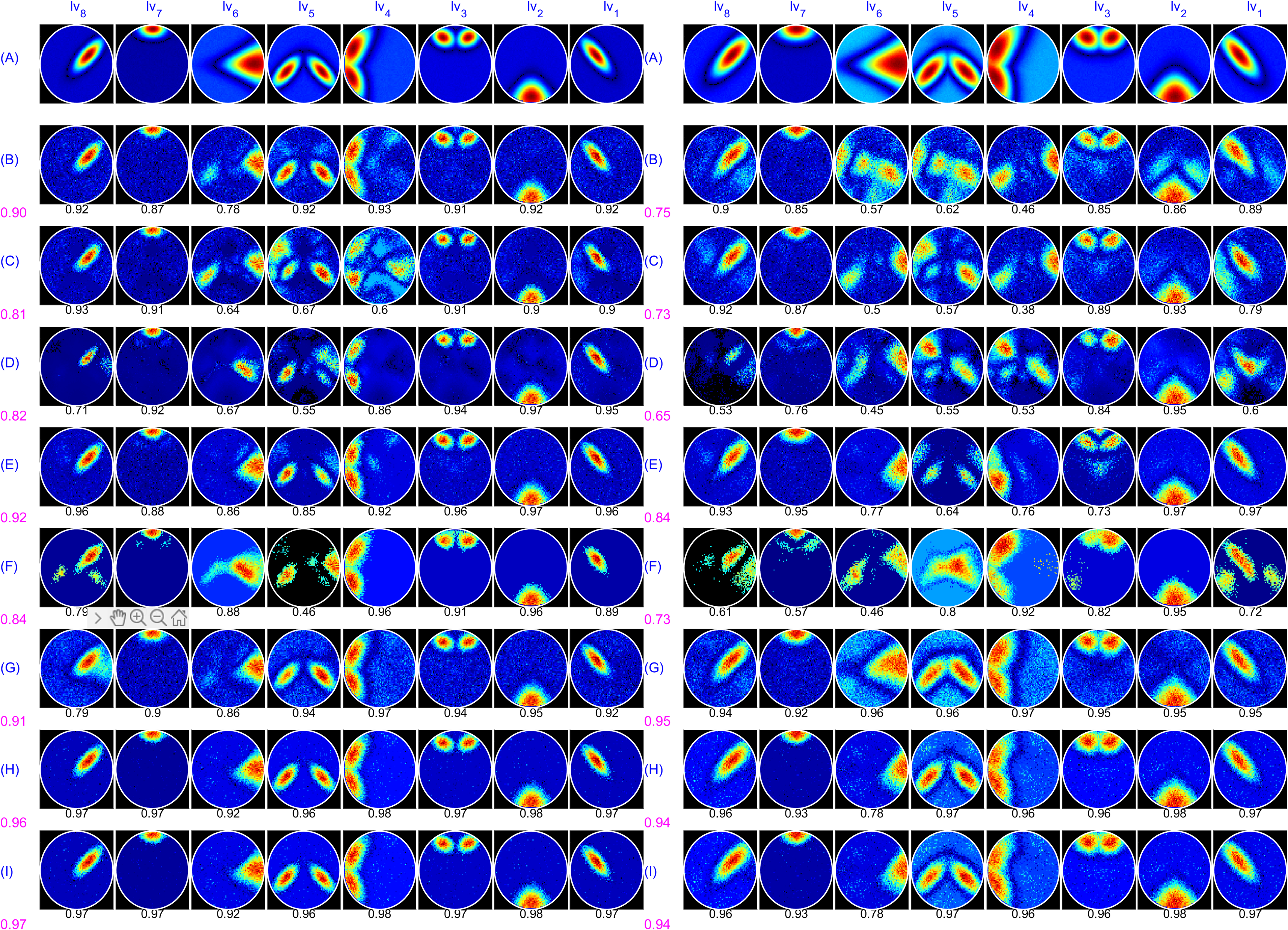
Figure 1: Row (A) displays the ground truth spatial maps with moderate (left, $\rho=6$) and significant (right, $\rho=12$) overlaps. Rows (B) through (I) show the maps recovered as loading vectors/sources by various algorithms including B) PCA+ICA, C) PPCA+ICA, D) SPCA+ICA, E) PMD, F) GPower, G) DPCA1a, H) DPCA1b, and I) DPCA2. Correlation values between the ground truth and the recovered sources are indicated for each map, with the mean correlation displayed on the left.

II-A Simulation study

II-A1 Synthetic dataset generation

The Simtb toolbox [37] was utilized to create a synthetic dataset that mimics the characteristics of experimental fMRI signals, which are distinguished by their sparse characteristics [38]. Using this toolbox, eight distinct PCs and LVs were created. Each PC consisted of $240$ data points that were taken from discrete cosine transform with bases numbers $\{3,11,19,27,35,43,51,59\}$, and each loading vector was represented by a $70\times 70$ voxel square image. All PCs were normalized to have zero mean and a variance of one. The LVs were created using these source identifiers $\{30,6,2,20,9,23,11,29\}$. Image slice activations were produced by deploying Gaussian distributions defined by parameters for position, orientation, and spread. The spatial coverage of these activations was regulated through the spread parameter ($\rho$), represented by Gaussian distribution as $\sim\mathcal{N}(\rho,\,0.05)$.

The LVs with two different i) moderate (left), and ii) significant (right) spatial overlaps are shown in Figure 1A, which are also considered as the ground truth (GT) LVs when retrieving the underlying spatial sources. The GT-PCs and LVs were used to construct a synthetic data matrix through a linear mixture model defined as $\text{X}=\sum_{i=1}^{8}(\text{pc}_{i}+\omega_{i})(\text{lv}^{i}+\gamma^{i})$. In this model, the noise matrices $\Omega\in\mathbb{R}^{240\times 8}$ and $\Gamma\in\mathbb{R}^{8\times 4900}$ were generated from Gaussian distributions, specifically $\Omega\sim\mathcal{N}(0,\,\eta_{t})$ and $\Gamma\sim\mathcal{N}(0,\,\eta_{s})$, where $\eta_{t}$ and $\eta_{s}$ are temporal and spatial noise variances, respectively. The matrix $\text{PC}\in\mathbb{R}^{240\times 8}$ represents the time courses, and $\text{LV}\in\mathbb{R}^{8\times 4900}$ contains the spatial maps obtained by reshaping the image slices. The synthetic dataset X was created based on the spread parameter $\rho$, spatial noise $\eta_{s}$, and temporal noise $\eta_{t}$, and subsequently used for source retrieval across all participating algorithms.

II-A2 Synthetic dataset configuration and parameters

Various algorithms were assessed to understand their effectiveness in data recovery. For instance, traditional PCA combined with spatial ICA (PCA+ICA) did not enhance interpretability nor did it effectively recover underlying sources, particularly in cases with considerable spatial overlaps. While PPCA+ICA marginally improved interpretability by leveraging sparse components, it was still inadequate for robust source separation. SPCA integrated with ICA (SPCA+ICA) also underperformed, particularly with significant spatial overlaps. These observations underscore the limitations of combining PCA with ICA and highlight the necessity for the proposed algorithms, which aim to simultaneously boost interpretability and ensure effective source separation.

For all algorithms, eight components were extracted. The sparsity parameter for each algorithm was selected based on optimal performance measures, such as the correlation between retrieved components and generated sources. For PPCA, the sparsity parameter was set to $0.005$. The sparsity parameter for SPCA was chosen according to the ground truth, which corresponds to the number of active pixels in the source slices. For PMD, the sparsity parameter was set to $0.43$, and for GPower, it was determined to be $0.3$. For the proposed algorithms, the sparsity parameter was normalized using a factor based on the data matrix dimensions, specifically $\sqrt{n\times p}$. This resulted in a sparsity parameter of $\lambda=0.67$ for all proposed algorithms, with $\rho_{1}=0.12$ and $\rho_{2}=0.24$ for DPCA1b and DPCA2. The proposed algorithms and PPCA were run for $30$ iterations, while the default iteration settings were used for all other algorithms.

TABLE IV: The average correlation values for the eight loading vectors ($lv_{1}$–$lv_{8}$) over 15 trials are presented, along with the mean and standard deviation (Std) for each algorithm. The highest and second-highest values are highlighted in bold.

Algos	$lv_{1}$	$lv_{2}$	$lv_{3}$	$lv_{4}$	$lv_{5}$	$lv_{6}$	$lv_{7}$	$lv_{8}$	Mean	Std
PCA+ICA	0.909	0.932	0.919	0.779	0.810	0.720	0.870	0.919	0.857	0.048
PPCA+ICA	0.899	0.914	0.922	0.608	0.696	0.649	0.906	0.930	0.816	0.028
SPCA+ICA	0.916	0.960	0.924	0.846	0.582	0.598	0.913	0.763	0.813	0.037
PMD	0.949	0.970	0.930	0.911	0.887	0.850	0.914	0.947	0.920	0.026
GPower	0.884	0.957	0.898	0.951	0.601	0.847	0.856	0.824	0.852	0.056
DPCA1a	0.926	0.947	0.942	0.967	0.879	0.819	0.893	0.867	0.905	0.032
DPCA1b	0.967	0.978	0.972	0.979	0.911	0.799	0.966	0.967	0.942	0.019
DPCA2	0.967	0.978	0.973	0.979	0.899	0.787	0.965	0.968	0.939	0.020

II-A3 Synthetic dataset results

The results in Figure 1 demonstrate the effectiveness of eight algorithms (B to I) in recovering ground truth spatial maps (LVs) from a generated dataset X. The top row (A) shows the ground truth LVs under two conditions: moderate spatial overlap on the left and significant spatial overlap on the right. This ground truth, along with setting $\eta_{t}=0.9$ and $\eta_{s}=0.005$, was used to generate the data matrix X according to the discussion in the previous subsection. Each recovered map has an associated correlation value, reflecting its similarity to the ground truth. Higher correlation values indicate better recovery. The magenta values on the left represent the mean correlation for each algorithm, providing an overall performance metric.

In the moderate overlap scenario, most algorithms performed well, with the proposed algorithms (G, H, I), PCA+ICA, and PMD achieving particularly high correlations, indicating accurate recovery. However, in situations with significant overlap, performance declined for some methods, especially PCA+ICA, PPCA+ICA, and SPCA+ICA which struggled to recover ground truth accurately. This suggested that combining PCA with ICA may not be sufficient for such complex scenarios, and SPCA+ICA was even worst than PCA+ICA, thus supporting the proposed hypothesis. GPower also showed lower correlation values, while PMD performed better but still fell short of the proposed algorithms.

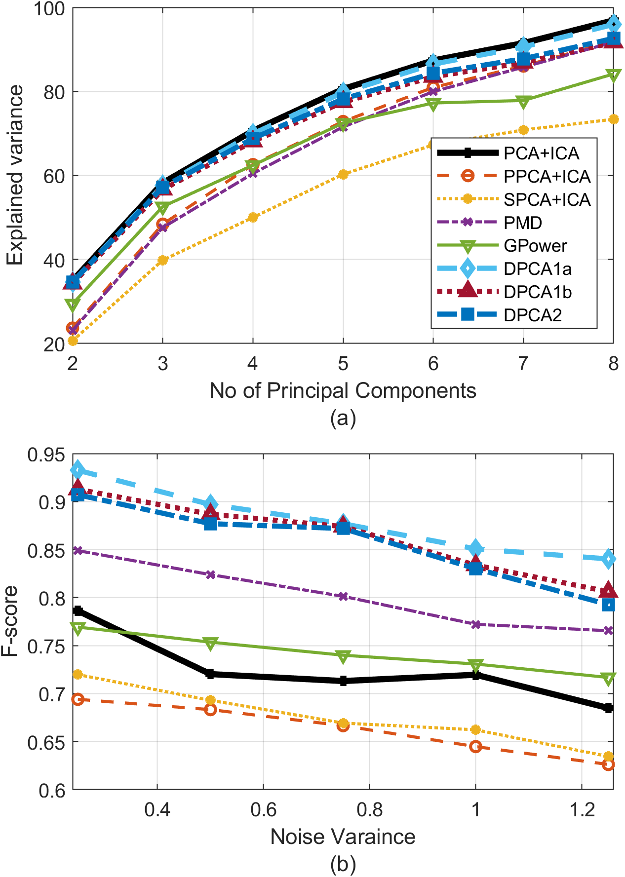
Figure 2: a) Comparison of all algorithms on synthetic data to illustrate the variance explained as the number of principal components varied from $2$ to $8$, and b) mean F-score over $10$ trials calculated for various noise variances across all algorithms.

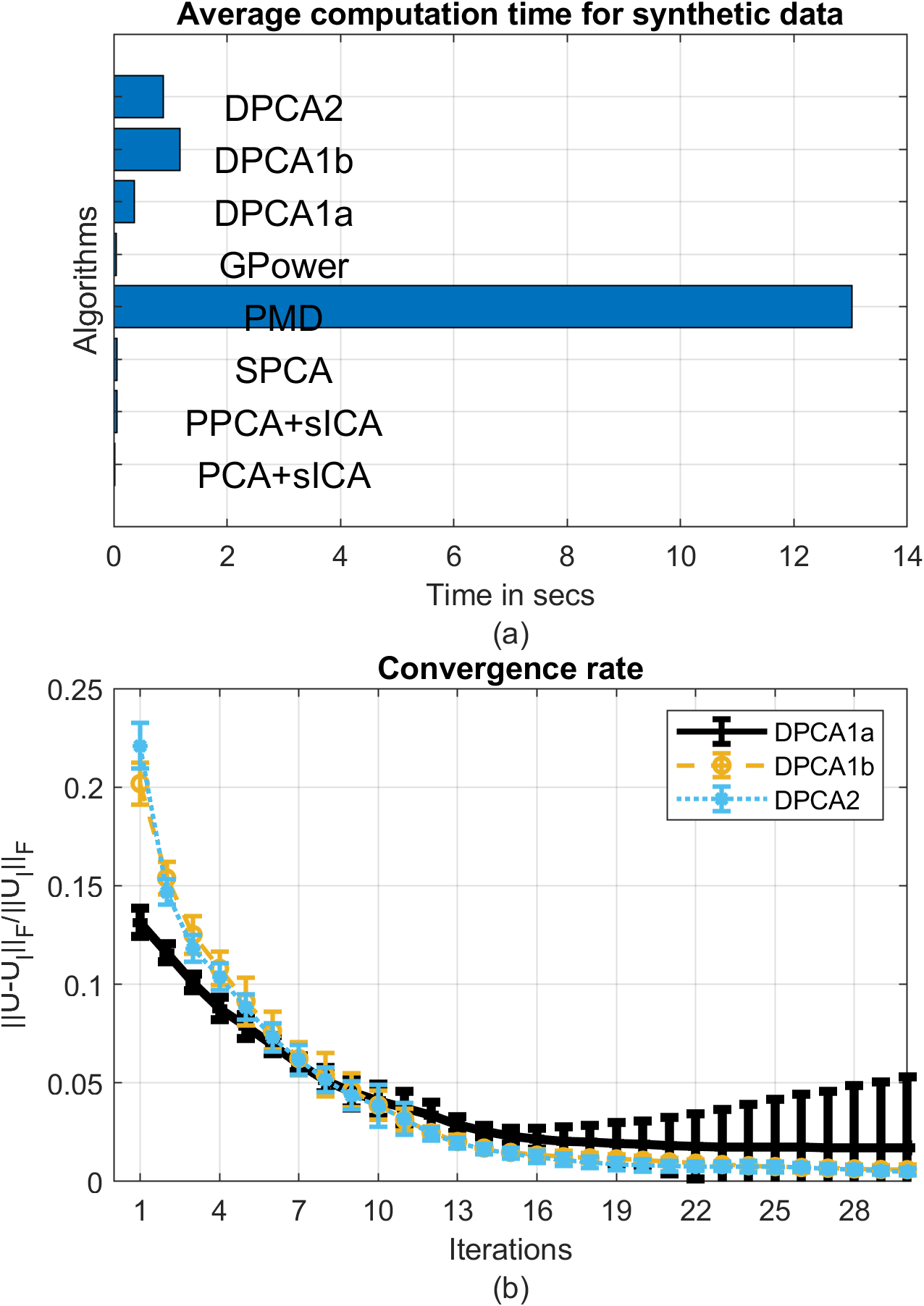
Figure 3: a) Average computation time illustrating the time efficiency of various algorithms when processing synthetic data, and b) convergence rate displaying the convergence behavior of the DPCA variants, measured by the normalized difference between successive updates along with error bars indicating variability across runs.

For each algorithm, the experiment from Figure 1 was repeated $15$ times with temporal noise variance set to $0.9$ and spatial noise variance set to $0.005$, and spread parameter set to $6$. The results in Table IV show the mean correlation values for each loading vector ($lv_{1}-lv_{8}$), along with the overall mean and standard deviation for each algorithm. PPCA+ICA and SPCA+ICA produced the lowest mean correlations compared to other algorithms, while PCA+ICA and GPower achieved slightly higher means but with greater variability. PMD performed better, with a mean correlation of $0.920$ and a moderate standard deviation of $0.026$. The DPCA variants (DPCA1b and DPCA2) stood out, showing the highest mean correlations and lowest standard deviations, indicating superior consistency and accuracy. This indicates that DPCA1b and DPCA2 excel in accurately recovering GT-LVs, showing superior performance compared to traditional combinations of PCA and ICA.

Figure 2 compares several algorithms on synthetic data, focusing on explained variance and mean F-score under varying noise conditions. In subfigure (a), the explained variance is shown, as the number of PCs increased from $2$ to $8$, with temporal and spatial noise variances set to $0.3$ and $0.005$, and a spread parameter of $8$. The DPCA variants (DPCA1a, DPCA1b, and DPCA2) collectively achieved the second highest explained variance across all component settings, demonstrating their superior ability to capture data variance. GPower, and PMD showed moderate performance, while PCA+ICA and DPCA1a reached the highest explained variance levels among all algorithms.

Figure 2b presents the mean F-scores over $10$ trials for each algorithm across varying noise levels, with temporal noise ranging from $0.25$ to $1.2$ and spatial noise from $0.001$ to $0.017$, while spread parameter set to $8$. The DPCA1a consistently achieved the highest F-scores, while DPCA1b and DPCA2 followed closely, demonstrating robust and accurate source recovery even in high noise environments. In contrast, the combination methods SPCA+ICA and PPCA+ICA displayed a rapid decline in F-scores as noise increased, signaling decreased effectiveness. Meanwhile, PMD and GPower exhibited a moderate decline but generally lower F-scores, underscoring less robustness compared to the DPCA variants.

Figure 3 illustrates a comprehensive performance comparison of various decomposition algorithms under different noise conditions, extracted from a scenario where temporal and spatial noise levels were systematically varied as shown in Figure 2b. In subfigure (a), the average computation time for each algorithm is charted, revealing the DPCA variants, particularly DPCA1b, as the most computationally demanding. Figure 3b depicts the convergence rates of the DPCA variants. Each line indicates a consistent decrease in error as the iterations progress, which highlights the effectiveness of these algorithms (DPCA1b and DPCA2) in converging to a stable solution efficiently. Error bars indicate variability in convergence rates across trials, highlighting the stability of each algorithm under various data conditions. These insights reveal that DPCA1a experiences issues with convergence.

III Image Applications

III-A Background subtraction on video sequences

TABLE V: For all algorithms involved in background subtraction, the sparsity parameters and computation time in seconds are reported as ${\lambda,\rho_{1},\rho_{2},\text{seconds}}$. The lowest computation time is highlighted in bold.

Dataset	SPCA	PMD	GPower	DPCA1a	DPCA1b	DPCA2
Highway traffic	300,4.5	0.45,2.1	0.3,2.3	190,11.4	190,4,16,5.3	190,4,16,15.7
People in a corridor	250,1.7	0.45,1.3	0.01,2.4	600,3.8	600,12,32,1.2	1600,12,32,8.2
Person crossing a street	390,5.0	0.6,2.9	0.1,2.3	60,27.2	60,3,9,4.5	60,3,9,14.3

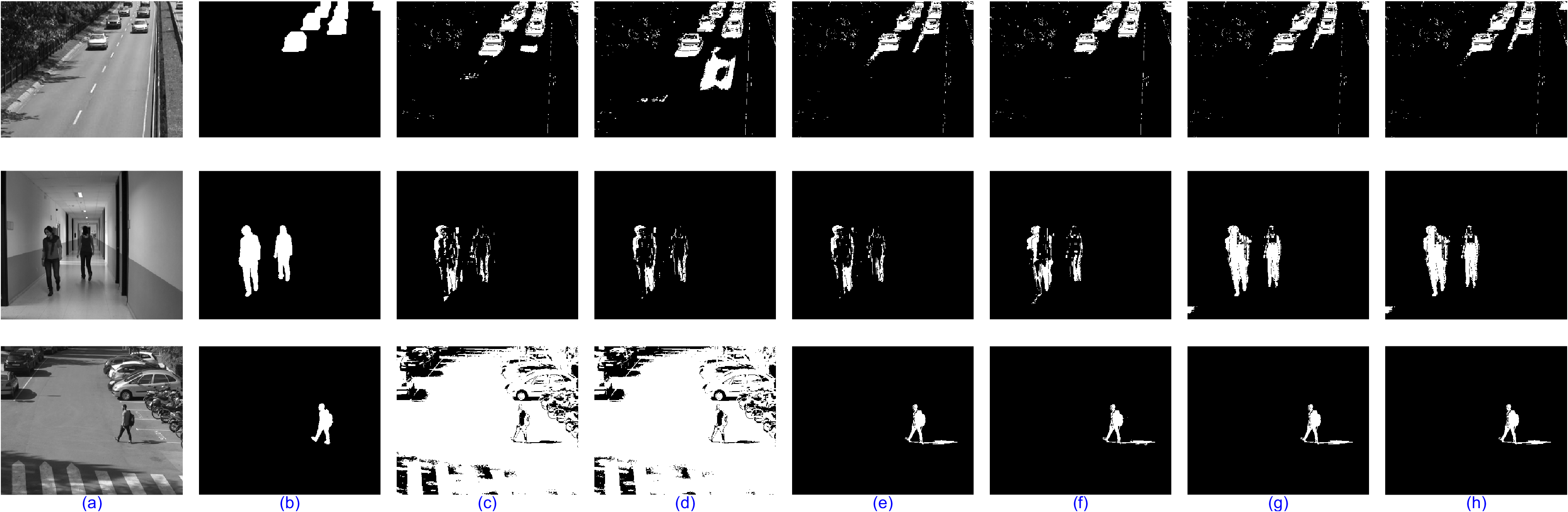
Figure 4: a) shows the original images from three distinct scenarios: highway traffic, people in a corridor, and a person crossing a street. b) displays the ground truth for foreground detection, (c) through (i) display the foregrounds recovered by various algorithms in the following order: SPCA, PMD, GPower, DPCA1a, DPCA1b, and DPCA2, each corresponding to the scenarios depicted.

In this section, the performance of the proposed algorithms was evaluated through the application of background subtraction. This technique processed a video sequence, utilizing the frames to train ten PCs and their corresponding LVs which effectively model the background. Subsequently, pixels that significantly deviate from this decomposition model are identified as foreground. This method allows for dynamic separation of background and foreground elements, crucial for various video processing applications. This problem has been formulated as a sparse signal recovery problem in prior studies [39, 40, 41, 42], employing a data decomposition model denoted as $\text{X}=\text{U}\text{Z}$. This model facilitates the decomposition of vectorized video sequences stored in X into PCs represented by matrix U and their corresponding LVs contained within Z. After extracting the LVs, the background for each frame $\tilde{\text{x}}_{i}$ is reconstructed using a linear combination of PCs from the matrix U and the sparse loading vector $\text{z}_{i}$, as $\tilde{\text{x}}_{i}=\text{U}\text{z}_{i}$. The foreground for each frame is then determined by calculating the residual $\text{x}_{i}-\tilde{\text{x}}_{i}$.

Three grayscale video sequences were considered from two different databases to make the evaluation diverse. This included a highway sequence from CDnet-2014 dataset, a bootstrap sequence and a person crossing a street from LASIESTA dataset. The first sequence is of a of highway traffic that displays a fair number of foreground objects, appearing as medium traffic density in some frames and light traffic in others. The second sequence features two foreground objects consisting of two people walking in a corridor who shake hands in some frames and walk in opposite directions in others. The third sequence showcases a person crossing a street in a sunny area, while in later frames, another person crosses in the opposite direction in a shaded area.

The highway traffic video sequence has dimensions of $240\times 320$ pixels across $1700$ frames. For evaluation purposes, only a subset of $400$ frames (from frame $700$ to $1099$) was utilized. The video of people in the corridor has dimensions of $288\times 352$ pixels over $275$ frames, and the video of a person crossing the street comprises $288\times 352$ pixels across $400$ frames. In all sequences, the camera position was static. Each frame was vectorized to form the columns of the data matrix X.

Only algorithms that demonstrated competitive performance were selected for this study, specifically SPCA, PMD, GPower, and the newly proposed algorithms. I configured each algorithm to extract $10$ PCs and iterated the proposed algorithms for $20$ cycles. Default iteration settings were applied to the other algorithms. The optimal sparsity parameter for each algorithm was determined by experimenting with various values and selecting the one that yielded the highest F-score. Details of these sparsity parameters and the computation times for each algorithm are provided in Table V.

After extracting components, a query image from each video sequence was selected to retrieve its corresponding trained foreground and background. The original query images, their ground truths, and the thresholded recovered foregrounds are presented in Figure 4. Overall, DPCA1a, DPCA1b, DPCA2, and GPower demonstrate more precise and accurate foreground detections across varied scenarios compared to SPCA and PMD. These latter algorithms struggle with consistency in complex scenes that feature multiple elements and variable lighting. Specifically, the DPCA variants excelled by accurately capturing most vehicles in the first dataset, providing clear and distinct outlines of individuals in the second dataset, and precisely capturing the silhouette of the person in the third dataset.

Table VI, quantitatively evaluates the performance of six distinct algorithms by measuring precision, recall, and F-score across three varied scenarios. These results are correlated with the visual outcomes illustrated in Figure 4. The data reveals that while SPCA and PMD provide useful insights, their performance fluctuates in complex settings. In contrast, the DPCA variants and GPower demonstrate consistently superior precision and F-scores, indicating not only higher accuracy but also robustness in handling diverse foreground extraction challenges effectively.

TABLE VI: Precision, Recall and F-score for the results shown in Figure 4 using six different algorithms.

Algorithm	Highway traffic			People in a corridor			Person crossing a street
	Preci.	Recall	F-score	Preci.	Recall	F-score	Preci.	Recall	F-score
SPCA	0.725	0.700	0.712	0.541	0.239	0.331	0.012	0.667	0.023
PMD	0.443	0.660	0.530	0.644	0.239	0.348	0.011	0.644	0.022
GPower	0.804	0.677	0.735	0.685	0.256	0.372	0.780	0.757	0.768
DPCA1a	0.807	0.713	0.757	0.733	0.368	0.490	0.785	0.756	0.771
DPCA1b	0.830	0.692	0.755	0.828	0.776	0.801	0.782	0.756	0.770
DPCA2	0.817	0.691	0.749	0.825	0.778	0.803	0.782	0.757	0.769

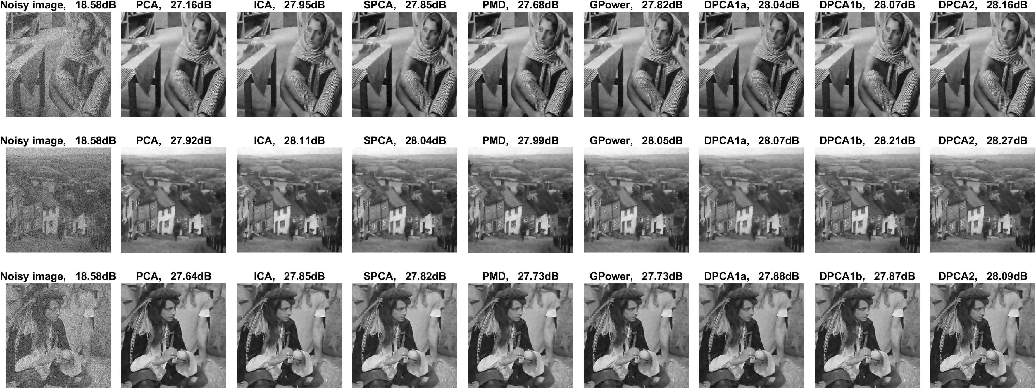
Figure 5: The first column display the original noisy images with an input PSNR of 18.58dB. Subsequent images illustrate the results of image reconstruction using eight different methods: PCA, ICA, SPCA, PMD, GPower, DPCA1a, DPCA1b, and DPCA2. Output PSNR values are noted above each image, demonstrating the effectiveness of each reconstruction technique across three distinct images: Barbara, Hill, and Man.

III-B Image reconstruction

This section evaluates the image reconstruction capabilities of the proposed algorithms against established methods including PCA, ICA, SPCA, PMD, and GPower. The test images were sourced from the miscellaneous category of the SIPI image database [43]. Each original image, sized $512\times 512$, was converted to grayscale with pixel values ranging from $0$ to $255$. To simulate real-world conditions, Gaussian noise was added to these clean images. The noisy versions were then processed to create a training dataset. This was done by extracting $20000$ overlapping $8\times 8$ patches using a sliding neighborhood approach, vectorizing these patches, removing their mean, and assembling them into the columns of the training matrix $\text{X}\in\mathbb{R}^{64\times 20000}$ [27, 44].

Only algorithms that demonstrated competitive performance were included in this study including PCA, ICA, SPCA, PMD, GPower, and the newly proposed DPCA variants. Each algorithm was configured to extract $64$ PCs, with the proposed algorithms iterating through $20$ cycles. Default settings were maintained for other algorithms. The optimal sparsity parameter for each was determined through experimentation, selecting values that maximized the PSNR, as detailed in Table VII. After extracting the components, the denoised images were reconstructed by averaging pixels across all overlapping patches that had been processed for sparse representation [45].

In Figure 5, various image reconstruction techniques were applied to three different noisy images (Barbara, Hill, and Man), and their performance is quantified using the PSNR metric. PCA typically showed moderate improvement over the noisy input across all images. SPCA offered varying results, while it performed better on the Hill image, indicating some scenarios where the method may capture underlying structures effectively. ICA consistently provided a notable improvement in PSNR compared to PCA and SPCA. PMD displayed performance comparable to SPCA, highlighting its potential in scenarios where subtle textural features need to be preserve, but its computational inefficiency was quite high. GPower demonstrated strong performance across all images. DPCA variants (DPCA1a, DPCA1b, and DPCA2) consistently achieved the highest PSNR values among all algorithms. This indicates that these methods are particularly effective in handling noise and preserving or enhancing image details.

Table VIII considers scenarios with even higher noise variance. It revealed that DPCA variants consistently outperform traditional methods like PCA, ICA, and SPCA across all images, demonstrating superior noise reduction capabilities while preserving image details. DPCA2 in particular often achieved the highest PSNR values, notably with the Hill and Man images, illustrating its effectiveness in managing various noise levels and image complexities. This highlights the advantages of integrating DMs and adaptive thresholding techniques in image reconstruction.

TABLE VII: For some of the algorithms involved in image reconstruction, the sparsity parameters are reported as ${\lambda,\rho_{1},\rho_{2}}$.

Images	PSNRin	SPCA	PMD	GPower	DPCA1a	DPCA1b	DPCA2
Barbara	18.58	30	0.40	0.20	9000	9000,15,50	9000,15,50
	14.14	40	0.45	0.15	50000	50000,10,45	50000,10,45
	11.22	30	0.41	0.25	64000	64000,10,45	64000,10,45
Hill	18.58	30	0.40	0.20	8000	9000,10,40	9000,10,40
	14.14	40	0.45	0.15	32000	32000,10,45	32000,10,45
	11.22	30	0.41	0.25	64000	64000,10,45	64000,10,45
Man	18.58	30	0.40	0.20	9000	9000,15,50	9000,15,50
	14.14	40	0.45	0.15	32000	32000,10,45	32000,10,45
	11.22	30	0.41	0.25	64000	64000,10,45	64000,10,45

III-C Image inpainting

In this section, the evaluation of the proposed algorithms is conducted through image inpainting tasks aimed at recovering missing pixels caused by superimposed text. The training dataset X was composed of $1000$ randomly selected $8\times 8$ patches from nine images sourced from the miscellaneous category of the SIPI image database [43]. All algorithms were then applied to this training set, which has dimensions of $64\times 9000$, to extract PCs sized $64\times 64$. Whereas two testing images were selected from this database, whiche were first painted using a text mask, and then divided into $N$ overlapping patches to produce an image matrix B of size $64\times N$, where $N=62000$. Only algorithms that demonstrated competitive performance were selected for this study, specifically DCT bases of size $64\times 256$, PCA, DPCA1a, DPCA1b, DPCA2. All algorithms were run for $10$ iterations, and the best performing sparsity parameter was determined through extensive testing for each algorithm, and was found to be $\{\lambda,\rho_{1},\rho_{2}\}=\{3000,10,40\}$ for the pepper’s image and $\{3000,10,40\}$ for the couple’s image.

The Orthogonal Matching Pursuit (OMP) sparse coding technique was employed to learn sparse coefficients for each vector in B, aiming to minimize the reconstruction error $\left\lVert\text{M}\circ(\text{b}_{i}-\text{U}\text{z}_{i})\right\rVert{F}^{2}$ for $i={1,...,N}$, where $\circ$ denotes element-wise multiplication, and M represents the mask indicating missing pixels. The sparsity parameter was uniformly set to $20$ across all algorithms for both test images. The outcomes, displayed in Figure 6, were quantified using the PSNR and the sum of squared errors (SSE) between the original and reconstructed images. Notably, the DPCA2 algorithm excelled in reconstructing the pepper image with minimal text overlay, achieving the highest image quality. Similarly, for the more challenging case with a greater number of missing pixels, DPCA2 again, outperformed all other algorithms.

In conclusion, the DPCA variants, particularly DPCA1b and DPCA2, demonstrate superior recovery capabilities in both scenarios, efficiently restoring images with substantial text-induced damage. These algorithms notably outperform traditional PCA and DCT bases, affirming the effectiveness of advanced sparse coding and integrating dissociation matrices in complex inpainting tasks.

TABLE VIII: PSNR values in dB of noisy and denoised images recovered by seven diferent algorithms with best results highlighted in bold.

Images	PSNRin	PCA	ICA	SPCA	GPower	DPCA1a	DPCA1b	DPCA2
Barbara	14.14	24.400	24.966	24.916	24.915	25.229	25.232	25.229
	11.22	22.871	23.102	23.136	23.130	23.331	23.362	23.386
Hill	14.14	26.087	26.164	26.165	26.180	26.246	26.214	26.282
	11.22	25.081	25.088	25.105	25.123	25.150	25.139	25.162
Man	14.14	25.582	25.663	25.675	25.643	25.772	25.788	25.906
	11.22	24.442	24.474	24.485	24.506	24.574	24.607	24.654
Mean		24.744	24.909	24.914	24.916	25.050	25.057	25.103

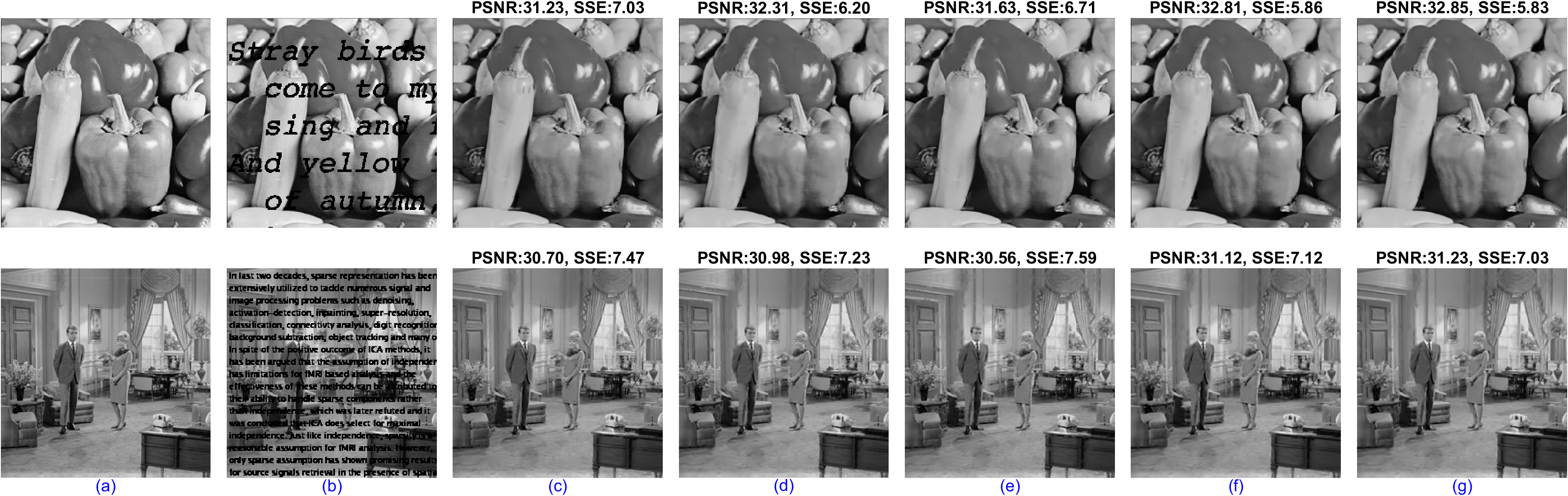
Figure 6: Image inpainting performance for two distinct scenarios: Peppers (top) and Couple (bottom). (a) shows the original images, (b) displays the images with text-overlay induced missing pixels, and (c) through (g) present the reconstructed images using DCT bases, PCA, DPCA1a, DPCA1b, and DPCA2, respectively. The performance of each reconstruction method is quantified by the PSNR and SSE values noted above each image.

IV Conclusion

The proposed algorithms significantly enhance source separation and interpretability in PCA by incorporating sequential component estimation and interdependency integration through dissociation matrices (DMs). This approach improves upon traditional sparse PCA by providing robust performance even in scenarios with significant spatial overlaps. The superiority of the DPCA1 and DPCA2 algorithms over traditional techniques like SPCA and ICA is shown by their testing and comparison across a range of applications. In conclusion, the DPCA framework is a substantial advancement in the analytical power of PCA approaches, offering practitioners and researchers a strong instrument for deriving insightful information from complex, high-dimensional datasets. Future work will aim to optimize these algorithms further and explore their potential across different datasets and applications, potentially incorporating advanced decomposition techniques such as deploying singular spectrum analysis [46] and empirical mode decomposition [47] for a second level decomposition [48] to obtain deeper insights.

References

- [1] K. Pearson, “LIII. On lines and planes of closest fit to systems of points in space,” The London, Edinburgh, and Dublin Philosophical Magazine and Journal of Science, vol. 2, no. 11, pp. 559–572, 1901.
- [2] I. Koch, Analysis of Multivariate and High-Dimensional Data, ser. Cambridge Series in Statistical and Probabilistic Mathematics. Cambridge: Cambridge University Press, 2013.
- [3] H. Hotelling, “Analysis of a complex of statistical variables into principal components,” Journal of Educational Psychology, vol. 24, no. 6, pp. 417–441, 1933.
- [4] G. W. Stewart, “On the Early History of the Singular Value Decomposition,” SIAM Rev., vol. 35, no. 4, pp. 551–566, Dec. 1993.
- [5] I. T. Jolliffe and J. Cadima, “Principal component analysis: A review and recent developments,” Philosophical Transactions of the Royal Society A: Mathematical, Physical and Engineering Sciences, vol. 374, no. 2065, p. 20150202, Apr. 2016.
- [6] A.-K. Seghouane, N. Shokouhi, and I. Koch, “Sparse Principal Component Analysis With Preserved Sparsity Pattern,” IEEE Transactions on Image Processing, vol. 28, no. 7, pp. 3274–3285, Jul. 2019.
- [7] O. Friman, M. Borga, P. Lundberg, and H. Knutsson, “Exploratory fMRI analysis by autocorrelation maximization,” Neuroimage, vol. 16, no. 2, pp. 454–464, Jun. 2002.
- [8] J. N. R. Jeffers, “Two Case Studies in the Application of Principal Component Analysis,” Journal of the Royal Statistical Society. Series C (Applied Statistics), vol. 16, no. 3, pp. 225–236, 1967.
- [9] H. Zou and L. Xue, “A Selective Overview of Sparse Principal Component Analysis,” Proceedings of the IEEE, vol. 106, pp. 1311–1320, 2018.
- [10] A. M. Tillmann and M. E. Pfetsch, “The Computational Complexity of the Restricted Isometry Property, the Nullspace Property, and Related Concepts in Compressed Sensing,” IEEE Transactions on Information Theory, vol. 60, no. 2, pp. 1248–1259, Feb. 2014.
- [11] T. Wang, Q. Berthet, and R. J. Samworth, “Statistical and Computational Trade-Offs in Estimation of Sparse Principal Components,” The Annals of Statistics, vol. 44, no. 5, pp. 1896–1930, 2016.
- [12] R. Guerra-Urzola, K. Van Deun, J. C. Vera, and K. Sijtsma, “A Guide for Sparse PCA: Model Comparison and Applications,” Psychometrika, vol. 86, no. 4, pp. 893–919, Dec. 2021.
- [13] I. T. Jolliffe, N. T. Trendafilov, and M. Uddin, “A Modified Principal Component Technique Based on the LASSO,” Journal of Computational and Graphical Statistics, vol. 12, no. 3, pp. 531–547, Sep. 2003.
- [14] H. Zou, T. Hastie, and R. Tibshirani, “Sparse Principal Component Analysis,” Journal of Computational and Graphical Statistics, vol. 15, no. 2, pp. 265–286, 2006.
- [15] A. d’Aspremont, L. E. Ghaoui, M. I. Jordan, and G. R. G. Lanckriet, “A Direct Formulation for Sparse PCA Using Semidefinite Programming,” SIAM Review, vol. 49, no. 3, pp. 434–448, 2007.
- [16] D. M. Witten, R. Tibshirani, and T. Hastie, “A penalized matrix decomposition, with applications to sparse principal components and canonical correlation analysis,” Biostatistics, vol. 10, no. 3, pp. 515–534, 2009.
- [17] Z. Ma, “Sparse principal component analysis and iterative thresholding,” The Annals of Statistics, vol. 41, no. 2, pp. 772–801, Apr. 2013.
- [18] M. Journée, Y. Nesterov, P. Richtárik, and R. Sepulchre, “Generalized Power Method for Sparse Principal Component Analysis,” J. Mach. Learn. Res., vol. 11, pp. 517–553, Mar. 2010.
- [19] X.-T. Yuan and T. Zhang, “Truncated power method for sparse eigenvalue problems,” J. Mach. Learn. Res., vol. 14, pp. 899–925, 2013.
- [20] P.-A. Mattei, C. Bouveyron, and P. Latouche, “Globally Sparse Probabilistic PCA,” in Proceedings of the 19th International Conference on Artificial Intelligence and Statistics. PMLR, May 2016. ISSN 1938-7228 pp. 976–984.
- [21] Y. Qiu, J. Lei, and K. Roeder, “Gradient-based sparse principal component analysis with extensions to online learning,” Biometrika, vol. 110, no. 2, pp. 339–360, Jun. 2023.
- [22] F. Chen and K. Rohe, “A New Basis for Sparse Principal Component Analysis,” Journal of Computational and Graphical Statistics, vol. 33, no. 2, pp. 421–434, Apr. 2024.
- [23] M. U. Khalid and A.-K. Seghouane, “Unsupervised detrending technique using sparse dictionary learning for fMRI preprocessing and analysis,” in 2015 IEEE International Conference on Acoustics, Speech and Signal Processing (ICASSP), Apr. 2015, pp. 917–921.
- [24] A.-K. Seghouane and M. U. Khalid, “Learning dictionaries from correlated data: Application to fMRI data analysis,” in IEEE International Conference on Image Processing (ICIP), 2016, pp. 2340–2344.
- [25] W. Zhang, J. Lv, X. Li, D. Zhu, X. Jiang, S. Zhang, Y. Zhao, L. Guo, J. Ye, D. Hu, and T. Liu, “Experimental Comparisons of Sparse Dictionary Learning and Independent Component Analysis for Brain Network Inference From fMRI Data,” IEEE Trans Biomed Eng, vol. 66, no. 1, pp. 289–299, Jan. 2019.
- [26] I. T. Jolliffe, Principal Component Analysis for Special Types of Data. Springer, 2002.
- [27] M. Aharon, M. Elad, and A. Bruckstein, “K-SVD: An algorithm for designing overcomplete dictionaries for sparse representation,” IEEE Transactions on Signal Processing, vol. 54, no. 11, pp. 4311–4322, 2006.
- [28] F. Chen, S. Roch, K. Rohe, and S. Yu, “Estimating Graph Dimension with Cross-validated Eigenvalues,” 2021.
- [29] H. Shen and J. Z. Huang, “Sparse principal component analysis via regularized low rank matrix approximation,” Journal of Multivariate Analysis, vol. 99, no. 6, pp. 1015–1034, Jul. 2008.
- [30] S. Park, E. Ceulemans, and K. Van Deun, “A critical assessment of sparse PCA (research): Why (one should acknowledge that) weights are not loadings,” Behav Res Methods, vol. 56, pp. 1413–1432, 2024.
- [31] H. Zou, “The Adaptive Lasso and Its Oracle Properties,” Journal of the American Statistical Association, vol. 101, pp. 1418–1429, 2006.
- [32] S. Voronin and R. Chartrand, “A New Generalized Thresholding Algorithm for Inverse Problems with Sparsity Constraints,” in ICASSP, IEEE International Conference on Acoustics, Speech and Signal Processing - Proceedings, Oct. 2013. doi: 10.1109/ICASSP.2013.6637929
- [33] A.-K. Seghouane and A. Iqbal, “Consistent adaptive sequential dictionary learning,” Signal Processing, vol. 153, pp. 300–310, Dec. 2018.
- [34] W. J. Fu, “Penalized Regressions: The Bridge versus the Lasso,” Journal of Computational and Graphical Statistics, vol. 7, pp. 397–416, 1998.
- [35] J. Mairal, F. Bach, J. Ponce, and G. Sapiro, “Online dictionary learning for sparse coding,” in Proceedings of the 26th Annual International Conference on Machine Learning, ser. ICML ’09. New York, NY, USA: Association for Computing Machinery, Jun. 2009, pp. 689–696.
- [36] D. P. Bertsekas, Nonlinear Programming, 3rd ed. Belmont, Mass: Athena Scientific, Jun. 2016. ISBN 978-1-886529-05-2
- [37] E. Erhardt, E. Allen, Y. Wei, T. Eichele, and V. Calhoun, “SimTB, a simulation toolbox for fMRI data under a model of spatiotemporal separability,” NeuroImage, vol. 59, pp. 4160–7, Dec. 2011.
- [38] A.-K. Seghouane and M. U. Khalid, “Hierarchical sparse brain network estimation,” in 2012 IEEE International Workshop on Machine Learning for Signal Processing, Sep. 2012, pp. 1–6.
- [39] J. Huang, X. Huang, and D. Metaxas, “Learning with dynamic group sparsity,” in 2009 IEEE 12th International Conference on Computer Vision, Sep. 2009. ISSN 2380-7504 pp. 64–71.
- [40] C. Lu, J. Shi, and J. Jia, “Online Robust Dictionary Learning,” in 2013 IEEE Conference on Computer Vision and Pattern Recognition, Jun. 2013. doi: 10.1109/CVPR.2013.60. ISSN 1063-6919 pp. 415–422.
- [41] A. Iqbal and A.-K. Seghouane, “Robust Dictionary Learning Using -Divergence,” in ICASSP 2019 - 2019 IEEE International Conference on Acoustics, Speech and Signal Processing (ICASSP), May 2019. doi: 10.1109/ICASSP.2019.8683210. ISSN 2379-190X pp. 2972–2976.
- [42] A. Miri Rekavandi, A.-K. Seghouane, and R. J. Evans, “Learning Robust and Sparse Principal Components With the -Divergence,” IEEE Trans Image Process, vol. 33, pp. 3441–3455, 2024.
- [43] “SIPI Image Database,” https://sipi.usc.edu/database/.
- [44] M. U. Khalid, A. Miri Rekavandi, A.-K. Seghouane, and M. Palaniswami, “Efficient Two-Dimensional Sparse Sequential Dictionary Learning Methods,” Rochester, NY, Jan. 2024.
- [45] P. Irofti and B. Dumitrescu, “Pairwise Approximate K-SVD,” in ICASSP 2019 - 2019 IEEE International Conference on Acoustics, Speech and Signal Processing (ICASSP), May 2019, pp. 3677–3681.
- [46] H. Hassani, “Singular Spectrum Analysis: Methodology and Comparison,” Journal of Data Science, vol. 5, no. 2, pp. 239–257, Aug. 2022.
- [47] D. Kim and H.-S. Oh, “EMD: A Package for Empirical Mode Decomposition and Hilbert Spectrum,” The R Journal, vol. 1, pp. 40–46, 2009.
- [48] M. U. Khalid, M. M. Nauman, S. Akram, and K. Ali, “Three layered sparse dictionary learning algorithm for enhancing the subject wise segregation of brain networks,” Sci Rep, vol. 14, p. 19070, 2024.