A pursuit problem for squared Bessel processes

Abstract.

In this note, we are interested in the probability that two independent squared Bessel processes do not cross for a long time. We show that this probability has a power decay which is given by the first zero of some hypergeometric function. We also compute along the way the distribution of the location where the crossing eventually occurs, as well as some Cramér’s estimates for squared Bessel processes perturbed by a power drift.

1. Introduction

1.1. Statement of the main result

Let $X$ and $Y$ be two independent squared Bessel processes of respective dimensions $\alpha>0$ and $\beta\geq 0$. We denote by $\mathbb{P}_{(x,y)}$ the law of the pair $(X,Y)$ when starting from $(x,y)$ and we assume that $0\leq x<y$. In this note, we are interested in the probability that the process $X$ remains below $Y$ for a long time :

$$\mathbb{P}_{(x,y)}\left(\forall s\leq t,\,X_{s}<Y_{s}\right)\qquad\text{as }t\rightarrow+\infty.$$

This question is often labelled in the literature as a capture or a pursuit problem. In most papers, the set-up is a Brownian one and the leading process is called a lamb or a prisoner, while its pursuers are wolves or policemen, see for instance [10, 12, 15] and the reference therein. One may also see this question as a persistence problem for the difference of two squared Bessel processes. Indeed, a natural way to study such question is to introduce the stopping time

$$T=\inf\{t\geq 0,\,X_{t}=Y_{t}\}$$

and study its tail asymptotics since $\mathbb{P}_{(x,y)}\left(\forall s\leq t,\,X_{s}<Y_{s}\right)=\mathbb{P}_{(x,y)}\left(T>t\right)$. Unlike the sum of squared Bessel processes, the difference is no longer Markovian and studying such asymptotics is thus more delicate. We refer to the two surveys [2, 5] for an extensive background on persistence probabilities, as well as their links with many physic phenomenons.

In order to state our results, let us define the hypergeometric function ${}_{2}F_{1}$ (see for instance [7, Chapter 9.1]):

$${}_{2}F_{1}\biggl{[}\genfrac{.}{.}{0.0pt}{}{a\quad b}{c};z\biggr{]}=\sum_{n=0}^{+\infty}\frac{(a)_{n}(b)_{n}}{(c)_{n}}\frac{z^{n}}{n!}$$

where $(a)_{0}=1$ and $(a)_{n}=a(a+1)\ldots(a+n-1)=\dfrac{\Gamma(a+n)}{\Gamma(a)}$ for $n\in\mathbb{N}$. We denote by $F_{\alpha,\beta}$ the hypergeometric function

$$F_{\alpha,\beta}(s)={}_{2}F_{1}\biggl{[}\genfrac{.}{.}{0.0pt}{}{\frac{\alpha+\beta}{2}-1+s\quad-s}{\frac{\alpha}{2}};\frac{1}{2}\biggr{]},\qquad s\geq 0.$$

Our first result gives the distribution of the position of $X$ and $Y$ when they cross each other.

Proposition 1.

Let us denote by $\theta$ the first positive zero of the hypergeometric function $F_{\alpha,\beta}$ :

$$\theta=\inf\left\{s\geq 0,\,F_{\alpha,\beta}(s)=0\right\}.$$

Under $\mathbb{P}_{(0,y)}$ the stopping time $T$ is a.s. finite and the Mellin transform of $X_{T}$ is given by :

$$\mathbb{E}_{(0,y)}\left[X_{T}^{s}\right]=\frac{(2y)^{s}}{F_{\alpha,\beta}(s)},\qquad s\in[0,\theta).$$

In particular, $\theta$ is equal to $1$ when $\alpha=\beta$. Otherwise, $\theta<1$ when $\alpha<\beta$, and $\theta>1$ when $\alpha>\beta$.

It might be surprising to find that $T$ is always finite whatever the value of $\alpha>0$ and $\beta\geq 0$, in particular even if $Y$ is transient (i.e. $\beta>2$). A possible interpretation is the following law of the iterated logarithm, see [17], which states that a squared Bessel process $Y$ of dimension $\beta>2$ satisfies :

$$\limsup_{t\rightarrow+\infty}\frac{Y_{t}}{2t\ln(\ln(t))}=1\quad\text{a.s.}\quad\text{and}\quad\limsup_{t\rightarrow+\infty}\frac{\inf_{s\geq t}Y_{s}}{2t\ln(\ln(t))}=1\quad\text{a.s.}$$

In particular, the limit sup of squared Bessel processes does not depend on the dimension. So in our set-up, even if $\beta$ is large, the fluctuations of the future infimum of the ”upper” process $Y$ remain of the same order as those of the ”lower” process $X$, which might explain why a crossing always occurs with probability one.

The hypergeometric function appearing in Proposition 1 may be computed explicitly in several situations.

1. For instance, when $\alpha=\beta$, we have from [1, p.557, Formula 15.1.24] :

   $$F_{\alpha,\alpha}(s)={}_{2}F_{1}\biggl{[}\genfrac{.}{.}{0.0pt}{}{\alpha-1+s\quad-s}{\frac{\alpha}{2}};\frac{1}{2}\biggr{]}=\sqrt{\pi}\frac{\Gamma(\frac{\alpha}{2})}{\Gamma\left(\frac{1-s}{2}\right)\Gamma\left(\frac{s+\alpha}{2}\right)},\qquad\text{and}\quad\theta=1.$$ (1.1)

2. Another example is the case $\alpha+\beta=4$ for which we obtain from Bailey’s formula [1, p.557, Formula 15.1.26] :

   $$F_{\alpha,4-\alpha}(s)={}_{2}F_{1}\biggl{[}\genfrac{.}{.}{0.0pt}{}{1+s\quad-s}{\frac{\alpha}{2}};\frac{1}{2}\biggr{]}=2^{1-\frac{\alpha}{2}}\sqrt{\pi}\frac{\Gamma\left(\frac{\alpha}{2}\right)}{\Gamma\left(\frac{2+2s+\alpha}{4}\right)\Gamma\left(\frac{\alpha-2s}{4}\right)},\qquad\text{and}\quad\theta=\frac{\alpha}{2}.$$

3. As a last example, we assume that $\alpha=\beta+2$. From [1, p.557, Formula 15.1.25], we deduce that

   $$F_{\beta+2,\beta}(s)=\frac{2\sqrt{\pi}}{\beta+2s}\Gamma\left(\frac{\beta}{2}+1\right)\left(\frac{1}{\Gamma\left(\frac{\beta+s}{2}\right)\Gamma\left(\frac{1-s}{2}\right)}-\frac{1}{\Gamma\left(\frac{\beta+s+1}{2}\right)\Gamma\left(-\frac{s}{2}\right)}\right)$$

   In this case, $\theta$ does not seem to admit an explicit expression.

We now show that $\theta$ actually controls the decay of $T$.

Theorem 2.

For $\lambda\geq 0$ and $0\leq x<y$, we have the equivalence :

$$\mathbb{E}_{(x,y)}\left[T^{\lambda}\right]<+\infty\qquad\Longleftrightarrow\qquad\lambda<\theta.$$

Remark 3.

A consequence of this result is the monotonicity of $\theta$ in its arguments. Indeed, let us emphasize the dependance in $\alpha$ and $\beta$ by writing $T=T_{\alpha,\beta}$. Using the comparison theorem for SDE [16, Chapter IX, Theorem 3.8] and a coupling argument, it is immediate to see that for $\lambda>0$, the function $(\alpha,\beta)\mapsto\mathbb{E}[T_{\alpha,\beta}^{\lambda}]$ is decreasing in $\alpha$ and increasing in $\beta$. As a consequence, the same is true for $\theta$, which is thus also non-increasing in $\alpha$ and non-decreasing in $\beta$.

We finally give an asymptotics for the tail decay of $T$. To this end, observe that from Lebedev [11, Section 9.4] the function $F_{\alpha,\beta}$ is an entire function. As a consequence, there exists $m\in\mathbb{N}$ such that the following factorization holds

$$F_{\alpha,\beta}(s)=(s-\theta)^{m}G_{\alpha,\beta}(s)$$

where $G_{\alpha,\beta}$ is such that $G_{\alpha,\beta}(\theta)\neq 0$.

Corollary 4.

Let $\delta>0$. There exist two positive constants $\kappa_{1}$ and $\kappa_{2}$ such that

$$\frac{\kappa_{1}}{t^{\theta+\delta}}\leq\mathbb{P}_{(0,y)}\left(T\geq t\right)\leq\kappa_{2}\frac{(\ln(t))^{m}}{t^{\theta}},\qquad\text{as }t\rightarrow+\infty.$$

When $\alpha=\beta=n\in\mathbb{N}$, it is well-known that there exist two independent $n$-dimensional Brownian motions $B$ and $W$ such that $\|B\|_{2}^{2}=X$ and $\|W\|_{2}^{2}=Y$ where $\|\centerdot\|_{2}$ denotes the standard Euclidian norm. Therefore, Theorem 2 and Corollary 4 state that the probability that $B$ remains closer to the origin that $W$ decays essentially as a power $-1$, independently of the dimension.

1.2. The values of $\theta$

When $\alpha=\beta$, we have already checked that $\theta=1$. We now prove that $\theta$ is smaller or greater than 1, according as whether $\alpha$ is smaller or greater than $\beta$.

1. Assume that $\alpha<\beta$. Then, taking $s=1$, the hypergeometric function simplifies to

   $$F_{\alpha,\beta}(1)={}_{2}F_{1}\biggl{[}\genfrac{.}{.}{0.0pt}{}{\frac{\alpha+\beta}{2}\quad-1}{\frac{\alpha}{2}};\frac{1}{2}\biggr{]}=1-\frac{1}{\alpha}\left(\frac{\alpha+\beta}{2}\right)<0$$

   hence, by continuity, since $F_{\alpha,\beta}(0)=1$, its first zero $\theta$ takes place in $(0,1)$.

2. Assume now that $\alpha>\beta$ and take $s\in(0,1)$. We have by definition, with $\gamma=\frac{\alpha+\beta}{2}-1$ :

   $$F_{\alpha,\beta}(s)=1-\frac{s(\gamma+s)}{\alpha}\left(1+\sum_{n=1}^{+\infty}\frac{(1-s)_{n}(\gamma+s+1)_{n}}{(\alpha/2+1)_{n}}\frac{1}{(n+1)!}\left(\frac{1}{2}\right)^{n}\right).$$

   Now, on the one hand, if $\gamma+s\in(-1,0)$, then all the terms are positive and $F_{\alpha,\beta}(s)>0$. On the other hand, if $\gamma+s\geq 0$, by letting $\beta$ increase up to $\alpha$, we deduce that

   $$F_{\alpha,\beta}(s)\geq F_{\alpha,\alpha}(s)>0,$$

   which is strictly positive from (1.1) since $s\in(0,1)$. As a consequence, $\theta$ is strictly greater than one since $F_{\alpha,\beta}(1)>0$.
   

We provide below a numerical simulation of $(\alpha,\beta)\rightarrow\theta(\alpha,\beta)$ in which one can observe the monotonicity of $\theta$ in its arguments.

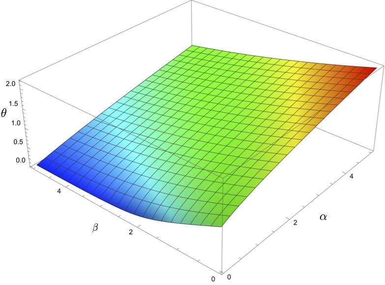
Figure 1. Simulation of $\theta(\alpha,\beta)$ for $(\alpha,\beta)\in(0,5)^{2}$

2. Computation of the Mellin transform of $X_{T}$

We start by proving Proposition 1. Recall that under $\mathbb{P}_{(x,y)}$ the pair $(X,Y)$ is a solution of the SDE, see [16, Chapter XI] :

$$X_{t}=x+2\int_{0}^{t}\sqrt{X_{s}}dB_{s}+\alpha t\qquad\text{and }\qquad Y_{t}=y+2\int_{0}^{t}\sqrt{Y_{s}}dW_{s}+\beta t,\quad\qquad t\geq 0,$$ (2.1)

where $B$ and $W$ are two independent Brownian motions. In the following, to simplify the notation, we shall write for a random variable $Z$ and for $\gamma\in\mathbb{R}$ :

$$\mathbb{E}[Z_{+}^{\gamma}]=\mathbb{E}[Z^{\gamma}1_{\{Z>0\}}].$$

Take $r,\nu\in(0,1)$ such that $r+\nu>1$ and $\nu<\frac{\alpha+\beta}{2}$. Applying the Markov property and the scaling property of squared Bessel processes, we have

$$\int_{0}^{+\infty}t^{-r}\mathbb{E}_{(0,y)}\left[(X_{t}-Y_{t})_{+}^{-\nu}\right]dt =\int_{0}^{+\infty}\mathbb{E}_{(0,y)}\left[(u+T)^{-r}\mathbb{E}_{(X_{T},X_{T})}\left[\left(X_{u}-Y_{u}\right)_{+}^{-\nu}\right]1_{\{T<+\infty\}}\right]du$$

$$=\int_{0}^{+\infty}\mathbb{E}_{(0,y)}\left[X_{T}^{1-\nu}(sX_{T}+T)^{-r}1_{\{T<+\infty\}}\right]\mathbb{E}_{(1,1)}\left[\left(X_{s}-Y_{s}\right)_{+}^{-\nu}\right]ds.$$ (2.2)

Note that we cannot just take $r=0$, as both sides would be infinite. Indeed, in this case, for the left-hand side to be finite, the integral in $t$ requires that $\nu>1$ while the expectation requires that $\nu<1$. To compute the positive parts in (2.2), recall the formula for any positive r.v. $Z$ which admits some negative moments, see [14, Lemma 1] :

$$\mathbb{E}\left[Z_{+}^{-\nu}\right]=\frac{\Gamma(1-\nu)}{\pi}\int_{0}^{+\infty}\lambda^{\nu-1}\mathbb{E}\left[\sin\left(\lambda Z+\frac{\pi}{2}\nu\right)\right]d\lambda.$$

From [16, Chapter XI], the Fourier transform of $X-Y$ is given, since $X$ and $Y$ are independent, by

$$\mathbb{E}_{(x,y)}\left[e^{\textbf{i}\lambda(X_{t}-Y_{t})}\right]=(1-2\textbf{i}\lambda t)^{-\alpha/2}(1+2\textbf{i}\lambda t)^{-\beta/2}\exp\left(\frac{\textbf{i}\lambda(x-y)-2\lambda^{2}t(x+y)}{1+4\lambda^{2}t^{2}}\right)$$

hence, after a change of variable

$$\frac{\pi}{\Gamma(1-\nu)}\mathbb{E}_{(x,y)}\left[\left(X_{t}-Y_{t}\right)_{+}^{-\nu}\right]\\ =t^{-\nu}\Im\left(e^{\textbf{i}\frac{\pi}{2}\nu}\int_{0}^{+\infty}\xi^{\nu-1}(1-2\textbf{i}\xi)^{-\alpha/2}(1+2\textbf{i}\xi)^{-\beta/2}\exp\left(\frac{\textbf{i}\xi(x-y)-2\xi^{2}(x+y)}{t(1+4\xi^{2})}\right)d\xi\right)$$$$ (2.3)

where $\Im$ denotes the imaginary part. On the one hand, taking $x=0$ in (2.3) and plugging this expression in (2.2), we deduce thank to Fubini’s theorem that the left-hand side of (2.2) equals

$$\frac{\Gamma(1-\nu)\Gamma(r+\nu-1)}{\pi y^{r+\nu-1}}\Im\left(e^{\textbf{i}\frac{\pi}{2}(1-r)}\int_{0}^{+\infty}\xi^{-r}(1-2\textbf{i}\xi)^{-\frac{\alpha}{2}}(1+2\textbf{i}\xi)^{r+\nu-1-\frac{\beta}{2}}\right)d\xi.$$

Similarly, plugging (2.3) with $x=y=1$ in the right-hand side of (2.2) and applying Fubini’s theorem, we obtain

$$\frac{\Gamma(1-\nu)\Gamma(r+\nu-1)}{\pi}\Im\left(e^{\textbf{i}\frac{\pi}{2}\nu}\int_{0}^{+\infty}\xi^{\nu-1}(1-2\textbf{i}\xi)^{-\alpha/2}(1+2\textbf{i}\xi)^{-\beta/2}G_{r,\nu}(\xi)d\xi\right)$$

where, using a change of variables and an integration by parts,

$$G_{r,\nu}(\xi) =\frac{1}{\Gamma(r+\nu-1)}\mathbb{E}_{(0,y)}\left[X_{T}^{1-\nu}\int_{0}^{+\infty}(uX_{T}+T)^{-r}u^{-\nu}e^{-\frac{4\xi^{2}}{u(1+4\xi^{2})}}du1_{\{T<+\infty\}}\right]$$

$$=\frac{1}{\Gamma(\nu+r)}\mathbb{E}_{(0,y)}\left[X_{T}^{1-\nu}\int_{0}^{+\infty}s^{\nu+r-1}(X_{T}+Ts)^{-r}e^{-\eta(\xi)s}\left(r\frac{T}{X_{T}+Ts}+\eta(\xi)\right)ds1_{\{T<+\infty\}}\right]$$

and where we have set, to simplify the notation, $\displaystyle\eta(\xi)=\frac{4\xi^{2}}{1+4\xi^{2}}$. As a consequence, Equation (2.2) now reads

$$\frac{1}{y^{r+\nu-1}}\Im\left(e^{\textbf{i}\frac{\pi}{2}(1-r)}\int_{0}^{+\infty}\xi^{-r}(1-2\textbf{i}\xi)^{-\frac{\alpha}{2}}(1+2\textbf{i}\xi)^{r+\nu-1-\frac{\beta}{2}}d\xi\right)\\ =\Im\left(e^{\textbf{i}\frac{\pi}{2}\nu}\int_{0}^{+\infty}\xi^{\nu-1}(1-2\textbf{i}\xi)^{-\frac{\alpha}{2}}(1+2\textbf{i}\xi)^{-\frac{\beta}{2}}G_{r,\nu}(\xi)d\xi\right)$$ (2.4)

and this formula extends by analyticity to $r+\nu>0$. By monotone convergence, we then deduce that

$$G_{r,\nu}(\xi)\xrightarrow[r\downarrow 0]{}\frac{1}{\Gamma(\nu)}\mathbb{E}_{(0,y)}\left[X_{T}^{1-\nu}\int_{0}^{+\infty}s^{\nu-1}e^{-\eta(\xi)s}\eta(\xi)ds1_{\{T<+\infty\}}\right]=\mathbb{E}_{(0,y)}\left[X_{T}^{1-\nu}1_{\{T<+\infty\}}\right]\left(\eta(\xi)\right)^{1-\nu}.$$

As a consequence, letting $r\downarrow 0$ in (2.4), we obtain the formula

$$\frac{1}{y^{\nu-1}}\Im\left(\textbf{i}\int_{0}^{+\infty}(1-2\textbf{i}\xi)^{-\frac{\alpha}{2}}(1+2\textbf{i}\xi)^{\nu-1-\frac{\beta}{2}}d\xi\right)\\ =\mathbb{E}_{(0,y)}\left[X_{T}^{1-\nu}1_{\{T<+\infty\}}\right]\Im\left(e^{\textbf{i}\frac{\pi}{2}\nu}\int_{0}^{+\infty}\xi^{1-\nu}(1-2\textbf{i}\xi)^{\nu-1-\alpha/2}(1+2\textbf{i}\xi)^{\nu-1-\beta/2}d\xi\right)$$ (2.5)

and it remains to compute both integrals. Let us start with the left-hand side. Taking the imaginary part in Lemma 9 from the Appendix, we have

$$\Im\left(\textbf{i}\int_{0}^{+\infty}\xi^{\gamma-1}(1-2\textbf{i}\xi)^{-\lambda}(1+2\textbf{i}\xi)^{-\mu}d\xi\right)\\ =\frac{\Gamma(\gamma)\Gamma(\mu+\lambda-\gamma)}{\Gamma(\lambda)\Gamma(\mu)}2^{-\gamma}\left(\cos\left(\frac{\pi}{2}\gamma\right)B\left(\lambda,1-\gamma\right)2^{-\lambda}{}_{2}F_{1}\biggl{[}\genfrac{.}{.}{0.0pt}{}{1-\mu\quad\lambda}{\lambda-\gamma+1};\frac{1}{2}\biggr{]}\right.\\ \left.+\cos\left(\frac{\pi}{2}\gamma\right)B\left(\mu,1-\gamma\right)2^{-\mu}{}_{2}F_{1}\biggl{[}\genfrac{.}{.}{0.0pt}{}{1-\lambda\quad\mu}{\mu-\gamma+1};\frac{1}{2}\biggr{]}\right).$$

Letting $\gamma\uparrow 1$ and using the formula $\displaystyle{}_{2}F_{1}\biggl{[}\genfrac{.}{.}{0.0pt}{}{a\quad b}{b};\frac{1}{2}\biggr{]}=2^{-a}$, we thus deduce that

$$\Im\left(\textbf{i}\int_{0}^{+\infty}(1-2\textbf{i}\xi)^{-\frac{\alpha}{2}}(1+2\textbf{i}\xi)^{\nu-1-\frac{\beta}{2}}d\xi\right)=\frac{\pi\Gamma\left(\frac{\alpha+\beta}{2}-\nu\right)}{\Gamma(\frac{\alpha}{2})\Gamma(\frac{\beta}{2}+1-\nu)}2^{\nu-\frac{\alpha+\beta}{2}-1}.$$ (2.6)

On the other side, multiplying Lemma 9 in the Appendix by $e^{\textbf{i}\frac{\pi}{2}\nu}$ and taking the imaginary part, we observe that only the first term will remain, i.e.

$$\Im\left(e^{\textbf{i}\frac{\pi}{2}\nu}\int_{0}^{+\infty}\xi^{1-\nu}(1-2\textbf{i}\xi)^{\nu-1-\alpha/2}(1+2\textbf{i}\xi)^{\nu-1-\beta/2}d\xi\right)\\ =-\frac{\Gamma(2-\nu)\Gamma\left(\frac{\alpha+\beta}{2}-\nu\right)}{\Gamma\left(\frac{\beta}{2}+1-\nu\right)}2^{\nu-2}\sin(\pi\nu)\frac{\Gamma(\nu-1)}{\Gamma\left(\frac{\alpha}{2}\right)}2^{\nu-1-\frac{\alpha}{2}}{}_{2}F_{1}\biggl{[}\genfrac{.}{.}{0.0pt}{}{\nu-\frac{\beta}{2}\quad\frac{\alpha}{2}+1-\nu}{\frac{\alpha}{2}};\frac{1}{2}\biggr{]}.$$ (2.7)

Plugging (2.6) and (2.7) in (2.5) and using the reflection formula for the Gamma function, i.e. $\Gamma(2-\nu)\sin(\pi\nu)\Gamma(\nu-1)=-\pi$ for $\nu\in(0,1)$, we finally conclude that

$$\mathbb{E}_{(0,y)}\left[X_{T}^{1-\nu}1_{\{T<+\infty\}}\right]=\left(2y\right)^{1-\nu}\frac{2^{1-\frac{\beta}{2}}}{{}_{2}F_{1}\biggl{[}\genfrac{.}{.}{0.0pt}{}{\nu-\frac{\beta}{2}\quad\frac{\alpha}{2}+1-\nu}{\frac{\alpha}{2}};\frac{1}{2}\biggr{]}}$$ (2.8)

and the result follows from Euler’s transformation

$${}_{2}F_{1}\biggl{[}\genfrac{.}{.}{0.0pt}{}{\nu-\frac{\beta}{2}\quad\frac{\alpha}{2}+1-\nu}{\frac{\alpha}{2}};\frac{1}{2}\biggr{]}=2^{1-\frac{\beta}{2}}{}_{2}F_{1}\biggl{[}\genfrac{.}{.}{0.0pt}{}{\frac{\alpha+\beta}{2}-\nu\quad\nu-1}{\frac{\alpha}{2}};\frac{1}{2}\biggr{]}=2^{1-\frac{\beta}{2}}F_{\alpha,\beta}(1-\nu).$$

In particular, letting $\nu\uparrow 1$ in (2.8), we deduce that $\mathbb{P}(T<+\infty)=1$ which implies that $T$ is a.s. finite. $\square$

3. Some first estimates

3.1. From $\mathbb{P}_{(x,y)}$ to $\mathbb{P}_{(0,1)}$

Before tackling the proof of Theorem 2, we gather here some preliminary computations. We start by proving that the finiteness of $\mathbb{E}_{(x,y)}[T^{\lambda}]$ is equivalent to that of $\mathbb{E}_{(0,1)}[T^{\lambda}]$.

Lemma 5.

Let $0\leq x<y$ be fixed. There exists two positive constants $\kappa_{1},\kappa_{2}$ such that for $0\leq\lambda\leq\theta$,

$$\kappa_{1}\mathbb{E}_{(0,1)}\left[T^{\lambda}\right]-\kappa_{2}\leq\mathbb{E}_{(x,y)}\left[T^{\lambda}\right]\leq y^{\lambda}\mathbb{E}_{(0,1)}\left[T^{\lambda}\right].$$

Proof.

Notice first that by a coupling argument $\mathbb{P}_{(x,y)}(T\geq t)\leq\mathbb{P}_{(0,y)}\left(T\geq t\right)$ which implies by scaling that for $\lambda\geq 0$ :

$$\mathbb{E}_{(x,y)}\left[T^{\lambda}\right]\leq\mathbb{E}_{(0,y)}\left[T^{\lambda}\right]=y^{\lambda}\mathbb{E}_{(0,1)}\left[T^{\lambda}\right].$$

To prove a converse inequality, take $a\in(0,y)$ and let us denote by $\tau_{y}=\inf\{t\geq 0,\;Y_{t}=y\}$ the first hitting time of $y$ by the process $Y$. Then, applying the strong Markov property at the time $\tau_{y}$,

$$\mathbb{P}_{(0,a)}(T>t) =\mathbb{P}_{(0,a)}(T>t,T\leq\tau_{y})+\mathbb{P}_{(0,a)}(T>t,T>\tau_{y})$$

$$\leq 2\mathbb{P}_{(0,a)}(\tau_{y}>t)+\mathbb{E}_{(0,a)}\left[\mathbb{P}_{(X_{\tau_{y}},y)}(T>t-s)_{|s=\tau_{y}}1_{\{T>\tau_{y}\}}1_{\{\tau_{y}\leq t\}}\right]$$

hence, for $\lambda\leq\theta$, using the standard inequality $(a+b)^{\lambda}\leq 2^{\lambda}(a^{\lambda}+b^{\lambda})$,

$$\mathbb{E}_{(0,a)}[T^{\lambda}] \leq 2\mathbb{E}_{(0,a)}[\tau_{y}^{\lambda}]+\int_{0}^{y}\int_{0}^{+\infty}\mathbb{E}_{(z,y)}[(T+s)^{\lambda}]\mathbb{P}_{(0,a)}(X_{\tau_{y}}\in dz,\tau_{y}\in ds)$$

$$\leq 2\mathbb{E}_{(0,a)}[\tau_{y}^{\lambda}]+2^{\lambda}\int_{0}^{y}\int_{0}^{+\infty}\left(\mathbb{E}_{(z,y)}[T^{\lambda}]+s^{\lambda}\right)\mathbb{P}_{(0,a)}(X_{\tau_{y}}\in dz,\tau_{y}\in ds)$$

$$\leq(2+2^{\theta})\mathbb{E}_{(0,a)}[\tau_{y}^{\lambda}]+2^{\theta}\int_{0}^{y}\mathbb{E}_{(z,y)}[T^{\lambda}]\mathbb{P}_{(0,a)}(X_{\tau_{y}}\in dz).$$ (3.1)

Recall then that, since $Y_{0}=a<y$, the r.v. $\tau_{y}$ admits positive moments of all orders, see for instance [18], so the first term on the right-hand side is always finite. Now let $\delta\in(0,y)$. Since the function $z\rightarrow\mathbb{E}_{(z,y)}[T^{\lambda}]$ is decreasing on $[0,y]$, we have

$$\int_{0}^{y}\mathbb{E}_{(z,y)}[T^{\lambda}]\mathbb{P}_{(0,a)}(X_{\tau_{y}}\in dz)\leq\mathbb{E}_{(0,y)}[T^{\lambda}]\mathbb{P}_{(0,a)}(X_{\tau_{y}}\leq\delta)+\mathbb{E}_{(\delta,y)}[T^{\lambda}].$$

As a consequence, plugging this last inequality in (3.1) and using the scaling property, we obtain the bound

$$\left(a^{\lambda}-2^{\theta}y^{\lambda}\mathbb{P}_{(0,a)}(X_{\tau_{y}}\leq\delta)\right)\mathbb{E}_{(0,1)}[T^{\lambda}]\leq(2+2^{\theta})\mathbb{E}_{(0,a)}[\tau_{y}^{\lambda}]+2^{\theta}\mathbb{E}_{(\delta,y)}[T^{\lambda}]$$ (3.2)

in which we shall take $\delta$ small enough for the left-hand side to be strictly positive. Finally, it remains to write, applying the Markov property,

$$\mathbb{E}_{(x,y)}[(1+T)^{\lambda}]\geq\mathbb{E}\left[1_{\{T>1,Y_{1}>y,X_{1}\leq\delta\}}\mathbb{E}_{(X_{1},Y_{1})}[T^{\lambda}]\right]\geq\mathbb{E}\left[1_{\{T>1,Y_{1}>y,X_{1}\leq\delta\}}\right]\mathbb{E}_{(\delta,y)}[T^{\lambda}]$$

hence, going back to (3.2), we have thus proven that for $0\leq\lambda\leq\theta$,

$$c_{1}\mathbb{E}_{(0,1)}\left[T^{\lambda}\right]\leq c_{2}+\mathbb{E}_{(x,y)}[(1+T)^{\lambda}]\leq c_{2}+2^{\theta}+2^{\theta}\mathbb{E}_{(x,y)}[T^{\lambda}]$$

where $c_{1},c_{2}$ are two positive constants. This is the lower bound of Lemma 5 after renaming the constants. $\square$

3.2. Maximal inequalities

To go from $X_{T}$ to $T$, we shall rely on maximal inequalities for squared Bessel processes. Indeed, recall from [6] that there exist two constants $c_{\alpha,\lambda}$ and $C_{\alpha,\lambda}$ such that for any stopping time $\zeta$ (with respect to $X$) :

$$c_{\alpha,\lambda}\mathbb{E}_{(0,1)}[\zeta^{\lambda}]\leq\mathbb{E}_{(0,1)}\left[\sup_{s\leq\zeta}X_{s}^{\lambda}\right]\leq C_{\alpha,\lambda}\mathbb{E}_{(0,1)}[\zeta^{\lambda}].$$ (3.3)

As a consequence, taking $\zeta=T$, we first deduce that

$$\mathbb{E}_{(0,1)}\left[X_{T}^{\lambda}\right]\leq\mathbb{E}_{(0,1)}\left[\sup_{s\leq T}X_{s}^{\lambda}\right]\leq C_{\alpha,\lambda}\mathbb{E}_{(0,1)}[T^{\lambda}]$$ (3.4)

which implies that $\mathbb{E}_{(0,1)}\left[T^{\lambda}\right]=+\infty$ as soon as $\lambda\geq\theta$. Note that a converse inequality exists : from Pedersen [13], if $\lambda>1-\alpha/2$ and $\zeta$ is a stopping time such that $\mathbb{E}_{(0,1)}[\zeta^{\lambda}]<+\infty$, then

$$\mathbb{E}_{(0,1)}\left[\sup_{s\leq\zeta}X_{s}^{\lambda}\right]\leq\left(\frac{2\lambda}{2\lambda-(2-\alpha)}\right)^{\frac{2\lambda}{2-\alpha}}\mathbb{E}_{(0,1)}\left[X_{\zeta}^{\lambda}\right].$$ (3.5)

Unfortunately, to apply this inequality in our set-up, one needs the assumption that $T$ admits moments of order up to $\theta$, which is precisely what we wish to prove.

4. Proof of Theorem 2

We prove in this section that $\mathbb{E}_{(0,1)}[T^{\lambda}]$ is finite for $0\leq\lambda<\theta$. To do so, we shall separate the two cases $\alpha\leq\beta$ and $\alpha>\beta$.

4.1. The case $\alpha\leq\beta$

Recall that in this case $\theta\in(0,1]$. We first show that $\theta>1-\frac{\beta}{2}$. Indeed, since the paths of $X$ and $Y$ are continuous and non-negative, the path inequality $T\leq\tau_{0}$ implies that $\mathbb{E}_{(0,1)}[T^{\lambda}]\leq\mathbb{E}_{(0,1)}[\tau_{0}^{\lambda}]$. The right-hand side is finite if and only if $\beta<2$ and $\lambda<1-\frac{\beta}{2}$, see for instance [9]. As a consequence, we deduce the lower bound $\theta>1-\frac{\beta}{2}$, with a strict inequality since $F_{\alpha,\beta}\left(1-\frac{\beta}{2}\right)=2^{\frac{\beta}{2}-1}>0$.

We shall now construct a martingale. Let us set for $z>0$

$$\Psi^{(\beta)}_{\lambda}(z):=z^{\frac{\eta}{2}}K_{\eta}\left(\sqrt{2\lambda z}\right)=2^{\frac{\eta}{2}-1}\lambda^{\frac{\eta}{2}}\int_{0}^{+\infty}e^{-\lambda s}e^{-\frac{z}{2s}}s^{\eta-1}ds$$ (4.1)

where $\eta=1-\frac{\beta}{2}\in(-\infty,1)$ and $K_{\eta}$ denotes the usual McDonald’s function. In particular, $\Psi^{(\beta)}_{\lambda}$ is a solution of the ordinary differential equation :

$$zf^{\prime\prime}(z)+\frac{\beta}{2}f^{\prime}(z)-\frac{\lambda}{2}f(z)=0$$ (4.2)

such that $\displaystyle\lim_{z\rightarrow+\infty}\Psi^{(\beta)}_{\lambda}(z)=0$. Take $Y_{0}=y>0$ and $0<\varepsilon<y$. Applying Itô’s formula, we deduce from (4.2) that the process

$$M_{t}=e^{-\lambda t}\Psi_{\lambda}^{(\beta)}\left(Y_{T\wedge\tau_{\varepsilon}}\right),\quad t<\tau_{\varepsilon}$$

is a bounded local martingale, hence a true martingale under $\mathbb{P}_{(0,y)}$. Then Doob’s optional sampling theorem yields the identity

$$\mathbb{E}_{(0,y)}\left[e^{-\lambda T\wedge\tau_{\varepsilon}}\Psi_{\lambda}^{(\beta)}\left(Y_{T\wedge\tau_{\varepsilon}}\right)\right]=\Psi_{\lambda}^{(\beta)}(y).$$

Inverting these Laplace transforms thanks to (4.1), we deduce that

$$\int_{0}^{t}s^{\eta-1}\mathbb{E}_{(0,y)}\left[1_{\{T\wedge\tau_{\varepsilon}>t-s\}}e^{-\frac{Y_{T\wedge\tau_{\varepsilon}}}{2s}}\right]ds=\int_{t}^{+\infty}s^{\eta-1}\mathbb{E}_{(0,y)}\left[e^{-\frac{y}{2s}}-e^{-\frac{Y_{T\wedge\tau_{\varepsilon}}}{2s}}\right]ds=:H_{\varepsilon}(t).$$ (4.3)

In particular, applying the Fubini theorem, the Mellin transform of $H_{\varepsilon}$ is given for $\lambda>\eta$ by :

$$\int_{0}^{+\infty}t^{\lambda-\eta-1}H_{\varepsilon}(t)dt=\int_{0}^{+\infty}s^{\lambda-1}\mathbb{E}_{(0,y)}\left[e^{-\frac{y}{2s}}-e^{-\frac{Y_{T\wedge\tau_{\varepsilon}}}{2s}}\right]ds=\frac{2^{-\lambda}}{\lambda-\eta}\Gamma(-\lambda)\left(y^{\lambda}-\mathbb{E}_{(0,y)}\left[Y_{T\wedge\tau_{\varepsilon}}^{\lambda}\right]\right)$$ (4.4)

Note that the condition $\lambda>\eta$ is not restrictive, as we know that $\theta>\eta$. We now come back to (4.3) and observe that :

$$H_{\varepsilon}(t) \geq\mathbb{E}_{(0,y)}\left[1_{\{T>t\}}\int_{0}^{t}s^{\eta-1}e^{-\frac{Y_{T\wedge\tau_{\varepsilon}}}{2s}}ds\,1_{\{Y_{T\wedge\tau_{\varepsilon}}\leq t\}}\right]$$

$$\geq\mathbb{P}_{(0,y)}\left(T\wedge\tau_{\varepsilon}>t,Y_{T\wedge\tau_{\varepsilon}}\leq t\right)\int_{0}^{t}s^{\eta-1}e^{-\frac{t}{2s}}ds$$

$$\geq t^{\eta}\left(\mathbb{P}_{(0,y)}\left(T\wedge\tau_{\varepsilon}>t\right)-\mathbb{P}_{(0,y)}\left(Y_{T\wedge\tau_{\varepsilon}}>t\right)\right)\int_{0}^{1}s^{\eta-1}e^{-\frac{1}{2s}}ds.$$

Integrating this relation against $(\lambda-\eta)t^{\lambda-\eta-1}$ on $(0,+\infty)$ for $\lambda\in(\eta,1)$, we deduce from (4.4) that there exists a constant $K$ such that

$$\mathbb{E}_{(0,y)}\left[\left(T\wedge\tau_{\varepsilon}\right)^{\lambda}\right] \leq\mathbb{E}_{(0,y)}\left[Y_{T\wedge\tau_{\varepsilon}}^{\lambda}\right]\left(1-\frac{2^{-\lambda}K}{\lambda-\eta}\Gamma(-\lambda)\right)+\frac{2^{-\lambda}K}{\lambda-\eta}\Gamma(-\lambda)y^{\lambda}$$

$$\leq\left(\mathbb{E}_{(0,y)}\left[Y_{T}^{\lambda}\right]+\varepsilon^{\lambda}\right)\left(1-\frac{2^{-\lambda}K}{\lambda-\eta}\Gamma(-\lambda)\right)+\frac{2^{-\lambda}K}{\lambda-\eta}\Gamma(-\lambda)y^{\lambda}$$

The upper bound of Theorem 2 now follows by letting $\varepsilon\downarrow 0$ and applying the monotone convergence theorem. $\square$

Remark 6.

Note that this argument no longer holds for $\alpha>\beta$. Indeed, in this latter case $\theta>1$, but since the right-hand side has a pole at $\lambda=1$ (coming from the Mellin transform of $H_{\varepsilon}$), we can only deduce that $\mathbb{E}_{(0,1)}[T^{\lambda}]<+\infty$ for $\lambda\in(0,1)$.

4.2. The case $\alpha>\beta$

Let us define

$$\gamma=\sup\{s\geq 0,\;\mathbb{E}_{(0,y)}[T^{s}]<+\infty\}.$$

We already know from (3.4) that $\gamma\leq\theta$ so let us assume that $\gamma<\theta$. We shall prove by contradiction that this is not possible.

4.2.1. First step

We first prove that if $\gamma<\theta$, then $\mathbb{E}_{(0,y)}[T^{\gamma}]<+\infty$, i.e. that the supremum in the definition of $\gamma$ is attained. To do so, observe first that as explained in Remark 6, $\gamma\geq 1$. This may also be checked using the following argument : since $\alpha>\beta$, the SDE (2.1) defining $X$ and $Y$ implies that the process

$$M_{t\wedge T}=Y_{t\wedge T}-X_{t\wedge T}+(\alpha-\beta)t\wedge T=y+\int_{0}^{t\wedge T}\sqrt{Y_{s}}dW_{s}-\int_{0}^{t\wedge T}\sqrt{X_{s}}dB_{s},\qquad t\geq 0$$

is a positive local martingale, hence a supermartingale. Applying Fatou’s lemma, we thus have

$$(\alpha-\beta)\mathbb{E}[T]=\mathbb{E}\left[\liminf_{t\rightarrow+\infty}M_{t\wedge T}\right]\leq\liminf_{t\rightarrow+\infty}\mathbb{E}\left[M_{t\wedge T}\right]\leq\mathbb{E}\left[M_{0}\right]=y$$

which proves that $T$ is integrable, i.e. $\gamma\geq 1$. In particular, $\gamma>1-\alpha/2$, which allows us to apply the maximal inequality of Pedersen [13] recalled in (3.5). Take $\varepsilon>0$. By definition of $\gamma$, $\mathbb{E}_{(0,y)}[T^{\gamma-\varepsilon}]<+\infty$, hence we have :

$$\mathbb{E}_{(0,y)}\left[\sup_{s\leq T}X_{s}^{\gamma-\varepsilon}\right]\leq\left(\frac{2(\gamma-\varepsilon)}{2(\gamma-\varepsilon)-(2-\alpha)}\right)^{\frac{2(\gamma-\varepsilon)}{2-\alpha}}\mathbb{E}_{(0,y)}\left[X_{T}^{\gamma-\varepsilon}\right].$$

Using (3.3), we thus deduce from Fatou’s lemma and the monotone convergence theorem that

$$c_{\alpha,r}\mathbb{E}_{(0,y)}[T^{\gamma}]\leq c_{\alpha,r}\liminf_{\varepsilon\rightarrow 0}\mathbb{E}_{(0,y)}[T^{\gamma-\varepsilon}]\leq\left(\frac{2\gamma}{2\gamma-(2-\alpha)}\right)^{\frac{2\gamma}{2-\alpha}}\left(1+\mathbb{E}_{(0,y)}\left[X_{T}^{\gamma}1_{\{X_{T}\geq 1\}}\right]\right)<+\infty$$

since $\gamma<\theta$. As a consequence, the supremum in the definition of $\gamma$ is attained.

4.2.2. Second step

We shall now contradict the definition of $\gamma$ by showing that $T$ admits moments of order $\gamma+\varepsilon$ for some $\varepsilon>0$ small enough. To do so, notice first, still from the SDE (2.1), that since $\alpha>\beta$, the process $(\alpha Y_{t\wedge T}-\beta X_{t\wedge T},\;t\geq 0)$ is a positive local martingale under $\mathbb{P}_{(0,y)}$. Let us set

$$A_{t}=\int_{0}^{t}(\beta^{2}X_{s}+\alpha^{2}Y_{s})ds,\qquad t\geq 0,$$

and observe that for $z>0$, the bounded process

$$\exp\left(z(\beta X_{t\wedge T}-\alpha Y_{t\wedge T})-\frac{z^{2}}{2}A_{t\wedge T}\right),\qquad t\geq 0,$$ (4.5)

is a positive martingale under $\mathbb{P}_{(0,y)}$. Applying Doob’s optional stopping theorem and the dominated convergence theorem, we deduce that

$$\mathbb{E}_{(0,y)}\left[e^{-z(\alpha-\beta)X_{T}-\frac{z^{2}}{2}A_{T}}\right]=e^{-z\alpha y}.$$ (4.6)

The next lemma shows that the finiteness of the moments of $T$ is equivalent to those of $\sqrt{A_{T}}$.

Lemma 7.

For $\lambda\in[0,\theta)$,

$$\mathbb{E}_{(0,y)}[T^{\lambda}]<+\infty\qquad\Longleftrightarrow\qquad\mathbb{E}_{(0,y)}\left[A_{T}^{\frac{\lambda}{2}}\right]<+\infty.$$

Proof.

On the one hand, applying Cauchy-Schwarz’s inequality and Formula (3.3),

$$\mathbb{E}_{(0,y)}\left[A_{T}^{\frac{\lambda}{2}}\right] \leq\mathbb{E}_{(0,y)}\left[T^{\frac{\lambda}{2}}\left(2\alpha^{2}\sup_{s\leq T}Y_{s}\right)^{\frac{\lambda}{2}}\right]$$

$$\leq\mathbb{E}_{(0,y)}\left[T^{\lambda}\right]^{\frac{1}{2}}(\sqrt{2}\alpha)^{\lambda}\mathbb{E}_{(0,y)}\left[\sup_{s\leq T}Y_{s}^{\lambda}\right]^{\frac{1}{2}}\leq(\sqrt{2}\alpha)^{\lambda}\sqrt{C_{\alpha,r}}\mathbb{E}_{(0,y)}\left[T^{\lambda}\right]$$

which proves the implication. On the other hand, going back to the SDE (2.1) defining $X$ and applying the Burkholder-Davis-Gundy inequality, we deduce that there exists a constant $K_{\lambda}$ such that

$$\alpha^{\lambda}\mathbb{E}_{(0,y)}[T^{\lambda}] \leq\mathbb{E}_{(0,y)}\left[\left(y+X_{T}+\left|\int_{0}^{T}\sqrt{X_{s}}dB_{s}\right|\right)^{\lambda}\right]$$

$$\leq K_{\lambda}\left(y^{\lambda}+\mathbb{E}_{(0,y)}[X_{T}^{\lambda}]+\mathbb{E}_{(0,y)}\left[\left|\int_{0}^{T}X_{s}ds\right|^{\frac{\lambda}{2}}\right]\right)$$

$$\leq K_{\lambda}\left(y^{\lambda}+\mathbb{E}_{(0,y)}[X_{T}^{\lambda}]+\frac{1}{\alpha^{\lambda}}\mathbb{E}_{(0,y)}\left[A_{T}^{\frac{\lambda}{2}}\right]\right)$$

which concludes the proof of Lemma 7 since $X_{T}$ admits moments of order $\lambda<\theta$. $\square$

Thanks to Lemma 7, it is thus enough to prove that $\mathbb{E}_{(0,y)}\left[A_{T}^{\frac{\gamma+\varepsilon}{2}}\right]<+\infty$ for some $\varepsilon>0$ small enough such that $\gamma+\varepsilon<\theta$. We now set $n$ equal to the integer part of $\gamma$ : $n=\lfloor\gamma\rfloor$. Differentiating $n+1$ times Formula (4.6) with respect to $z$ and applying Leibniz rule, we obtain

$$\sum_{k=0}^{n+1}\binom{n+1}{k}(\alpha-\beta)^{k}\mathbb{E}_{(0,y)}\left[X_{T}^{k}A_{T}^{\frac{n+1-k}{2}}H_{n+1-k}(z\sqrt{A_{T}})e^{-z(\alpha-\beta)X_{T}-\frac{z^{2}}{2}A_{T}}\right]=(\alpha y)^{n+1}e^{-z\alpha y}$$ (4.7)

where the sequence $(H_{k})_{k\geq 0}$ denotes the Hermite’s polynomials. In particular, for any $k\in\mathbb{N}$, since $H_{k}$ is a polynomial, there exists a finite constant $c_{k}$ such that

$$\sup_{x\geq 0}|H_{k}(x)|e^{-\frac{1}{4}x^{2}}<c_{k}.$$

Take $\varepsilon$ small enough such that $n+1-\gamma-\varepsilon>0$ and $\gamma+\varepsilon<\theta$. We now integrate (4.7) against $z^{n-\gamma-\varepsilon}$ on $(0,+\infty)$, applying repeatedly the Fubini-Tonelli theorem.

1. The right-hand side gives :

   $$(\alpha y)^{n+1}\int_{0}^{+\infty}z^{n-\gamma-\varepsilon}e^{-z\alpha y}dz=\Gamma(n+1-\gamma-\varepsilon)(\alpha y)^{\gamma+\varepsilon}$$

2. The term for $k=n+1$ gives :

   $$(\alpha-\beta)^{n+1}\int_{0}^{+\infty}z^{n-\gamma-\varepsilon}\mathbb{E}_{(0,y)}\left[X_{T}^{n+1}e^{-z(\alpha-\beta)X_{T}-\frac{z^{2}}{2}A_{T}}\right]dz\\ \leq\Gamma(n+1-\gamma-\varepsilon)(\alpha-\beta)^{\gamma+\varepsilon}\mathbb{E}_{(0,y)}\left[X_{T}^{\gamma+\varepsilon}\right]<+\infty.$$

3. The main sum, for $1\leq k\leq n$ gives :

   $$\left|\sum_{k=1}^{n}\binom{n+1}{k}(\alpha-\beta)^{k}\int_{0}^{+\infty}z^{n-\gamma-\varepsilon}\mathbb{E}_{(0,y)}\left[X_{T}^{k}A_{T}^{\frac{n+1-k}{2}}H_{n+1-k}(z\sqrt{A_{T}})e^{-z(\alpha-\beta)X_{T}-\frac{z^{2}}{2}A_{T}}\right]dz\right|$$

   $$\qquad\leq\sum_{k=1}^{n}\binom{n+1}{k}(\alpha-\beta)^{k}c_{n+1-k}\int_{0}^{+\infty}z^{n-\gamma-\varepsilon}\mathbb{E}_{(0,y)}\left[X_{T}^{k}A_{T}^{\frac{n+1-k}{2}}e^{-\frac{z^{2}}{4}A_{T}}\right]dz$$

   $$\qquad=\Gamma\left(\frac{n+1-\gamma-\varepsilon}{2}\right)2^{n-\gamma-\varepsilon}\sum_{k=1}^{n}\binom{n+1}{k}(\alpha-\beta)^{k}c_{n+1-k}\mathbb{E}_{(0,y)}\left[X_{T}^{k}A_{T}^{\frac{\gamma+\varepsilon-k}{2}}\right].$$

   Furthermore, applying Hölder’s inequality, the expectation in the sum on the right-hand side is smaller than

   $$\mathbb{E}_{(0,y)}\left[X_{T}^{k}A_{T}^{\frac{\gamma+\varepsilon-k}{2}}\right]\leq\mathbb{E}_{(0,y)}\left[X_{T}^{\frac{\gamma}{k-\varepsilon}}\right]^{\frac{k-\varepsilon}{\gamma}}\mathbb{E}_{(0,y)}\left[A_{T}^{\frac{\gamma}{2}}\right]^{\frac{\gamma+\varepsilon-k}{\gamma}}<+\infty$$ (4.8)

   which is finite provided that $\varepsilon$ is small enough so that $\gamma<\theta(1-\varepsilon)$.

4. As for the last term $k=0$, let us take $\delta>0$ and first write :

   $$\left|\int_{0}^{+\infty}z^{n-\gamma-\varepsilon}\mathbb{E}_{(0,y)}\left[A_{T}^{\frac{n+1}{2}}H_{n+1}(z\sqrt{A_{T}})e^{-z(\alpha-\beta)X_{T}-\frac{z^{2}}{2}A_{T}}1_{\{\delta\sqrt{A_{T}}\leq X_{T}\}}\right]dz\right|$$

   $$\qquad\leq c_{n+1}\int_{0}^{+\infty}z^{n-\gamma-\varepsilon}\mathbb{E}_{(0,y)}\left[A_{T}^{\frac{n+1}{2}}e^{-z(\alpha-\beta)X_{T}}1_{\{\delta\sqrt{A_{T}}\leq X_{T}\}}\right]dz$$

   $$\qquad=c_{n+1}\frac{\Gamma(n+1-\gamma-\varepsilon)}{(\alpha-\beta)^{n+1-\gamma-\varepsilon}}\mathbb{E}_{(0,y)}\left[A_{T}^{\frac{n+1}{2}}X_{T}^{-n-1+\gamma+\varepsilon}1_{\{\delta\sqrt{A_{T}}\leq X_{T}\}}\right]$$

   $$\qquad\leq c_{n+1}\frac{\Gamma(n+1-\gamma-\varepsilon)}{(\alpha-\beta)^{n+1-\gamma-\varepsilon}}\frac{1}{\delta^{n+1}}\mathbb{E}_{(0,y)}\left[X_{T}^{\gamma+\varepsilon}\right]<+\infty.$$

Plugging everything together, we have thus proven that for $\varepsilon>0$ small enough

$$\left|\int_{0}^{+\infty}z^{n-\gamma-\varepsilon}\mathbb{E}_{(0,y)}\left[A_{T}^{\frac{n+1}{2}}H_{n+1}(z\sqrt{A_{T}})e^{-z(\alpha-\beta)X_{T}-\frac{z^{2}}{2}A_{T}}1_{\{\delta\sqrt{A_{T}}>X_{T}\}}\right]dz\right|<+\infty.$$ (4.9)

We now study further this last expression, and assume, without loss of generality, that

$$\int_{0}^{+\infty}z^{n-\gamma-\varepsilon}H_{n+1}(z)e^{-\frac{z^{2}}{2}}dz>0.$$ (4.10)

Applying the Fubini-Tonelli theorem and a change of variables, we have :

$$\int_{0}^{+\infty}z^{n-\gamma-\varepsilon}\mathbb{E}_{(0,y)}\left[A_{T}^{\frac{n+1}{2}}H_{n+1}(z\sqrt{A_{T}})1_{\{H_{n+1}(z\sqrt{A_{T}})>0\}}e^{-z(\alpha-\beta)X_{T}-\frac{z^{2}}{2}A_{T}}1_{\{\delta\sqrt{A_{T}}>X_{T}\}}\right]dz$$

$$\qquad\qquad=\mathbb{E}_{(0,y)}\left[A_{T}^{\frac{\gamma+\varepsilon}{2}}1_{\{\delta\sqrt{A_{T}}>X_{T}\}}\int_{0}^{+\infty}z^{n-\gamma-\varepsilon}H_{n+1}(z)1_{\{H_{n+1}(z)>0\}}e^{-z(\alpha-\beta)\frac{X_{T}}{\sqrt{A_{T}}}-\frac{z^{2}}{2}}dz\right]$$

$$\qquad\qquad\geq\mathbb{E}_{(0,y)}\left[A_{T}^{\frac{\gamma+\varepsilon}{2}}1_{\{\delta\sqrt{A_{T}}>X_{T}\}}\right]\int_{0}^{+\infty}z^{n-\gamma-\varepsilon}H_{n+1}(z)1_{\{H_{n+1}(z)>0\}}e^{-z(\alpha-\beta)\delta-\frac{z^{2}}{2}}dz.$$

Similarly,

$$\int_{0}^{+\infty}z^{n-\gamma-\varepsilon}\mathbb{E}_{(0,y)}\left[A_{T}^{\frac{n+1}{2}}|H_{n+1}(z\sqrt{A_{T}})|1_{\{H_{n+1}(z\sqrt{A_{T}})<0\}}e^{-z(\alpha-\beta)X_{T}-\frac{z^{2}}{2}A_{T}}1_{\{\delta\sqrt{A_{T}}>X_{T}\}}\right]dz$$

$$\qquad\qquad\leq\mathbb{E}_{(0,y)}\left[A_{T}^{\frac{\gamma+\varepsilon}{2}}1_{\{\delta\sqrt{A_{T}}>X_{T}\}}\right]\int_{0}^{+\infty}z^{n-\gamma-\varepsilon}|H_{n+1}(z)|1_{\{H_{n+1}(z)<0\}}e^{-\frac{z^{2}}{2}}dz.$$

As a consequence, we deduce from (4.9) that

$$\mathbb{E}_{(0,y)}\left[A_{T}^{\frac{\gamma+\varepsilon}{2}}1_{\{\delta\sqrt{A_{T}}>X_{T}\}}\right]\int_{0}^{+\infty}z^{n-\gamma-\varepsilon}|H_{n+1}(z)|e^{-\frac{z^{2}}{2}}\left(1_{\{H_{n+1}(z)>0\}}e^{-z(\alpha-\beta)\delta}-1_{\{H_{n+1}(z)<0\}}\right)dz<+\infty.$$

But, from (4.10) the integral in $z$ is strictly positive for $\delta$ small enough. As a consequence, we have obtained that

$$\mathbb{E}_{(0,y)}\left[A_{T}^{\frac{\gamma+\varepsilon}{2}}1_{\{\delta\sqrt{A_{T}}>X_{T}\}}\right]<+\infty$$

and the result follows from the observation that

$$\mathbb{E}_{(0,y)}\left[A_{T}^{\frac{\gamma+\varepsilon}{2}}\right]\leq\mathbb{E}_{(0,y)}\left[A_{T}^{\frac{\gamma+\varepsilon}{2}}1_{\{\delta\sqrt{A_{T}}>X_{T}\}}\right]+\frac{1}{\delta^{\gamma+\varepsilon}}\mathbb{E}_{(0,y)}\left[X_{T}^{\gamma+\varepsilon}1_{\{\delta\sqrt{A_{T}}\leq X_{T}\}}\right]<+\infty.$$

From Lemma 7, this contradicts the definition of $\gamma$, hence we conclude that $\gamma=\theta$. $\square$

5. Proof of Corollary 4

Before proving Corollary 4, we first study the asymptotics of $X_{T}$. Recall to this end that from Proposition 1 and from the analyticity of $F_{\alpha,\beta}$, there exists $m\in\mathbb{N}$ such that

$$\mathbb{E}_{(0,y)}\left[X_{T}^{\theta-s}\right]=\frac{(2y)^{\theta-s}}{(-s)^{m}G_{\alpha,\beta}(\theta-s)}$$ (5.1)

where $G_{\alpha,\beta}$ is such that $G_{\alpha,\beta}(0)\neq 0$.

5.1. Asymptotics of $X_{T}$

Lemma 8.

Let $\delta>0$. There exist two positive constants $\kappa_{1}$ and $\kappa_{2}$ such that

$$\frac{\kappa_{1}}{t^{\theta+\delta}}\leq\mathbb{P}_{(0,y)}\left(X_{T}>t\right)\leq\kappa_{2}\frac{(\ln(t))^{m}}{t^{\theta}},\qquad\text{as }t\rightarrow+\infty.$$

Proof.

The upper bound is a direct consequence of the Markov inequality, for $t\geq 2$,

$$\mathbb{P}_{(0,y)}\left(X_{T}>t\right)\leq\frac{\mathbb{E}_{(0,y)}\left[X_{T}^{\theta-\frac{1}{\ln(t)}}\right]}{t^{\theta-\frac{1}{\ln(t)}}}=\frac{e}{t^{\theta}}\mathbb{E}_{(0,y)}\left[X_{T}^{\theta-\frac{1}{\ln(t)}}\right]$$

together with Formula (5.1)

$$\mathbb{E}_{(0,y)}\left[X_{T}^{\theta-\frac{1}{\ln(t)}}\right]=\frac{(2y)^{\theta-\frac{1}{\ln(t)}}}{(-1)^{m}G_{\alpha,\beta}(\theta-\frac{1}{\ln(t)})}(\ln(t))^{m}.$$ (5.2)

To get the lower bound, we shall write the Mellin transform of $X_{T}$ as a Laplace transform :

$$\frac{1}{\theta-s}\mathbb{E}_{(0,y)}[X_{T}^{\theta-s}] =\int_{0}^{+\infty}z^{\theta-s+1}\mathbb{P}_{(0,y)}\left(X_{T}>z\right)dz$$

$$=\int_{-\infty}^{+\infty}e^{-sz}e^{\theta z}\mathbb{P}_{(0,y)}\left(X_{T}>e^{z}\right)dz$$

$$=\int_{-\infty}^{0}e^{-sz}e^{\theta z}\mathbb{P}_{(0,y)}\left(X_{T}>e^{z}\right)dz+s\int_{0}^{+\infty}e^{-sz}\int_{0}^{z}e^{\theta u}\mathbb{P}_{(0,y)}\left(X_{T}>e^{u}\right)dudz.$$

Letting $s\downarrow 0$, Karamata’s Tauberian theorem [3, Theorem 1.7.1] implies that there exists a constant $c>0$ such that

$$\int_{0}^{z}e^{\theta u}\mathbb{P}_{(0,y)}\left(X_{T}>e^{u}\right)du\;\mathop{\sim}\limits_{z\rightarrow+\infty}cz^{m}$$

i.e., going back to the original variable

$$\int_{0}^{z}t^{\theta-1}\mathbb{P}_{(0,y)}\left(X_{T}>t\right)dt\;\mathop{\sim}\limits_{z\rightarrow+\infty}c\left(\ln(z)\right)^{m}.$$

We now fix $\delta>0$ and take $\varepsilon>0$ small enough such that $c(1-\varepsilon)(1+\delta)^{m}-c(1+\varepsilon)>0$. Then, for $z>0$ large enough, we have

$$\frac{1}{\theta}z^{\theta(1+\delta)}\mathbb{P}_{(0,y)}\left(X_{T}>z\right) \geq\int_{z}^{z^{1+\delta}}t^{\theta-1}\mathbb{P}_{(0,y)}\left(X_{T}>t\right)dt$$

$$\geq c(1-\varepsilon)\left(\ln(z^{1+\delta})\right)^{m}-c(1+\varepsilon)\left(\ln(z)\right)^{m}$$

$$\geq\big{(}c(1-\varepsilon)(1+\delta)^{m}-c(1+\varepsilon)\big{)}\left(\ln(z)\right)^{m}\xrightarrow[z\rightarrow+\infty]{}+\infty$$

which yields the lower bound of Lemma 8. $\square$

5.2. Proof of Corollary 4

Observe first that applying the Markov inequality and (3.5), there exists a constant $K>0$ such that for all $t\geq 2$,

$$\mathbb{P}_{(0,y)}\left(T>t\right)\leq\frac{\mathbb{E}_{(0,y)}\left[T^{\theta-\frac{1}{\ln(t)}}\right]}{t^{\theta-\frac{1}{\ln(t)}}}\leq K\frac{\mathbb{E}_{(0,y)}\left[X_{T}^{\theta-\frac{1}{\ln(t)}}\right]}{t^{\theta-\frac{1}{\ln(t)}}}=\frac{Ke}{t^{\theta}}\mathbb{E}_{(0,y)}\left[X_{T}^{\theta-\frac{1}{\ln(t)}}\right]$$

and the upper bound follows as above from (5.2). Then, the lower bound relies on Lemma 8 and on the Cramér’s estimate given in the Appendix. Indeed, let $\varepsilon>0$. We have :

$$\mathbb{P}_{(0,y)}\left(X_{T}>2t\right)\leq\mathbb{P}_{(0,y)}\left(\sup_{s\leq T}X_{s}>2t\right) \leq\mathbb{P}_{(0,y)}\left(\sup_{s\leq T}\{X_{s}-s^{1+\varepsilon}\}+T^{1+\varepsilon}>2t\right)$$

$$\leq\mathbb{P}_{(0,y)}\left(\sup_{s\geq 0}\{X_{s}-s^{1+\varepsilon}\}>t\right)+\mathbb{P}_{(0,y)}\left(T^{1+\varepsilon}>t\right).$$

From Lemma 10 in the Appendix, the first term on the right-hand side has an exponential decay. As a consequence, we deduce from Lemma 8 that there exists a constant $c_{1}>0$ such that

$$\frac{c_{1}}{t^{\frac{\theta+\delta}{1+\varepsilon}}}\leq\mathbb{P}_{(0,y)}\left(T>t\right)\qquad\text{ as }t\rightarrow+\infty.$$

This is the lower bound of Corollary 4, after renaming the constants. $\square$

6. Appendix

6.1. A useful computation

We write down a formula which is used several times in the paper. This identity may also be recovered from [7, p.329, Formula 3.259 (3)].

Lemma 9.

Assume that $\lambda>0$, $\mu>0$ and $0<\gamma<\lambda+\mu$. Then :

$$\int_{0}^{+\infty}\xi^{\gamma-1}(1-2\textbf{i}\xi)^{-\lambda}(1+2\textbf{i}\xi)^{-\mu}d\xi\\ =\frac{\Gamma(\gamma)\Gamma(\mu+\lambda-\gamma)}{\Gamma(\lambda)\Gamma(\mu)}\left((2\textbf{i})^{-\gamma}B\left(\lambda,1-\gamma\right)2^{-\lambda}{}_{2}F_{1}\biggl{[}\genfrac{.}{.}{0.0pt}{}{1-\mu\quad\lambda}{\lambda-\gamma+1};\frac{1}{2}\biggr{]}\right.\\ \left.+(-2\textbf{i})^{-\gamma}B\left(\mu,1-\gamma\right)2^{-\mu}{}_{2}F_{1}\biggl{[}\genfrac{.}{.}{0.0pt}{}{1-\lambda\quad\mu}{\mu-\gamma+1};\frac{1}{2}\biggr{]}\right).$$

Proof.

We start by writing the left-hand side under the form

$$\int_{0}^{+\infty}\xi^{\gamma-1}(1-2\textbf{i}\xi)^{-\lambda}(1+2\textbf{i}\xi)^{-\mu}d\xi\\ =\frac{1}{\Gamma(\lambda)\Gamma(\mu)}\int_{0}^{+\infty}\xi^{\gamma-1}\left(\int_{0}^{+\infty}a^{\lambda-1}e^{-a(1-2\textbf{i}\xi)}da\right)\left(\int_{0}^{+\infty}b^{\mu-1}e^{-b(1+2\textbf{i}\xi)}db\right)d\xi.$$

Assume first that $a<b$ :

$$\frac{1}{\Gamma(\lambda)\Gamma(\mu)}\int_{0}^{+\infty}\xi^{\gamma-1}\int_{0}^{+\infty}b^{\mu-1}e^{-b(1+2\textbf{i}\xi)}\int_{0}^{b}a^{\lambda-1}e^{-a(1-2\textbf{i}\xi)}dbdad\xi$$

$$\qquad=\frac{\Gamma(\gamma)}{\Gamma(\lambda)\Gamma(\mu)}\int_{0}^{+\infty}(2\textbf{i}(b-a))^{-\gamma}b^{\mu-1}e^{-b}\int_{0}^{b}a^{\lambda-1}e^{-a}dadb$$

$$\qquad=\frac{\Gamma(\gamma)(2\textbf{i})^{-\gamma}}{\Gamma(\lambda)\Gamma(\mu)}\int_{0}^{+\infty}(1-a)^{-\gamma}b^{\mu+\lambda-\gamma-1}e^{-b}\int_{0}^{1}a^{\lambda-1}e^{-ab}dadb$$

$$\qquad=\frac{\Gamma(\gamma)(2\textbf{i})^{-\gamma}}{\Gamma(\lambda)\Gamma(\mu)}\Gamma(\mu+\lambda-\gamma)\int_{0}^{1}(1-a)^{-\gamma}(1+a)^{\gamma-\lambda-\mu}a^{\lambda-1}da$$

$$\qquad=\frac{\Gamma(\gamma)(2\textbf{i})^{-\gamma}}{\Gamma(\lambda)\Gamma(\mu)}\Gamma(\mu+\lambda-\gamma)B\left(\lambda,1-\gamma\right){}_{2}F_{1}\biggl{[}\genfrac{.}{.}{0.0pt}{}{\mu+\lambda-\gamma\quad\lambda}{\lambda-\gamma+1};-1\biggr{]}$$

Recalling the Pfaff transformation

$${}_{2}F_{1}\biggl{[}\genfrac{.}{.}{0.0pt}{}{\mu+\lambda-\gamma\quad\lambda}{\lambda-\gamma+1};-1\biggr{]}=2^{-\lambda}{}_{2}F_{1}\biggl{[}\genfrac{.}{.}{0.0pt}{}{1-\mu\quad\lambda}{\lambda-\gamma+1};\frac{1}{2}\biggr{]}$$

yields the first term on the right-hand side. Similarly, when $b<a$, we obtain :

$$\frac{1}{\Gamma(\lambda)\Gamma(\mu)}\int_{0}^{+\infty}\xi^{\gamma-1}\int_{0}^{+\infty}b^{\mu-1}e^{-b(1+2\textbf{i}\xi)}\int_{b}^{+\infty}a^{\lambda-1}e^{-a(1-2\textbf{i}\xi)}dbdad\xi$$

$$\qquad=\frac{\Gamma(\gamma)(-2\textbf{i})^{-\gamma}}{\Gamma(\lambda)\Gamma(\mu)}\Gamma(\mu+\lambda-\gamma)\int_{1}^{+\infty}(a-1)^{-\gamma}(1+a)^{\gamma-\lambda-\mu}a^{\lambda-1}da$$

$$\qquad=\frac{\Gamma(\gamma)(-2\textbf{i})^{-\gamma}}{\Gamma(\lambda)\Gamma(\mu)}\Gamma(\mu+\lambda-\gamma)\int_{0}^{1}b^{\mu-1}(1-b)^{-\gamma}(1+b)^{\gamma-\lambda-\mu}db$$

$$\qquad=\frac{\Gamma(\gamma)(-2\textbf{i})^{-\gamma}}{\Gamma(\lambda)\Gamma(\mu)}\Gamma(\mu+\lambda-\gamma)B\left(\mu,1-\gamma\right){}_{2}F_{1}\biggl{[}\genfrac{.}{.}{0.0pt}{}{\mu+\lambda-\gamma\quad\mu}{\mu-\gamma+1};-1\biggr{]}$$

$$\qquad=\frac{\Gamma(\gamma)(-2\textbf{i})^{-\gamma}}{\Gamma(\lambda)\Gamma(\mu)}\Gamma(\mu+\lambda-\gamma)B\left(\mu,1-\gamma\right)2^{-\mu}{}_{2}F_{1}\biggl{[}\genfrac{.}{.}{0.0pt}{}{1-\lambda\quad\mu}{\mu-\gamma+1};\frac{1}{2}\biggr{]}$$

and Lemma 9 follows by summing both terms. $\square$

6.2. Cramér’s estimate for squared Bessel process with power drift

In this section, we consider a squared Bessel process $X$ with dimension $\alpha>0$, and we denote by $\mathbb{P}_{x}$ its law when started from $x$.

Lemma 10.

Let $\delta>0$. There exists a constant $\kappa$ such that

$$\mathbb{P}_{0}\left(\sup_{s\geq 0}(X_{s}-s^{1+\delta})\geq z\right)\leq\kappa\,z^{\frac{\delta}{1+\delta}(\frac{\alpha-1}{2})}\,\exp\left(-\frac{\delta+1}{2}z^{\frac{\delta}{1+\delta}}\delta^{-\frac{\delta}{1+\delta}}\right)\qquad\text{as }z\rightarrow+\infty.$$

Proof.

Define the stopping time

$$\sigma_{a}=\inf\{t\geq 0,\;X_{t}-t^{1+\delta}=a\}$$

so that

$$\mathbb{P}_{0}\left(\sup_{s\geq 0}(X_{s}-s^{1+\delta})\geq a\right)=\mathbb{P}_{0}(\sigma_{a}<+\infty).$$

We start by applying the Markov property, with $\lambda>0$

$$\int_{0}^{\infty}(1-e^{-\lambda t})\,\mathbb{P}_{0}(X_{t}>t^{1+\delta}+a)\,dt\\ =\mathbb{E}_{0}\left[1_{\{\sigma_{a}<\infty\}}\int_{0}^{\infty}(1-e^{-\lambda(\sigma_{a}+t)})\,\widehat{\mathbb{P}}_{\sigma_{a}^{1+\delta}+a}\left(\widehat{X}_{t}>(t+\sigma_{a})^{1+\delta}+a\right)dt\right]$$

where $(\widehat{X},(\widehat{\mathbb{P}}_{x})_{x\geq 0})$ is an independent copy of $(X,(\mathbb{P}_{x})_{x\geq 0})$. Using a change of variable and the scaling property, this is further equal to

$$\int_{0}^{\infty}(1-e^{-\lambda t})\,\mathbb{P}_{0}(tX_{1}>t^{1+\delta}+a)\,dt\\ =\mathbb{E}_{0}\left[1_{\{\sigma_{a}<\infty\}}\int_{0}^{\infty}(1-e^{-\lambda(\sigma_{a}(1+t))})\,\sigma_{a}\widehat{\mathbb{P}}_{\widehat{\sigma}_{a}^{\delta}}\left(\widehat{X}_{t}>\sigma_{a}^{\delta}(t+1)^{1+\delta}+\frac{a}{\sigma_{a}}\right)dt\right]$$

where we have set to simplify the notation : $\widehat{\sigma}_{a}^{\delta}=\sigma_{a}^{\delta}+\frac{a}{\sigma_{a}}$. Integrating both sides against $\lambda^{-\mu-1}$ with $\mu\in(0,1)$, we obtain the identity

$$\int_{0}^{\infty}t^{\mu}\mathbb{P}_{0}(tX_{1}>t^{1+\delta}+a)\,dt=\mathbb{E}_{0}\left[1_{\{\sigma_{a}<\infty\}}\sigma_{a}^{1+\mu}\int_{0}^{\infty}(1+t)^{\mu}\widehat{\mathbb{P}}_{\widehat{\sigma}_{a}^{\delta}}\left(\widehat{X}_{t}>\sigma_{a}^{\delta}(t+1)^{1+\delta}+\frac{a}{\sigma_{a}}\right)dt\right]$$ (6.1)

which extends by analycity to $\mu>-1$ since $X_{1}$ admits exponential moments. We now study each side of (6.1) separately, starting with the left-hand side. From Borodin-Salminen [4, p.135], setting $\nu=\frac{\alpha}{2}-1$, the distribution of $X_{1}$ under $\mathbb{P}_{0}$ is given by

$$\mathbb{P}_{0}(X_{1}>x)=\frac{1}{2^{\nu+1}\Gamma(\nu+1)}\int_{x}^{+\infty}y^{\nu}e^{-\frac{y}{2}}dy\;\mathop{\sim}\limits_{x\rightarrow+\infty}\frac{1}{2^{\nu}\Gamma(\nu+1)}x^{\nu}e^{-\frac{x}{2}}.$$

Then, setting $\varphi(s)=\frac{s^{1+\delta}+1}{s}$ whose global minimum is reached at $s_{\ast}=\delta^{-\frac{1}{1+\delta}}$, we deduce from Laplace’s method that

$$\int_{0}^{+\infty}t^{\mu}\mathbb{P}_{0}(tX_{1}>t^{1+\delta}+a)dt =a^{\frac{\mu+1}{1+\delta}}\int_{0}^{+\infty}s^{\mu}\mathbb{P}_{0}\left(X_{1}>a^{\frac{\delta}{1+\delta}}\frac{s^{1+\delta}+1}{s}\right)ds$$

$$\;\mathop{\sim}\limits_{a\rightarrow+\infty}\frac{a^{\frac{\mu+1}{1+\delta}}}{2^{\nu}\Gamma(\nu+1)}\int_{0}^{+\infty}s^{\mu}a^{\frac{\delta}{1+\delta}\nu}\varphi^{\nu}(s)\exp\left(-\frac{1}{2}a^{\frac{\delta}{1+\delta}}\varphi(s)\right)ds$$

$$\;\mathop{\sim}\limits_{a\rightarrow+\infty}\frac{s_{\ast}^{\mu}\varphi^{\nu}(s_{\ast})2\sqrt{\pi}}{2^{\nu}\Gamma(\nu+1)\sqrt{\varphi^{\prime\prime}(s_{\ast})}}a^{\frac{1}{1+\delta}(\mu+1+\nu\delta-\frac{\delta}{2})}\exp\left(-\frac{1}{2}a^{\frac{\delta}{1+\delta}}\varphi(s_{\ast})\right).$$ (6.2)

We now look at the right-hand side of (6.1). Still from [4, p. 135], we have using several changes of variables

$$\widehat{\mathbb{P}}_{\widehat{\sigma}_{a}^{\delta}}\left(\widehat{X}_{t}>\sigma_{a}^{\delta}(t+1)^{1+\delta}+\frac{a}{\sigma_{a}}\right) =\frac{1}{2t}\int_{\sigma_{a}^{\delta}(t+1)^{1+\delta}+\frac{a}{\sigma_{a}}}^{+\infty}\left(\frac{z}{\widehat{\sigma}_{a}^{\delta}}\right)^{\frac{\nu}{2}}e^{-\frac{\widehat{\sigma}_{a}^{\delta}+z}{2t}}I_{\nu}\left(\frac{\sqrt{\widehat{\sigma}_{a}^{\delta}z}}{t}\right)dz$$

$$=\frac{\widehat{\sigma}_{a}^{\delta}}{2t}\int_{\frac{1}{\widehat{\sigma}_{a}^{\delta}}\left(\sigma_{a}^{\delta}(t+1)^{1+\delta}+\frac{a}{\sigma_{a}}\right)}^{+\infty}z^{\frac{\nu}{2}}e^{-\frac{\widehat{\sigma}_{a}^{\delta}(1+z)}{2t}}I_{\nu}\left(\frac{\widehat{\sigma}_{a}^{\delta}\sqrt{z}}{t}\right)dz$$

$$=\frac{\widehat{\sigma}_{a}^{\delta}}{2t}\int_{\frac{1}{\widehat{\sigma}_{a}^{\delta}}\left(\sigma_{a}^{\delta}(t+1)^{1+\delta}+\frac{a}{\sigma_{a}}\right)}^{+\infty}z^{\frac{\nu}{2}}e^{-\frac{\widehat{\sigma}_{a}^{\delta}(\sqrt{z}-1)^{2}}{2t}}\Psi_{\nu}\left(\frac{\widehat{\sigma}_{a}^{\delta}\sqrt{z}}{t}\right)dz$$

$$=\frac{\widehat{\sigma}_{a}^{\delta}}{2t}\int_{\sqrt{\frac{1}{\widehat{\sigma}_{a}^{\delta}}\left(\sigma_{a}^{\delta}(t+1)^{1+\delta}+\frac{a}{\sigma_{a}}\right)}-1}^{+\infty}(1+y)^{\frac{\nu}{2}}e^{-\frac{\widehat{\sigma}_{a}^{\delta}y^{2}}{2t}}\Psi_{\nu}\left(\frac{\widehat{\sigma}_{a}^{\delta}(1+y)}{t}\right)dy$$

where $I_{\nu}$ denotes the usual modified Bessel function of the second kind, and where we have set to simplify the notation $\displaystyle\Psi_{\nu}(z)=e^{-z}I_{\nu}(z)$. The lower bound of the integral is smaller than

$$0\leq\sqrt{\frac{1}{\widehat{\sigma}_{a}^{\delta}}\left(\sigma_{a}^{\delta}(t+1)^{1+\delta}+\frac{a}{\sigma_{a}}\right)}-1=\sqrt{\frac{\sigma_{a}^{\delta}}{\sigma_{a}^{\delta}+\frac{a}{\sigma_{a}}}\left((t+1)^{1+\delta}-1\right)+1}-1\leq\sqrt{(t+1)^{1+\delta}}-1=:g(t).$$

As a consequence, we deduce that

$$\widehat{\mathbb{P}}_{\widehat{\sigma}_{a}^{\delta}}\left(\widehat{X}_{t}>\sigma_{a}^{\delta}(t+1)^{1+\delta}+\frac{a}{\sigma_{a}}\right) \geq\frac{\widehat{\sigma}_{a}^{\delta}}{2t}\int_{g(t)}^{+\infty}(1+y)^{\frac{\nu}{2}}e^{-\frac{\widehat{\sigma}_{a}^{\delta}y^{2}}{2t}}\Psi_{\nu}\left(\frac{\widehat{\sigma}_{a}^{\delta}(1+y)}{t}\right)dy$$

$$=\frac{\widehat{\sigma}_{a}^{\delta}}{2t}g(t)\int_{1}^{+\infty}(1+yg(t))^{\frac{\nu}{2}}e^{-\frac{\widehat{\sigma}_{a}^{\delta}g^{2}(t)y^{2}}{2t}}\Psi_{\nu}\left(\frac{\widehat{\sigma}_{a}^{\delta}(1+yg(t))}{t}\right)dy.$$

Observe now that optimizing in $\sigma_{a}$, we have a.s. the deterministic lower bound

$$\widehat{\sigma}_{a}^{\delta}=\sigma_{a}^{\delta}+\frac{a}{\sigma_{a}}\geq a^{\frac{\delta}{1+\delta}}\left(\delta^{-\frac{\delta}{\delta+1}}+\delta^{\frac{1}{1+\delta}}\right)\xrightarrow[a\rightarrow+\infty]{}+\infty.$$ (6.3)

Recall also that the asymptotics of $\Psi_{\nu}$ is given by

$$\Psi_{\nu}(x)\;\mathop{\sim}\limits_{x\rightarrow+\infty}\frac{1}{\sqrt{2\pi x}}.$$

As a consequence, going back to (6.1) and taking $a$ large enough, there exists a constant $c_{1}>0$ such that

$$\mathbb{E}_{0}\left[1_{\{\sigma_{a}<\infty\}}\sigma_{a}^{1+\mu}\int_{0}^{\infty}(1+t)^{\mu}\widehat{\mathbb{P}}_{\widehat{\sigma}_{a}^{\delta}}\left(\widehat{X}_{t}>\sigma_{a}^{\delta}(t+1)^{1+\delta}+\frac{a}{\sigma_{a}}\right)dt\right]$$

$$\qquad\geq c_{1}\mathbb{E}_{0}\left[1_{\{\sigma_{a}<\infty\}}\sigma_{a}^{1+\mu}\int_{0}^{\infty}(1+t)^{\mu}g(t)\frac{\widehat{\sigma}_{a}^{\delta/2}}{\sqrt{t}}\int_{1}^{+\infty}(1+yg(t))^{\nu-1/2}e^{-\frac{\widehat{\sigma}_{a}^{\delta}y^{2}g^{2}(t)}{2t}}1_{\{\frac{1+yg(t)}{t}>1\}}dydt\right]$$

$$\qquad\geq c_{1}\mathbb{E}_{0}\left[1_{\{\sigma_{a}<\infty\}}\sigma_{a}^{1+\mu}\int_{1}^{2}\left(1+\frac{s}{\widehat{\sigma}_{a}^{\delta}}\right)^{\mu}g\left(\frac{s}{\widehat{\sigma}_{a}^{\delta}}\right)\frac{1}{\sqrt{s}}\int_{1}^{2}\left(1+yg\left(\frac{s}{\widehat{\sigma}_{a}^{\delta}}\right)\right)^{\nu-1/2}e^{-\frac{\widehat{\sigma}_{a}^{2\delta}y^{2}g^{2}\left(\frac{s}{\widehat{\sigma}_{a}^{\delta}}\right)}{2s}}dyds\right].$$

Here, we have added an indicator function in the second line to ensure that the argument of $\Psi_{\nu}$ goes uniformly towards $+\infty$. This indicator was removed in the third line since from (6.3), for $a$ large enough, $\dfrac{1+yg(s/\widehat{\sigma}_{a}^{\delta})}{s}\widehat{\sigma}_{a}^{\delta}\geq\frac{1}{2}\widehat{\sigma}_{a}^{\delta}\geq 1$ for any $(s,y)\in(1,2)$. Observe next that

$$\widehat{\sigma}_{a}^{2\delta}g^{2}\left(\frac{s}{\widehat{\sigma}_{a}^{\delta}}\right)=\frac{(1+\delta)^{2}}{4}\left(\int_{0}^{s}\left(1+\frac{u}{\widehat{\sigma}_{a}^{\delta}}\right)^{\frac{\delta-1}{2}}du\right)^{2}\;\mathop{\sim}\limits_{a\rightarrow+\infty}\frac{(1+\delta)^{2}}{4}s^{2}\quad\text{a.s.}$$

As a consequence, we obtain, applying the dominated convergence theorem,

$$\widehat{\sigma}_{a}^{\delta}\int_{1}^{2}\int_{1}^{2}\left(1+\frac{s}{\widehat{\sigma}_{a}^{\delta}}\right)^{\mu}g\left(\frac{s}{\widehat{\sigma}_{a}^{\delta}}\right)\frac{1}{\sqrt{s}}\left(1+yg\left(\frac{s}{\widehat{\sigma}_{a}^{\delta}}\right)\right)^{\nu-1/2}e^{-\frac{\widehat{\sigma}_{a}^{2\delta}y^{2}g^{2}\left(\frac{s}{\widehat{\sigma}_{a}^{\delta}}\right)}{2s}}dsdy\\ \xrightarrow[a\rightarrow+\infty]{}\frac{1+\delta}{2}\int_{1}^{2}\int_{1}^{2}\sqrt{s}e^{-\frac{(1+\delta)^{2}}{8}sy^{2}}dsdy\qquad a.s.$$

Therefore, taking $\mu=\delta-1>-1$ in (6.1), we deduce that there exists a constant $c_{2}>0$ such that for $a$ large enough,

$$\int_{0}^{\infty}t^{\delta-1}\mathbb{P}_{0}(tX_{1}>t^{1+\delta}+a)\,dt\geq c_{2}\mathbb{E}_{0}\left[1_{\{\sigma_{a}<+\infty\}}\frac{\sigma_{a}^{\delta}}{\sigma_{a}^{\delta}+\frac{a}{\sigma_{a}}}\right]\geq c_{2}\mathbb{P}_{0}\left(\varepsilon a^{\frac{1}{1+\delta}}<\sigma_{a}<+\infty\right)\frac{1}{1+\varepsilon^{-1-\delta}}$$

for some $\varepsilon>0$. This implies that

$$\mathbb{P}_{0}(\sigma_{a}<+\infty)\leq\frac{(1+\varepsilon^{-1-\delta})}{c_{2}}\int_{0}^{\infty}t^{\delta-1}\mathbb{P}_{0}(tX_{1}>t^{1+\delta}+a)\,dt+\mathbb{P}_{0}(\sigma_{a}\leq\varepsilon a^{\frac{1}{1+\delta}})$$

where the asymptotics of the first term on the right-hand side is given in (6.2). To prove that the second term is negligible, observe that since $\sigma_{a}\geq\tau_{a}=\inf\{t\geq 0,X_{t}=a\}$, we have by scaling and using the estimate on $\tau_{1}$ given in [18, (2.4) p.210] :

$$\mathbb{P}_{0}(\sigma_{a}\leq\varepsilon a^{\frac{1}{1+\delta}})\leq\mathbb{P}_{0}\left(\tau_{a}\leq\varepsilon a^{\frac{1}{1+\delta}}\right)=\mathbb{P}_{0}\left(\tau_{1}\leq\varepsilon a^{-\frac{\delta}{1+\delta}}\right)\leq\frac{K}{\varepsilon^{\nu}}a^{\nu\frac{\delta}{1+\delta}}\exp\left(-\frac{1}{2\varepsilon}a^{\frac{\delta}{1+\delta}}\right)$$

for some constant $K>0$. This last quantity is then negligible with respect to (6.2) by taking $\varepsilon$ small enough. $\square$

References

- [1] M. Abramowitz and I. A. Stegun. Handbook of mathematical functions with formulas, graphs, and mathematical tables, Dover Publications Inc., New York, 1992.
- [2] F. Aurzada and T. Simon. Persistence probabilities and exponents. Lévy Matters V, Lecture Notes in Math. 2149 (2015), Springer, 183–224, 2015.
- [3] N. H. Bingham, C. M. Goldie and. J L. Teugels. Regular variation. Encyclopedia of Mathematics and its Applications, 27, Cambridge University Press, Cambridge, 1989.
- [4] A.N. Borodin and P. Salminen. Handbook of Brownian motion - facts and formulae. Second edition. Probability and its Applications. Birkhäuser Verlag, Basel, 2002
- [5] A. J. Bray, S. N. Majumdar and G. Schehr. Persistence and first-passage properties in non-equilibrium systems. Adv. Physics 62 (3), 225-361, 2013.
- [6] R. D. DeBlassie. Stopping times of Bessel processes. Ann. Probab. 15 (1987), no. 3, 1044–1051.
- [7] I.S. Gradshteyn and I.M. Ryzhik. Table of integrals, series, and products. Elsevier/Academic Press, Amsterdam, 2007.
- [8] L. de Haan and U. Stadtmüller. Dominated variation and related concepts and Tauberian theorems for Laplace transforms. J. Math. Anal. Appl. 108 (1985), no. 2, 344–365.
- [9] Y. Hariya. Some asymptotic formulae for Bessel process. Markov Process. Related Fields 21 (2015), no. 2, 293–316.
- [10] H. Kesten. An absorption problem for several Brownian motions. Seminar on Stochastic Processes 1991, Progr. Probab. 29 (1992), 59–72.
- [11] N. N. Lebedev. Special functions and their applications. Revised edition, translated from the Russian and edited by Richard A. Silverman. Dover Publications, Inc., New York, 1972.
- [12] W. V. Li, and Q.-M. Shao. Capture time of Brownian pursuits. Probab. Theory Related Fields 121 (2001), no. 1, 30–48.
- [13] J. L. Pedersen. Best Bounds in Doob’s Maximal Inequality for Bessel Processes. J. Multivariate Anal. 75 (2000), no. 1, 36–46.
- [14] C. Profeta and T. Simon. Persistence of integrated stable processes. Probab. Theory Relat. Fields. 162 (2015), 463–485.
- [15] S. Redner and P. L. Krapivsky. Capture of the Lamb: Diffusing Predators Seeking a Diffusing Prey. Am. J. Phys. 67 (1999), 1277–1283.
- [16] D. Revuz and M. Yor. Continuous martingales and Brownian motion. Third edition. Grundlehren der Mathematischen Wissenschaften [Fundamental Principles of Mathematical Sciences], 293. Springer-Verlag, Berlin, 1999.
- [17] Z. Shi. On transient Bessel processes and planar Brownian motion reflected at their future infima. Stochastic Process. Appl. 60 (1995), no. 1, 87–102.
- [18] Z. Shi. How long does it take a transient Bessel process to reach its future infimum? Séminaire de Probabilités, XXX , 207–217, Lecture Notes in Math., 1626, Springer, Berlin, 1996.