Exploring HOD-dependent systematics for the DESI 2024 Full-Shape galaxy clustering analysis

Abstract

We analyse the robustness of the DESI 2024 cosmological inference from fits to the full shape of the galaxy power spectrum to uncertainties in the Halo Occupation Distribution (HOD) model of the galaxy-halo connection and the choice of priors on nuisance parameters. We assess variations in the recovered cosmological parameters across a range of mocks populated with different HOD models and find that shifts are often greater than 20% of the expected statistical uncertainties from the DESI data. We encapsulate the effect of such shifts in terms of a systematic covariance term, $\mathsf{C}_{\rm HOD}$, and an additional diagonal contribution quantifying the impact of our choice of nuisance parameter priors on the ability of the effective field theory (EFT) model to correctly recover the cosmological parameters of the simulations. These two covariance contributions are designed to be added to the usual covariance term, $\mathsf{C}_{\rm stat}$, describing the statistical uncertainty in the power spectrum measurement, in order to fairly represent these sources of systematic uncertainty. This approach is more general and robust to choices of model free parameters or additional external datasets used in cosmological fits than the alternative approach of adding systematic uncertainties at the level of the recovered marginalised parameter posteriors. We compare the approaches within the context of a fixed $\Lambda$CDM model and demonstrate that our method gives conservative estimates of the systematic uncertainty that nevertheless have little impact on the final posteriors obtained from DESI data.

1 Introduction

With the advent of the Dark Energy Spectroscopic Instrument (DESI) spectroscopic galaxy survey [1, 2, 3], we are able to significantly improve constraints on our cosmological model. By measuring the redshifts of over 35 million galaxies spanning a 5-year survey, facilitated by a robotically-controlled fibre system [4, 5, 6], DESI is mapping the cosmic web of structure with unprecedented accuracy. The effects of both primordial and late-time physics, such as gravity and cosmic expansion, are imprinted on the large-scale distribution of galaxies. By probing this distribution out to redshift $z>2$, DESI is able to extract a wealth of cosmological information and provide a view into the history of the Universe over the past 10 billion years. The survey has already made outstanding progress towards its science goals having completed survey validation [7], produced an early public release of the data [8] and published its first cosmological results analysing the Baryon Acoustic Oscillation (BAO) feature [9, 10, 11]. The survey operations and data reduction pipeline are detailed in [12] and [13], respectively, while the DESI tracer samples, creation of the large-scale structure catalogues and 2-point clustering measurements are described in [14].

The method of compressing the observed galaxy field into 2-point summary statistics is well established and allows the majority of available information to be recovered. The behaviour of these compressed statistics is well understood on large scales and is sensitive to the energy content and expansion history of the Universe. Cosmological processes leave their signature on the 2-point statistics as two main features that can be probed by spectroscopic galaxy surveys: BAO [15, 16] and Redshift Space Distortions (RSD; [17]). The BAO analysis marginalises over broadband information, extracting only the BAO feature to provide a robust “standard ruler” measurement. However, additional cosmological information is contained within the shape of these statistics beyond the BAO scale. Analysis of the full shape of the Fourier-space galaxy power spectrum directly probes the matter distribution through the RSD effect but consequently requires accurate marginalisation over halo-scale physics. This paper explores the robustness of our power spectrum models to small-scale effects in support of the DESI 2024 full-shape galaxy clustering analysis [18, 19]. The method presented in this work can be generalised to also be applicable to the full-shape analysis performed in configuration-space [20]. The DESI 2024 BAO and full-shape analyses, in combination with a measurement to constrain local primordial non-Gaussianity [21], mark the culmination of effort to shed light on the cosmological model with the first year of DESI data contained in Data Release 1 (DR1; [22]).

On large scales, the galaxy power spectrum can be described by linear theory but the abundance of modes at smaller scales provides incentive for more complex modelling. As the Universe evolves, the initially Gaussian dark matter (DM) field undergoes non-linear evolution due to gravity, eventually clustering to form DM halos. These peaks in the density field lay the foundations for galaxy formation, although the intricacies of this process remain unclear [23]. On large scales ($k<0.1\ h\,\text{Mpc}^{-1}$), a single linear parameter is sufficient to describe the bias of galaxies with respect to the matter distribution. However as one probes to smaller scales, the relationship of the underlying DM field to the observed galaxies becomes highly non-trivial. Not only must the bias of DM haloes themselves be accounted for, but poorly understood galaxy formation and feedback processes also become prominent. The unknown processes governing the relationship between galaxies and their host halos is known as the galaxy-halo connection. This ambiguity causes a direct effect on halo-scale clustering but will also propagate to the larger, cosmologically-relevant scales. In order to counteract this effect, the power spectrum models are equipped with bias and nuisance terms intended to absorb any uncertainty in the knowledge of processes at small scales. With the Effective Field Theory of Large Scale Structure (EFTofLSS; [24, 25, 26]), the physics on scales smaller than a given cutoff are coarse-grained into a few “effective” parameters. However, quantifying the performance of these parameters to absorb changes in the galaxy-halo connection is essential.

The sheer volume of data that DESI collects presents new challenges for theoretical modelling and the control of systematics. The effect of the galaxy-halo connection on the compressed 2-point parameters for the extended Baryon Oscillation Spectroscopic Survey (eBOSS) using template-based methods was investigated in [27]. With increased volume and the addition of the Emission Line Galaxy (ELG) tracer, this sensitivity is greater for DESI. ELGs are young, star-forming galaxies, often occupying the satellite regions of halos. Hence, their clustering is more dominated by the complex processes of galaxy formation than other tracers. The effect of variations in the galaxy-halo connection for ELGs on the cosmological parameters recovered with EFT models has not yet been fully explored. The EFT models used in the DESI full-shape analysis have been rigorously tested in [28, 29, 30, 31]. These papers validate the performance of the models into the mildly non-linear regime ($k\sim 0.2\ h\,\text{Mpc}^{-1}$) by comparing them to mock data created assuming a simple, fixed galaxy-halo connection model. This work explores the modelling robustness given a wider variety of galaxy-halo connection models. The “HOD-dependent systematic error” is defined as any additional contribution to the uncertainty as a result of varying the galaxy-halo connection. This can be quantified at the level of the cosmological parameters as was done for the DESI 2024 BAO analysis, detailed in [32] and [33], or following a new method at the level of the data vector proposed in this work. We explore how two HOD-dependent effects—(i) the effect on the recovered cosmological parameters and (ii) the contribution of the prior relative to the likelihood which we refer to as the “prior weight effect”—contribute at the level of the data vector and compare this to a parameter-level-based estimate. To include the systematic contribution at the level of the data vector, we build a covariance matrix from mocks following two different approaches:

• Isolating the cosmologically-relevant uncertainty that arises from the inability of the EFT model to capture small-scale physics, closely mirroring the parameter-level method.

• Directly quantifying the HOD-dependent variation of mock data vectors.

Both of these approaches describe an extra effective contribution to the data covariance matrix, in contrast to the more intuitive approach of inflating uncertainties on cosmological parameters. While we demonstrate that these methods propagate equivalent uncertainty to the parameter posteriors in a $\Lambda$CDM scenario, the method of directly quantifying the variation of the data vectors is more generalisable to other parametrisations.

The paper is organised as follows. Section 2 motivates the necessity for exploring a wide range of models for the galaxy-halo connection and details the HOD models used in this analysis. In Section 3, we describe the suite of mocks and covariance matrices used to explore the HOD-dependency of the full-shape fit. In Section 4, we discuss the power spectrum model, fitting method and describe our approach for including HOD-dependent systematics at the level of the data vector. Section 5 discusses the validation of our method and the impact of our results for the DESI DR1 analysis. In Section 6, we summarise our findings and highlight their implications for future analyses.

2 The galaxy-halo connection

Large cosmological N-body simulations allow the distribution of DM to be studied in great detail (see [34] for a review). However, understanding the distribution of galaxies is key in order to compare to observable quantities. Often the DM distribution alone will be simulated due to the large computational cost of a full hydrodynamical simulation and hence some additional prescription to map from DM halos to galaxies is required. One such technique is the Halo Occupation Distribution (HOD; [35])—a probabilistic model that aims to encapsulate the complex physics of galaxy formation [36] in a small number of empirically tuned parameters. In its simplest form, the probability that a halo with properties $\mathbf{X}$ will host $n$ galaxies, $P(n|\mathbf{X})$, is predominately driven by the mass of the halo [37]. However, other non-local factors—known as assembly bias—can be included to better match observations [38]. Exploring the HOD parameter space allows two distinct effects to be probed:

• Uncertainty in the knowledge of the galaxy-halo connection imparted by the variety of different HOD forms and parameter values.

• Uncertainty in the randomness of galaxy formation imparted by the stochastic nature of sampling the distribution.

A variety of HOD models describing both the central and satellite galaxy occupations for each DESI tracer are explored in this work. Using the AbacusSummit simulations described in Section 3, these models are tuned to approximately reproduce the clustering of the DESI One-Percent Survey [8] on small scales. This high-completeness sub-sample of the full DESI volume provides extremely accurate measurements of the small-scale clustering, ideal for investigating the galaxy-halo connection. In general, the best-fit HOD model is determined by sampling the HOD parameter space with cosmology fixed to that of the base $\Lambda$CDM AbacusSummit simulations, however the specifics of the method for each tracer are detailed below.

2.1 HOD models for LRG

HOD models for DESI LRGs were implemented using the AbacusHOD code [39] and are detailed in [40]. Following the work of [32], we explore a selection of 8 models: 4 baseline “A” models and 4 extended “B” models. The best-fit models in each class are numbered 0 while 3 additional variations, numbered 1 to 3, sample the posterior around the best-fit HOD parameters in each case.

In the “A” models, galaxies populate halos of mass $M_{h}$ according to [41] where the mean occupation numbers of a given halo for centrals and satellites are given by

$$\bar{n}_{\mathrm{cent}}^{\mathrm{LRG}}(M_{h}) =\frac{f_{\mathrm{ic}}}{2}\,\mathrm{erfc}\left[\frac{\log_{10}(M_{\mathrm{cut}}/M_{h})}{\sqrt{2}\sigma}\right],$$ (2.1)

$$\bar{n}_{\mathrm{sat}}^{\mathrm{LRG}}(M_{h}) =\left[\frac{M_{h}-\kappa M_{\mathrm{cut}}}{M_{1}}\right]^{\alpha}\bar{n}_{\mathrm{cent}}^{\mathrm{LRG}}(M_{h}).$$ (2.2)

Mass thresholds $M_{\mathrm{cut}}$ and $\kappa M_{\mathrm{cut}}$ set the minimum halo mass to host a central galaxy and satellite galaxy, respectively. $M_{1}$ is approximately the typical mass of a single-satellite-hosting halo. The transition from empty to central-hosting halos is dictated by the value of $\sigma$ while the exponent $\alpha$ controls the slope of the satellite occupation distribution. A downsampling factor $f_{\mathrm{ic}}$, where $0<f_{\mathrm{ic}}\leq 1$, is included to account for survey incompleteness. With a further 2 parameters that bias the galaxy velocities relative to that of the host halo, a total of 8 parameters can be tuned to match the observed clustering.

The “B” model additionally accounts for assembly bias with 2 environment-dependent parameters by modulating galaxy formation based on the local density. A final parameter that modifies the radial distribution of satellites within the halo is included in order to capture some baryonic effects. As a result, this model has 11 parameters.

Halos were assigned central galaxies by sampling a Bernoulli distribution with a mean equal to $\bar{n}_{\mathrm{cent}}^{\mathrm{LRG}}$. The assignment of satellites was similar but they instead follow a Poisson distribution with the positions assigned randomly to particles belonging to the halo. To create mocks for clustering analyses, the parameters were tuned to match the 2D correlation function, $\xi(r_{p},\pi)$, of the One-Percent Survey where $r_{p}$ and $\pi$ are the galaxy pair separation components perpendicular and parallel to the line-of-sight, respectively. The optimisation was performed in the range $0.1<r_{p},\,\pi<30\ \text{Mpc}\,h^{-1}$ and included an additional constraint on number density that allows for sample incompleteness while penalising HOD models that produce insufficient number densities. Model A0 provides the best fit to the data.

2.2 HOD models for ELG

HOD models for DESI ELGs are detailed in [42] and [43]. We explore 21 different models following those used in [33]. The baseline models for central galaxies are summarised below while satellite galaxies follow a Navarro-Frenk-White (NFW; [44]) profile:

• GHOD: Gaussian distribution around a logarithmic mass mean.

• SFHOD: Asymmetric star forming model with a decreasing power law for high mass halos.

• HMQ: High Mass Quenched model in which a quenching parameter controls the central occupation probability of high mass halos.

• mHMQ: Modified HMQ model with quenching parameter set to infinity.

• LNHOD₁: Log-normal model.

• LNHOD₂: Log-normal model tuned to smaller scale clustering.

Similar to the LRGs, central and satellite galaxies were sampled according to Bernoulli and Poisson distributions, respectively.

Extensions to these models, explored in various permutations, incorporate the following effects:

• Concentration-based assembly bias (C): halo occupation is modulated by the halo concentration.

• Environment-based assembly bias (Env): halo occupation is modulated by the local density.

• Shear-based assembly bias (Sh): halo occupation is modulated by local density anisotropies.

• Modified satellite profile (mNFW): satellite galaxies follow a modified NFW profile that includes an exponential term.

• Galactic conformity (cf): satellite galaxies only occupy halos with a central galaxy.

• No 1-halo term contribution (1h): halos are only occupied by a single galaxy.

The models were implemented using a method based on Gaussian processes with fixed number density as detailed in [45] and were tuned to jointly fit the projected correlation function, $w(r_{p})$, and the correlation function monopole and quadrupole, $\xi_{0}(s)$ and $\xi_{2}(s)$, respectively, of the One-Percent Survey. $w(r_{p})$ was fit in the range $0.04<r_{p}<32\ \text{Mpc}\,h^{-1}$ with $\pi_{\mathrm{max}}=40\ \text{Mpc}\,h^{-1}$ used for the line-of-sight integration. The correlation function multipoles were fit up to $s=32\ \text{Mpc}\,h^{-1}$ with smaller scales ($s_{\mathrm{min}}=0.17\ \text{Mpc}\,h^{-1}$) included in fits using the mHMQ and LNHOD₂ models than for other models ($s_{\mathrm{min}}=0.8\ \text{Mpc}\,h^{-1}$). Model mHMQ+cf+mNFW provides the best fit to the data.

Additionally, six high mass quenched models, denoted HMQ${}^{(3\sigma)}_{i}$ ($i=1,2,...,6$), created with AbacusHOD are explored. The models sample the posterior around the best-fit HOD parameters and include velocity bias for both centrals and satellites. Models $i=4,5,6$ also include a complex prescription of galaxy conformity. The models were tuned to the 2D correlation function, $\xi(r_{p},\pi)$, of an early version of the One-Percent Survey in the range $0.04<r_{p}<32\ \text{Mpc}\,h^{-1}$ with $\pi_{\mathrm{max}}=40\ \text{Mpc}\,h^{-1}$. As with the LRGs, an additional number density constraint was imposed on the fitting procedure.

2.3 HOD models for BGS

HOD models for DESI BGS are detailed in [46]. The models very closely resemble those of the LRGs but the occupation numbers are instead defined as smooth functions of luminosity $L$ (i.e. $\bar{n}^{\mathrm{BGS}}(>L|M_{h})$). Additionally, the error function used to model the mass step in Eq. 2.1 is converted to a pseudo-Gaussian. These models were tuned to the projected correlation function, $w(r_{p})$, of the One-Percent Survey integrated to $\pi_{\mathrm{max}}=40\ \text{Mpc}\,h^{-1}$ with $0.1<r_{p}<80\ \text{Mpc}\,h^{-1}$. 17 meta-parameters that control luminosity dependence of the HOD parameters were varied, with an additional constraint on the number density, in order to perform the optimisation. Central galaxies were populated following the Monte Carlo method outlined in [47] while satellites were sampled using a Poisson distribution and positioned according to an NFW profile. 11 variations in HOD parameters, generated by sampling the posterior around the best-fit values, are explored. Model BGS₀ provides the best fit to the data.

2.4 HOD models for QSO

HOD models for DESI QSOs, also detailed in [40], are almost identical to the standard LRG models. Only the satellite distribution in Eq. 2.2 is modified by removing the dependence on the central galaxy through $\bar{n}_{\mathrm{cent}}^{\mathrm{LRG}}$. As with the LRGs, the clustering and number density of these models were tuned to the 2D correlation function, $\xi(r_{p},\pi)$, of the One-Percent Survey with 3 variations that sample the posterior around the best-fit HOD parameters of model QSO₀ explored.

3 Data

3.1 AbacusSummit HOD mock catalogues

We employ the suite of 25 base-$\Lambda$CDM AbacusSummit N-body simulations [48, 49, 50] to test HOD-dependent effects. These high-precision simulations are constructed with $6912^{3}$ DM particles with cosmology according to the mean estimates of the Planck 2018 TT,TE,EE+lowE+lensing posterior: $\omega_{\mathrm{cdm}}=0.1200$, $\omega_{\mathrm{b}}=0.02237$, $\sigma_{8}=0.811355$, $n_{s}=0.9649$, $h=0.6736$, $w_{0}=-1$, $w_{a}=0$ and a single $0.06$ eV massive neutrino [51]. Each single cubic box realisation has a volume of $(2\ \text{Gpc}\,h^{-1})^{3}$ which we refer to as V1. Halos are identified with the compaso algorithm [52] at a redshift snapshot of interest and populated with the HOD models outlined in Section 2. Snapshots are selected at $z=$ 0.2, 0.8 and 1.4 for the BGS, LRG and QSO samples, respectively. For the ELG sample, two different snapshots are explored. The six HMQ${}^{(3\sigma)}_{i}$ models based on AbacusHOD are used to populate a snapshot at $z=0.8$ and all other models at $z=1.1$. This leads to 200 mocks for LRG, 525 mocks for ELG, 100 mocks for QSO and 11 mocks for BGS (only mocks derived from a single AbacusSummit realisation are available for BGS).

3.2 Power spectrum measurements

Power spectrum measurements for each of the HOD cubic mocks are provided in [32] and [33]. The measurements are computed using the DESI package pypower following the method detailed in [53, 14]. The density field is interpolated on a $512^{3}$ mesh created using a triangular-shaped cloud prescription. Starting at $k=0\ h\,\text{Mpc}^{-1}$, the measurements are first binned with a width of $\Delta k=0.001\ h\,\text{Mpc}^{-1}$ and later re-binned with $\Delta k=0.005\ h\,\text{Mpc}^{-1}$.

3.3 DR1-like data vectors

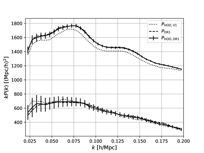
Figure 1: Validation of the DR1-like power spectrum (solid) for the best-fit LRG HOD model, A0. The DR1-like power spectrum is created by applying the DR1 window to the cubic mock (dotted). The DR1 window has been created with FFA effects included and $\theta$-cut applied. The true DR1 mock (dashed) is provided for comparison. Uncertainties are determined using a DR1 Gaussian covariance.

In order to explore relevant HOD-dependent effects for DR1, realistic data is a requirement (more discussion on this is in Section 4.2). Mocks generated with a single, fixed HOD that incorporate DR1 survey geometry and selection effects have been utilised extensively for systematic tests [54]. To explore HOD-dependent systematics in the context of DR1, rather than taking the computationally expensive approach of creating mocks with survey effects included for each HOD model, we instead produced what we will refer to as “DR1-like” data vectors. These DR1-like measurements are generated directly from the power spectrum measured on cubic mocks and only require a simple window convolution to mimic the full mock-based approach. These measurements are inexpensive to produce and could therefore be generated for each LRG, ELG and QSO HOD model. The mean of 25 mocks was used to create a “mock theory” vector, $\hat{P}_{\ell}^{t}(k^{\prime})$, which was then convolved with the realistic DR1 window matrix, $\mathsf{W}$, that captures the effect of fibre assignment estimated using the “fast-fibreassign” method (FFA; [55, 14]) and the effect of the $\theta$-cut. The $\theta$-cut, discussed in [56], is imposed to mitigate fibre assignment effects by removing pairs at small angular separations. It thus induces a sensitivity of the window to high-$k$ modes and therefore a basis rotation has also been applied in order to increase the compactness of the window as discussed in Section 10.1.2 of [14]. In Fourier-space, this convolution takes the form

$$\hat{P}_{\ell}^{\mathrm{DR1}}(k)=W_{\ell\ell^{\prime}}(k,k^{\prime})\hat{P}_{\ell}^{t}(k^{\prime}),$$ (3.1)

where $k^{\prime}$ and $k$ denote the input and output wavenumbers, respectively. The input multipoles extend to the hexadecapole, $\ell^{\prime}=(0,2,4)$, while the output was computed only up to the quadrupole, $\ell=(0,2)$. The window matrices correspond to a redshift binning with limits $z=[0.6,0.8],[1.1,1.6],[0.8,2.1]$ for the LRG, ELG and QSO samples, respectively. Only a single redshift bin for the LRG and ELG samples was used due to the computational cost required to produce covariance matrices for each HOD model (see Section 3.4). A single bin per tracer is sufficient for the purpose of this work given that we do not expect the effect of nuisance parameter priors, investigated using these data vectors, to change significantly across bins of a given tracer. The fitting process, described in Section 4.1, scales stochastic term priors by the shot-noise of the input data. To ensure that this scaling is correct relative to DR1 data (not the cubic box input $P(k)$), the newly-generated, DR1-like pypower files were assigned a shot-noise value equal to that of the fixed HOD DR1 mocks. Figure 1 demonstrates excellent agreement between the DR1-like data vector for the best-fit LRG model, A0, and the fixed HOD DR1 mock. DR1-like data vectors were not generated for the BGS tracer as we did not have the required number of realisations to reduce sample variance in estimating $\hat{P}_{\ell}^{t}(k^{\prime})$.

Throughout the rest of the paper, we will use the following terminology when denoting the type of data vector used:

• Cubic: Power spectrum measured on individual realisations of the AbacusSummit cubic box populated with all HOD models. Fits to this power spectrum are performed with the analytic V1 covariance corresponding to a single $(2\ \text{Gpc}\,h^{-1})^{3}$ cubic box.

• DR1-like: Power spectrum measured on the mean of 25 realisations of the AbacusSummit cubic box convolved with DR1 window. These are generated for each HOD model. Fits to this power spectrum are performed with the analytic covariance corresponding to the DR1 volume.

• Fixed HOD DR1: Power spectrum measured on mocks that incorporate survey geometry and selection effects. Only available for a single HOD model corresponding to the one that represents the best match to the DESI DR1 clustering.

More details on the cubic and fixed HOD DR1 mocks can be found in Section 11 of [14]. The analytic covariance matrices are described in the next section.

3.4 Covariance matrices

For the DR1 analysis, covariance matrices are constructed from 1000 effective Zel’dovich approximate mock simulations (EZmocks; [57]). These large $(6\ \text{Gpc}\,h^{-1})^{3}$ mocks allow the survey geometry of the DR1 sample to be reproduced without replication of the simulation box. In this work, we aim to produce covariance matrices that are tuned to the clustering of each HOD but roughly reproduce the DR1 EZmock covariance in the case of fits to the DR1-like data. For this reason, we compute analytic Fourier-space covariance matrices for each HOD model using the DESI Gaussian covariance code thecov [58]. This code follows the groundwork of [59] and [60] allowing the computation of power spectrum covariance matrices in arbitrary geometries. Covariance matrices are generated for both the V1 and DR1 volumes. The analytic approach used here makes the assumption of Gaussianity and so may underestimate the true covariance. The performance of the analytic covariance is validated against the EZmocks in [61], who find that the variance is slightly lower than that observed in the EZmocks. However, for the purpose of this work, the performance of the analytic covariance is sufficient. Section 10.2 in [14] details that the EZmocks are unable to reproduce the variance of the real data due to shortcomings in the FFA approximation. In order to account for this, a rescaling factor for each tracer is applied to the EZmocks based on their mismatch with the configuration-space DR1 covariance [62]. To obtain analytic covariances that match the variance of the data, we also apply these factors in this work.

The V1 covariance is easily generated by passing the cubic box power spectrum as input. In the case of DR1-like HOD mocks, a catalogue of random positions must be provided in addition to the cubic box power spectrum to account for survey geometry and selection effects. The random catalogue spans the survey footprint of the chosen tracer and samples the selection function of the data to ensure that no spurious clustering signal is measured when estimating the power spectrum. The random sample has also been subject to the FFA algorithm to mimic realistic fibre assignment effects. The catalogues correspond to the same redshift binning as the window matrices in Section 3.3. Once the analytic covariance matrix, $\mathsf{C}$, has been produced, a rotation (again following Section 10.1.2 of [14]) is applied,

$$\mathsf{C}^{\prime}=\mathsf{M}\mathsf{C}\mathsf{M}^{T},$$ (3.2)

where rotation matrix $\mathsf{M}$ is determined according to [56]. To reproduce the variance of the data, we correct the matrices with the corresponding rescaling factors, listed in Table 7 of [14], as discussed earlier. Additionally, a factor of $1.5$, obtained by roughly matching to the DR1 EZmock covariance, is applied to the ELG covariance in order to account for a discrepancy due to the fact that the input cubic box power spectrum is not at the redshift of the EZmocks. These factors are applied consistently to all HOD models of a given tracer.

4 Method

The full-shape analysis performed in BOSS and eBOSS (e.g., [63, 64, 65]) was based on a template-fitting approach which provided constraints on a set of summary parameters, a form of data compression. Cosmological results were then obtained in a subsequent step, through fitting models to the summary parameters assuming a Gaussian likelihood. This two-step process lent itself to expressing systematic error contributions in the form of an additional uncertainty in the results for the compressed parameters, which can be added in quadrature to the statistical errors and thus automatically propagated to cosmological parameter results in any model or in combination with any external data.

However, as detailed in [19], for the DESI DR1 results we use a full EFT-based approach, referred to as Full Modelling, in which cosmological parameters are fit directly from the data, in preference to the two-step template-based compression. While this has many benefits, it complicates the inclusion of possible systematic error contributions to the final error budget at the parameter-level as before, since the shifts obtained on any parameter depend both on the choice of which parameters are varied in the analysis and which external datasets, if any, are included in the fit alongside the galaxy power spectrum. Adding systematic error contributions at the parameter-level as before would thus require a separate estimate of the systematic uncertainty for each cosmological model and each combination of datasets that is to be considered—a prohibitive task.

Therefore, we propose to take a different approach: we quantify the effects of the systematic errors in terms of an additional effective uncertainty at the level of the power spectrum data vector, as explained in Section 4.2 below. This is expressed in the form of an additional covariance matrix contribution, $\mathsf{C}_{\rm sys}$, where the subscript here reflects that the source of this contribution is systematic. $\mathsf{C}_{\rm sys}$ is to be added (together with any other similar contributions from other sources) to the covariance matrix $\mathsf{C}_{\rm stat}$ representing the statistical measurement uncertainties in the power spectrum when performing a fit to the data, in order to capture the effect of systematic uncertainty in broadening posteriors in any parameter. Such an approach will then be generally applicable irrespective of which model parameters are held fixed or varied, or which additional datasets are included in the fits.

4.1 Model

All modelling and fitting routines used in this work are included within the DESI pipeline for likelihood analysis, desilike. We use the implementation of the velocileptors Lagrangian Perturbation Theory (LPT) code [66, 67] as our choice of EFT model to compute the redshift-space power spectrum monopole and quadrupole following the baseline parametrisation of [18]. Our choice of model here is arbitrary given the consistency of the DESI EFT codes [28]. The model computes perturbations up to 1-loop order and its performance has been validated on AbacusSummit mocks with a fixed HOD model in [28, 29]. The baseline for the DESI full-shape analysis investigates five varied cosmological parameters—although little information can be gained from the baryon density, $\omega_{b}$, as it is not constrained by the data and requires a prior which, in this work, is derived from Big Bang Nucleosynthesis (BBN) constraints [68]. For this reason, we choose to exclude $\omega_{b}$ from any figures. The prior on the scalar spectral index, $n_{s}$, is a Gaussian centred at $n_{s}=0.9649$ with a width chosen to be $10\times$ the posterior uncertainty from Planck [51]. The model includes two nuisance parameters per power spectrum multipole, counterterms $\alpha$ and stochastic terms SN, and three varied galaxy bias parameters. Counterterms and stochastic terms provide an additional contribution on top of the 1-loop power spectrum $P_{\mathrm{s,g}}^{\mathrm{PT}}$, leading to the redshift-space power spectrum,

$$P_{\mathrm{s,g}}(k,\mu)=P_{\mathrm{s,g}}^{\mathrm{PT}}(k,\mu)+(b_{1}+f\mu^{2})(b_{1}\alpha_{0}+f\alpha_{2}\mu^{2})k^{2}P_{\mathrm{s,lin}}(k,\mu)+(\mathrm{SN}_{0}+\mathrm{SN}_{2}k^{2}\mu^{2}),$$ (4.1)

where $P_{\mathrm{s,lin}}$ is related to the linear power spectrum, $f$ is the linear growth rate and $\mu$ is the cosine of the angle between wavevector $k$ and the line of sight (see [29] for further details). Allowing $b_{1}$ (linear), $b_{2}$ (quadratic) and $b_{s}$ (shear) bias terms to vary grants maximum flexibility of the model to marginalise over uncertainties in the galaxy-halo connection. The third order bias term $b_{3}$ is fixed due to degeneracies with the counterterms following [18]. The prior choices for all 12 varied parameters are listed in Table 1.

Cosmological	Prior	Nuisance	Prior
$\omega_{\mathrm{cdm}}$	$\mathcal{U}$[0.01, 0.99]	$(1+b_{1})\sigma_{8}$	$\mathcal{U}$[0, 3]
$\omega_{\mathrm{b}}$	$\mathcal{N}$[0.02237, 0.00055]	$b_{2}\sigma_{8}^{2}$	$\mathcal{N}$[0, 5]
$h$	$\mathcal{U}$[0.1, 10]	$b_{s}\sigma_{8}^{2}$	$\mathcal{N}$[0, 5]
ln($10^{10}A_{s}$)	$\mathcal{U}$[1.61, 3.91]	$\alpha_{0}^{p}$	$\mathcal{N}$[0, 12.5]
$n_{s}$	$\mathcal{N}$[0.9649, 0.04]	$\alpha_{2}^{p}$	$\mathcal{N}$[0, 12.5]
		SN${}_{0}^{p}$	$\mathcal{N}[0,2]\times 1/\bar{n}_{g}$
		SN${}_{2}^{p}$	$\mathcal{N}[0,5]\times f_{\rm sat}\sigma_{v}^{2}/\bar{n}_{g}$

Table 1: velocileptors LPT varied parameters and priors used for fitting. The entries $\mathcal{U}$[min, max] and $\mathcal{N}$[$\mu$, $\sigma$] refer to uniform and Gaussian normal distributions, respectively. Non-cosmological (nuisance) priors have been applied according to a “physically motivated” parametrisation following [29]. In this basis, counterterms scale relative to the linear theory multipoles and stochastic terms scale with the Poissonian shot-noise, $1/\bar{n}_{g}$, and the characteristic halo velocity dispersion, $f_{\rm sat}\sigma_{v}^{2}/\bar{n}_{g}$, where $f_{\rm sat}$ and $\sigma_{v}$ are the expected fraction and mean velocity dispersion of satellite galaxies, respectively. In the case of “uninformative” priors, infinite flat priors are instead imposed on nuisance parameters.

We investigate the effect of our physically motivated nuisance term priors by exploring shifts in the maximum a posteriori (MAP) value when flat priors are imposed on bias and nuisance terms. This case is equivalent to a maximum likelihood analysis, however the wide bounds on cosmological parameters are kept to ensure stability of the emulated model. We will refer to these different prior cases as “physical” and “uninformative”.

The model is emulated using a fourth-order Taylor expansion to increase the computational efficiency of the fitting procedure. This model is fit to the monopole and quadrupole over the range $k=0.02-0.2\ h\,\text{Mpc}^{-1}$ using the desilike wrapper of the Minuit profiler [69] to determine the MAP values. We choose not to employ Markov Chain Monte Carlo (MCMC) sampling when computing the HOD systematic contribution to avoid the inclusion of projection effects (see [18] for a discussion on this effect) which affect the posterior mean but not the MAP. However, in figures where we compare MAP values to the marginalised posterior, we employ the Hamiltonian Monte Carlo sampling algorithm NUTS [70, 71] to compute this. In this case, the linear nuisance parameters of our model, $\alpha$ and SN, have been analytically marginalised to accelerate sampling.

4.2 Estimating the systematic contribution

This work aims to capture two independent contributions at the level of the power spectrum:

1. The variation in HOD models that cannot be marginalised over by changing the nuisance parameters of our model. Given that the statistical covariance is computed with a fixed galaxy-halo connection, this additional contribution covers uncertainty in allowing this connection to vary.

2. The ability of the EFT model to fit the set of varied-HOD mocks given the allowed prior volume.

In order to address the first point, we can generate a covariance matrix directly from the variation in the measured summary statistic of interest. For the purpose of this work, we focus on the power spectrum. Using the power spectrum measurements discussed in Section 3.2, we can determine the residual,

$$\boldsymbol{\Delta P}^{\mathrm{A,B}}_{i}\equiv\boldsymbol{\hat{P}}^{\mathrm{A}}_{i}-\boldsymbol{\hat{P}}^{\mathrm{B}}_{i},$$ (4.2)

of HOD models A and B for a given tracer at fixed mock realisation $i$. Note that differences are only computed between HOD models corresponding to the same realisation to ensure that any non-HOD-dependent noise is excluded without the need to average measurements over all 25 realisations. We find this approach to be far more conservative due to the inclusion of stochastic effects of the HOD that would otherwise be lost. While the magnitude of these residuals depends on the range of HOD models explored, Figure 8 in Appendix A demonstrates that we explore an extremely conservative HOD prior space in matching to only the small-scale clustering. In this work, these measurements have been obtained with a fixed $\Lambda$CDM cosmology but, in theory, variations across a wide range of cosmologies could be accounted for in an equivalent manner. However, we expect the cosmological dependency to be weak as Eq. 4.2 computes relative shifts between models at a given cosmology. Additionally, changing the cosmology cannot drastically affect the HOD mock measurements as they must still roughly reproduce the observed clustering of the data. From this, we compute the covariance matrix

$$\mathsf{C}^{\rm V1}_{\mathrm{HOD}}=\mathrm{Cov}\big{[}\boldsymbol{\Delta P},\boldsymbol{\Delta P}\big{]}\,,$$ (4.3)

where

$$\boldsymbol{\Delta P}\equiv\big{\{}\boldsymbol{\Delta P}^{\mathrm{A,B}}_{i}\big{\}}_{\mathrm{A}\neq\mathrm{B}}\,\text{, for all permutations of A, B and $i$.}$$ (4.4)

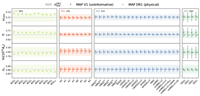
Figure 2: Best-fit cosmological parameters for different HOD models measured on cubic mocks with V1 covariance (V1) and DR1-like data with DR1 covariance (DR1). Fits to V1 have flat “uninformative” priors on nuisance terms such that differences between these points and those in the baseline “physical” parametrisation are due to the miscentering of priors—referred to as the “prior weight effect”. The coloured bands show the DR1 statistical uncertainty for each tracer at the redshift of the data (including EZmock rescaling). The error-bars show the standard deviation of 25 mock realisations. DR1-like data is generated from a power spectrum measurement averaged over 25 mocks, hence no error-bars are provided. Only one mock realisation is available for the BGS sample and so only one value corresponding to a single fit to V1 is shown.

This covariance matrix captures all of the variation in the measured mock power spectra due to the different galaxy-halo connection models within the wide, conservative HOD parameter space we explore, but does not include any effects of sample variance in the underlying halo catalogues themselves by construction (since differences are always computed at the same simulation realisation). Since the HOD models can vary substantially in quantities such as the effective galaxy biases which produce coherent shifts in the power spectra (see Figure 8 in Appendix A), this means that the differences in general are large, but the covariance matrix has a highly non-diagonal structure, especially in the monopole. Although individual terms in this covariance can be significantly larger than those of the statistical covariance, $\mathsf{C}_{\rm stat}$, strongly correlated differences like this are expected to be accommodated within the bias and nuisance terms of the EFT model. Therefore, although $\mathsf{C}^{\rm V1}_{\mathrm{HOD}}$ defined as above would dominate the total covariance, $\mathsf{C}^{\rm V1}_{\mathrm{tot}}=\mathsf{C}^{\rm V1}_{\mathrm{stat}}+\mathsf{C}^{\rm V1}_{\mathrm{HOD}}$, the effect of including this term on the posterior constraints on cosmological parameters of interest will be small—indeed, if the model is flexible enough to perfectly accommodate such HOD variations without biases in the cosmological parameters, the net effect will be zero. On the other hand, since the performance of the velocileptors model has only been validated on mock data generated with a single HOD model [29, 28] (and see also [30, 31] for equivalent models), this extra covariance term allows us to incorporate any potential additional variations to cosmological parameter constraints that might arise in the context of other HOD scenarios.

The covariance $\mathsf{C}^{\rm V1}_{\mathrm{HOD}}$ determined above makes no reference to the specific theory model of the power spectrum or the choice of which cosmological parameters are varied in any fit, so is generally valid for use in a wide array of contexts. However, it is large and very far from diagonal in structure, which is inconvenient and leads to concerns about the numerical precision with which its elements can be determined from a small number of simulation realisations. We therefore develop another alternative approach, in which the power spectrum residuals in Eq. 4.2 are instead replaced with

$$\boldsymbol{\Delta P}^{\mathrm{A,B}}_{i}\equiv\boldsymbol{P}_{i}(\vec{\Omega}_{\mathrm{A}},\vec{n}_{\it{bf}})-\boldsymbol{P}_{i}(\vec{\Omega}_{\mathrm{B}},\vec{n}_{\it{bf}}),$$ (4.5)

where power spectra $\boldsymbol{P}_{i}(\vec{\Omega}_{\mathrm{X}},\vec{n}_{\it{bf}})$ represent the theory prediction of the model evaluated at cosmological parameters, $\vec{\Omega}_{\mathrm{X}}$, at the MAP location for the fit to the measured power spectrum for given HOD model X, and at fixed nuisance parameters, $\vec{n}_{\it{bf}}$, corresponding to those at the MAP location for the fit to the power spectrum data for a single HOD model, chosen to be the one that represents the best match to the DESI clustering (e.g. model A0 for LRGs). The values $\vec{\Omega}_{\mathrm{X}}$ and $\vec{n}_{\it{bf}}$ were determined using the analytic covariance corresponding to the V1 volume for each model described in Section 3.4 with both cosmological and nuisance parameters freely varied. This alternative method removes the contributions to $\boldsymbol{\Delta P}^{\mathrm{A,B}}_{i}(k)$ that are highly correlated in $k$ and are effectively absorbed by the nuisance parameters in any fit, thus isolating only the effects of the HOD variation leading to shifts in the cosmologically-relevant parameters. This leads to a much smaller and more diagonal $\mathsf{C}^{\rm V1}_{\rm HOD}$, with the total $\mathsf{C}^{\rm V1}_{\rm tot}$ now dominated by the usual statistical term and less sensitive to the precision of the determination of the HOD contribution. However, since the determination of the MAP values and the evaluation of $P_{i}(\vec{\Omega}_{\mathrm{X}},\vec{n}_{\it{bf}})$ is done within the context of a cosmological model (in our case, flat $\Lambda$CDM with fixed neutrino mass sum $\sum m_{\nu}=0.06$ eV), the result is not as general as in the first approach. In light of this, we investigate the effect in $w$CDM in Appendix B and find it to be negligible given the increased statistical errors.

In Appendix A, we compare the two approaches in terms of their effects on the final posteriors on cosmological parameters of interest and show that they produce very similar results, with the second approach giving a slightly conservative estimate of the total sensitivity to the unknown galaxy-halo connection in this case. For this reason, and because of its relative simplicity, we present our default results using the second approach, which we refer to as the “approximate” approach. However, for future DESI analyses this choice may be revisited.

Figure 2 shows the mean and standard deviation of cosmological parameter MAP values across the mocks for each of the models considered. Both fits to individual realisations of the cubic box with corresponding V1 covariance and fits to the DR1-like power spectrum with covariance corresponding to the DR1 volume (see Sections 3.3 and 3.4) are shown. For variations in the HOD, we are only interested the “V1 MAP (uninformative)” case—fits to the cubic box with the flat nuisance parameters.

	std($x_{\mathrm{A,i}}-x_{\mathrm{B,i}}$) (% $\sigma^{\mathrm{DR1}}_{\mathrm{stat}}$)
Tracer	$\omega_{\mathrm{cdm}}$	$h$	ln($10^{10}A_{s}$)	$n_{s}$
BGS	8.4	6.3	7.5	7.5
LRG	20.8	18.3	22.7	12.0
ELG	31.3	20.7	26.8	26.0
QSO	42.5	46.1	63.8	7.8

Table 2: Standard deviation of parameter-level shifts in MAP (uninformative) values between V1 cubic HOD mocks. The shifts are quoted relative to the DR1 statistical error (including EZmock rescaling) at the redshift of the data.

Computing the covariance over all permutations of models A and B allows for increased statistical power. We acknowledge that the covariance of shifts in the data vector between different HOD models (Eq. 4.5) is not necessarily a true estimate of the covariance between the models themselves. According to the Cauchy-Schwarz inequality, this estimate of the variance, $\sigma^{2}_{\mathrm{A-B}}$, must lie somewhere in the range $0<\sigma^{2}_{\mathrm{A-B}}<4\sigma^{2}_{\mathrm{A}}$ depending on the level of correlation between models. However, to ensure that our method does not underestimate the systematic contribution, we have verified that

$$\mathrm{Var}\big{[}\boldsymbol{P}_{i}(\vec{\Omega}_{\mathrm{A}},\vec{n}_{\it{bf}})-\boldsymbol{P}_{i}(\vec{\Omega}_{\mathrm{B}},\vec{n}_{\it{bf}})\big{]}\geq\mathrm{Var}\big{[}\boldsymbol{P}_{i}(\vec{\Omega}_{\mathrm{A}},\vec{n}_{\it{bf}})-\boldsymbol{P}_{i}(\vec{\Omega}_{\it{bf}},\vec{n}_{\it{bf}})\big{]}$$ (4.6)

holds on average across the $k$-range of interest. The largest violation occurs at high $k$ in the ELG monopole where the variance appears to be underestimated by a factor of $\sim 0.8$. We therefore believe that the systematic estimate presented is conservative, providing an upper bound on the HOD systematic contribution.

Due to the low number of available mocks for BGS and QSO, these models are combined with the LRGs to produce a more accurate covariance. We believe this to be well-motivated given the similarity in the form of their HODs. The best-fit cosmology for the LRG models is used to create supplementary synthetic data vectors at the corresponding BGS and QSO redshifts. When iterating over permutations in Eq. 4.4, we ensure that cases where models A and B belong to different tracers are not included as they have been tuned to different clustering measurements.

Finally, in order to investigate the effect on DR1 data, we apply the DR1 window matrix, $\mathsf{W}$, described in Section 3.3, to the covariance matrix,

$$C^{\rm DR1}_{\mathrm{HOD}}(k,k)=W(k,k^{\prime})C^{\rm V1}_{\mathrm{HOD}}(k^{\prime},k^{\prime})W(k,k^{\prime})^{\mathrm{T}}.$$ (4.7)

For this reason, $\mathsf{C}^{\rm V1}_{\mathrm{HOD}}$ is computed up to $k^{\prime}=0.35\ h\,\text{Mpc}^{-1}$, the maximum wavenumber used in the window convolution.

The modelling systematic has been shown to be negligible for a $(2\ \text{Gpc}\,h^{-1})^{3}$ cubic mock populated with a single, fixed HOD [28]; however, the DR1 data samples have smaller effective volume and thus lower statistical power than these boxes, so the effect of prior choices can be different. The second point above can be considered an extension of this analysis, not only in terms of other models, but also including effects specific to the DR1 analysis that influence the contribution of priors. Given the constraining power of DR1, physically-motivated priors are imposed on nuisance parameters to mitigate projection effects. The physically-motivated stochastic term priors are dependent on the tracer density. Both the increase in the sample variance and prior dependence on the tracer density will change the weight of the prior relative to the likelihood and may systematically shift the MAP value in a HOD-dependent way. This shifting of the MAP value due to the miscentering of priors we refer to as the “prior weight effect” and can be observed in Figure 2. This necessitates the need for analyses with realistic DR1 number density and covariance. To capture all of these effects, we compute an additional diagonal contribution to the covariance

$$\boldsymbol{D}_{\mathrm{model}}=\mathrm{max}\big{(}\big{\{}\boldsymbol{\delta P}^{\mathrm{A}}\big{\}})^{2},$$ (4.8)

from our DR1-like data where

$$\boldsymbol{\delta P}^{\mathrm{A}}\equiv\boldsymbol{\hat{P}}^{\mathrm{A}}_{\mathrm{DR1}}-\boldsymbol{P}^{\mathrm{A}}_{\mathrm{MAP}}.$$ (4.9)

The maximum residual between the DR1-like window-convolved power spectrum $\boldsymbol{\hat{P}}^{\mathrm{A}}_{\mathrm{DR1}}$ and the theory model evaluated at the best-fit MAP values $\boldsymbol{P}^{\mathrm{A}}_{\mathrm{MAP}}$ is computed at each value of $k$ over all HOD models, $\{\mathrm{A}\}$. The MAP fit is performed using the DR1 covariance described in Section 3.4. In the case of the BGS, $\boldsymbol{D}_{\mathrm{model}}$ cannot practically be computed as we only have access to a single realisation, so we instead assume that it is equal to the equivalent contribution estimated for the LRGs.

The total HOD-dependent contribution to the covariance is therefore given by

$$\mathsf{C}_{\rm sys}=\mathsf{C}^{\rm DR1}_{\mathrm{HOD}}+\mathrm{diag}(\boldsymbol{D}_{\mathrm{model}}).$$ (4.10)

5 Results

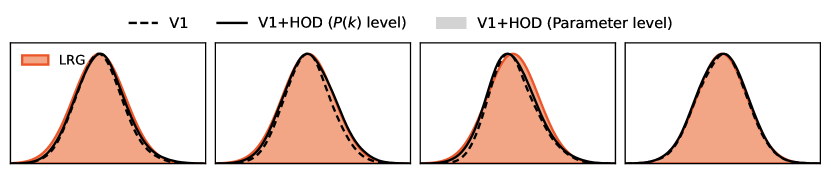
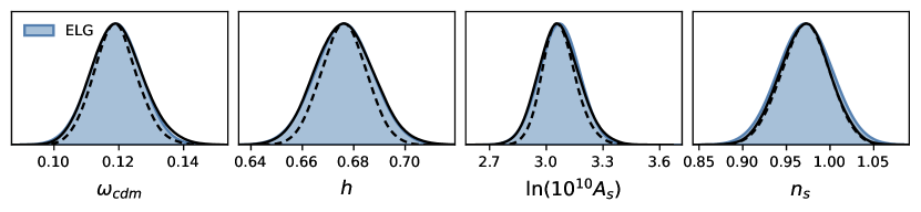
Figure 3: Parameter posteriors when HOD systematics are added at the parameter-level (filled) versus at the data-level (solid) for LRG (red) and ELG (blue) tracer samples. Fits are performed to the V1 cubic mock populated with the best-fit HOD model for each tracer. The V1-only posterior (no HOD contribution) is given as a dashed line for comparison. The relative HOD contribution is significantly greater in the case of V1 than compared to DR1 data due to the large increase in volume. The posterior on $n_{s}$ is prior-dominated and we therefore do not expect to see any change with the HOD contribution included at the $P(k)$-level.

5.1 Comparison to parameter-level estimates

In Figure 3, we show the comparison between adding a HOD-dependent systematic contribution at the level of the parameters—computed as described below—and at the level of the power spectrum. The two approaches are compared in the context of the V1 cubic box volume rather than the reduced volume of DR1 in order to more easily distinguish the HOD contribution from the statistical error. To show the combined V1+HOD uncertainty at the parameter-level, we generate a Gaussian distribution centred at the posterior mean of a fit to the mean power spectrum obtained from 25 realisations of the V1 best-fit HOD cubic mock. The posterior width, $\sigma^{\mathrm{V1}}_{\mathrm{stat}}$, is then inflated by the HOD contribution in quadrature,

$$(\sigma^{x}_{\mathrm{comb}})^{2}=(\sigma^{\mathrm{V1}}_{\mathrm{stat}})^{2}+(\sigma^{\mathrm{V1}}_{\mathrm{HOD}})^{2}+\mathrm{diag}(\bar{x}^{p}-\bar{x}^{\mathrm{flat}})^{2}$$ (5.1)

where $x$ is the cosmological parameter of interest and $\bar{x}^{p}$ and $\bar{x}^{\mathrm{flat}}$ are the MAP values fit to the mean of 25 mocks with physical and uninformative nuisance priors, respectively. The diagonal contribution captures the prior weight effect (given the V1 volume) in a similar manner to Eq. 4.9 while the contribution from HOD-dependent shifts in cosmology,

$$\sigma^{\mathrm{V1}}_{\mathrm{HOD}}\equiv\mathrm{std}\big{(}\{x^{\mathrm{A}}_{i}-x^{\mathrm{B}}_{i}\}_{\mathrm{A}\neq\mathrm{B}}\big{)},$$ (5.2)

are listed in Table 2. Here, $x^{\mathrm{X}}_{i}$ denotes the MAP values of HOD model X fit to mock realisation $i$ with uninformative nuisance priors. In this comparison, the V1 analytic covariances were used throughout. The posterior with the HOD contribution added at the level of the power spectrum, as in our fiducial analysis described in the previous section, is shown for comparison. To produce this posterior, the Gaussian covariance was combined with the unwindowed HOD contribution (Eq. 4.3) including a diagonal contribution equivalent to that of Eq. 4.8, except that the residual between best-fit model and data (Eq. 4.9) was determined from a fit to the mean power spectrum obtained from 25 cubic box mock realisations using the V1 analytic covariance. The figure shows exceptional agreement between the two cases demonstrating that both the inability of the model to absorb changes in the galaxy-halo connection and the impact of the priors on nuisance parameters are correctly accounted for. The additional diagonal contribution to the HOD covariance captures the effect of the nuisance priors in a trivial way—shifts in the MAP value are simply translated into the ability of the model to fit the data with the chosen priors.

5.2 DR1 HOD covariance

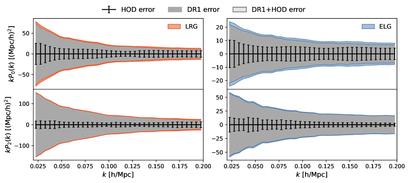
Figure 4: Contribution of HOD systematics to the diagonal of the DR1 EZmock covariance matrix.

With the covariance validated on the cubic mocks, we present results for the final DR1 windowed covariance. Figure 4 shows the additional contribution to the EZmock covariance diagonal. The EZmock rescaling, discussed in Section 3.4, is not applied to make the HOD contribution more apparent. As expected, the uncertainty sourced by varying the galaxy-halo connection is most dominant at small scales relative to the statistical uncertainty. However, it is also evident that even the largest scales are impacted by the inability to completely marginalise over these small-scale effects. The full combined correlation matrices are shown in Figure 5. The HOD contribution has a higher degree of correlation than the EZmock statistical covariance but this off-diagonal contribution is subdominant to the diagonal of the statistical covariance and has no effect on the parameter correlation structure (see Figure 7 in Section 5.3).

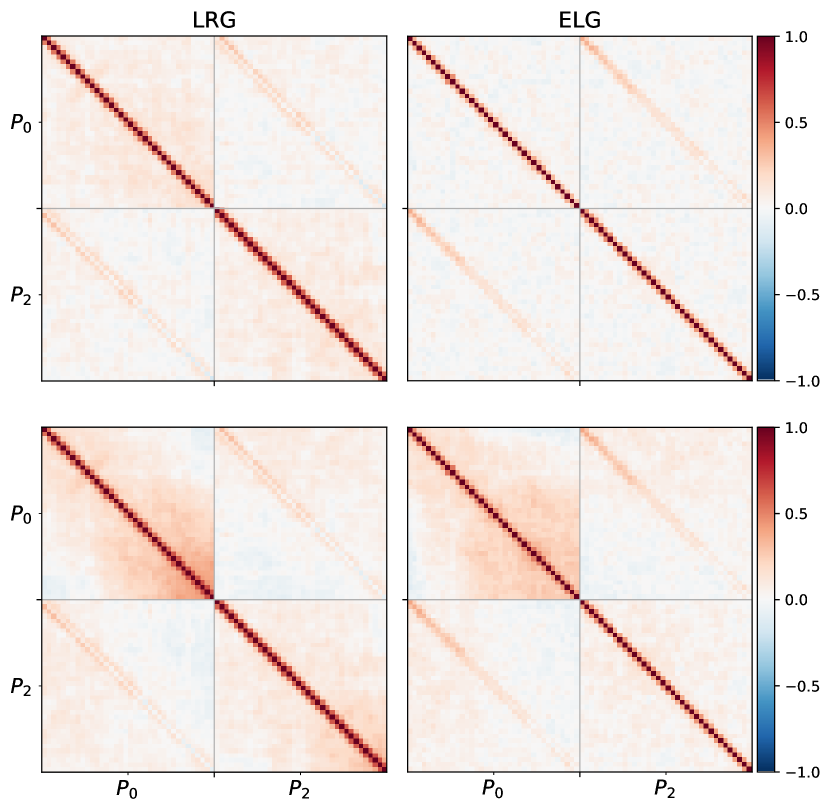
Figure 5: Correlation matrix for DR1 estimated from 1000 EZmocks (upper) and DR1+HOD combined (lower). Off-diagonal correlations are a result of the HOD-dependent contribution.

5.3 Combined covariance fits to DR1 mocks

The DESI 2024 full-shape analysis utilises the covariance matrices produced in this work, in combination with EZmock-based covariance matrices, in order to determine the full statistical plus systematic error. Mock-based covariance matrices have an intrinsic uncertainty in their estimate and also result in biased estimates of the inverse [72, 73, 74, 75]. To account for this, a correction factor, $f$ (see equation 56 in [76]; this is a generalisation of the Hartlap correction [72] to also propagate the uncertainty in the estimate of the covariance matrix to the derived parameter posteriors), is typically applied. We apply this correction only to the EZmock statistical covariance, $\mathsf{C}_{\rm stat}$, given that the expression

$$\langle(\mathsf{C}_{\rm stat}+\mathsf{C}_{\rm sys})^{-1}\rangle \approx\langle\mathsf{C}_{\rm stat}^{-1}\rangle-\langle\mathsf{C}_{\rm stat}^{-1}\rangle\mathsf{C}_{\rm sys}\langle\mathsf{C}_{\rm stat}^{-1}\rangle$$ (5.3)

$$\approx(f\mathsf{C}_{\rm stat}+\mathsf{C}_{\rm sys})^{-1}$$ (5.4)

holds to first order under the condition that $\mathsf{C}_{\rm sys}$ is a small contribution to $\mathsf{C}_{\rm stat}$. While this assumes that $\mathsf{C}_{\rm sys}$ is perfectly known, noise in the estimate of $\mathsf{C}_{\rm sys}$ should be negligible in terms of the total covariance.

Figure 6 shows that the effect of the additional HOD systematic covariance is minimal for fits to DR1 mocks. However, this will become more prevalent as the constraining power of the survey increases, becoming a significant contribution to the total error budget for a V1-like volume (see Figure 3). The mean values in Figure 6 have been plotted at the effective redshifts of the data for visualisation purposes. As we employ a full covariance treatment, the effect on the 2-dimensional posterior can also be explored in Figure 7. For the ELG tracer in the redshift range $z=1.1-1.6$, we show that the HOD contribution acts to inflate the cosmological parameter contours while maintaining the degeneracy structure.

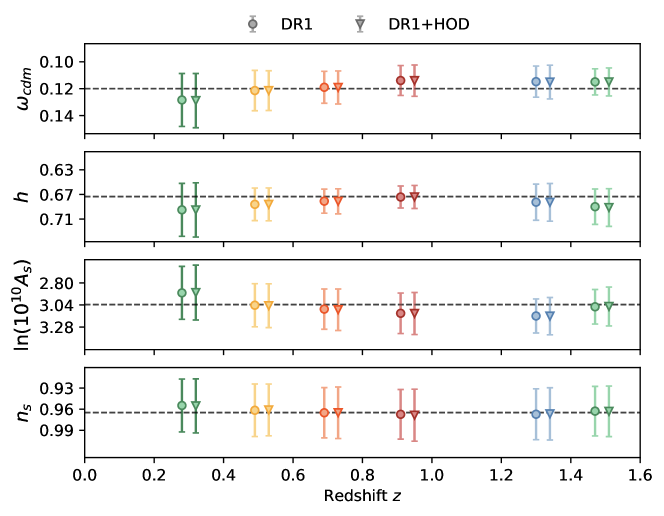
Figure 6: Effect of the HOD systematic contribution on fits to DR1 mocks. Mean and $1\sigma$ intervals are shown for each tracer and centred at the redshift of the data for visualisation purposes. The DR1 covariance is computed from 1000 EZmocks.

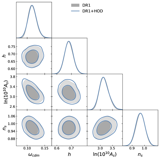
Figure 7: Cosmological parameter posteriors for the ELG DR1 mock at $z=1.1-1.6$. By utilising a full covariance treatment, our method of adding the HOD systematic contribution at the level of the data vector allows the effect on the 2D posterior to be shown. The effect on the posterior is minimal.

6 Conclusions

In this paper, we have studied the impact of varying the HOD on the DESI 2024 full-shape galaxy clustering analysis and present a new method for the inclusion of mock-based systematic estimates at the level of the data vector. By fitting an EFT model to a variety of HOD mocks for the four DESI tracers—BGS, LRG, ELG and QSO, we have produced systematic covariance matrices that reflect the HOD-dependent variation of the data vector. Additionally, our systematic covariance includes a contribution that captures the ability of the model to fit the HOD mocks given a set of informative nuisance parameter priors—naturally incorporating any uncertainty in our choice of prior. Our method has been validated against the parameter-level approach used formerly [32, 33], showing excellent consistency. The HOD systematic covariance matrices for each tracer are provided for the DESI 2024 full-shape analysis as an additional contribution to the statistical covariance.

At the parameter-level, changes in the HOD have been shown to shift the recovered cosmological parameters by greater than 20% of the DR1 statistical error (Table 2). This only induces a near-negligible inflation of the posterior width for each of the samples. However, we do expect this effect to become more important as the constraining power of the survey improves as evidenced by the effect on the $(2\ \text{Gpc}\,h^{-1})^{3}$ V1 cubic mocks (Figure 3).

Adding the systematic contribution at the level of the data vector has advantages. A full covariance treatment is more rigorous than simply inflating the statistical covariance by some factor or broadening uncertainties on the recovered parameters. The method is also more general and robust to choices of model free parameters or additional external datasets. The covariance matrices provided for the DESI 2024 full-shape analysis employ an approximate method to diagonalise and reduce sensitivity to the covariance (Eq. 4.5). The approximate method yields a more conservative estimate in $\Lambda$CDM but is less general given that extended models can introduce new degeneracies between cosmology and nuisance parameters. However, we show this effect to be negligible with respect to the DR1 statistical uncertainties in Appendix B. While we take the conservative approach and employ the approximate method for DR1, we may reconsider this choice in future data releases as the constraining power of the survey increases.

Incorporating the HOD-dependent systematic at the level of the data vector is a method that could be applied to other mock-based systematics tests provided a suitably large number of mocks are available. Given that this method is not suited for systematic tests with a low number of mocks, increasing the number of HOD mocks for the BGS and QSO samples is of high priority. Additionally, exploring the effects of varying the HOD in mocks created with non-$\Lambda$CDM base cosmologies is an essential step forward in light of results from DESI BAO [11]. While we expect the cosmological dependence of the HOD covariance to be small, our generalised method can be easily extended to include alternate cosmologies provided that a sufficient number of mocks are available.

Data Availability

Data from the plots in this paper will be available on Zenodo as part of DESI’s Data Management Plan. The data used in this analysis will be made public along with Data Release 1 (details in https://data.desi.lbl.gov/doc/releases/).

Appendix A Method consistency in $\Lambda$CDM

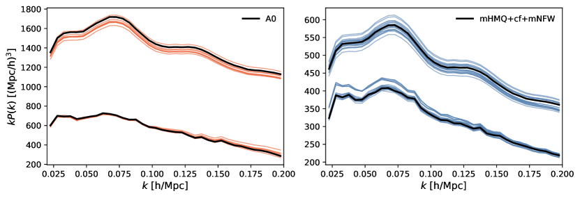
Figure 8: Power spectrum measurements of HOD-varied AbacusSummit cubic mocks (Section 3.2) averaged over 25 realisations for the LRG (left) and ELG (right) samples. Both the monopole and quadrupole are displayed. The best-fit HOD model is displayed in black.

In this work, we choose to take an approximate approach in the computation of the covariance matrix in order to produce a more diagonal and less sensitive covariance. In this approach, the nuisance parameters are fixed to the measured best-fit values corresponding to a single HOD model following Eq. 4.5. Without this, the covariance is large and highly non-diagonal due to the different effective galaxy biases of HOD mocks. This can be observed in Figure 8 where the mock power spectra, as described in Section 3.2, are shown. While these measurements have been tuned to the clustering of the One-Percent Survey on small scales, large-scale effects such as linear bias are not constrained leading to the large amplitude shift. Generating the covariance in this way also allows the inclusion of HOD models at different redshift which is advantageous given the dataset of ELG mocks. While this method is expected to produce the correct result in $\Lambda$CDM, it suffers from a loss of applicability to extended models (more on this in Appendix B). We do however still expect it to be more robust than parameter-level methods if only estimated in $\Lambda$CDM.

The generalised approach, following Eq. 4.2, produces a highly-correlated covariance matrix with a magnitude of the order of the statistical covariance. Given the large relative contribution to the total covariance, greater accuracy in estimating the correct correlation structure is required. One must also take care in applying covariance correction factors (see Section 5.3) to the, now non-negligible, HOD contribution. As we are using analytically-determined statistical covariance matrices, we instead apply correction factor $f$ to the HOD contribution only. This follows the same line of thought as Eq. 5.3 but instead treats $\mathsf{C}_{\rm stat}$ as perfectly known and accounts for noise in the estimate of $\mathsf{C}_{\rm HOD}$. Figure 9 shows that the number of mocks used in this work is sufficient to achieve equivalent posteriors with these approaches in $\Lambda$CDM.

Although we proceed with the approximate method for the DR1 analysis for robustness, we show that both methods are entirely consistent and motivate the full, general approach for future data releases.

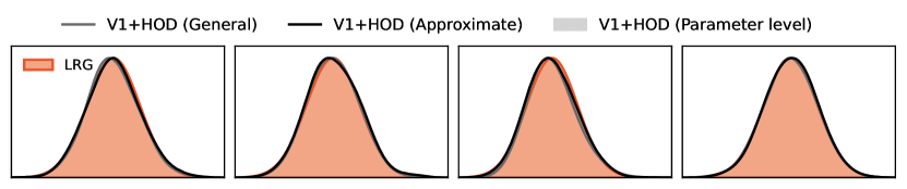
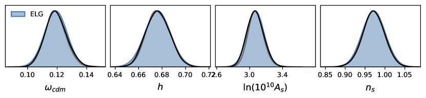
Figure 9: Comparison of the effect of using the HOD covariance matrix generated using the generalised approach (grey) and the approximate approach in which nuisance parameters are fixed (black). ELG models at $z=0.8$ and the diagonal contribution of Eq. 4.8 have not been included here for consistency. Both methods at the level of the data vector are able to reproduce the parameter-level HOD contribution of Eq. 5.1 without the diagonal contribution (filled).

Appendix B HOD-dependence and performance of approximate method in $w$CDM

In order to test the robustness of our method in extended cosmologies, we explore HOD-dependent systematics within the framework of the $w$CDM cosmological model. When the equation of state parameter, $w$, is allowed to vary, we find that the shifts in cosmological parameters between different HOD mocks are larger than in the $\Lambda$CDM case. Therefore, parameter-level methods to estimate HOD-dependent systematics are not transferable to other cosmological models in a trivial manner. If the approximate covariance method is used, this issue also persists at the level of the data vector—fixing the nuisance parameters in $w$CDM does not remove the highly correlated behaviour of the power spectrum monopole as it does in $\Lambda$CDM. While we believe the method is robust to the strong degeneracy between $w$ and $h$, the addition of new cosmological-nuisance degeneracies evidently inflates variations at the level of the data vector. This is due to the fact that fixing nuisance parameters in the estimation of the covariance can introduce unrealistic shifts in an extended model if there is a different coupling between nuisance parameters and cosmology. In simple terms, a change in this degeneracy means that an evaluation of the theory with only a change in cosmological parameters is not a physical representation of how that HOD would modify the data vector. However, this has no effect in the case that the coupling is unchanged from the model in which you measured the best-fit parameters. In Figure 10, we show that the effect on the posterior for the V1 cubic box is negligible for $w$CDM due to increased statistical uncertainty. Given that extended models are unlikely to be impacted by HOD-dependent systematics for DR1 due to the large statistical uncertainty, we motivate using the approximate method given that it is more conservative in $\Lambda$CDM.

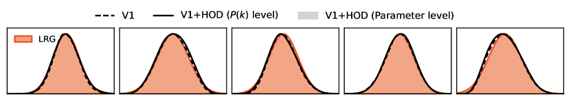
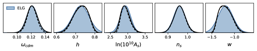
Figure 10: Same as Figure 3 except fits have been performed in $w$CDM. The additional HOD contribution has been determined in $\Lambda$CDM but we find this to be suitable for our purposes given that the relative contribution to the total error is far smaller in extended models. The filled contours are Gaussian curves and so do not reflect the non-Gaussianity of the true posteriors given by the solid and dashed lines.

Appendix C Author Affiliations

¹Institute of Cosmology and Gravitation, University of Portsmouth, Dennis Sciama Building, Portsmouth, PO1 3FX, UK

²Department of Physics and Astronomy, University of Waterloo, 200 University Ave W, Waterloo, ON N2L 3G1, Canada

³Perimeter Institute for Theoretical Physics, 31 Caroline St. North, Waterloo, ON N2L 2Y5, Canada

⁴Waterloo Centre for Astrophysics, University of Waterloo, 200 University Ave W, Waterloo, ON N2L 3G1, Canada

⁵IRFU, CEA, Université Paris-Saclay, F-91191 Gif-sur-Yvette, France

⁶Sorbonne Université, CNRS/IN2P3, Laboratoire de Physique Nucléaire et de Hautes Energies (LPNHE), FR-75005 Paris, France

⁷Departament de Física Quàntica i Astrofísica, Universitat de Barcelona, Martí i Franquès 1, E08028 Barcelona, Spain

⁸Institut d’Estudis Espacials de Catalunya (IEEC), 08034 Barcelona, Spain

⁹Institut de Ciències del Cosmos (ICCUB), Universitat de Barcelona (UB), c. Martí i Franquès, 1, 08028 Barcelona, Spain.

¹⁰University of Michigan, Ann Arbor, MI 48109, USA

¹¹Laboratoire de Physique Subatomique et de Cosmologie, 53 Avenue des Martyrs, 38000 Grenoble, France

¹²Center for Astrophysics $|$ Harvard & Smithsonian, 60 Garden Street, Cambridge, MA 02138, USA

¹³Department of Physics, The University of Texas at Dallas, Richardson, TX 75080, USA

¹⁴NASA Einstein Fellow

¹⁵Ecole Polytechnique Fédérale de Lausanne, CH-1015 Lausanne, Switzerland

¹⁶Physics Dept., Boston University, 590 Commonwealth Avenue, Boston, MA 02215, USA

¹⁷Dipartimento di Fisica “Aldo Pontremoli”, Università degli Studi di Milano, Via Celoria 16, I-20133 Milano, Italy

¹⁸Department of Physics & Astronomy, University College London, Gower Street, London, WC1E 6BT, UK

¹⁹Lawrence Berkeley National Laboratory, 1 Cyclotron Road, Berkeley, CA 94720, USA

²⁰Institute for Computational Cosmology, Department of Physics, Durham University, South Road, Durham DH1 3LE, UK

²¹Instituto de Física, Universidad Nacional Autónoma de México, Cd. de México C.P. 04510, México

²²NSF NOIRLab, 950 N. Cherry Ave., Tucson, AZ 85719, USA

²³Kavli Institute for Particle Astrophysics and Cosmology, Stanford University, Menlo Park, CA 94305, USA

²⁴SLAC National Accelerator Laboratory, Menlo Park, CA 94305, USA

²⁵Institut de Física d’Altes Energies (IFAE), The Barcelona Institute of Science and Technology, Campus UAB, 08193 Bellaterra Barcelona, Spain

²⁶Departamento de Física, Universidad de los Andes, Cra. 1 No. 18A-10, Edificio Ip, CP 111711, Bogotá, Colombia

²⁷Observatorio Astronómico, Universidad de los Andes, Cra. 1 No. 18A-10, Edificio H, CP 111711 Bogotá, Colombia

²⁸Institute of Space Sciences, ICE-CSIC, Campus UAB, Carrer de Can Magrans s/n, 08913 Bellaterra, Barcelona, Spain

²⁹Fermi National Accelerator Laboratory, PO Box 500, Batavia, IL 60510, USA

³⁰Department of Astrophysical Sciences, Princeton University, Princeton NJ 08544, USA

³¹Center for Cosmology and AstroParticle Physics, The Ohio State University, 191 West Woodruff Avenue, Columbus, OH 43210, USA

³²Department of Physics, The Ohio State University, 191 West Woodruff Avenue, Columbus, OH 43210, USA

³³The Ohio State University, Columbus, 43210 OH, USA

³⁴School of Mathematics and Physics, University of Queensland, 4072, Australia

³⁵Institució Catalana de Recerca i Estudis Avançats, Passeig de Lluís Companys, 23, 08010 Barcelona, Spain

³⁶Department of Physics and Astronomy, Siena College, 515 Loudon Road, Loudonville, NY 12211, USA

³⁷Departament de Física, EEBE, Universitat Politècnica de Catalunya, c/Eduard Maristany 10, 08930 Barcelona, Spain

³⁸Department of Physics and Astronomy, Sejong University, Seoul, 143-747, Korea

³⁹CIEMAT, Avenida Complutense 40, E-28040 Madrid, Spain

⁴⁰Department of Physics, University of Michigan, Ann Arbor, MI 48109, USA

⁴¹Department of Physics & Astronomy, Ohio University, Athens, OH 45701, USA

References

- [1] M. Levi, C. Bebek, T. Beers, R. Blum, R. Cahn, D. Eisenstein et al., The DESI Experiment, a whitepaper for Snowmass 2013, arXiv e-prints (2013) arXiv:1308.0847 [1308.0847].
- [2] DESI Collaboration, A. Aghamousa, J. Aguilar, S. Ahlen, S. Alam, L.E. Allen et al., The DESI Experiment Part I: Science,Targeting, and Survey Design, arXiv e-prints (2016) arXiv:1611.00036 [1611.00036].
- [3] DESI Collaboration, B. Abareshi, J. Aguilar, S. Ahlen, S. Alam, D.M. Alexander et al., Overview of the Instrumentation for the Dark Energy Spectroscopic Instrument, AJ 164 (2022) 207 [2205.10939].
- [4] DESI Collaboration, A. Aghamousa, J. Aguilar, S. Ahlen, S. Alam, L.E. Allen et al., The DESI Experiment Part II: Instrument Design, arXiv e-prints (2016) arXiv:1611.00037 [1611.00037].
- [5] J.H. Silber, P. Fagrelius, K. Fanning, M. Schubnell, J.N. Aguilar, S. Ahlen et al., The Robotic Multiobject Focal Plane System of the Dark Energy Spectroscopic Instrument (DESI), AJ 165 (2023) 9 [2205.09014].
- [6] T.N. Miller, P. Doel, G. Gutierrez, R. Besuner, D. Brooks, G. Gallo et al., The Optical Corrector for the Dark Energy Spectroscopic Instrument, AJ 168 (2024) 95 [2306.06310].
- [7] DESI Collaboration, A.G. Adame, J. Aguilar, S. Ahlen, S. Alam, G. Aldering et al., Validation of the Scientific Program for the Dark Energy Spectroscopic Instrument, AJ 167 (2024) 62 [2306.06307].
- [8] DESI Collaboration, A.G. Adame, J. Aguilar, S. Ahlen, S. Alam, G. Aldering et al., The Early Data Release of the Dark Energy Spectroscopic Instrument, AJ 168 (2024) 58 [2306.06308].
- [9] DESI Collaboration, A.G. Adame, J. Aguilar, S. Ahlen, S. Alam, D.M. Alexander et al., DESI 2024 III: Baryon Acoustic Oscillations from Galaxies and Quasars, arXiv e-prints (2024) arXiv:2404.03000 [2404.03000].
- [10] DESI Collaboration, A.G. Adame, J. Aguilar, S. Ahlen, S. Alam, D.M. Alexander et al., DESI 2024 IV: Baryon Acoustic Oscillations from the Lyman Alpha Forest, arXiv e-prints (2024) arXiv:2404.03001 [2404.03001].
- [11] DESI Collaboration, A.G. Adame, J. Aguilar, S. Ahlen, S. Alam, D.M. Alexander et al., DESI 2024 VI: Cosmological Constraints from the Measurements of Baryon Acoustic Oscillations, arXiv e-prints (2024) arXiv:2404.03002 [2404.03002].
- [12] E.F. Schlafly, D. Kirkby, D.J. Schlegel, A.D. Myers, A. Raichoor, K. Dawson et al., Survey Operations for the Dark Energy Spectroscopic Instrument, AJ 166 (2023) 259 [2306.06309].
- [13] J. Guy, S. Bailey, A. Kremin, S. Alam, D.M. Alexander, C. Allende Prieto et al., The Spectroscopic Data Processing Pipeline for the Dark Energy Spectroscopic Instrument, AJ 165 (2023) 144 [2209.14482].
- [14] DESI Collaboration, A.G. Adame, J. Aguilar, S. Ahlen, S. Alam, D.M. Alexander et al., DESI 2024 II: Sample Definitions, Characteristics, and Two-point Clustering Statistics, arXiv e-prints (2024) arXiv:2411.12020 [2411.12020].
- [15] C. Blake and K. Glazebrook, Probing Dark Energy Using Baryonic Oscillations in the Galaxy Power Spectrum as a Cosmological Ruler, ApJ 594 (2003) 665 [astro-ph/0301632].
- [16] H. Seo and D. Eisenstein, Probing Dark Energy with Baryonic Acoustic Oscillations from Future Large Galaxy Redshift Surveys, ApJ 598 (2003) 720 [astro-ph/0307460].
- [17] N. Kaiser, Clustering in real space and in redshift space, MNRAS 227 (1987) 1.
- [18] DESI Collaboration, A.G. Adame, J. Aguilar, S. Ahlen, S. Alam, D.M. Alexander et al., DESI 2024 V: Full-Shape Galaxy Clustering from Galaxies and Quasars, arXiv e-prints (2024) arXiv:2411.12021 [2411.12021].
- [19] DESI Collaboration, A.G. Adame, J. Aguilar, S. Ahlen, S. Alam, D.M. Alexander et al., DESI 2024 VII: Cosmological Constraints from the Full-Shape Modeling of Clustering Measurements, arXiv e-prints (2024) arXiv:2411.12022 [2411.12022].
- [20] S. Ramirez-Solano, M. Icaza-Lizaola, H.E. Noriega, M. Vargas-Magaña, S. Fromenteau, A. Aviles et al., Full modeling and parameter compression methods in configuration space for desi 2024 and beyond, arXiv e-prints (2024) arXiv:2404.07268 [2404.07268].
- [21] E. Chaussidon et al., Constraining the local primordial non-gaussianity via the large scale-dependent bias with the DESI DR1 LRG and QSO, in preparation (2024) .
- [22] DESI Collaboration, DESI 2024 I: Data Release 1 of the Dark Energy Spectroscopic Instrument, in preparation (2025) .
- [23] R. Wechsler and J. Tinker, The Connection Between Galaxies and Their Dark Matter Halos, ARA&A 56 (2018) 435 [1804.03097].
- [24] D. Baumann, A. Nicolis, L. Senatore and M. Zaldarriaga, Cosmological non-linearities as an effective fluid, J. Cosmology Astropart. Phys 2012 (2012) 051 [1004.2488].
- [25] J.J.M. Carrasco, M.P. Hertzberg and L. Senatore, The effective field theory of cosmological large scale structures, Journal of High Energy Physics 2012 (2012) 82 [1206.2926].
- [26] M. Ivanov, Effective Field Theory for Large Scale Structure, arXiv e-prints (2022) arXiv:2212.08488 [2212.08488].
- [27] G. Rossi, P.D. Choi, J. Moon, J.E. Bautista, H. Gil-Marín, R. Paviot et al., The completed sdss-iv extended baryon oscillation spectroscopic survey: N-body mock challenge for galaxy clustering measurements, Monthly Notices of the Royal Astronomical Society (2020) .
- [28] M. Maus, Y. Lai, H.E. Noriega, S. Ramirez-Solano, A. Aviles, S. Chen et al., A comparison of effective field theory models of redshift space galaxy power spectra for desi 2024 and future surveys, arXiv e-prints (2024) arXiv:2404.07272 [2404.07272].
- [29] M. Maus, S. Chen, M. White, J. Aguilar, S. Ahlen, A. Aviles et al., An analysis of parameter compression and full-modeling techniques with Velocileptors for DESI 2024 and beyond, arXiv e-prints (2024) arXiv:2404.07312 [2404.07312].
- [30] H.E. Noriega, A. Aviles, H. Gil-Marín, S. Ramirez-Solano, S. Fromenteau, M. Vargas-Magaña et al., Comparing compressed and full-modeling analyses with folps: Implications for desi 2024 and beyond, arXiv e-prints (2024) arXiv:2404.07269 [2404.07269].
- [31] Y. Lai, C. Howlett, M. Maus, H. Gil-Marín, H.E. Noriega, S. Ramírez-Solano et al., A comparison between Shapefit compression and Full-Modelling method with PyBird for DESI 2024 and beyond, arXiv e-prints (2024) arXiv:2404.07283 [2404.07283].
- [32] J. Mena-Fernández, C. Garcia-Quintero, S. Yuan, B. Hadzhiyska, O. Alves, M. Rashkovetskyi et al., HOD-Dependent Systematics for Luminous Red Galaxies in the DESI 2024 BAO Analysis, arXiv e-prints (2024) arXiv:2404.03008 [2404.03008].
- [33] C. Garcia-Quintero, J. Mena-Fernández, A. Rocher, S. Yuan, B. Hadzhiyska, O. Alves et al., HOD-Dependent Systematics in Emission Line Galaxies for the DESI 2024 BAO analysis, arXiv e-prints (2024) arXiv:2404.03009 [2404.03009].
- [34] M. Kuhlen, M. Vogelsberger and R. Angulo, Numerical simulations of the dark universe: State of the art and the next decade, Physics of the Dark Universe 1 (2012) 50 [1209.5745].
- [35] A. Berlind and D. Weinberg, The Halo Occupation Distribution: Toward an Empirical Determination of the Relation between Galaxies and Mass, ApJ 575 (2002) 587 [astro-ph/0109001].
- [36] M. Vogelsberger, F. Marinacci, P. Torrey and E. Puchwein, Cosmological simulations of galaxy formation, Nature Reviews Physics 2 (2020) 42 [1909.07976].
- [37] Z. Zheng, A.A. Berlind, D.H. Weinberg, A.J. Benson, C.M. Baugh, S. Cole et al., Theoretical Models of the Halo Occupation Distribution: Separating Central and Satellite Galaxies, ApJ 633 (2005) 791 [astro-ph/0408564].
- [38] S. Alam, J.A. Peacock, K. Kraljic, A.J. Ross and J. Comparat, Multitracer extension of the halo model: probing quenching and conformity in eBOSS, MNRAS 497 (2020) 581 [1910.05095].
- [39] S. Yuan, L.H. Garrison, B. Hadzhiyska, S. Bose and D.J. Eisenstein, ABACUSHOD: a highly efficient extended multitracer HOD framework and its application to BOSS and eBOSS data, MNRAS 510 (2022) 3301 [2110.11412].
- [40] S. Yuan, H. Zhang, A.J. Ross, J. Donald-McCann, B. Hadzhiyska, R.H. Wechsler et al., The DESI one-per cent survey: exploring the halo occupation distribution of luminous red galaxies and quasi-stellar objects with ABACUSSUMMIT, MNRAS 530 (2024) 947 [2306.06314].
- [41] Z. Zheng, A.L. Coil and I. Zehavi, Galaxy Evolution from Halo Occupation Distribution Modeling of DEEP2 and SDSS Galaxy Clustering, ApJ 667 (2007) 760 [astro-ph/0703457].
- [42] A. Rocher, V. Ruhlmann-Kleider, E. Burtin, S. Yuan, A. de Mattia, A.J. Ross et al., The DESI One-Percent survey: exploring the Halo Occupation Distribution of Emission Line Galaxies with ABACUSSUMMIT simulations, J. Cosmology Astropart. Phys 2023 (2023) 016 [2306.06319].
- [43] S. Yuan, R.H. Wechsler, Y. Wang, M.A.C. de los Reyes, J. Myles, A. Rocher et al., Unraveling emission line galaxy conformity at z~1 with DESI early data, arXiv e-prints (2023) arXiv:2310.09329 [2310.09329].
- [44] J.F. Navarro, C.S. Frenk and S.D.M. White, The Structure of Cold Dark Matter Halos, ApJ 462 (1996) 563 [astro-ph/9508025].
- [45] A. Rocher, V. Ruhlmann-Kleider, E. Burtin and A. de Mattia, Halo occupation distribution of Emission Line Galaxies: fitting method with Gaussian processes, J. Cosmology Astropart. Phys 2023 (2023) 033 [2302.07056].
- [46] A. Smith, C. Grove, S. Cole, P. Norberg, P. Zarrouk, S. Yuan et al., Generating mock galaxy catalogues for flux-limited samples like the DESI Bright Galaxy Survey, MNRAS 532 (2024) 903 [2312.08792].
- [47] A. Smith, S. Cole, C. Baugh, Z. Zheng, R. Angulo, P. Norberg et al., A lightcone catalogue from the Millennium-XXL simulation, MNRAS 470 (2017) 4646 [1701.06581].
- [48] N.A. Maksimova, L.H. Garrison, D.J. Eisenstein, B. Hadzhiyska, S. Bose and T.P. Satterthwaite, ABACUSSUMMIT: a massive set of high-accuracy, high-resolution N-body simulations, MNRAS 508 (2021) 4017 [2110.11398].
- [49] L.H. Garrison, D.J. Eisenstein and P.A. Pinto, A high-fidelity realization of the Euclid code comparison N-body simulation with ABACUS, MNRAS 485 (2019) 3370 [1810.02916].
- [50] L.H. Garrison, D.J. Eisenstein, D. Ferrer, N.A. Maksimova and P.A. Pinto, The ABACUS cosmological N-body code, MNRAS 508 (2021) 575 [2110.11392].
- [51] Planck Collaboration et al., Planck 2018 results. VI. Cosmological parameters, A&A 641 (2020) A6 [1807.06209].
- [52] B. Hadzhiyska, D. Eisenstein, S. Bose, L.H. Garrison and N. Maksimova, COMPASO: A new halo finder for competitive assignment to spherical overdensities, MNRAS 509 (2022) 501 [2110.11408].
- [53] N. Hand, Y. Li, Z. Slepian and U. Seljak, An optimal FFT-based anisotropic power spectrum estimator, J. Cosmology Astropart. Phys 2017 (2017) 002 [1704.02357].
- [54] C. Zhao et al., Mock catalogues with survey realism for the DESI DR1, in preparation (2024) .
- [55] M. M. S Hanif et al., Fast Fiber Assign: Emulating fiber assignment effects for realistic DESI catalogs, in preparation (2024) .
- [56] M. Pinon, A. de Mattia, P. McDonald, E. Burtin, V. Ruhlmann-Kleider, M. White et al., Mitigation of DESI fiber assignment incompleteness effect on two-point clustering with small angular scale truncated estimators, arXiv e-prints (2024) arXiv:2406.04804 [2406.04804].
- [57] C.-H. Chuang, F.-S. Kitaura, F. Prada, C. Zhao and G. Yepes, EZmocks: extending the Zel’dovich approximation to generate mock galaxy catalogues with accurate clustering statistics, MNRAS 446 (2015) 2621 [1409.1124].
- [58] O. Alves et al., Analytical covariance matrices of DESI galaxy power spectra, in preparation (2024) .
- [59] D. Wadekar and R. Scoccimarro, Galaxy power spectrum multipoles covariance in perturbation theory, Phys. Rev. D 102 (2020) 123517 [1910.02914].
- [60] Y. Kobayashi, Fast computation of the non-Gaussian covariance of redshift-space galaxy power spectrum multipoles, Phys. Rev. D 108 (2023) 103512 [2308.08593].
- [61] D. Forero-Sánchez, M. Rashkovetskyi, O. Alves, A. de Mattia, S. Nadathur, P. Zarrouk et al., Analytical and EZmock covariance validation for the DESI 2024 results, arXiv e-prints (2024) arXiv:2411.12027 [2411.12027].
- [62] M. Rashkovetskyi, D. Forero-Sánchez, A. de Mattia, D.J. Eisenstein, N. Padmanabhan, H. Seo et al., Semi-analytical covariance matrices for two-point correlation function for DESI 2024 data, arXiv e-prints (2024) arXiv:2404.03007 [2404.03007].
- [63] S. Alam, M. Ata, S. Bailey, F. Beutler, D. Bizyaev, J.A. Blazek et al., The clustering of galaxies in the completed SDSS-III Baryon Oscillation Spectroscopic Survey: cosmological analysis of the DR12 galaxy sample, MNRAS 470 (2017) 2617 [1607.03155].
- [64] H. Gil-Marín, J.E. Bautista, R. Paviot, M. Vargas-Magaña, S. de la Torre, S. Fromenteau et al., The Completed SDSS-IV extended Baryon Oscillation Spectroscopic Survey: measurement of the BAO and growth rate of structure of the luminous red galaxy sample from the anisotropic power spectrum between redshifts 0.6 and 1.0, MNRAS 498 (2020) 2492 [2007.08994].
- [65] J.E. Bautista, R. Paviot, M. Vargas Magaña, S. de la Torre, S. Fromenteau, H. Gil-Marín et al., The completed SDSS-IV extended Baryon Oscillation Spectroscopic Survey: measurement of the BAO and growth rate of structure of the luminous red galaxy sample from the anisotropic correlation function between redshifts 0.6 and 1, MNRAS 500 (2021) 736 [2007.08993].
- [66] S. Chen et al., Consistent modeling of velocity statistics and redshift-space distortions in one-loop perturbation theory, J. Cosmology Astropart. Phys 2020 (2020) 062 [2005.00523].
- [67] S. Chen et al., Redshift-space distortions in Lagrangian perturbation theory, J. Cosmology Astropart. Phys 2021 (2021) 100 [2012.04636].
- [68] N. Schöneberg, The 2024 BBN baryon abundance update, J. Cosmology Astropart. Phys 2024 (2024) 006 [2401.15054].
- [69] F. James and M. Roos, Minuit - a system for function minimization and analysis of the parameter errors and correlations, Computer Physics Communications 10 (1975) 343.
- [70] M.D. Hoffman and A. Gelman, The No-U-Turn Sampler: Adaptively Setting Path Lengths in Hamiltonian Monte Carlo, arXiv e-prints (2011) arXiv:1111.4246 [1111.4246].
- [71] A. Cabezas, A. Corenflos, J. Lao and R. Louf, Blackjax: Composable Bayesian inference in JAX, 2024.
- [72] J. Hartlap, P. Simon and P. Schneider, Why your model parameter confidences might be too optimistic. Unbiased estimation of the inverse covariance matrix, A&A 464 (2007) 399 [astro-ph/0608064].
- [73] S. Dodelson and M.D. Schneider, The effect of covariance estimator error on cosmological parameter constraints, Phys. Rev. D 88 (2013) 063537 [1304.2593].
- [74] W.J. Percival, A.J. Ross, A.G. Sánchez, L. Samushia, A. Burden, R. Crittenden et al., The clustering of Galaxies in the SDSS-III Baryon Oscillation Spectroscopic Survey: including covariance matrix errors, MNRAS 439 (2014) 2531 [1312.4841].
- [75] E. Sellentin and A.F. Heavens, Parameter inference with estimated covariance matrices, MNRAS 456 (2016) L132 [1511.05969].
- [76] W.J. Percival, O. Friedrich, E. Sellentin and A. Heavens, Matching Bayesian and frequentist coverage probabilities when using an approximate data covariance matrix, MNRAS 510 (2022) 3207 [2108.10402].