Regret-Free Reinforcement Learning for LTL Specifications

Rupak Majumdar    Mahmoud Salamati    Sadegh Soudjani
Abstract

Reinforcement learning (RL) is a promising method to learn optimal control policies for systems with unknown dynamics. In particular, synthesizing controllers for safety-critical systems based on high-level specifications, such as those expressed in temporal languages like linear temporal logic (LTL), presents a significant challenge in control systems research. Current RL-based methods designed for LTL tasks typically offer only asymptotic guarantees, which provide no insight into the transient performance during the learning phase. While running an RL algorithm, it is crucial to assess how close we are to achieving optimal behavior if we stop learning.

In this paper, we present the first regret-free online algorithm for learning a controller that addresses the general class of LTL specifications over Markov decision processes (MDPs) with a finite set of states and actions. We begin by proposing a regret-free learning algorithm to solve infinite-horizon reach-avoid problems. For general LTL specifications, we show that the synthesis problem can be reduced to a reach-avoid problem when the graph structure is known. Additionally, we provide an algorithm for learning the graph structure, assuming knowledge of a minimum transition probability, which operates independently of the main regret-free algorithm.

Machine Learning, ICML

1 Introduction

Reinforcement learning (RL) is becoming more prevalent in computing efficient policies for systems with unknown dynamical models. Although experimental evidence highlights the effectiveness of RL in numerous applications, ensuring the safety and reliability of algorithms is imperative for certain safety-critical systems. In such scenarios, the development of algorithms that provide explicit performance guarantees becomes essential.

Among the existing performance guarantees for RL, regret minimization has widely been studied recently (Auer et al., 2008; Agarwal et al., 2014; Srinivas et al., 2012; Dann et al., 2017). For an online learning algorithm, intuitively, regret is defined as the difference between the accumulated (expected) rewards collected by an optimal policy and the the algorithm during learning. Existing regret minimization algorithms assume that optimal policies are positional, meaning that optimal policies (deterministically) map every state into a corresponding action. While this suffices for most of basic reward structures, optimal policies may not be positional for more general reward structures. In particular, when the control objective is set by an LTL formula, optimal policy is, in general, not positional.

RL for LTL specifications has recently become popular. Majority of the existing methods provide no performance guarantees (Icarte et al., 2018; Camacho et al., 2019; Hasanbeig et al., 2019; Kazemi et al., 2022; Hahn et al., 2019; Oura et al., 2020; Cai et al., 2020; Bozkurt et al., 2021; Sickert et al., 2016). Controller synthesis for finite-horizon and infinite-horizon LTL with probably approximately correct (PAC) guarantee has recently been studied (Fu & Topcu, 2014; Voloshin et al., 2022). It is shown that providing PAC guarantees for learning algorithms that target controller synthesis against infinite-horizon specifications requires additional knowledge, such as minimum transition probability (Alur et al., 2022). However, there exists no regret-free RL-based controller synthesis method for LTL tasks.

In this paper, we propose an online learning algorithm for control synthesis problems against LTL objectives, which provides sublinearly growing regret bounds. Specifically, we want to measure the performance of the learned control policy during learning. For that, we compare the satisfaction probabilities of an optimal policy and sequence of policies generated by the algorithm during learning.

We consider the class of systems, whose dynamics can be captured by a finite MDP with unknown transition probabilities and fixed initial state $s_{\mathsf{init}}$. The control objective is to synthesize a control policy that maximizes probability of satisfying a given LTL specification $\varphi$. Let $\pi^{\ast}$ denote an optimal policy, meaning that applying $\pi^{\ast}$ maximizes the satisfaction probability for $\varphi$. Running an online algorithm will produce a sequence of policies $\pi_{1},\pi_{2},\dots$, one per episode. Let $v^{\ast}(s_{\mathsf{init}}),v_{k}(s_{\mathsf{init}})$ denote, respectively, the satisfaction probabilities of $\pi^{\ast}$ and $\pi_{k}$ when starting from $s_{\mathsf{init}}$. After passing $K>0$ episodes, regret is defined as $R(k)\coloneqq\sum_{k=1}^{K}(v^{\ast}(s_{\mathsf{init}})-v_{k}(s_{\mathsf{init}}))$. The algorithm we propose in this paper is regret free, meaning that $\lim_{K\rightarrow\infty}R(K)/K=0$.

There exist regret minimization techniques for solving infinite-horizon controller synthesis problems. On one hand, regret-free algorithms such as UCRL2 (Auer et al., 2008) can only be applied to communicative MDPs; for infinite-horizon specifications such as reach-avoid, the representative MDP will be alwayse non-communicating. On the other hand, there exist online no-regret algorithms that can be applied to stochastic shortest path (SSP), which is closely related to the infinite-horizon reachability problem in LTL (Tarbouriech et al., 2020; Rosenberg et al., 2020). There are multiple obstacles which prohibit direct application of those methods to our setting. First, the primary outcome we seek is the regret value with respect to an optimal policy’s satisfaction probability, rather than regret based on an arbitrary cost structure. Any cost structure suitable for applying standard SSP algorithms restricts costs to strictly positive values. This restriction prevents a formulation that computes the accumulated regret relative to the optimal satisfaction probability, which is our main objective. Second, one main assumption for the proposed methods attacking the SSP problem is to assume that there exists at least one policy under which the target is reachable with probability $1$. To relax this assumption, existing methods often impose strong requirements, such as knowing an upper bound on the total accumulated cost and having sufficiently high cost assignments for visiting non-accepting end components. Our formulation avoids all of these assumptions and only requires knowledge of the minimum transition probability in the MDP.

We first state our algorithm for reach-avoid specifications, wherein a set of goal states must be visited before hitting a set of bad states. In every episode, our algorithm (1) computes an interval MDP (iMDP) by taking all of the collected observations into account; (2) finds an optimistic policy over the computed iMDP to solve the target reach-avoid problem; (3) executes the computed policy before an episode-specific deadline reached. We prove that the regret of our algorithm grows sublinearly with respect to the number of episodes. For a general LTL specification, we show that the synthesis problem can be reduced to a reach-avoid problem, if we know the connection graph of the MDP. Finally, we provide a polynomial algorithm for learning the graph structure of MDPs.

The rest of this paper is organized as follows: in Sec. 2, we discuss the existing related literature; in Sec. 3, we provide the required notations and definitions; in Sec. 4, we describe our algorithm for the reach-avoid problem and explain derivation of our claimed regret bounds; in Sec. 5, we explain how our regret-free algorithm can be extended to solve the controller synthesis problem for general LTL specifications; in Sec. 6, we provide empirical evaluation for our proposed method; finally, in Sec. 7, we state some concluding remarks as well as some meaningful future research directions.

2 Related Work

We discuss existing results in four related domains.

Non-Guaranteed reinforcement learning techniques for LTL specifications. During the course of the past years, lots of efforts have been dedicated into solving the controller synthesis problem for systems modeled as finite MDPs with unknown transition probabilities and have to fulfill certain tasks encoded as formula in LTL. Early results focused only on the finite-horizon subset of LTL specifications. Icarte et al. introduced reward machines, which use finite state automata to encode finite-horizon specifications, along with specialized (deep) Q-learning algorithms to support their approach (Icarte et al., 2018). Camacho et al. later formalized the automatic derivation of reward machines for finite-horizon subsets of LTL (Camacho et al., 2019). The development of efficient and compact automata, such as limit deterministic Büchi automata (LDBA), for representing LTL formulas has led to significant advances in reinforcement learning for the full class of LTL specifications, including infinite-horizon cases (Sickert et al., 2016). Typically, one has to first translate the given LTL formula into an appropriate automaton, such as a Rabin or limit-deterministic Büchi automaton, and then compute the product of this automaton with the actual MDP to formulate the final (discounted) learning problem. This formulation ensures that, with a sufficiently large discount factor (dependent on system dynamics and goal specifications), applying standard RL techniques will lead the policy to converge asymptotically to the optimal one (Kazemi et al., 2022; Bozkurt et al., 2021; Oura et al., 2020). However, these methods fail to provide a finite-time performance, and the critical lower bound for the discount factor cannot be known in advance.

Guaranteed reinforcement learning for LTL specification The two most popular metrics for evaluating the performance of learning algorithms are probably approximately correct (PAC) and regret bounds. In (Fu & Topcu, 2014), the problem of synthesizing controllers for finite-horizon LTL specifications over finite MDPs with unknown transition probabilities was addressed, and a PAC learning algorithm was proposed. However, its sample complexity explicitly depends on the horizon length, making it unsuitable for full LTL with infinite-horizon specifications. A few years later, a surprising negative result emerged: full LTL is not PAC learnable (Yang et al., 2021; Alur et al., 2022). Upon closer examination, the main issue behind this result is the assumption of an unknown minimum transition probability. In (Voloshin et al., 2022), by assuming the minimum transition probability is known, a PAC-learnable controller synthesis was proposed. However, their approach requires access to a generative model, allowing data collection from any arbitrary state-action pair. In many realistic scenarios, this is impractical since initializing the MDP at arbitrary states is not feasible. Our proposed algorithm, however, does not require access to a generative model. Recently, (Perez et al., 2023) proposed another PAC learning algorithm that also does not rely on a generative model. However, there is still no regret-free online algorithm for controller synthesis with LTL specifications.

Regret-free reinforcement learning for communicating MDPs UCRL and UCRL2 (Auer et al., 2008; Auer & Ortner, 2007) are well-known regret-free learning algorithms proposed for communicating MDPs. The way regret is defined for communicating MDPs makes them particularly suitable for our objective: regret is measured over an infinite sequence of states without discounting later observations, which aligns perfectly with the requirements of infinite-horizon LTL specifications. Notably, learning in communicating MDPs can continue indefinitely without the need for resetting. However, we observe that in the problem we aim to solve, even if the underlying system’s MDP is communicating, its product with the automaton modeling the specification may become non-communicating (Kazemi et al., 2022). (Fruit et al., 2018) proposed a regret-free algorithm for non-communicating MDPs, where the initial state is within a non-transient subset of states. In our case, the initial state is fixed and located within a transient subset, making algorithms like UCRL2, which are designed for communicating MDPs, inapplicable.

Regret-free reinforcement learning for non-communicating MDPs Goal-oriented reinforcement learning is a key class of problems in RL, often formulated as a shortest path problem (SPP) for MDPs with unknown transition probabilities. Recently, several exciting theoretical results have been published (Tarbouriech et al., 2020; Rosenberg et al., 2020). In particular, the online learning algorithm proposed by (Tarbouriech et al., 2020) provides sub-linear regret bounds for the accumulated cost in MDPs, assuming (1) the existence of a proper policy that reaches the goal with probability one, and (2) all costs are positive. They argue that (1) can be relaxed if an upper bound on the accumulated cost is known, and (2) by perturbing the costs. However, the assumption of a maximum accumulated cost is often unrealistic, and we are more interested in computing regret bounds over the probability of satisfaction, rather than the accumulated cost.

3 Preliminaries

3.1 Notation

For a matrix $X\in\mathbb{R}^{m\times n}$, we define the $\infty$-matrix-norm $\|X\|_{\infty}\coloneqq\max_{1\leq i\leq m}\sum_{j=1}^{n}\|X_{ij}\|$. Given two integer numbers $a,b$ s.t. $a\leq b$, we denote the set of integer numbers $a\leq l\leq b$ by $[a;b]$.

3.2 Linear Temporal Logic

We consider specifications in the form of formulas in Linear Temporal Logic (LTL). Here, we give a brief introduction to LTL. For detailed syntax and semantics of LTL, we refer to the book by Baier and Katoen (Baier & Katoen, 2008) and references therein. We consider LTL specifications with syntax

$$\psi:=p\,|\,\neg\psi\,|\,\psi_{1}\wedge\psi_{2}\,|\,\mathord{\bigcirc}\psi\,|\,\psi_{1}\mathbin{\sf U}\psi_{2},$$

where $p\subset S$ is an element of the set of atomic propositions $AP$. Let $\rho=\rho_{0},\rho_{1},\dots$ be an infinite sequence of elements from $2^{AP}$ and denote $\rho_{i}=\rho_{i},\rho_{i+1},\dots$ for any $i\in\mathbb{N}$. Then the satisfaction relation between $\rho$ and a property $\psi$, expressed in LTL, is denoted by $\rho\models\psi$. We denote $\rho\models p$ if $\rho_{0}\in p$. Furthermore, $\rho\models\neg\psi$ if $\rho\not\models\psi$ and $\rho\models\psi_{1}\wedge\psi_{2}$ if $\rho\models\psi_{1}$ and $\rho\models\psi_{2}$. For next operator, $\rho\models\mathord{\bigcirc}\psi$ holds if $\rho_{1}\models\psi$. The temporal until operator $\rho\models\psi_{1}\mathbin{\sf U}\psi_{2}$ holds if $\exists i\in\mathbb{N}:$ $\rho_{i}\models\psi_{2},\mbox{and }\forall j\in{\mathbb{N}:}0\leq j<i,\rho_{j}\models\psi_{1}$. Disjunction ($\vee$) can be defined by $\rho\models\psi_{1}\vee\psi_{2}\ \Leftrightarrow\ \rho\models\neg(\neg\psi_{1}\wedge\neg\psi_{2})$. The operator $\rho\models\Diamond\psi$ is used to denote that the property will eventually happen at some point in the future. The operator $\rho\models\Box\psi$ signifies that $\psi$ must always be true at all times in the future. We also define $\psi_{1}\rightarrow\psi_{2}$ with $\neg\psi_{1}\vee\psi_{2}$. For a given LTL specification $\varphi$, we can monitor satisfaction of $\varphi$ by running an appropriate automaton $\mathfrak{A}_{\varphi}=(Q,\Sigma,\delta,q_{\mathsf{init}},F)$, which consists of a finite set of states $Q$, a finite alphabet $\Sigma=2^{AP}$, a transition function $\delta\colon Q\times\Sigma\mapsto 2^{Q}$, an initial state $q_{\mathsf{init}}$, and an accepting condition $Acc$. For example, the accepting condition in deterministic Rabin automaton (DRA) is in the form of tuples ${(J_{i},K_{i})\mid i=1,\dots,m}$, consisting of subsets $J_{i}$ and $K_{i}$ of $Q$. An infinite sequence $\rho$ is accepted by the DRA $\mathfrak{A}_{\varphi}$ if there exists at least one pair $(J_{i},K_{i})\in Acc$ such that $\inf(\rho)\cap J_{i}=\emptyset$ and $\inf(\rho)\cap K_{i}\neq\emptyset$, where $\inf(\rho)$ is the set of states that appear infinitely often in $\rho$.

3.3 MDPs

Let $\Delta(X)$ be the set of probability distributions over the set $X$ and $AP$ be a set of atomic propositions. We consider MDPs $\mathcal{M}=(S,A,T,s_{\mathsf{init}},AP)$, where $S$ and $A$ denote the finite set of states and actions, respectively, $T\colon S\times A\times S\rightarrow\Delta(S)$ denotes an unknown transition function, $s_{\mathsf{init}}\in S$ is the initial state of the MDP and $AP$ is the set of atomic propositions. We denote labeling function by $L\colon S\rightarrow 2^{AP}$. Let $\Pi$ denote the set of all deterministic positional policies over $\mathcal{M}$, that is $\pi\colon S\rightarrow A$ for $\pi\in\Pi$. By fixing a specific policy $\pi\in\Pi$, the MDP reduces into a Markov chain $\mathcal{C}=(S,P,s_{\mathsf{init}},AP)$.

For a given MDP $\mathcal{M}$, maximal end components (MECs) are sub-MDPs which are probabilistically closed, that is, (1) there exists a positional policy under which one can travel between every pair of states within the end component with probability $1$, and (2) the end component cannot be exited under any positional policy. An MDP is called communicating if it is comprised of only one MEC including every state. For an MDP $\mathcal{M}$, the underlying graph is denoted as $\chi_{\mathcal{M}}=(S,A,E)$, where $\chi_{\mathcal{M}}\subseteq S\times A\times S$ is defined such that $(s,a,s^{\prime})\in E$ if and only if $T(s,a,s^{\prime})>0$.

3.4 Regret Analysis

We are interested in synthesizing policies that maximize satisfaction probability of LTL specifications over MDPs with finite set of states and actions and fixed initial state $s_{\mathsf{init}}$. Let $v^{\ast}(s_{\mathsf{init}})$ denote the probability with which the optimal policy $\pi^{\ast}$ satisfies the target specification $\varphi$, when started at $s_{\mathsf{init}}$. Learning takes place over consecutive episodes. For the episode $k$ we define $v_{k}(s_{\mathsf{init}})$ denote the probability of satisfying the target specification $\varphi$ under the policy $\pi_{k}$ in the MDP $\mathcal{M}_{\varphi}$, when started at $s_{\mathsf{init}}$. We measure the success of the learning algorithm through its corresponding regret that is defined as

$$R(K)\coloneqq\sum_{k=1}^{K}(v^{\ast}(s_{\mathsf{init}})-v_{k}(s_{\mathsf{init}})).$$ (1)

In practice, one is interested to terminate the online algorithm based on a reasonable stopping criterion. Let us define the normalized regret, as follows:

$$R_{a}(K)=\frac{R(K)}{K}.$$ (2)

An online algorithm is called regret-free if its corresponding regret grows sublinearly with respect to the number of episodes $K$. Running a regret-free online algorithm enables achieving arbitrary small values of normalized regret. Therefore, one could fix a threshold $\varepsilon\in(0,1)$ and terminate the algorithm once the corresponding normalized regret goes below $\varepsilon$. Therefore, one can consider the smallest number of episodes $k^{\ast}_{reg}\in\mathbb{N}$ after which $R_{a}(k^{\ast}_{reg})<\varepsilon$ with confidence $1-\delta$ as a complexity metric for the proposed online learning algorithm, with respect to parameters $\delta,\varepsilon\in(0,1)$. Intuitively, after $k>k^{\ast}_{reg}$ many learning episodes, with confidence $1-\delta$ the average satisfaction probability for the policy computed in the $k^{th}$ episode, will be $\varepsilon$-optimal.

Algorithm 1 Regret-free algorithm for reach-avoid specifications
  Input: Reach-avoid specification $\neg B\mathbin{\sf U}G$, confidence parameter $\delta\in(0,1)$, state and action sets $S$ and $A$, initial state $s_{\mathsf{init}}$.
  Initialization: Set $t=1$, $s_{1}=s_{\mathsf{init}}$
  for episodes $k=1,2,\dots$ do
     Initialize episode $k$:
     $t_{k}\leftarrow t$
     Set $N_{k}(s,a)\coloneqq\#\{t<t_{k}\colon s_{t}=s,a_{t}=a\}$
     For all $s,s^{\prime}\in S$ and $a\in A$ compute the emprical transition function
$$\hat{\mathcal{T}}_{k}(s^{\prime}\mid s,a)\coloneqq\frac{\#\{t<t_{k}\colon s_{t}=s,a_{t}=a,s_{t+1}=s^{\prime}\}}{\max\{1,N_{k}(s,a)\}}$$
     Compute policy $\tilde{\pi}_{k}$:
     Characterize ${\boldsymbol{\mathcal{M}}}_{k}$ as the interval MDP with the set of transition functions ${\mathcal{T}}$ satisfying the inequality (4)
     Use EVI (Alg. 2) to find a policy $\tilde{\pi}_{k}$ and optimistic MDP $\tilde{\mathcal{M}}_{k}$
     Compute the deadline $H_{k}$ using Eq. (9)
     Execute policy $\tilde{\pi}_{k}$
     while $s_{t}\notin G$ and $(t-t_{k})\leq H_{k}$ do
        if $s_{t}\notin B$ then
           Observe the next state $s_{t+1}$
        else
           $s_{t+1}\leftarrow s_{\mathsf{init}}$
        end if
        tt+1𝑡𝑡1t\leftarrow t+1
     end while
  end for
Algorithm 2 Extended Value Iteration (EVI)
  Input: MECs $G$ and $B$, set of plausible transition functions $\boldsymbol{\mathcal{T}}_{k}$, upper-bound over hitting time $\Lambda\in\mathbb{R}_{>0}^{|S|}$, start time of the $k^{th}$ episode $t_{k}$
  Set $l=0$, $\tilde{v}_{0}(s)=0$ for $s\notin G$ and $\tilde{v}_{0}(s)=1$ for $s\in G$
  repeat
     $l\leftarrow l+1$
     Compute $\tilde{P}_{k}$ and $\tilde{\pi}_{k}$ such that
$\displaystyle\tilde{v}_{l}$ $\displaystyle=\tilde{\mathcal{L}}_{k}\tilde{v}_{l-1}$
$\displaystyle=\begin{cases}\max\limits_{a\in A}\max\limits_{\tilde{P}_{k}(s,a)\in\boldsymbol{\mathcal{T}}_{k}(s,a)}\tilde{P}_{k}(s,a)^{\top}\tilde{v}_{l-1}&s\notin G\cup B\\ 1&s\in G\\ 0&s\in B\end{cases}$ (3)
     For $s\in S$, compute $\bar{\lambda}_{k}$ solving Eq. (8)
  until $\|\tilde{v}_{l}-\tilde{v}_{l-1}\|_{\infty}\leq\frac{1}{2t_{k}}$ and $\tilde{\lambda}_{k}\leq\Lambda$
  Results: $\tilde{P}_{k}$, $\tilde{\pi}_{k}$
Algorithm 3 Algorithm for solving InnerMax in (5)
  Inputs: State-action pair $(s,a)$, estimates $\hat{\mathcal{T}}_{k}(\cdot\mid s,a)$, $d(s,a)=\sqrt{\frac{8|S|\log(2|A|k/\delta)}{\max{(1,N_{k}(s,a))}}}$ and the states in $S$ according to their value $\nu_{l}$, i. e., $S^{\prime}=\{s_{1}^{\prime},\dots,s_{n}^{\prime}\}$ with $\nu_{l}(s_{1}^{\prime})\geq\nu_{l}(s_{2}^{\prime})\geq\dots\geq\nu_{l}(s_{n}^{\prime})$.
  Set
$$\hat{p}(s_{1}^{\prime})=\hat{\mathcal{T}}_{k}(s,a,s_{1}^{\prime})+d(s,a)/2$$
  For $j>1$, set
$$\hat{p}(s_{j}^{\prime})=\hat{\mathcal{T}}_{k}(s,a,s_{j}^{\prime})$$
  Set $j\leftarrow n$
  while $\sum_{s_{q}^{\prime}\in S^{\prime}}\hat{p}(s_{q}^{\prime})>1$ do
     $\hat{p}(s_{j}^{\prime})=\max\{0,1-\sum_{s_{q}^{\prime}\in S^{\prime}\setminus\set{s_{j}^{\prime}}}\hat{p}(s_{q}^{\prime})\}$
     $j\leftarrow j-1$
  end while
  Set $\tilde{P}_{k}(s,a,s_{j}^{\prime})=\hat{p}(s_{j}^{\prime})$ for every $s_{j}^{\prime}\in S^{\prime}$.
  Results: $\tilde{P}_{k}(s,a,s^{\prime})$

4 Regret-Free Controller Synthesis for Reach-Avoid Specifications

In this section, we study the controller synthesis problem for MDPs with unknown (but fixed) transition function against reach-avoid specifications. Let $G$ and $B$ be two distinct atomic propositions. We are interested in finding policies which can maximize the satisfaction probability for the (unbounded) reach-avoid specification $\varphi=\neg B\mathbin{\sf U}G$. We let $\mathcal{M}_{\varphi}=(S,A,T,s_{\mathsf{init}},\set{G,B})$ be the MDP that is resulted by making states within $G$ and $B$ absorbing. Now, we are able to define the problem that is the main subject of study in this section.

Problem 1.

Given an MDP $\mathcal{M}$ with unknown transition function, minimum transition probability $p_{min}\in(0,1)$, a reach-avoid specification $\varphi=\neg B\mathbin{\sf U}G$, and a confidence parameter $0<\delta<1$, find an online learning algorithm such that with confidence greater than $1-\delta$ the resulted regret defined by Eq. (1) grows sublinearly with respect to the number of episodes $K$.

4.1 Methodology

Our proposed algorithm is demonstrated in Alg. 1. We propose our algorithm in the known paradigm of optimism in the face of uncertainty. Learning takes place over consecutive environmental episodes. Each episode is a finite sequence $s_{1},a_{1},s_{2},\dots s_{L}$ that starts from the initial state of $\mathcal{M}_{\varphi}$, i.e., $s_{1}=s_{\mathsf{init}}$, and ends if either (1) one of the MECs in $G$ are reached meaning that $s_{L}\in G$, or (2) an episode-specific deadline is reached.

Computing confidence intervals. Let $\delta\in(0,1)$ be a given confidence threshold, $t_{k}$ be the time point at which $k^{th}$ episode begins and $N_{k}(s,a)$ denote the number of times the state-action pair $(s,a)$ has been visited before the start of the $k^{th}$ episode. Let $\hat{\mathcal{T}}_{k}$ and ${\boldsymbol{\mathcal{M}}}_{k}$ denote the empirical transition function and the set of statistically plausible MDPs, both computed using the observations before the start of the $k^{th}$ episode. In particular, we define ${\boldsymbol{\mathcal{M}}}_{k}$ as the interval MDP with interval transition function $\boldsymbol{\mathcal{T}}_{k}$ for which all transition functions ${\mathcal{T}_{k}}\in\boldsymbol{\mathcal{T}}_{k}$ satisfy

$$\|{\mathcal{T}_{k}}(\cdot\mid s,a)-\hat{\mathcal{T}}_{k}(\cdot\mid s,a)\|_{1}\leq\beta_{k}(s,a)\eqqcolon\sqrt{\frac{8|S|\log(2|A|k/3\delta)}{\max{(1,N_{k}(s,a))}}}.$$ (4)

Intuitively, we pick the confidence bound on the right hand side of Eq. (4), such that the corresponding inequality holds with high confidence. More concretely, we have the following result.

Lemma 4.1.

(Tarbouriech et al., 2020) Let $\mathcal{E}\coloneqq\bigcup_{k=1}^{\infty}\{\mathcal{M}_{\varphi}\in{\boldsymbol{\mathcal{M}}}_{k}\}$. Then $\mathbb{P}(\mathcal{E})\geq 1-\delta$.

Extended value iteration. In every episode $k\in\mathbb{N}$, we use a modified version of extended value iteration (EVI) to compute an optimistic MDP $\tilde{\mathcal{M}}_{k}\in{\boldsymbol{\mathcal{M}}}_{k}$ and an optimistic policy $\tilde{\pi}_{k}$ such that $\tilde{\pi}_{k}$ maximizes probability of reaching $G$ on the optimistic MDP $\tilde{\mathcal{M}}_{k}$. Fixing the policy $\tilde{\pi}_{k}$ on $\tilde{\mathcal{M}}_{k}$ induces a discrete-time Markov chain (DTMC) with transition function denoted by $\tilde{P}_{k}$.

Alg. 2 illustrates our proposed extended value iteration (EVI) algorithm. One key input to our algorithm is a vector $\Lambda\in\mathbb{R}_{>0}^{|S|}$, whose entries contain an upper bound on the expected hitting time required to reach $G$ under an optimal policy $\pi^{\ast}$. The following lemma outlines the procedure for computing $\Lambda$, assuming it is finite.

Lemma 4.2.

Let $\mathcal{M}^{\prime}$ denote the MDP that is resulted by connecting $B$ to $s_{\mathsf{init}}$ in $\mathcal{M}$ with probability $1$, and $\lambda^{\ast}\in\mathbb{R}_{>0}^{|S|}$ denote the vector whose entries contain the expected time to hit $G$ in MDP $\mathcal{M}^{\prime}$ under policy $\pi^{\ast}$. With confidence $1-\delta$, we have

$$\lambda^{\ast}\leq\Lambda\coloneqq|S|\frac{\log(\delta)}{\log(1-p_{min}^{|S|})},$$ (5)

if $\lambda^{\ast}$ is finite, i.e., when $G$ is reachable with non-zero probability.

Remark 4.3.

One may notice that the input $B$ not only contains the states corresponding to the reach-avoid specification, but also includes every MEC whose intersection with $G$ is empty. In App. A, we have discussed details of an algorithm for learning the MDP graph $\chi_{\mathcal{M}}$ up to any desired confidence, using the knowledge of the minimum transition probability $p_{min}$. Given $\chi_{\mathcal{M}}$, we can (1) efficiently identify all MECs within $\mathcal{M}$ that do not intersect with $G$ and include them in $B$, and (2) determine whether $\lambda^{\ast}$ is finite by verifying if $G$ is within the reachable set of $s_{\mathsf{init}}$.

We have set two conditions for terminating the EVI algorithm. The first condition ($\|\tilde{v}_{l}-\tilde{v}_{l-1}\|_{\infty}\leq\frac{1}{2t_{k}}$) ensures that for every $s\in S$

$$\tilde{v}_{k}(s)\leq\tilde{\mathcal{L}}_{k}\tilde{v}_{k}(s)+\frac{1}{2t_{k}},$$ (6)

where $\tilde{\mathcal{L}}_{k}$ is given by Eq. (5). Further, we get for every $s\in S$

$$\tilde{v}_{k}(s)+\frac{1}{2t_{k}}v^{\ast}(s)\geq 0,$$ (7)

where $v^{\ast}$ and $\tilde{v}_{k}$ denote the vectors containing probabilities of reaching $G$ starting from different states, when policies $\tilde{\pi}_{k}$ and $\pi^{\ast}$ are followed on MDPs $\tilde{\mathcal{M}}_{k}$ and $\mathcal{M}_{\varphi}$, respectively ((Auer et al., 2008), Thm. $7$).

Let $\tilde{\mathcal{M}}_{k}^{\prime}$ denote the MDP that is resulted by connecting $B$ to $s_{\mathsf{init}}$ with probability $1$ in $\tilde{\mathcal{M}}_{k}$, and $\tilde{\lambda}_{k}\in\mathbb{R}_{>0}^{|S|}$ denote the vector whose entries contain the expected time to hit $G$ in $\tilde{P}_{k}^{\prime}$ that is the DTMC induced by applying policy $\tilde{\pi}_{k}$ at MDP $\tilde{\mathcal{M}}_{k}^{\prime}$. To compute $\tilde{\lambda}_{k}$, we need to solve the following linear system of equations:

$$(\mathbb{I}-\tilde{P}_{k}^{\prime})\tilde{\lambda}_{k}=u,$$ (8)

where $u(s)=0$ if $s\in G$ and $u(s)=1$ otherwise. We notice that, the second termination condition for EVI ($\tilde{\lambda}_{k}\leq\Lambda$) can be fulfilled, since $\tilde{\lambda}_{k}\leq\lambda^{\ast}<\Lambda$.

Calculating episode-specific deadline. Upon computation of $\tilde{\mathcal{M}}_{k}$ and $\tilde{\pi}_{k}$ for episode $k$, we compute a deadline $H_{k}$. Deadline $H_{k}$ is defined as

$$H_{k}=\min\{n>1\mid\|\tilde{Q}_{k}^{n}\|_{\infty}\leq\frac{1}{k^{\frac{1}{q}}}\},$$ (9)

where $q\in\mathbb{N}^{>1}$, $\tilde{Q}_{k}=\begin{bmatrix}\tilde{A}_{k}&\vdots&\boldsymbol{\tilde{\boldsymbol{\zeta}}}_{k}\\ \dots&\dots&\dots\\ g&\vdots&0&\end{bmatrix}$ with $g=\mathbf{1}_{s_{\mathsf{init}}}$ being a $|S|-1$ dimensional one-hot vector and $\tilde{A}_{k},\boldsymbol{\tilde{\boldsymbol{\zeta}}}_{k}$ correspond to the substochastic partition of $\tilde{P}_{k}$ containing transition probabilities for the states in $S\setminus G$:

$$\tilde{P}_{k}=\begin{bmatrix}\tilde{A}_{k}&\vdots&\boldsymbol{\tilde{\boldsymbol{\zeta}}}_{k}&\vdots&\tilde{\boldsymbol{\beta}}_{k}\\ \dots&\dots&\dots&\dots&\dots\\ \mathbf{0}&\vdots&\mathbf{0}&\vdots&\mathbf{0}\end{bmatrix}.$$ (10)

Note that we intentionally set the transition probability from $B$ to $s_{\mathsf{init}}$ to $1$ in $g$, in order to take the effect of reset into consideration.

Regret bound analysis. Every episode starts at $s_{\mathsf{init}}$ and ends by either (i) exceeding the deadline—corresponding to slow episodes—, or (ii) by reaching one of the MECs in $G$—corresponding to fast episodes. It must be noted that every visit of states within MECs in $B$ causes activation of an artificial reset action which sets $s_{\mathsf{init}}$ as the next immediate state.

The following theorem states that our proposed algorithm is regret free, meaning that the corresponding regret grows sublinearly.

Theorem 4.4.

With probability $1-6\delta$, Alg. 1 suffers a regret

$\displaystyle R(K)$ $\displaystyle=\mathcal{O}(\sqrt{2K\alpha_{K}\log\frac{1}{\delta}})$
$\displaystyle+4|S|\sqrt{8|A|K\alpha_{K}\log(\frac{2|A|K\alpha_{K}}{\delta})}$
$\displaystyle+2\sqrt{2K\alpha_{K}\log(\frac{3(K\alpha_{K})^{2}}{\delta})}$
$\displaystyle+\frac{\alpha_{K}(1+\log(K\alpha_{K}))}{2}$
$\displaystyle+2\sqrt{K}+2\sqrt{2\alpha_{K}K\log(\frac{2(\alpha_{K}K)^{2}}{\delta})}$
$\displaystyle+4|S|\sqrt{8|A|\alpha_{K}K\log(\frac{2|A|\alpha_{K}K}{\delta})},$ (11)

where $\alpha_{K}\coloneqq\max_{1\leq k\leq K}H_{k}$ and

$$\alpha_{K}\leq\Big{\lceil}3\Lambda log(2\sqrt{K})\Big{\rceil}$$ (12)

4.2 Proof Sketch of Thm. 4.4

In order to bound the total accumulated regret $R(K)$, we define $R(K)=\sum_{k=1}^{K}\Delta_{k}$, where $\Delta_{k}=v^{\ast}(s_{\mathsf{init}})-v_{k}(s_{\mathsf{init}})$. As mentioned before, our analysis categorizes episodes into slow or fast, corresponding to episodic regrets $\Delta_{k}^{(s)}$ and $\Delta_{k}^{(f)}$, respectively. Note that for a fast episode, we have $\Delta_{k}^{(s)}=0$; similarly, for a slow episode, we have $\Delta_{k}^{(f)}=0$. For the slow episodes, we use the obvious upper bound

$$\Delta_{k}^{(s)}\leq 1.$$ (13)

For fast episodes, since it is possible that a run ends in one of MECs in $B$ before reaching $G$, we need to define a reset transition which takes the states in $B$ to $s_{\mathsf{init}}$. Therefore, every episode $k$ can be broken to $I_{k}\in\mathbb{N}$ intervals such that the first $I_{k}-1$ intervals start from $s_{\mathsf{init}}$ and end at $B$, and the $I_{k}^{th}$ interval starts from $s_{\mathsf{init}}$ and end at $G$. We denote the $i^{th}$ interval of the $k^{th}$ episode—in which the policy $\pi_{k}$ is taken—by $\rho_{k,i}$, and the corresponding value is defined as

$$v_{k,i}=\begin{cases}1&\text{if $\textit{last}(\rho_{k,i})\in G$}\\ 0&\text{if $\textit{last}(\rho_{k,i})\in B$}.\end{cases}$$ (14)

We use the fact that $v^{\ast}(s_{\mathsf{init}})-v_{k}(s_{\mathsf{init}})\leq I_{k}(v^{\ast}(s_{\mathsf{init}})-v_{k}(s_{\mathsf{init}}))$ (because $I_{k}\geq 1$) and define

$\displaystyle\Delta^{(f)}_{k}$ $\displaystyle\leq I_{k}(v^{\ast}(s_{\mathsf{init}})-v_{k}(s_{\mathsf{init}}))$
$\displaystyle=\sum_{i=1}^{I_{k}}v^{\ast}(s_{\mathsf{init}})-v_{k,i}(s_{\mathsf{init}})$
$\displaystyle+\sum_{i=1}^{I_{k}}v_{k,i}(s_{\mathsf{init}})-v_{k}(s_{\mathsf{init}}).$

Of course, while running the policy $\pi_{k}$ in the $k^{th}$ episode, we do not know the exact values for $v^{\ast}(s_{\mathsf{init}})$ and $v_{k}(s_{\mathsf{init}})$. Instead, we will try to over approximate the value for $v^{\ast}(s_{\mathsf{init}})-v_{k}(s_{\mathsf{init}})$ in every episode by using ideas in upper confidence bound algorithms such as UCRL2 and further relating $v_{k}(s_{\mathsf{init}})$ to $\sum_{i=1}^{I_{k}}v_{k,i}$.

We further define the decomposed regret terms

$\displaystyle\Delta^{(f,1)}_{k}$ $\displaystyle=\sum_{i=1}^{I_{k}}v^{\ast}(s_{\mathsf{init}})-v_{k,i}(s_{\mathsf{init}}),$

and

$\displaystyle\Delta^{(f,2)}_{k}=\sum_{i=1}^{I_{k}}v_{k,i}(s_{\mathsf{init}})-v_{k}(s_{\mathsf{init}}).$

The proof sketch of our regret analysis is as follows. We first prove that $\sum_{k=1}^{K}\Delta_{k}^{(f)}$ grows sublinearly with increasing number of episodes (Lemmas 4.7, 4.6 and 4.5). To this end, we need to prove that both $\sum_{k=1}^{K}\Delta^{(f,1)}$ and $\sum_{k=1}^{K}\Delta^{(f,2)}$ grow sublinearly. In order to prove sublinear bound on the sum $\sum_{k=1}^{K}\Delta^{(f,1)}$, (1) in Lemma 4.5 we prove that $\alpha_{K}$ grows sublinearly with $K$, and (2) in Lemma 4.6, we prove that $\sum_{k=1}^{K}\Delta^{(f,1)}$ grows sublinearly with the number of episodes $K$ and linearly with the maximum length of episodes $\alpha_{K}$. In order to conclude the sublinear bound over $\sum_{k=1}^{K}\Delta^{(f)}$, in Lemma 4.7, we prove the sublinear growth on $\sum_{k=1}^{K}\Delta^{(f,2)}$. Consequently, we show that the sum corresponding to the slow episodes, i.e., $\sum_{k=1}^{K}\Delta_{k}^{(s)}$ also grows sublinearly with $K$, since (1) the number of slow episodes grows only sublinearly with $K$ (Lemma 4.8), and (2) $\Delta_{k}^{(s)}\leq 1$ for every slow episode. By summing up all of these arguments, our proof is complete and we know that $R(K)=\mathcal{O}(\sqrt{K})$.

Lemma 4.5.

Let $\Lambda$ be an upper bound over $\lambda^{\ast}(s)$, i.e., $\lambda^{\ast}(s)\leq\Lambda$ for every $s\in S\setminus(G\cup B)$. Then, under the event $\mathcal{E}$ we have

$$\alpha_{K}\leq\Big{\lceil}3\Lambda log(2\sqrt{K})\Big{\rceil}$$ (15)

Now, we proceed by showing why k=1KΔk(f,1)superscriptsubscript𝑘1𝐾superscriptsubscriptΔ𝑘𝑓1\sum_{k=1}^{K}\Delta_{k}^{(f,1)} grows sublinearly with K𝐾K.

Lemma 4.6.

with probability at least $1-\delta$, we have

$\displaystyle\sum_{k=1}^{K}\Delta_{k}^{(f,1)}$ $\displaystyle\leq 4|S|\sqrt{8|A|K\alpha_{K}\log(\frac{2|A|K\alpha_{K}}{\delta})}$
$\displaystyle+2\sqrt{2K\alpha_{K}\log(\frac{3(K\alpha_{K})^{2}}{\delta})}$
$\displaystyle+\frac{\alpha_{K}(1+\log(K\alpha_{K}))}{2}.$ (16)

In order to prove the sublinear bound over $\sum_{k=1}^{K}\Delta_{k}^{(f,2)}$, we make use of the Azuma-Hoeffding inequality. The following lemma proves the bound over sum of $\Delta^{(f,2)}_{k}$ for the fast episodes.

Lemma 4.7.

With probability at least $1-\delta$, we have

$$\sum_{k=1}^{K}\Delta_{k}^{(f,2)}\leq\sqrt{2K\alpha_{K}\log\frac{1}{\delta}},$$ (17)

where $\alpha_{K}=\max_{1\leq k\leq K}H_{k}$.

Later, in Lemma 4.8, we show that $\alpha_{K}$ grows logarithmically with $K$ which proves that $\sum_{k=1}^{K}\Delta_{k}^{(f,2)}$ grows sublinearly with $K$.

Let $F_{K}$ denote the number of episodes in which $G$ is not reached within the first $H_{k}$ time steps. We can state that with high probability $F_{K}$ grows sublinearly.

Lemma 4.8.

With probability at least $1-\delta$, we have

$\displaystyle F_{K}$ $\displaystyle\leq 2\sqrt{K}+2\sqrt{2\alpha_{K}K\log(\frac{2(\alpha_{K}K)^{2}}{\delta})}$
$\displaystyle+4|S|\sqrt{8|A|\alpha_{K}K\log(\frac{2|A|\alpha_{K}K}{\delta})},$ (18)

where $\alpha_{K}=\max_{1\leq k\leq K}H_{k}$.

The following lemma states a direct implication of Lem. 4.8.

Lemma 4.9.

With probability at least $1-\delta$, we have

$\displaystyle\sum_{k=1}^{K}\Delta_{k}^{(s)}\leq F_{K},$ (19)

and $F_{K}$ is upper-bounded by a function whose growth is sublinear with respect to the number of episodes (Eq. (4.8)).

5 Regret-Free Controller Synthesis for LTL Specifications

In this section, we study the controller synthesis problem for MDPs with unknown (but fixed) transition function against LTL specifications. In the following, we state the main problem of study in this section.

Problem 2.

Given an MDP $\mathcal{M}$ with unknown transition function, minimum transition probability $p_{min}\in(0,1)$, an LTL specification $\varphi$, and a confidence parameter $0<\delta<1$, find an online learning algorithm such that with confidence greater than $1-\delta$ the resulted regret defined by Eq. (1) grows sublinearly with respect to the number of episodes $K$.

We transform the controller synthesis problem for general LTL specifications into a synthesis problem for reach-avoid specification, for which one can use the regret-free online algorithm proposed in Sec. 4. For a given LTL specification over an MDP, the corresponding optimal policy, in general, belongs to the class of (deterministic) non-positional policies, that are mappings from the finite paths over the MDP into the set of actions. In order to restrict the set of policies to Markovian (positional) policies, we need to compute the corresponding product MDP by taking the product between the MDP $\mathcal{M}$ and the automaton $\mathfrak{A}_{\varphi}$.

Definition 5.1.

Given an MDP $\mathcal{M}=(S,A,T,s_{\mathsf{init}},AP)$ and DRA $\mathfrak{A}_{\varphi}=(Q,\Sigma,\delta,q_{\mathsf{init}},F)$ corresponding to an LTL formula $\varphi$, we denote the product MDP $\mathcal{M}_{\varphi}=(S^{\times},A^{\times},T^{\times},s^{\times}_{\mathsf{init}},AP^{\times})$, where $S^{\times}=S\times Q$, $A^{\times}=A$, $s^{\times}_{\mathsf{init}}=(s_{\mathsf{init}},q_{\mathsf{init}})$, $AP^{\times}=AP\times Q$, and $T^{\times}\colon S^{\times}\mapsto\Delta(S^{\times})$ taking the form

$$T^{\times}((s,q),a,(s^{\prime},q^{\prime}))=\begin{cases}T(s,a,s^{\prime})&q^{\prime}\in\delta(q,L(s^{\prime}))\\ 0&\text{otherwise.}\end{cases}$$

For the product MDP $\mathcal{M}_{\varphi}$, we define accepting maximal end components (AMECs) as those MECs $G_{j}$, $j\in\{1,2,\dots,m\}$ in $\mathcal{M}_{\varphi}$ for which $G_{j}=(S\times K_{j})$.We denote the union of every AMEC in $\mathcal{M}_{\varphi}$ by $G$. Likewise, the union of every non-accepting MEC $B_{j}$, $j\in\{1,2,\dots,m\}$ in $\mathcal{M}_{\varphi}$ for which $B_{j}=(S\times J_{j})$ in $\mathcal{M}_{\varphi}$ is denoted as $B$.

Let $\mathcal{M}_{\varphi}=(S^{\times},A^{\times},T^{\times},s^{\times}_{\mathsf{init}},L,AP^{\times})$ be the MDP computed as the product of the original MDP $\mathcal{M}$ and the corresponding DRA $\mathfrak{A}_{\varphi}$ that monitors progress of satisfaction for a given LTL specification $\varphi$. While the transition probability matrix $T$ is unknown, we can find the MECs within $\mathcal{M}_{\varphi}$ through learning the graph $\chi_{\mathcal{M}}$ (see Alg. 5) and computing its product with the DRA $\mathfrak{A}_{\varphi}$. In Sec. A, we show a polynomial algorithm for learning the underlying graph of the MDP $\mathcal{M}_{\varphi}$ using the knowledge of a positive lower bound over the minimum transition probabilities in $T$. Once we know the graph of $\mathcal{M}_{\varphi}$, we can use Algorithm 47 from (Baier & Katoen, 2008) to characterize all of the MECs in $G$ and $B$. Alg. 4 outlines our proposed online regret-free method for solving the controller synthesis problem against LTL specifications.

Algorithm 4 Regret-free learning algorithm for general LTL specifications
  Input: LTL specification $\varphi$, confidence parameter $\delta\in(0,1)$, state and action sets $S$ and $A$, connection graph $\chi_{\mathcal{M}}$
  Compute a DRA $\mathfrak{A}_{\varphi}$ which accepts $\varphi$
  Use the graph connection $\chi_{\mathcal{M}}$ and compute MECs $G$ and $B$
  Run Alg. 1 to compute and update the control policy over $\mathcal{M}_{\varphi}$
Refer to caption
Figure 1: Map of the gridworld example with $l=6$. The blue and green cells define the initial state and goal. The red cells correspond to walls. The goal of the agent is to reach the goal without hitting the walls.
Refer to caption
Figure 2: Variations of the empirical normalized regret ($R(K)/K$) when our proposed algorithm is implemented for the gridworld example with $l=6$.
Refer to caption
Figure 3: Comparison of the empirical normalized regret between our proposed regret-free algorithm and the $\omega$-PAC algorithm (Perez et al., 2023) for the gridworld example with $l=4$
Refer to caption
Figure 4: Variations of the computed deadline ($H_{k}$) for the gridworld example with $l=6$.

6 Experimental Evaluation

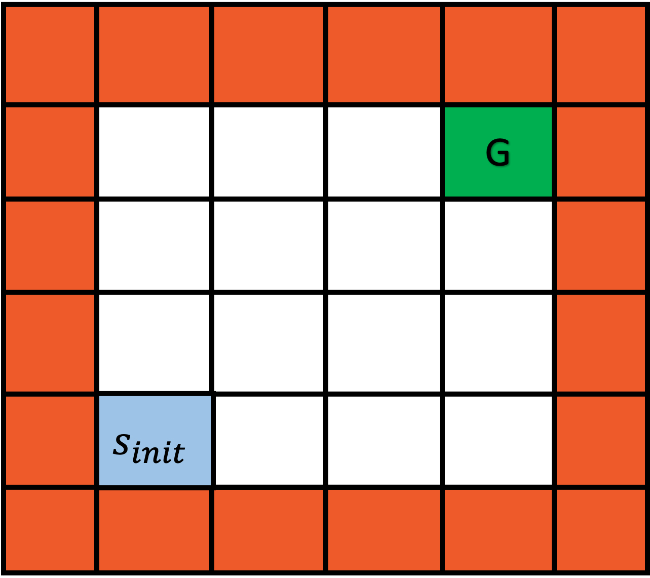
In this section, we evaluate an implementation of our algorithm. All of the experiments were performed on a laptop with core i7 CPU at 3.10GHz, with 8GB of RAM. We considered a reach-avoid controller synthesis problem in the gridworld example described in Fig. 1. The world is characterized by the number of cells per column and row, which is denoted by $l\in\mathbb{N}^{\geq 4}$. The agent can move using the cardinal directions, i.e., $A=\set{\mathit{right},\mathit{left},\mathit{up},\mathit{down}}$. Movement along an intended direction succeeds with probability $0.9$ and fails with probability $0.1$. In case of failure, the agent does not move. Walls are considered to be absorbing, i.e., the agent will not be able to move after hitting a wall. We have conducted experiments to (1) evaluate the empirical performance of our algorithcm, (2) observe how episode length vary throughout the run of our algorithm, and (3) assess the sample complexity of our method.

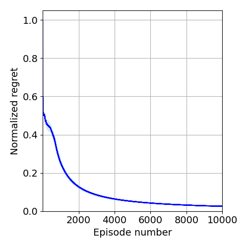
Empirical performance. Fig. 2 illustrates the variations of empirical mean for the normalized regret $R(K)/K$ for our regret-free algorithm which is run for the gridworld example with $l=6$. We set $\delta=0.1$ over $10$ runs. Furthermore, we group all of the cells associated with the wall into an absorbing state $B$, such that we have $|S|=17$ and $|A|=4$. The target specification is $\varphi=\neg B\mathbin{\sf U}G$. It can be observed that the empirical mean of regret drops very quickly, which implies that the algorithm successfully finds an optimal policy within the few first episodes.

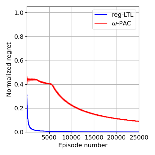
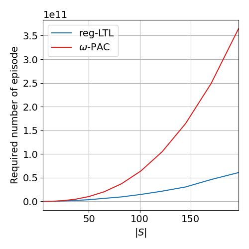
We also compare the performance of our proposed method with the $\omega$-PAC algorithm proposed in (Perez et al., 2023), which is the only existing method that supports guaranteed controller synthesis against infinite-horizon temporal specifications. The $\omega$-PAC algorithm takes a confidence parameter $\delta\in(0,1)$ and a precision parameter $\varepsilon\in(0,1)$ and provides a policy which has $\varepsilon$-optimal satisfaction probability with confidence $1-\delta$. Fig. 3 illustrates that our proposed algorithm converges much faster. We believe that this is because our algorithm uses the intermediate confidence bounds, while the $\omega$-PAC algorithm waits until enough many samples are collected, and only then updates its policy.

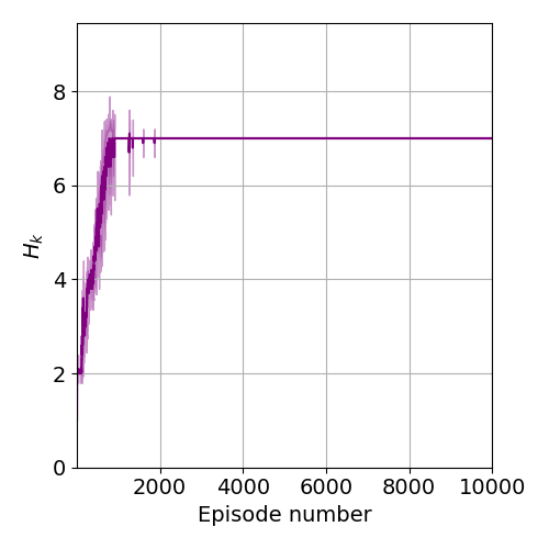
Episode length variations. Fig. 4 illustrates the variations in $H_{k}$ for different episodes. Initially, our algorithm assigns very small values to $H_{k}$, because the expected time to reach $G$ in the optimistic MDP is small. As the empirical transition probabilities become more precise, the estimation over the expected time to reach $G$ takes more accurate values.

Sample complexity. Although our method and $\omega$-PAC algorithm provide different guarantees, we relate them through definition of a related complexity metric. The sample complexity of the $\omega$-PAC algorithm is characterized with $C$ that is the number of learning episodes with non-$\varepsilon$-optimal satisfaction probability.We define $k^{\ast}_{reg}(\delta,\varepsilon)$ as the smallest number of episodes $k$ for which our regret-free algorithm with confidence $1-\delta$ satisfies $\frac{R(k)}{k}\leq\varepsilon$. Furthermore, we define $k^{\ast}_{PAC}(\delta,\varepsilon)$ as the minimum number of episodes after which with confidence $1-\delta$ the $\omega$-PAC algorithm satisfies $\frac{\mathcal{C}_{k}}{k}\leq\varepsilon$. Fig. 5 illustrates the variations of $k^{\ast}_{reg}(0.1,0.1)$ and $k^{\ast}_{PAC}(0.1,0.1)$ for gridworld examples with $4\leq l\leq 16$. Note that changes in $l$ influences size of state space ($|S|=(l-2)^{2}+1$), optimal policy’s average time for hitting the goal ($\Gamma=2(l-3)+1$) and also the (minimum) $\varepsilon$-recurrence time $T=(l-2)^{2}+1$. It can be observed that our algorithm provides a tighter bound specially for the larger examples.

Refer to caption
Figure 5: Comparison of the theoretical sample complexities for our proposed algorithm and the $\omega$-PAC algorithm (Perez et al., 2023), when applied to the gridworld example with various sizes ($4\leq l\leq 16$).

7 Discussion and Conclusions

In this paper, we proposed a regret-free algorithm for the control synthesis problem over MDPs against infinite-horizon LTL specifications. The defined regret quantifies the accumulated deviation over the probability of satisfying the given LTL specification. Below, we have discussed several aspects of the proposed scheme.

Possibility of applying the regret-free algorithms that are proposed for SSP. The assumptions that are needed for solving SSP in a regret free way, are inherently non-applicable to our target setting as we discussed in the related work section. In particular, relaxing the requirement for existence of a proper policy (which is equivalent to the existence of a policy which satisfies the given LTL specification with probability one) requires attributing a large enough cost to the policies which may end up visiting the non-accepting MECs. Such an assumption (even in the case finding such an upper bound is feasible) would automatically require defining a cost structure over the product MDP which would in turn change the function of regret so that it can only be defined with respect to the accumulated cost and not the probability of satisfying the given specification. However, we desire knowing the value of regret with respect to the satisfaction probability and not any artificially defined accumulated cost.

Possibility of applying UCRL2 algorithm. UCRL2 is a useful regret-free algorithm which is proposed for communicating MDPs with bounded diameter. Our setting is not appropriate for applying UCRL2 as the product MDP would not be communicating after all. However, it may be noticed that our second assumption, i.e., the knowledge over an upper bound for the expected hitting time of the optimal policy is a weaker assumption with respect to the main assumption for UCRL2 that is the knowledge over the diameter of the underlying MDP.

References

  • Agarwal et al. (2014) Agarwal, A., Hsu, D., Kale, S., Langford, J., Li, L., and Schapire, R. Taming the monster: A fast and simple algorithm for contextual bandits. In Xing, E. P. and Jebara, T. (eds.), Proceedings of the 31st International Conference on Machine Learning, volume 32 of Proceedings of Machine Learning Research, pp.  1638–1646, Bejing, China, 22–24 Jun 2014. PMLR. URL https://proceedings.mlr.press/v32/agarwalb14.html.
  • Alur et al. (2022) Alur, R., Bansal, S., Bastani, O., and Jothimurugan, K. A framework for transforming specifications in reinforcement learning. In Principles of Systems Design: Essays Dedicated to Thomas A. Henzinger on the Occasion of His 60th Birthday, pp.  604–624. Springer, 2022.
  • Auer & Ortner (2007) Auer, P. and Ortner, R. Logarithmic Online Regret Bounds for Undiscounted Reinforcement Learning, pp.  49–56. The MIT Press, September 2007. ISBN 9780262256919. doi: 10.7551/mitpress/7503.003.0011. URL http://dx.doi.org/10.7551/mitpress/7503.003.0011.
  • Auer et al. (2008) Auer, P., Jaksch, T., and Ortner, R. Near-optimal regret bounds for reinforcement learning. Advances in neural information processing systems, 21, 2008.
  • Baier & Katoen (2008) Baier, C. and Katoen, J.-P. Principles of model checking. MIT press, 2008.
  • Bozkurt et al. (2021) Bozkurt, A. K., Wang, Y., Zavlanos, M. M., and Pajic, M. Model-free reinforcement learning for stochastic games with linear temporal logic objectives. In 2021 IEEE International Conference on Robotics and Automation (ICRA), pp.  10649–10655. IEEE Press, 2021. doi: 10.1109/ICRA48506.2021.9561989. URL https://doi.org/10.1109/ICRA48506.2021.9561989.
  • Cai et al. (2020) Cai, M., Xiao, S., Li, B., Li, Z., and Kan, Z. Reinforcement learning based temporal logic control with maximum probabilistic satisfaction. CoRR, abs/2010.06797, 2020. URL https://arxiv.org/abs/2010.06797.
  • Camacho et al. (2019) Camacho, A., Icarte, R. T., Klassen, T. Q., Valenzano, R. A., and McIlraith, S. A. Ltl and beyond: Formal languages for reward function specification in reinforcement learning. In International Joint Conference on Artificial Intelligence, 2019.
  • Dann et al. (2017) Dann, C., Lattimore, T., and Brunskill, E. Unifying pac and regret: uniform pac bounds for episodic reinforcement learning. In Proceedings of the 31st International Conference on Neural Information Processing Systems, NIPS’17, pp.  5717–5727, Red Hook, NY, USA, 2017. Curran Associates Inc. ISBN 9781510860964.
  • Fruit et al. (2018) Fruit, R., Pirotta, M., and Lazaric, A. Near optimal exploration-exploitation in non-communicating markov decision processes. In Proceedings of the 32nd International Conference on Neural Information Processing Systems, NIPS’18, pp.  2998–3008, Red Hook, NY, USA, 2018. Curran Associates Inc.
  • Fu & Topcu (2014) Fu, J. and Topcu, U. Probably approximately correct MDP learning and control with temporal logic constraints. In Robotics: Science and Systems X, University of California, Berkeley, USA, July 12-16, 2014, 2014.
  • Hahn et al. (2019) Hahn, E. M., Perez, M., Schewe, S., Somenzi, F., Trivedi, A., and Wojtczak, D. Omega-regular objectives in model-free reinforcement learning. In Tools and Algorithms for the Construction and Analysis of Systems: 25th International Conference, TACAS 2019, Held as Part of the European Joint Conferences on Theory and Practice of Software, ETAPS 2019, Prague, Czech Republic, April 6–11, 2019, Proceedings, Part I, pp. 395–412, Berlin, Heidelberg, 2019. Springer-Verlag. ISBN 978-3-030-17461-3. doi: 10.1007/978-3-030-17462-0˙27. URL https://doi.org/10.1007/978-3-030-17462-0_27.
  • Hasanbeig et al. (2019) Hasanbeig, M., Kantaros, Y., Abate, A., Kroening, D., Pappas, G. J., and Lee, I. Reinforcement learning for temporal logic control synthesis with probabilistic satisfaction guarantees. In 2019 IEEE 58th Conference on Decision and Control (CDC), pp.  5338–5343. IEEE Press, 2019. doi: 10.1109/CDC40024.2019.9028919. URL https://doi.org/10.1109/CDC40024.2019.9028919.
  • Icarte et al. (2018) Icarte, R. T., Klassen, T. Q., Valenzano, R. A., and McIlraith, S. A. Using reward machines for high-level task specification and decomposition in reinforcement learning. In International Conference on Machine Learning, 2018.
  • Kazemi et al. (2022) Kazemi, M., Perez, M., Somenzi, F., Soudjani, S., Trivedi, A., and Velasquez, A. Translating omega-regular specifications to average objectives for model-free reinforcement learning. In Proceedings of the 21st International Conference on Autonomous Agents and Multiagent Systems, AAMAS ’22, pp.  732–741, Richland, SC, 2022. International Foundation for Autonomous Agents and Multiagent Systems. ISBN 9781450392136.
  • Kearns & Singh (2002) Kearns, M. and Singh, S. Near-optimal reinforcement learning in polynomial time. Machine Learning, 49:209–232, 2002. URL https://api.semanticscholar.org/CorpusID:2695116.
  • Latouche & Ramaswami (1999) Latouche, G. and Ramaswami, V. Introduction to Matrix Analytic Methods in Stochastic Modeling. Society for Industrial and Applied Mathematics, 1999. doi: 10.1137/1.9780898719734. URL https://epubs.siam.org/doi/abs/10.1137/1.9780898719734.
  • Oura et al. (2020) Oura, R., Sakakibara, A., and Ushio, T. Reinforcement learning of control policy for linear temporal logic specifications using limit-deterministic generalized büchi automata. IEEE Control Systems Letters, 4(3):761–766, July 2020. ISSN 2475-1456. doi: 10.1109/lcsys.2020.2980552. URL http://dx.doi.org/10.1109/LCSYS.2020.2980552.
  • Perez et al. (2023) Perez, M., Somenzi, F., and Trivedi, A. A PAC learning algorithm for LTL and omega-regular objectives in mdps. CoRR, abs/2310.12248, 2023. doi: 10.48550/ARXIV.2310.12248. URL https://doi.org/10.48550/arXiv.2310.12248.
  • Rosenberg et al. (2020) Rosenberg, A., Cohen, A., Mansour, Y., and Kaplan, H. Near-optimal regret bounds for stochastic shortest path. In International Conference on Machine Learning, pp. 8210–8219. PMLR, 2020.
  • Sickert et al. (2016) Sickert, S., Esparza, J., Jaax, S., and Křetínský, J. Limit-deterministic büchi automata for linear temporal logic. In Chaudhuri, S. and Farzan, A. (eds.), Computer Aided Verification, pp.  312–332, Cham, 2016. Springer International Publishing. ISBN 978-3-319-41540-6.
  • Srinivas et al. (2012) Srinivas, N., Krause, A., Kakade, S. M., and Seeger, M. W. Information-theoretic regret bounds for gaussian process optimization in the bandit setting. IEEE Transactions on Information Theory, 58(5):3250–3265, 2012. doi: 10.1109/TIT.2011.2182033.
  • Tarbouriech et al. (2020) Tarbouriech, J., Garcelon, E., Valko, M., Pirotta, M., and Lazaric, A. No-regret exploration in goal-oriented reinforcement learning. In III, H. D. and Singh, A. (eds.), Proceedings of the 37th International Conference on Machine Learning, volume 119 of Proceedings of Machine Learning Research, pp.  9428–9437. PMLR, 13–18 Jul 2020. URL https://proceedings.mlr.press/v119/tarbouriech20a.html.
  • Voloshin et al. (2022) Voloshin, C., Le, H. M., Chaudhuri, S., and Yue, Y. Policy optimization with linear temporal logic constraints. In Advances in Neural Information Processing Systems 35: Annual Conference on Neural Information Processing Systems 2022, NeurIPS 2022, New Orleans, LA, USA, November 28 - December 9, 2022, 2022.
  • Yang et al. (2021) Yang, C., Littman, M., and Carbin, M. On the (in) tractability of reinforcement learning for ltl objectives. arXiv preprint arXiv:2111.12679, 2021.
Algorithm 5 Proposed algorithm for learning graphs
  Input: Initial state $s_{\mathsf{init}}$, minimum transition probability $p_{min}^{(t)}$,state and action sets $S$ and $A$.
  Compute $n^{\ast}$, that is minimum number of samples required to determine all outgoing transitions for any state-action pair $(s,a)\in S\times A$ with confidence $1-\delta_{1}$, assuming minimum transition probability $p_{min}$,
  $E\leftarrow\emptyset$
  $t\leftarrow 0$
  for $s\in S\setminus s_{\mathsf{init}}$ do
     Compute a policy $\pi^{(s)}$ under which $s$ is reachable from $s_{\mathsf{init}}$
     for $a\in A$ do
        $n\leftarrow\#\{t^{\prime}<t\colon s_{t}=s,a_{t}=a\}$
        while $n<n^{\ast}$ do
           $s_{t}\leftarrow s_{\mathsf{init}}$
           Run the transition from state-action pair $(s_{t},\pi^{(s)}(s_{t}))$ and observe $s_{t+1}$
           if $s_{t}=s$ then
              $n\leftarrow n+1$
              break
           end if
           tt+1𝑡𝑡1t\leftarrow t+1
        end while
     end for
  end for

Appendix A Graph Identification

In order to propose a regret-free controller synthesis method, we need to know the underlying MECs. In this section, we show how to use the knowledge of minimum transition probability $p_{min}\in\mathbb{R}^{>0}$ of a given MDP $\mathcal{M}$ in order to identify the underlying graph of the MDP which is valid with a desired confidence. By the following lemma, we can determine the number of samples needed in order to ensure whether a transition exists or not.

Lemma A.1.

(Voloshin et al., 2022) For any state-action pair $(s,a)\in S\times A$, let $\hat{T}_{n}(s^{\prime}\mid s,a)$ denote the empirical transition probability estimation for the transition probability $T(s^{\prime}\mid s,a)$ after sampling $(s,a)$ for $n$ times. Given a positive lower bound over the minimum transition probability $p_{min}\in(0,1)$ and a confidence parameter $\delta\in(0,1)$, we have $(s,a,s^{\prime})\notin E$ with confidence $1-\delta$ if $\hat{T}_{n^{\ast}}(s^{\prime}\mid s,a)=0$, for

$$n^{\ast}>\psi^{-1}(p_{min})$$ (20)

, where

$$\psi(n)=\sqrt{\frac{1}{2}\zeta(n)}+\frac{7}{3}\zeta(n),$$ (21)

and $\zeta(n)=\frac{\log(4n^{2}|S|^{2}|A|p_{min})}{(n-1)}$ if $n\geq 1$.

Remark A.2.

To compute policies $\pi^{(s)}$ for $s\in S$, one needs to use undiscounted RL formulations which explicitly can handle the exploration-exploitation trade-off. $E^{3}$ (Kearns & Singh, 2002) and $\omega$-PAC (Perez et al., 2023) are two such approaches which use $\varepsilon$-return mixing time and $\varepsilon$-recurrence time, respectively, in order to avoid unbounded explorations. In our case, we could define an $\varepsilon$-covering time for a policy $\pi^{(s)}$, as the number of time steps required to visit $s$ for $n^{\ast}$ times with probability at least $1-\varepsilon$ for $\varepsilon\in(0,1)$. Similar to the theoretical guranatees of methods like $E^{3}$, we could easilly see that our graph learning algorithm has a sample complexity that is polynomial in the size of state and action spaces and maximum $\varepsilon$-covering time among all policies.

Alg. 5 outlines our proposed algorithm to learn the graph of a given MDP. There are two main steps: (1) for every state $s\in S$, we utilize an RL algorithm to get a policy $\pi^{(s)}$ under which, $s$ is reachable from $s_{\mathsf{init}}$ (with positive probability); (2) we run $\pi^{(s)}$ for every $a\in A$ until $(s,a)$ is visited for $n^{\ast}$ times; upon reaching $(s,a)$, we collect the resulted outgoing transition by running the MDP. Within the rest of this paper, we are going to use the MDP graph $\chi_{\mathcal{M}}$ which is correct with confidence $1-\delta$.

Appendix B Proofs

B.1 Proof of Lem. 4.2

Proof.

Assuming that $\lambda^{\ast}$ is finite implies that there exists at least one policy under which $G$ is reachable from $s_{\mathsf{init}}$. Under such a policy, in the worst-case scenario, each state in the Markov chain must be visited at least once. Visiting every state requires following a path of length $|S|$, which occurs with probability $p_{min}^{|S|}$. After $l$ attempts of traversing this path, the probability of success at least once is given by $1-(1-p_{min}^{|S|})^{l}$. If $l\geq\frac{\log(\delta)}{\log(1-p_{min}^{|S|})}$, then $1-(1-p_{min}^{|S|})^{l}\geq 1-\delta$. Finally, since each of the $l$ attempts takes $|S|$ steps in the worst case, the total number of steps is bounded by $\Lambda\leq|S|l=|S|\frac{\log(\delta)}{\log(1-p_{min}^{|S|})}$.

B.2 Proof of Lem. 4.5

Proof.

First, using the Markov’s inequality (since $x\mapsto x^{r}$ is a non-decreasing mapping for non-negative reals), we have

$$\mathbb{P}(\tilde{\lambda}_{k}(s)\geq H_{k}-1)\leq\frac{\mathbb{E}[\tilde{\lambda}_{k}(s)^{r}]}{(H_{k}-1)^{r}}.$$

Now, we note that by Lem. 15 in (Tarbouriech et al., 2020), we have if $\tilde{\lambda}_{k}(s)\leq\lambda$ for every $s\in S\setminus(G\cup B)$ and $\lambda\geq 2$, then

$$\mathbb{E}(\tilde{\lambda}_{k}(s)^{r})\leq 2(r\lambda)^{r},$$

for any $r\geq 1$. Therefore, substituting $\lambda$ with $\Lambda$, we will have

$$\mathbb{P}(\tilde{\lambda}_{k}(s)\geq H_{k}-1)\leq\frac{2(r\Lambda)^{r}}{(H_{k}-1)^{r}},$$ (22)

Note that there exists $y\in S$ such that

$\displaystyle\|\tilde{Q}^{H_{k}-2}\|_{\infty}$ $\displaystyle=\mathbf{1}_{y}^{\top}\tilde{Q}^{H_{k}-2}\mathbf{1}=\mathbb{P}(\tilde{\lambda}_{k}(y)>H_{k}-2)$
$\displaystyle\qquad=\mathbb{P}(\tilde{\lambda}_{k}(y)\geq H_{k}-2).$ (23)

By definition of $H_{k}$ we have $\|\tilde{Q}^{H_{k}-2}\|_{\infty}>1/\sqrt{k}$. Combining this with Eqs. (22), (B.2) yields

$$\frac{2(r\Lambda)^{r}}{(H_{k}-1)^{r}}>1/\sqrt{k},$$

which implies that

$$H_{k}-1<r\Lambda(2\sqrt{k})^{1/r}.$$

By selecting $r=\Big{\lceil}log(2\sqrt{k})\Big{\rceil}$, we get

$$H_{k}-1<\lceil log(2\sqrt{k})\rceil\Lambda(2\sqrt{k})^{\frac{1}{\Big{\lceil}log(2\sqrt{k})\Big{\rceil}}}\leq\Big{\lceil}3\Lambda log(2\sqrt{k})\Big{\rceil}.$$

Hence

$$\alpha_{K}\leq\Big{\lceil}3\Lambda log(2\sqrt{K})\Big{\rceil}.$$

In order to prove the sub linear regret bound, we make use of the Azuma-Hoeffding inequality.

Lemma B.1 (Azuma-Hoeffding inequality, Hoeffding 1963).

Let $X_{1},X_{2},\dots$ be a martingale difference sequence with $|X_{l}|\leq c$ for all $l$. Then for all $\gamma>0$ and $n\in N$,

$$\mathbb{P}\{\sum_{l=1}^{n}X_{l}\geq\gamma\}\leq exp(-\frac{\gamma^{2}}{2nc^{2}}).$$

Now, we proceed by showing why k=1KΔk(f,1)superscriptsubscript𝑘1𝐾superscriptsubscriptΔ𝑘𝑓1\sum_{k=1}^{K}\Delta_{k}^{(f,1)} grows sub linearly with K𝐾K.

B.3 Proof of Lem. 4.6

Proof.

In order to reformulate the regret, we define the following reward function $r\colon S\rightarrow\{0,1\}$

$$r(s)=\begin{cases}0&s\notin G\\ 1&s\in G\end{cases}.$$ (24)

Further, for the time step $h$ within episode $k$ we define

$$\Theta_{k,h}(s_{k,h})\coloneqq\tilde{v}_{k}(s_{k,h})-\sum_{t=h}^{H_{k,\mathcal{I}_{k}(h)}-1}r(s_{k,t})$$

where $\mathcal{I}_{k}\colon[1;H_{k}]\rightarrow[1;I_{k}]$ maps the time points in episode $k$ into the corresponding interval, and $H_{k,i}$ denotes the length of the $i^{th}$ interval within the $k^{th}$ episode for $1\leq i\leq I_{k}$ and $H_{k,0}=1$. Therefore, we have

$$\sum_{k=1}^{K}\Delta_{k}^{(1)}=\sum_{k=1}^{K}\sum_{i=1}^{I_{k}}\Theta_{k,H_{k,i-1}}(s_{k,H_{k,i-1}}).$$

Let us further define

$$\Phi_{k,h}\coloneqq\tilde{v}_{k}(s_{k,h+1})-\sum_{y\in S}p(y\mid s_{k,h},\tilde{\pi}_{k}(s_{k,h}))\tilde{v}_{k}(y),$$ (25)

where $p(\cdot\mid\cdot,\cdot)$ corresponds to the transition probability in the true MDP $\mathcal{M}_{\varphi}$. Similarly, we denote by $\tilde{p}_{k}(\cdot\mid\cdot,\cdot)$ for the transition probability in the optimistic MDP $\tilde{\mathcal{M}}_{k}$. Note that for $s_{k,h}\in G\cup B$, we have $\Theta_{k,h}(s_{k,h})=0$. For $s_{k,h}\notin G\cup B$, we have

$\displaystyle\Theta_{k,h}(s_{k,h})=\tilde{v}_{k}(s_{k,h})-\sum_{t=h}^{H_{k,\mathcal{I}_{k}(h)}-1}r(s_{k,t})$
$\displaystyle\leq\tilde{\mathcal{L}}_{k}\tilde{v}_{k}(s_{k,h})+\varepsilon_{k}-\sum_{t=h}^{H_{k,\mathcal{I}_{k}(h)}-1}r(s_{k,t})$
$\displaystyle=\sum_{y\in S}\tilde{p}_{k}(y\mid s_{k,h},\tilde{\pi}_{k}(s_{k,h}))\tilde{v}_{k}(y)$
$\displaystyle\qquad+\varepsilon_{k}-r(s_{k,h})-\sum_{t=h+1}^{H_{k,\mathcal{I}_{k}(h)}-1}r(s_{k,t})$
$\displaystyle=\sum_{y\in S}(\tilde{p}_{k}(y\mid s_{k,h},\tilde{\pi}_{k}(s_{k,h}))$
$\displaystyle\qquad-p(y\mid s_{k,h},\tilde{\pi}_{k}(s_{k,h})))\tilde{v}_{k}(y)$
$\displaystyle\qquad+\sum_{y\in S}p(y\mid s_{k,h},\tilde{\pi}_{k}(s_{k,h}))\tilde{v}_{k}(y)+\varepsilon_{k}-\sum_{t=h+1}^{H_{k,\mathcal{I}_{k}(h)}-1}r(s_{k,t})$
$\displaystyle\leq 2\beta_{k}(s_{k,h},\tilde{\pi}_{k}(s_{k,h}))\times 1$
$\displaystyle\qquad+(\sum_{y\in S}p(y\mid s_{k,h},\tilde{\pi}_{k}(s_{k,h}))\tilde{v}_{k}(y)-\tilde{v}_{k}(s_{k,h+1}))$
$\displaystyle\qquad+\varepsilon_{k}+(\tilde{v}_{k}(s_{k,h+1})-\sum_{t=h+1}^{H_{k,\mathcal{I}_{k}(h)}-1}r(s_{k,t}))$
$\displaystyle\leq 2\beta_{k}(s_{k,h},\tilde{\pi}_{k}(s_{k,h}))+\Phi_{k,h}+\varepsilon_{k}+\Theta_{k,h+1}(s_{k,h+1}),$

where we used Eq. (6) for the first inequality, the fact that $r(s_{k,t})=0$ for every $s_{k,t}\notin G\cup B$ for the second equality, $\tilde{v}_{k}(y)\leq 1$ for every $y\in S$ for the third equality, definition of $\beta_{k}$ (Eq. (4)) for the second inequality, and definition of $\Phi_{k,h}$ (Eq. (25)) for the last inequality. Also, note that By telescopic sum we get

$\displaystyle\Theta_{k,H_{k,i}}(s_{k,H_{k,i}})$ $\displaystyle=\sum_{h=H_{k,i}}^{H_{k,i+1}-2}(\Theta_{k,h}(s_{k,h})-\Theta_{k,h+1}(s_{k,h+1}))$
$\displaystyle\qquad+\Theta_{k,H_{k,i+1}-1}(s_{k,H_{k,i+1}-1})$
$\displaystyle\leq\sum_{h=1}^{H_{k,i+1}-2}(2\beta_{k}(s_{k,h},\tilde{\pi}_{k}(s_{k,h}))+\Phi_{k,h}+\varepsilon_{k})$
$\displaystyle\qquad+\Theta_{k,H_{k,i+1}-1}(s_{k,H_{k,i+1}-1})$
$\displaystyle\leq\sum_{h=1}^{H_{k,i+1}-2}2\beta_{k}(s_{k,h},\tilde{\pi}_{k}(s_{k,h}))$
$\displaystyle\qquad+\sum_{h=1}^{H_{k,i+1}-2}\Phi_{k,h}+H_{k,i+1}\varepsilon_{k}$

where we used the arguments we made in the previous step of the proof to establish the first inequality, the fact that $\Theta_{k,H_{k,i+1}-1}(s_{k,H_{k,i+1}-1})=0$ by definition as $s_{k,t_{k,i+1}-1}\in G\cup B$ for every $1\leq i\leq I_{k}$ for the last inequality . By summing over all of the episodes we have

$\displaystyle\sum_{k=1}^{K}\sum_{i=1}^{I_{k}}\Theta_{k,H_{k,i-1}}(s_{k,H_{k,i-1}})$
$\displaystyle\leq\sum_{k=1}^{K}\sum_{i=1}^{I_{k}}\sum_{h=H_{k,i-1}}^{H_{k,i}-1}\Phi_{k,h}$
$\displaystyle\qquad+2\sum_{k=1}^{K}\sum_{i=1}^{I_{k}}\sum_{h=H_{k,i-1}}^{H_{k,i}-1}\beta_{k}(s_{k,h},\tilde{\pi}_{k}(s_{k,h}))$
$\displaystyle\qquad+\sum_{k=1}^{K}H_{k}\varepsilon_{k}.$ (26)

In order to bound the first term, we note that

$\displaystyle\sum_{k=1}^{K}\sum_{i=1}^{I_{k}}\sum_{h=H_{k,i-1}}^{H_{k,i}-1}\Phi_{k,h}=\sum_{k=1}^{K}\sum_{h=t_{k}}^{t_{k+1}-1}\Phi_{k,h}$

Therefore, we can write

$\displaystyle\mathbb{P}\left(\sum_{k=1}^{K}\sum_{h=t_{k}}^{t_{k+1}-1}\Phi_{k,h}\geq 2\sqrt{2(\sum_{k=1}^{K}H_{k})log(\frac{2(\sum_{k=1}^{K}H_{k})^{2}}{\delta})}\right)$
$\displaystyle\leq\mathbb{P}\left(\sum_{k=1}^{K}\sum_{h=t_{k}}^{t_{k+1}-1}\Phi_{k,h}\geq 2\sqrt{2nlog(\frac{2n^{2}}{\delta})}\cap\sum_{k=1}^{K}H_{k}=n\right).$

Let $\mathcal{G}_{q}$ denote the history of all random events up to (and including) step $h$ of episode $k$, i.e., $q=\sum_{k^{\prime}=1}^{k-1}H_{k^{\prime}}+h$. We have $\mathbb{E}(\Phi_{k,h}\mid\mathcal{G}_{q})=0$, and furthermore $H_{k}$ is selected at the beginning of episode $k$, and so it is adapted with respect to $\mathcal{G}_{q}$. Hence $\Phi_{k,h}$ is a martingale difference with $|\Phi_{k,h}|\leq 1$. Therefore, by Azuma-Hoeffding’s inequality, we have with probability $1-\frac{2\delta}{3}$

$$\mathbb{P}\left(\sum_{k=1}^{K}\sum_{h=t_{k}}^{t_{k+1}-1}\Phi_{k,h}\geq 2\sqrt{2(\sum_{k=1}^{K}H_{k})log(\frac{3(\sum_{k=1}^{K}H_{k})^{2}}{\delta})}\right).$$

Now, we proceed to bound the second term in Eq. B.3. Let $N^{(1)}$ denote the number of samples only collected during attempts in phase (1) and $N^{(1)+}=\max\{1,N^{(1)}\}$. Also let $T_{K,1}$ denote the number of time steps taken within the episodes which end before the deadline $H_{k}$. We can write

$\displaystyle\sum_{k=1}^{K}\sum_{h=1}^{H_{k}-1}\sqrt{\frac{1}{N_{k}^{(1)}(s_{k,h},\tilde{\pi}_{k}(s_{k,h}))}}\leq\sum_{s,a}\sum_{n=1}^{N_{K}^{(1)}}\sqrt{\frac{1}{n}}$
$\displaystyle\qquad\leq 2\sqrt{|S||A|}\sqrt{\sum_{s,a}N_{K}^{(1)}(s,a)}\leq 2\sqrt{|S||A|T_{K,1}}.$

Now, first note that by Lem. 4 in (Tarbouriech et al., 2020) we have that mappings $\sqrt{\frac{\log(cx)}{x}}$ is a non-increasing function for $c\geq 4$ and $x\geq 1$. Also noting that $N_{k}^{+}(s,a)\geq N_{k}^{(1)+}(s,a)$, we get for $|A|\geq 2$ that

$\displaystyle\beta_{k}(s,a)$ $\displaystyle=\sqrt{\frac{8|S|\log(2|A|N_{k}^{+}/\delta)}{\max{(1,N_{k}^{+}(s,a))}}}$
$\displaystyle\leq\sqrt{\frac{8|S|\log(2|A|N_{k}^{(1)+}(s,a)/\delta)}{\max{(1,N_{k}^{(1)+}(s,a))}}}.$

Therefore, we obtain

$$\sum_{k=1}^{K}\sum_{h=1}^{H_{k}-1}\beta_{k}(s_{k,h},\tilde{\pi}_{k}(s_{k,h}))\leq 2|S|\sqrt{8|A|T_{K,1}\log(\frac{2|A|T_{k,1}}{\delta})}.$$

Finally, we bound the last term in Eq. (B.3).

$$\sum_{k=1}^{K}H_{k}\varepsilon_{k}\leq\sum_{t=1}^{T_{K,1}}\frac{\alpha_{K}}{2t}\leq\alpha_{K}\frac{1+\log(K\alpha_{K})}{2},$$

where $\alpha_{K}=\max_{1\leq k\leq K}H_{k}$. Putting everything together yields that inequality (4.6) holds with probability at least $1-\delta$. ∎

B.4 Proof of Lem. 4.7

Proof.

We define $X_{k,i}\coloneqq v_{k}(s_{\mathsf{init}})-v_{k,i}(s_{\mathsf{init}})$. Note that $\mathbb{E}(X_{k,i})=0$ and $|X_{k,i}|\leq 1$ for every $1\leq k\leq K$ and $1\leq i\leq I_{k}$. We have

$$\Delta_{k}^{(f,2)}=\sum_{i=1}^{I_{k}}v_{k}(s_{\mathsf{init}})-v_{k,i}(s_{\mathsf{init}})=\sum_{i=1}^{I_{k}}X_{k,i}.$$

Therefore by application of the Azuma-Hoeffding lemma and using the fact that $K\alpha_{k}\geq\sum_{k=1}^{K}I_{k}$ we get

$\displaystyle\mathbb{P}\{\sum_{k=1}^{K}\Delta_{k}^{(f,2)}$ $\displaystyle\geq\sqrt{2K\alpha_{K}\log\frac{1}{\delta}}\}$
$\displaystyle\leq\exp(-\frac{2K\alpha_{K}\log\frac{1}{\delta}}{2\sum_{k=1}^{K}I_{k}})$
$\displaystyle\leq\exp(-\log\frac{1}{\delta})=\delta.$

In Lemma 4.5, we have already shown that $\alpha_{K}$ grows logarithmically with $K$ which proves that $\sum_{k=1}^{K}\Delta_{k}^{(f,2)}$ grows sub linearly with $K$.

Let $F_{K}$ denote the number of episodes in which $G$ is not reached within the phase (1). By using arguments similar to the ones stated in Lem. 7 of (Tarbouriech et al., 2020), we can state that with high probability $F_{K}$ grows sublinearly.

B.5 Proof of Lem. 4.8

Proof.

Let $\tau_{k}$ and $\tilde{\lambda}_{k}$ denote the hitting times of policy $\tilde{\pi}_{k}$ in the true and optimistic models, respectively. We define

$$\Gamma_{k,h}(s_{k,h})=\mathbf{1}_{\tau_{k}(s_{k,h})>H_{k}-h}-\mathbb{P}(\tilde{\lambda}_{k}((s_{k,h}))>H_{k}-h).$$

Note that we have

$\displaystyle F_{K}$ $\displaystyle=\sum_{k=1}^{K}\mathbf{1}_{\tau_{k}(s_{k,1})>H_{k}-1}$
$\displaystyle=\sum_{k=1}^{K}\Gamma_{k,1}(s_{k,1})+\sum_{k=1}^{K}\mathbb{P}(\tilde{\lambda}_{k}(s_{\mathsf{init}})>H_{k}-1).$

Let

$$\tilde{P}_{k}^{\prime}=\begin{bmatrix}\tilde{Q}_{k}&\vdots&\tilde{\boldsymbol{\beta}}_{k}\\ \dots&\dots&\dots\\ g&\vdots&0\end{bmatrix},$$

denote the transition probability matrix of the DTMC created by connecting $B$ to $s_{\mathsf{init}}$. Let $\tilde{p}_{k}^{\prime}(\cdot\mid\cdot,\cdot)$ denote the transition probability in the optimistic model $\tilde{\mathcal{M}}_{k}^{\prime}$ (that is the optimistic MDP constructed from $\tilde{\mathcal{M}}_{k}$ by connecting states in $B$ into $s_{\mathsf{init}}$). Similarly, let $p^{\prime}(\cdot\mid\cdot,\cdot)$ denote the transition probability in the MDP $\mathcal{M}_{p}^{\prime}$ (that is the MDP constructed from $\mathcal{M}_{p}$ by connecting states in $B$ into $s_{\mathsf{init}}$). Since for $1\leq h\leq H_{k}-1$, $\mathbf{1}_{\tau_{k}(s_{k,h})>H_{k}-h}=\mathbf{1}_{\tau_{k}(s_{k,h+1})>H_{k}-h-1}$ we have

$\displaystyle\Gamma_{k,h}(s_{k,h})=\mathbf{1}_{\tau_{k}(s_{k,h+1})>H_{k}-h-1}$
$\displaystyle\qquad-\sum_{y\in S}\tilde{p}_{k}^{\prime}(y\mid s_{k,h},\tilde{\pi}_{k}(s_{k,h}))\mathbb{P}(\tilde{\lambda}_{k}(y)>H_{k}-h-1)$
$\displaystyle\leq\mathbf{1}_{\tau_{k}(s_{k,h+1})>H_{k}-h-1}$
$\displaystyle-(\sum_{y\in S}\tilde{p}_{k}^{\prime}(y\mid s_{k,h},\tilde{\pi}_{k}(s_{k,h}))-p^{\prime}(y\mid s_{k,h},\tilde{\pi}_{k}(s_{k,h})))\mathbb{P}(\tilde{\lambda}_{k}(y)>H_{k}-h-1)$
$\displaystyle-\sum_{y\in S}p^{\prime}(y\mid s_{k,h},\tilde{\pi}_{k}(s_{k,h}))\mathbb{P}(\tilde{\lambda}_{k}(y)>H_{k}-h-1)$
$\displaystyle\leq\mathbf{1}_{\tau_{k}(s_{k,h+1})>H_{k}-h-1}+2\beta_{k}(s_{k,h},\tilde{\pi}_{k}(s_{k,h}))$
$\displaystyle-\sum_{y\in S}p^{\prime}(y\mid s_{k,h},\tilde{\pi}_{k}(s_{k,h}))\mathbb{P}(\tilde{\lambda}_{k}(y)>H_{k}-h-1)$
$\displaystyle=\Gamma_{k,h+1}(s_{k,h+1})+\psi_{k,h}+2\beta_{k}(s_{k,h},\tilde{\pi}_{k}(s_{k,h})),$

where we established the first inequality by adding and subtracting the term $p^{\prime}(y\mid s_{k,h},\tilde{\pi}_{k}(s_{k,h})))\mathbb{P}(\tilde{\lambda}_{k}(y)>H_{k}-h-1)$, the second inequality by using the definition of $\beta_{k}$ (Eq. (4)), and the last equality by using the following definition

$\displaystyle\psi_{k,h}$ $\displaystyle=\mathbb{P}(\tilde{\lambda}_{k}(s_{k,h+1})>H_{k}-h-1)$
$\displaystyle\qquad-\sum_{y\in S}p^{\prime}(y\mid s_{k,h},\tilde{\pi}_{k}(s_{k,h}))\mathbb{P}(\tilde{\lambda}_{k}(y)>H_{k}-h-1).$

Also, we have

$\displaystyle\Gamma_{k,H_{k}}(s_{k,H_{k}})$ $\displaystyle=\mathbf{1}_{\tau_{k}(s_{k,H_{k}})>0}-\mathbb{P}(\tilde{\lambda}_{k}(s_{k,H_{k}}>0))$
$\displaystyle=\mathbf{1}_{\tau_{k}(s_{k,H_{k}})>0}-\mathbf{1}_{\tilde{\lambda}_{k}(s_{k,H_{k}}>0)}$
$\displaystyle=\mathbf{1}_{s_{k,H_{k}}\notin G}-\mathbf{1}_{s_{k,H_{k}}\notin G}=0.$

Using the telescopic sum we get

$\displaystyle\Gamma_{k,1}(s_{k,1})$ $\displaystyle=\sum_{h=1}^{H_{k}-1}(\Gamma_{k,h}(s_{k,h})-\Gamma_{k,h+1}(s_{k,h+1}))+\Gamma_{k,H_{k}}(s_{k,H_{k}})$
$\displaystyle\leq\sum_{h=1}^{H_{k}-1}\psi_{k,h}+2\sum_{h=1}^{H_{k}-1}{\beta_{k}(s_{k,h},\tilde{\pi}_{k}(s_{k,h}))},$

where the last inequality is achieved by knowing $\Gamma_{k,H_{k}}(s_{k,H_{k}})=0$. Therefore, by summing over all episodes we get

$\displaystyle F_{K}$ $\displaystyle\leq\sum_{k=1}^{K}\sum_{h=1}^{H_{k}-1}\psi_{k,h}+2\sum_{k=1}^{K}\sum_{h=1}^{H_{k}-1}{\beta_{k}(s_{k,h},\tilde{\pi}_{k}(s_{k,h}))}$
$\displaystyle\qquad+\sum_{k=1}^{K}\mathbb{P}(\tilde{\lambda}_{k}(s_{\mathsf{init}})>H_{k}-1).$

Let $\mathcal{G}_{q}$ denote the history of all random events up to (and including) step $h$ of episode $k$, i.e., $q=\sum_{k^{\prime}=1}^{k-1}H_{k}+h$. We have $\mathbb{E}(\psi_{k,h}\mid\mathcal{G}_{q})=0$, and furthermore $H_{k}$ is selected at the beginning of episode $k$, and so it is adapted with respect to $\mathcal{G}_{q}$. Hence $\psi_{k,h}$ is a martingale difference with $|\psi_{k,h}|\leq 1$. Therefore, using similar arguments as in proof of Lem. 4.6, by Azuma-Hoeffding’s inequality, we have with probability $1-\frac{2\delta}{3}$

$\displaystyle\sum_{k=1}^{K}\sum_{h=1}^{H_{k}-1}\psi_{k,h}$ $\displaystyle\leq 2\sqrt{2(\sum_{k=1}^{K}H_{k})\log(\frac{3(\sum_{k=1}^{K}H_{k})^{2}}{\delta})}$
$\displaystyle\leq 2\sqrt{2K\alpha_{K}\log(\frac{3(K\alpha_{K})^{2}}{\delta})}.$

Further, in the same vein as proof of Lem. 4.6 we have

$\displaystyle\sum_{k=1}^{K}\sum_{h=1}^{H_{k}-1}{\beta_{k}(s_{k,h},\tilde{\pi}_{k}(s_{k,h}))}\leq 2|S|\sqrt{8|A|K\alpha_{K}\log(\frac{2|A|K\alpha_{K}}{\delta})}.$

Now, we need to bound $\sum_{k=1}^{K}\mathbb{P}(\tilde{\lambda}_{k}((s_{\mathsf{init}}))>H_{k}-1)$. Using Thm. 2.5.3 in (Latouche & Ramaswami, 1999), we have

$$\sum_{k=1}^{K}\mathbb{P}(\tilde{\lambda}_{k}(s_{\mathsf{init}})>H_{k}-1)=\sum_{k=1}^{K}\mathbf{1}_{s_{\mathsf{init}}}\tilde{Q}_{k}^{H_{k}-1}\mathbf{1},$$

where $\mathbf{1}_{s}$ denotes the $|S|-1$-sized one-hot vector at the position of state $s\in S$. Finally, from Holder’s inequality, we have

$\displaystyle\sum_{k=1}^{K}$ $\displaystyle\mathbb{P}(\tilde{\lambda}_{k}((s_{\mathsf{init}}))>H_{k}-1)=\sum_{k=1}^{K}\mathbf{1}_{s_{\mathsf{init}}}\tilde{Q}_{k}^{H_{k}-1}\mathbf{1}$
$\displaystyle\leq\sum_{k=1}^{K}\|\mathbf{1}_{s_{\mathsf{init}}}\|_{1}\|\tilde{Q}_{k}^{H_{k}-1}\mathbf{1}\|_{\infty}\leq\sum_{k=1}^{K}\|\tilde{Q}_{k}^{H_{k}-1}\mathbf{1}\|_{\infty}.$

Therefore, by the choice of $H_{k}=\min\{n>1\mid\|\tilde{Q}_{k}^{n}\|_{\infty}\leq\frac{1}{\sqrt{k}}\}$ we get

$$\sum_{k=1}^{K}\mathbb{P}(\tilde{\lambda}_{k}((s_{\mathsf{init}}))>H_{k}-1)\leq\sum_{k=1}^{K}\frac{1}{\sqrt{k}}\leq 2\sqrt{K}.$$