NeuMaDiff: Neural Material Synthesis via Hyperdiffusion

Abstract

High-quality material synthesis is essential for replicating complex surface properties to create realistic digital scenes. However, existing methods often suffer from inefficiencies in time and memory, require domain expertise, or demand extensive training data, with high-dimensional material data further constraining performance. Additionally, most approaches lack multi-modal guidance capabilities and standardized evaluation metrics, limiting control and comparability in synthesis tasks. To address these limitations, we propose NeuMaDiff, a novel neural material synthesis framework utilizing hyperdiffusion. Our method employs neural fields as a low-dimensional representation and incorporates a multi-modal conditional hyperdiffusion model to learn the distribution over material weights. This enables flexible guidance through inputs such as material type, text descriptions, or reference images, providing greater control over synthesis. To support future research, we contribute two new material datasets and introduce two BRDF distributional metrics for more rigorous evaluation. We demonstrate the effectiveness of NeuMaDiff through extensive experiments, including a novel statistics-based constrained synthesis approach, which enables the generation of materials of desired categories.

Figure 1: 3D models and scene rendered with our synthesized neural materials.

1 Introduction

Material synthesis plays a crucial role in visual computing, enabling the creation of realistic material appearances for applications in rendering, augmented reality, and scene understanding. Analytic models [42, 8, 53] are widely used to encode material appearance, due to their speed, memory efficiency, and ease of editing, which makes them suitable for real-time applications. However, their simplified representations often fail to capture the complexity of real-world materials, limiting their reconstruction accuracy. In contrast, measured data, while achieving unparalleled realism, is memory-intensive and challenging to manipulate, which restricts its flexibility. Implicit neural representations (INRs) offer a promising alternative, combining high-quality reconstructions with memory efficiency and a speed comparable with analytic models [49]. However, the lack of intuitive editing in INRs continues to hinder their usability and general adoption.

Deep-learning-based methods have also been explored and proven effective in generating highly realistic materials [6, 16, 64]. Nevertheless, they typically require extensive amounts of synthetic material data for training. Furthermore, their performance and efficiency are constrained by the high dimensionality of material data, which complicates the learning process. To overcome these challenges, our proposed pipeline, NeuMaDiff, introduces two strategies for effective data augmentation and employs implicit neural representations (INRs) as a low-dimensional, continuous representation of materials. This approach simplifies the learning process, enabling the model to capture the underlying material distribution more efficiently.

In addition, current material synthesis methods lack robust quantitative metrics for evaluating synthesis quality, making it difficult to assess and compare different approaches – unlike generative models in other fields [51, 4]. Another limitation is the absence of multi-modal conditioning, which would enable users to guide the synthesis process using diverse inputs, such as material type, text descriptions, or reference images. This limitation reduces the flexibility and control available to artists and designers, hindering the alignment of synthesized output with user intent. To address these limitations, we propose a set of novel BRDF distributional metrics and leverage a multi-modal conditional hyperdiffusion model to support flexible user input.

The main contributions of this work are as follows:

• A novel material synthesis pipeline using a multi-modal conditional hyperdiffusion model that supports user-specified material generation via material type, natural language descriptions, or image references;

• Two new material datasets: AugMERL, an enhanced collection of tabulated BRDF values, and NeuMERL, a dataset of materials represented through implicit neural fields; and

• A thorough evaluation of NeuMaDiff’s effectiveness, demonstrated through an extensive analysis that includes a set of novel BRDF distributional metrics and a novel constrained generation experiment to synthesize materials of desired categories.

2 Related Work

Material acquisition and databases

Capturing real-world material appearance requires lengthy acquisition times and substantial storage. Traditional capture uses four-axis gonioreflectometers [31, 58] and other system setups [55, 21, 10, 56]. Matusik et al. developed a high-resolution BRDF database with 100 isotropic materials [34]. Filip and Vávra contributed a database of 150 materials, many exhibiting anisotropic properties [15]. These material databases are continuously being augmented by later methods [38, 12]

Material modeling

Material appearance has been widely represented by the bidirectional reflectance distribution function (BRDF) [39, 18, 36, 38, 57]. While analytical BRDF models [42, 8, 53, 5] offer efficient reconstruction and editing, their simplified assumptions limit the representation of complex real-world materials [38, 19]. Data-driven approaches offer higher realism [34], although they are often hard to manipulate and require large storage. Dimensionality reduction techniques can alleviate this issue, but at the expense of compromising material quality [29, 40]. Recently, deep learning methods provide efficient, low-dimensional BRDF representations with high-quality reconstruction [26, 61, 49, 17, 14, 20]. Our work leverages a neural field architecture [49] for efficient, realistic material modeling.

Material synthesis

Material synthesis based on analytic models has been widely explored [60, 35, 7, 6, 27, 50]. For data-driven representations, previous works have resourced to various strategies, including dimensionality reduction [34, 1], perceptual mappings [40, 46, 48] and deep learning [26, 17]: Hu et al. [26] used a convolutional autoencoder to learn a low-dimensional manifold from a measured BRDF database, enabling material synthesis and editing. However, their BRDF representation is constrained to a fixed resolution with high storage requirements. Similar to us, Gokbudak et al. [17] leveraged a hypernetwork architecture to predict the weights of a neural fields representation of material appearance. However, their approach requires sample measurements of BRDF data as input and is thus limited to sparse reconstruction. In this work, we introduce an approach for data-driven material generation based on a multi-modal hyperdiffusion architecture. Our method generates continuous and low-dimensional representations of material appearance, and can be conditioned on images, material categories and natural language descriptions.

3 Methods

An overview of our novel material synthesis pipeline, NeuMaDiff, is shown in Fig. 2, consisting of three main stages. First, we augment the MERL dataset through RGB permutation and PCA interpolation, generating the Augmented MERL (AugMERL) dataset (Sec. 3.1). Next, we adopt neural fields as a low-dimensional, continuous representation for materials, fitting them to individual materials in AugMERL to create a new dataset of neural material representations, Neural MERL (NeuMERL). Finally, we train a transformer-based, multi-modal hyperdiffusion model on NeuMERL to capture the complex distribution of neural materials, enabling high-fidelity and diverse synthesis through unconditional, multi-modal conditional, and constrained generation (Sec. 4).

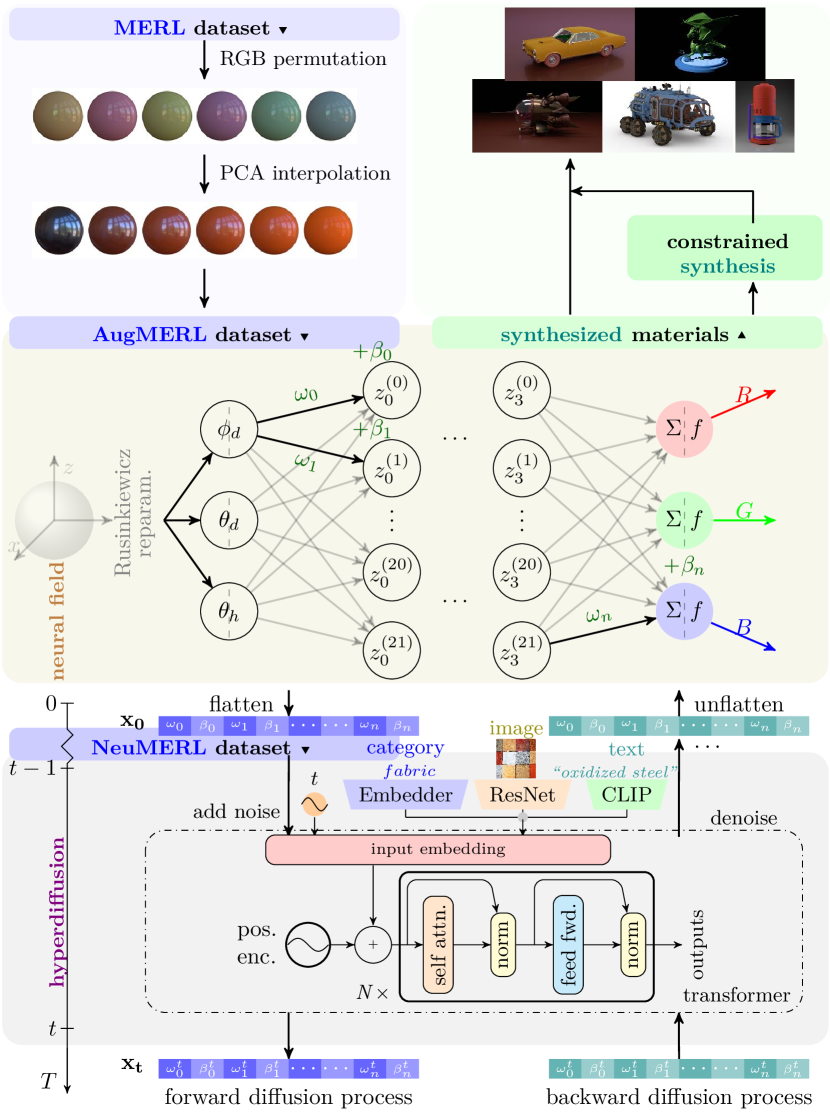
Figure 2: An overview of NeuMaDiff, our novel neural material synthesis framework, consisting of three main stages. 1 (top left): Data augmentation using RGB permutation and PCA interpolation to create an expanded dataset, AugMERL; 2 (middle): Neural field fitted to individual materials, resulting in NeuMERL, a dataset of neural material representations; and 3 (bottom): Training a multi-modal conditional hyperdiffusion model on NeuMERL to enable conditional synthesis of high-quality, diverse materials guided by inputs such as material type, text descriptions, or reference images. We further propose a novel statistics-based constrained synthesis method to generate materials of a specified type (top right).

3.1 Data Augmentation

We utilize the MERL BRDF dataset [34], which includes 100 materials, each represented by densely sampled BRDF values in a $D_{\text{MERL}}=90\times 90\times 180$-dimensional space.

Through experimentation, we determined that 100 samples are insufficient for effective hyperdiffusion training. To address this, we augment the MERL dataset using RGB permutation and PCA interpolation. First, we permute the three color channels (RGB) of each MERL sample, yielding an expanded dataset of $100\times 3!=600$ samples. An example of RGB permutation is illustrated in Fig. 3.

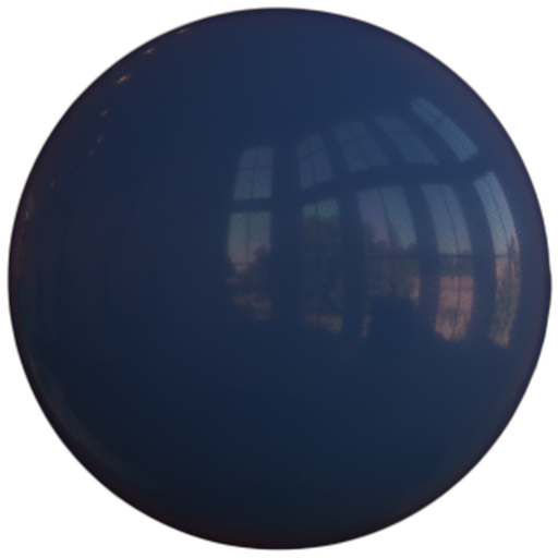
RGB

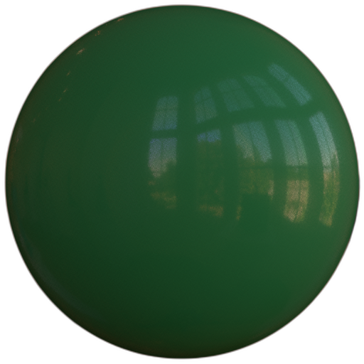
RBG

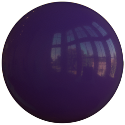
GRB

GBR

BRG

BGR

Figure 3: Six RGB permutations of the MERL material blue acrylic. (a) represents the original material. This permutation strategy expands the dataset by a factor of 6.

After applying RGB permutation, we perform principal component analysis (PCA) [1] to reduce the dimensionality of the BRDF data from $D_{\text{MERL}}$ to 300. In this lower-dimensional space, we perform linear interpolation to further augment the dataset, expanding it to $2400$ materials. Compared to direct linear interpolation in the high-dimensional BRDF space, interpolation in PCA space is more effective in capturing the underlying structure of the BRDF data and yields perceptually accurate results [34, 30, 44]. An example of materials generated through PCA interpolation is shown in Fig. 4. We refer to this augmented dataset as Augmented MERL (AugMERL). For additional details on PCA, please see Sec. A.1 in the supplementary.

0%

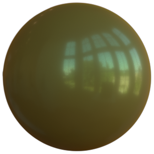
20%

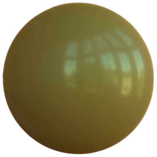
40%

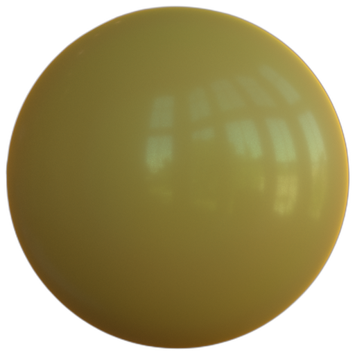
60%

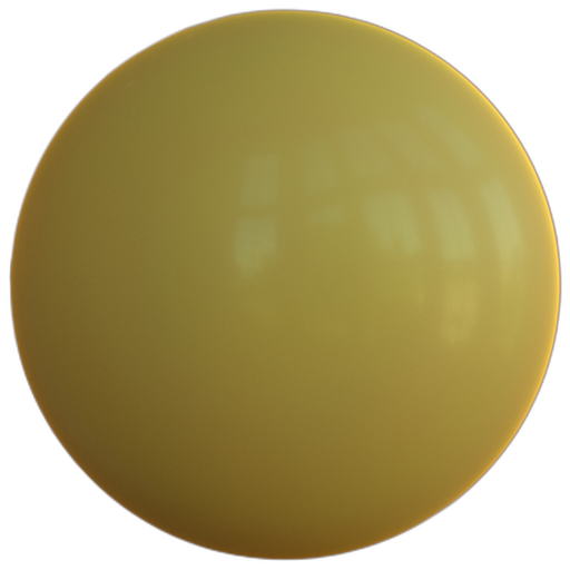
80%

100%

Figure 4: Linear interpolation of two MERL materials, (a) green metallic paint and (f) yellow plastic, in the PCA space.

3.2 Neural Field Fitting

Neural fields provide a low-dimensional, continuous representation for material data. Following prior work [49], we overfit a compact neural field $f_{r}^{{\bm{\mathbf{\xi}}}}$ parameterized by ${\bm{\mathbf{\xi}}}$, to each material in AugMERL. Once fitted, we treat the flattened weights of each neural field as the material’s neural representation. With 2400 materials in AugMERL, this process yields a dataset of 2400 neural material representations, which we refer to as Neural MERL (NeuMERL).

Representing materials as flattened 1D vectors enables a flexible framework for modeling complex distributions, abstracting away the underlying data’s dimensionality. This approach makes our pipeline adaptable to diverse data formats. In the following section, we detail three key techniques employed in fitting the neural fields.

Rusinkiewicz reparametrization

In our preliminary experiments and other studies [e.g., 63], it is observed that directly using the conventional BRDF input format – namely the incident and outgoing directions ${\bm{\mathbf{\omega}}}_{i},{\bm{\mathbf{\omega}}}_{o}\in\mathbb{R}^{3}$ – can complicate the fitting process for certain materials and occasionally introduce undesirable artifacts possibly due to the high dimensionality of the input. To address this, we employ the Rusinkiewicz reparametrization [45], which defines the half and difference vectors ${\bm{\mathbf{h}}}$ and ${\bm{\mathbf{d}}}$ as follows:

$${\bm{\mathbf{h}}} :=\frac{{\bm{\mathbf{\omega}}}_{i}+{\bm{\mathbf{\omega}}}_{o}}{\lVert{\bm{\mathbf{\omega}}}_{i}+{\bm{\mathbf{\omega}}}_{o}\rVert};$$ (1)

$${\bm{\mathbf{d}}} :=R_{\hat{{\bm{\mathbf{b}}}},-\theta_{\bm{\mathbf{h}}}}R_{\hat{{\bm{\mathbf{n}}}},-\varphi_{\bm{\mathbf{h}}}}{\bm{\mathbf{\omega}}}_{i},$$ (2)

where $R_{{\bm{\mathbf{v}}},\alpha}$ denotes a rotation around the vector ${\bm{\mathbf{v}}}$ by the angle $\alpha$, $\hat{{\bm{\mathbf{n}}}}$ is the surface normal, and $\hat{{\bm{\mathbf{b}}}}$ is the surface binormal. This reparametrization helps improve the robustness of the neural field fitting process by addressing reciprocity constraints more directly [63].

We then proceed by adopting the spherical coordinates of the half and difference vectors ${\bm{\mathbf{h}}}$ and ${\bm{\mathbf{d}}}$, specifically $\theta_{{\bm{\mathbf{h}}}},\varphi_{{\bm{\mathbf{h}}}},\theta_{{\bm{\mathbf{d}}}},\varphi_{{\bm{\mathbf{d}}}}$, as inputs to our neural fields. A further advantage of using the Rusinkiewicz reparametrization is that, since our materials are isotropic, the BRDF remains invariant with respect to $\varphi_{{\bm{\mathbf{h}}}}$. Consequently, we can omit this parameter, reducing the input complexity from $({\bm{\mathbf{\omega}}}_{i},{\bm{\mathbf{\omega}}}_{o})\in\mathbb{R}^{6}$ to $(\theta_{{\bm{\mathbf{h}}}},\theta_{{\bm{\mathbf{d}}}},\varphi_{{\bm{\mathbf{d}}}})\in[0,\frac{\pi}{2}]^{2}\times[0,\pi)$. This reparametrization enhances the efficiency of our neural field representation without sacrificing accuracy.

Mean absolute logarithmic loss

The high dynamic range of BRDF values makes fitting reflectance data particularly sensitive to error distribution. For low reflectance values, even minor fitting errors can have a large impact on the loss, causing shifts in perceived “hue” in rendered images, which leads to unrealistic colors and reduced visual fidelity. To address these issues, we employ a mean absolute logarithmic loss for BRDF values:

$$\mathcal{L}_{\text{NF}}({\bm{\mathbf{\xi}}}):=\mathbb{E}_{\raisebox{-11.38109pt}{ $\mathclap{\begin{subarray}{c}\theta_{{\bm{\mathbf{h}}}},\theta_{{\bm{\mathbf{d}}}},\varphi_{{\bm{\mathbf{d}}}}\end{subarray}}$ }}\mkern-5.0mu\Big{[}\left|\log\left(1+f_{r}\cos\theta_{i}\right)-\log\left(1+f_{r}^{{\bm{\mathbf{\xi}}}}\cos\theta_{i}\right)\right|\Big{]}$$

where $f_{r}$ denotes the ground-truth BRDF, which $f_{r}^{{\bm{\mathbf{\xi}}}}$ aims to approximate, and $\theta_{i}$ is the polar angle of the incident direction. This loss is computed per color channel, offering a balanced approach that stabilizes training across samples with both low and high values. Consequently, it enhances the model’s capability to manage dynamic reflectance variations, leading to more realistic color reproduction and improved visual fidelity.

Weight initialization

Ideally, the neural materials in NeuMERL should originate from a consistent distribution. However, due to a phenomenon known as weight symmetry [3], we observe that different weight configurations can yield the same neural field. For instance, swapping weights between two neurons in a hidden layer, or flipping the signs of both input and output weights for a neuron before an odd, linear, or piecewise-linear activation function like ReLU [37], results in an identical neural field. To address this, we propose using the optimized weights from the first fitted neural field as the initialization for subsequent neural field fittings. This approach helps align the weights across all fitted fields, promoting consistency within the NeuMERL dataset and facilitating smoother training of the hyperdiffusion model in the next stage.

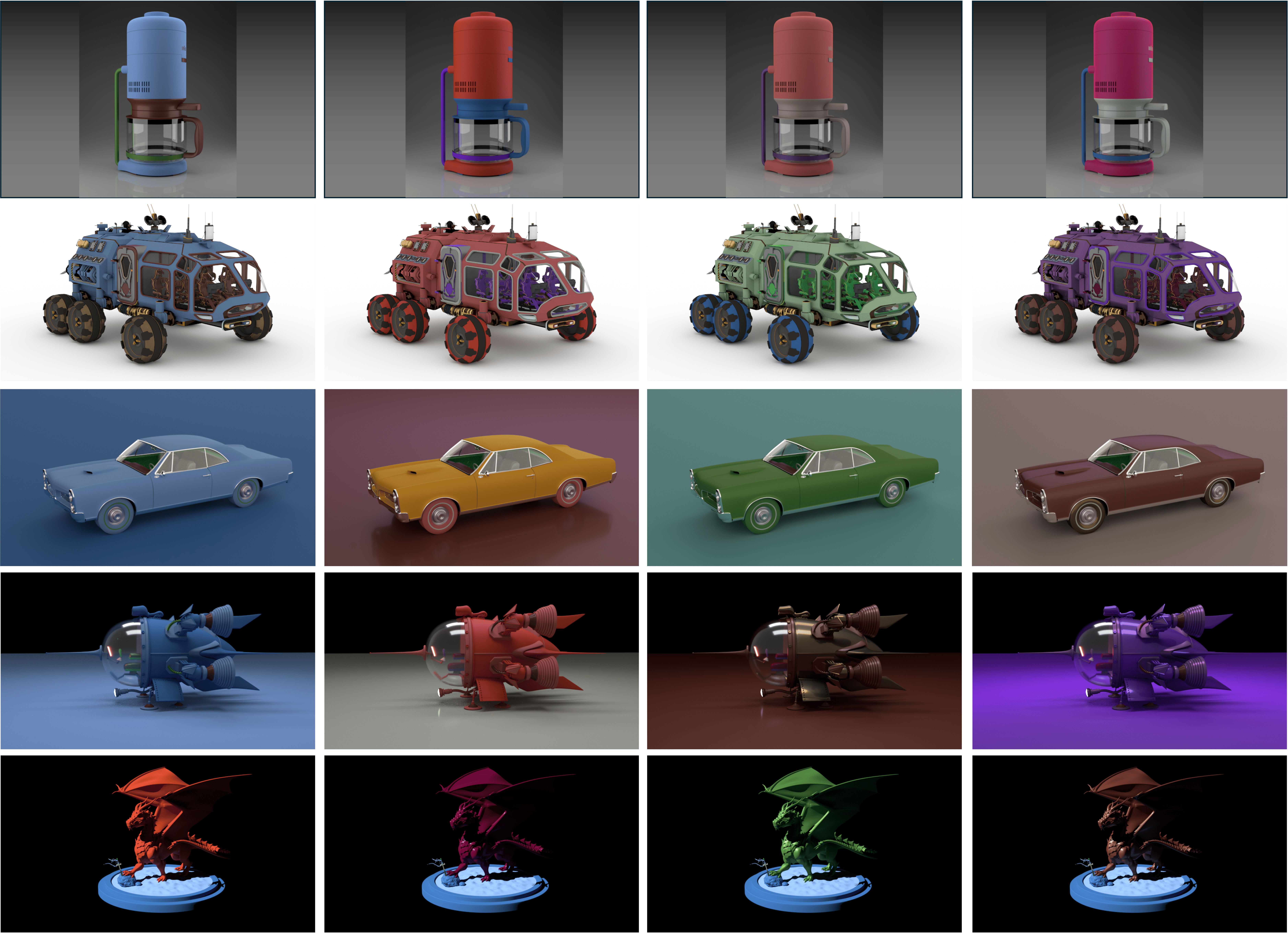
Figure 5: Renderings of different 3D models using our synthesized neural materials, highlighting the quality and diversity.

3.3 Multi-Modal Conditional Hyperdiffusion

To model the complex distribution within the NeuMERL dataset, we utilize a diffusion process [25, 41, 13]. Specifically, we employ a transformer-based denoising network [52], leveraging its demonstrated efficacy [41] and its attention mechanisms allowing for an effective focus on relevant information, enhancing the network’s ability to capture intricate dependencies in the data.

Our hyperdiffusion supports conditioning across three modalities: material type (represented as integers), text description, and reference images. For each modality, we utilize a categorical encoding for material type, an augmented CLIP text embedding [43, 62] for text, and a ResNet [22] for images. This multi-modal conditioning approach enables material synthesis to be guided by different user inputs, enhancing workflow intuitiveness and accessibility and allowing for a more smooth and accurate translation of creative vision into generated materials. For conditional sampling, we employ classifier-free guidance (CFG) [24].

Please refer to Secs. A.2, B.2, A.3 and B.3 in the supplementary for further details on the diffusion model, transformer, attention mechanism, and CFG, respectively.

4 Experiments

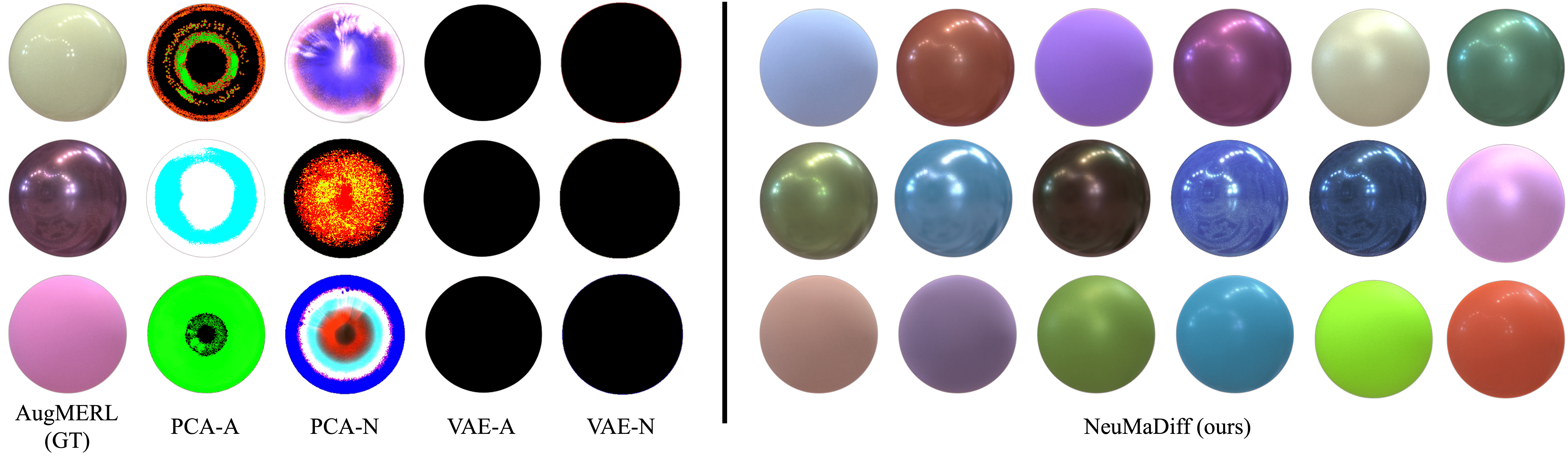
Figure 6: Material synthesis across various pipelines. All baseline models fail to capture the underlying distribution effectively, resulting in meaningless samples with severe artefacts in the synthesized materials. In contrast, NeuMaDiff successfully captures the complex neural material distribution, achieving significantly better fidelity and diversity.

In this section, we present an extensive evaluation of NeuMaDiff, beginning with an overview of our datasets (Sec. 4.1) and introducing novel material distributional metrics (Sec. 4.2). We then demonstrate the effectiveness of our pipeline through experiments on unconditional synthesis (Sec. 4.3), multi-modal conditional synthesis (Sec. 4.4), and constrained synthesis (Sec. 4.5).

For additional details, refer to the supplementary material: model implementation and training specifics are discussed in Secs. B and C.1, further results are presented in Sec. E, and Sec. F includes additional experiments.

4.1 Dataset

We fit neural fields to individual materials in the AugMERL dataset (Sec. 3.1), which is derived from the MERL BRDF dataset [34]. Our hyperdiffusion model is trained on the NeuMERL dataset (Sec. 3.2), which consists of neural material representations. The training-validation split is 80%-20% for AugMERL and 95%-5% for NeuMERL. In the constrained synthesis experiments in Sec. 4.5, statistical information is gathered from the MERL dataset [34].

4.2 Material Distributional Metrics

We use Fréchet Inception Distance (FID) [23] as an image-based metric to assess the quality of rendered single-view images by comparing them to a reference set.

To the best of our knowledge, effective metrics for directly comparing material distributions are still lacking. Drawing inspiration from distributional metrics for point clouds [2, 32, 59], we introduce three novel material distributional metrics – minimum matching distance (MMD), coverage (COV), and 1-nearest neighbor (1-NNA) – to evaluate the fidelity and diversity of synthesized BRDF sets $\mathcal{S}$ relative to a reference set $\mathcal{R}$. Each metric is based on an underlying distance measure $d(f_{r},f_{r}^{\prime})$ between two BRDFs.

Minimum matching distance (MMD)

MMD measures the average distance from each reference BRDF to its nearest synthesized counterpart:

$$\mathcal{L}_{\text{MMD}}^{d}(\mathcal{R},\mathcal{S}):=\frac{1}{\left|\mathcal{R}\right|}\sum_{f_{r}\in\mathcal{R}}\underset{f_{r}^{\prime}\in\mathcal{S}}{\min}d(f_{r},f_{r}^{\prime})$$ (3)

MMD evaluates the fidelity of the synthesized set relative to the reference, with a lower score indicating higher fidelity.

Coverage (COV)

COV calculates the proportion of reference BRDFs that are “covered” by the synthesized set. A reference BRDF is considered covered if it is the closest neighbor to at least one synthesized BRDF:

$$\mathcal{L}_{\text{COV}}^{d}(\mathcal{R},\mathcal{S})=\frac{\left|\left\{\underset{f_{r}\in\mathcal{R}}{\text{argmin }}d(f_{r},f_{r}^{\prime})\mid f_{r}^{\prime}\in\mathcal{S}\right\}\right|}{\left|\mathcal{R}\right|}$$ (4)

COV assesses the diversity of the synthesized set, with a higher score reflecting better coverage.

1-nearest neighbor (1-NNA)

1-NNA is a leave-one-out metric that measures the similarity between the reference and synthesized BRDF distributions, capturing both diversity and fidelity:

$$\mathcal{L}_{\text{1-NNA}}^{d}(\mathcal{R},\mathcal{S}):=\frac{\sum\limits_{f_{r}\in\mathcal{R}}\mathbb{I}\left[N_{f_{r}}\in\mathcal{R}\right]+\sum\limits_{f_{r}^{\prime}\in\mathcal{S}}\mathbb{I}[N_{f_{r}^{\prime}}\in\mathcal{S}]}{\left|\mathcal{S}\right|+\left|\mathcal{R}\right|},$$ (5)

where $\mathbb{I}[\cdot]$ is the indicator function and $N_{f_{r}}$ denotes the nearest neighbor of $f_{r}$ in $(\mathcal{R}\cup\mathcal{S})-\{f_{r}\}$. In this metric, each sample is classified as belonging to either the reference set $\mathcal{R}$ or the synthesized set $\mathcal{S}$ based on the membership of its nearest neighbor. If $\mathcal{R}$ and $\mathcal{S}$ are drawn from the same underlying distribution, the classifier’s accuracy will approach 50% with a large sample size. An accuracy closer to 50% indicates greater similarity between $\mathcal{R}$ and $\mathcal{S}$, suggesting that the model has effectively learned the target distribution.

Each distributional metric can be computed using an underlying distance $d$. Potential options include rendering-based metrics such as root mean squared error (RMSE), peak signal-to-noise ratio (PSNR), and structural similarity index measure (SSIM) [54]. PSNR measures the reconstruction quality of images, while SSIM predicts perceived similarity. Since higher values in PSNR and SSIM correspond to greater similarity, we negate these values – resulting in NegPSNR and NegSSIM, respectively – to make them plausible distance functions. To directly assess the distance between two BRDFs without relying on renderings, we also introduce the following BRDF-L1 distance:

$$d_{\text{BRDF-L1}}:=\underset{\theta_{{\bm{\mathbf{h}}}},\theta_{{\bm{\mathbf{d}}}},\varphi_{{\bm{\mathbf{d}}}}}{\mathbb{E}}\Big{[}\left|f_{r}-f_{r}^{\prime}\right|\Big{]};$$ (6)

For further background on the image-based metrics and validation of the proposed material distributional metrics, please refer to Sec. D in the supplementary.

4.3 Unconditional Synthesis

We begin by presenting the results of unconditional synthesis of neural materials using NeuMaDiff. Most existing approaches utilize principal component analysis (PCA) [1, 48] and variational autoencoders (VAEs) [28, 17]. Accordingly, we developed four generative baselines based on the two methods PCA and VAE. Each method was applied to either the AugMERL or NeuMERL datasets, resulting in the following baselines: PCA-A, PCA-N, VAE-A, and VAE-N. For synthesis, PCA-based baselines perform random linear interpolation in the principal space, while VAE-based baselines sample from a standard Gaussian prior. Additional background details on these methods can be found in Secs. A.4 and B.4 in the supplementary material.

Table 1 provides a detailed comparison of synthesized materials using our proposed metrics, while Figs. 6, 5 and 1 showcase renderings of these materials across various scenes, from simple spheres to more complex models. The quantitative and qualitative results indicate that NeuMaDiff consistently outperforms all baselines across metrics, producing diverse, high-quality, visually appealing, and perceptually realistic renderings. This demonstrates the effectiveness of NeuMaDiff for neural material synthesis. Notably, materials synthesized by the PCA- and VAE-based baselines exhibit significant artifacts, likely due to the limitations of these simpler models in capturing the complex distribution of neural materials.

Metric		Training set	PCA-A	PCA-N	VAE-A	VAE-N	NeuMaDiff (ours)
FID ($\downarrow$)		0.187	10.9	23.8	26.1	28.4	0.440
MMD ($\downarrow$)	BRDF-L1$\times 10^{-3}$	2.51	9.05	9.22	9.09	$\infty$	4.02
	RMSE$\times 10^{2}$	7.54	33.3	30.2	63.7	69.2	9.34
	NegPSNR	$-$28.7	$-$13.9	$-$14.8	$-$8.30	$-$7.40	$-$25.6
	NegSSIM$\times 10$	$-$9.55	$-$6.74	$-$6.29	$-$2.68	$-$2.15	$-$9.40
COV (%) ($\uparrow$)	BRDF-L1	60.8	2.50	30	0.833	2.50	50.8
	RMSE	55.8	18.3	28.3	0.833	0.833	50.0
	NegPSNR	56.7	18.3	28.3	0.833	0.833	50.0
	NegSSIM	59.2	23.3	16.7	0.833	0.833	51.7
1-NNA (%) ($\downarrow$)	BRDF-L1	58.8	100	95.4	100	100	80.0
	RMSE	55.4	96.3	93.4	100	100	60.0
	NegPSNR	55.0	94.2	90.0	100	100	60.4
	NegSSIM	57.5	96.3	96.7	100	100	61.7

Table 1: Qualitative evaluation of unconditional synthesis with metrics assessing generation fidelity and diversity. $\downarrow$ indicates that a lower score is better and $\uparrow$ indicates the opposite. NeuMaDiff significantly outperforms all baseline models across these metrics, underscoring its effectiveness in neural material synthesis.

4.4 Multi-Modal Conditional Synthesis

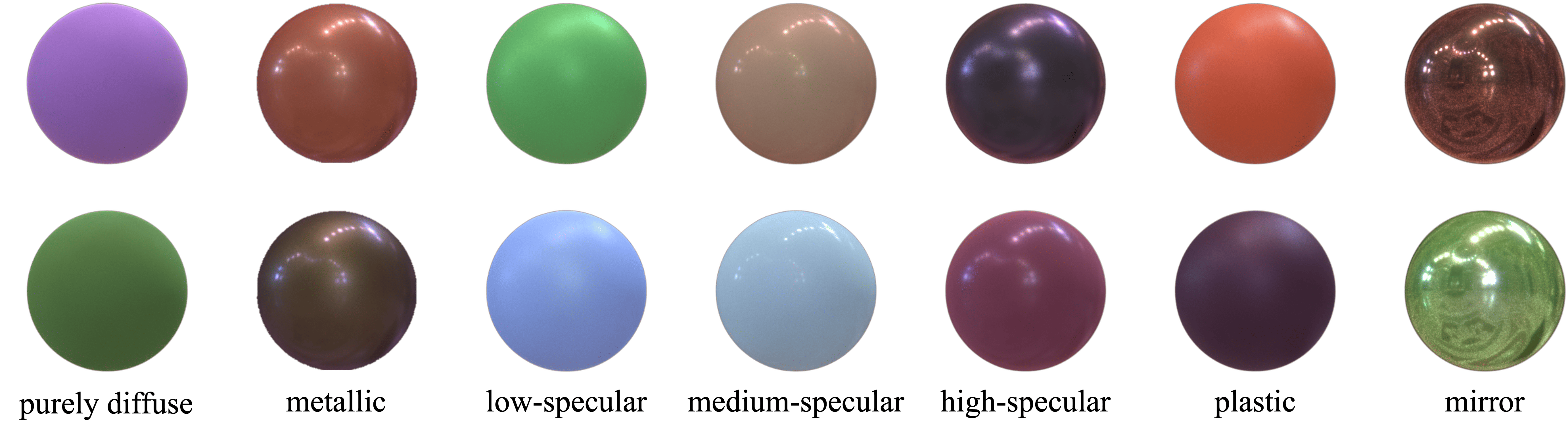
Figure 7: Synthesized materials of seven distinct categories using our novel constrained synthesis. Grounded in BRDF statistical analysis, this approach provides enhanced explainability and interpretability compared to standard conditional synthesis methods.

To further evaluate the effectiveness of our pipeline, we perform multi-modal conditional synthesis by conditioning our model on various modalities of input: material type, text description, or material images.

For material type conditioning, we represent each of the 48 material types in the MERL dataset [34] (e.g., acrylic, aluminium, metallic, plastic, etc.) using integers. The full list of material types is available in Sec. C.2 in the supplementary; For text-based conditioning, we use descriptions derived from the MERL dataset materials [34]. For additional materials in the AugMERL dataset, descriptions are assigned as follows: For RGB-permuted materials, we retain the original description but omit color-specific words (e.g., “red metallic paint” becomes “metallic paint”); For PCA-interpolated materials, we generate descriptions in the format “a mixture of $t_{A}$ and $t_{B}$”, where $t_{A}$ and $t_{B}$ are the descriptions of the interpolated materials $A$ and $B$, respectively; For image-based conditioning, we use cropped single-view renderings of materials from AugMERL as input to guide the synthesis based on visual references.

Figures 8, 9 and 10 present the results for type-, text-, and image-conditioned synthesis, respectively. Across all conditioning modes, the synthesized materials demonstrate realism, diversity, and a close alignment with the input conditions. Notably, in text-conditioned synthesis, NeuMaDiff effectively generalizes to novel inputs, such as “green metal”, “red plastic”, and “highly specular material”, producing materials that are perceptually consistent with these previously unseen descriptions.

Figure 8: Type-conditioned synthesis. The synthesized materials are diverse and closely align with the specified material type.

Figure 9: Text-conditioned synthesis. NeuMaDiff synthesizes materials aligning with the texts and generalizes to unseen inputs: “green metal”, “red plastic”, and “highly specular material”.

Figure 10: Image-conditioned synthesis. In each of the six pairs, the left image is the conditioning input, while the right image is the synthesized result. NeuMaDiff effectively generates realistic materials that closely align with the conditioning images.

4.5 Constrained Synthesis

We classify materials into seven categories based on their reflective properties: diffuse, metallic, low-specular, medium-specular, high-specular, plastic, and mirror. To enable the synthesis of materials within a specified category, we introduce a novel approach called constrained synthesis. This statistics-based method complements our conditional pipeline by enforcing constraints on unconditionally synthesized samples, allowing for targeted material generation according to desired reflective characteristics.

We derive the theoretical upper limit for a diffuse reflectance value, $f_{\text{diffuse}}$, for a constant (i.e., purely diffuse) BRDF $f_{r}({\bm{\mathbf{\omega}}}_{i},{\bm{\mathbf{\omega}}}_{o})\equiv f_{\text{diffuse}}$ in each color channel. For a physically valid BRDF that adheres to energy passivity [63], the reflected energy must not exceed the incident energy in each channel. Thus, we have:

$$1 \geq\int_{H^{2}}f_{r}({\bm{\mathbf{\omega}}}_{i},{\bm{\mathbf{\omega}}}_{o})\cos\theta_{o}\,\mathrm{d}{\bm{\mathbf{\omega}}}_{o}$$ (7)

$$=f_{\text{diffuse}}\int_{H^{2}}\cos\theta_{o}\,\mathrm{d}{\bm{\mathbf{\omega}}}_{o}=\pi f_{\text{diffuse}}$$ (8)

$$\Rightarrow f_{\text{diffuse}}\leq\frac{1}{\pi}.$$ (9)

Building on this observation and a statistical analysis of the MERL’s mean and maximum reflectance values across color channels and material types (Sec. F.1 in the supplementary), we propose a novel set of rules for categorizing materials into seven types. These rules enable the constrained selection of synthesized materials based on desired material characteristics. Unlike many black-box machine learning approaches, this method is rooted in BRDF analysis, offering inherent explainability and interpretability. Below, we outline two of these rules, with the full set detailed in Sec. C.3.

• Purely diffuse materials: The reflectance values in all directions do not exceed the diffuse threshold $f_{\text{diffuse}}$, allowing for only $e:=8\times 10^{4}$ exceptions:

  $$\lvert\{({\bm{\mathbf{\omega}}}_{o},{\bm{\mathbf{\omega}}}_{i})\in\mathbb{R}^{6}\mid\left\|f_{r}({\bm{\mathbf{\omega}}}_{o},{\bm{\mathbf{\omega}}}_{i})\right\|_{\infty}>f_{\text{diffuse}}\}\rvert<e,$$ (10)

  where $\left\|\cdot\right\|_{\infty}$ denotes the maximum reflectance value among the three color channels.

• Metallic materials: The reflectance values in all directions exceed the diffuse threshold $f_{\text{diffuse}}$:

  $$\forall({\bm{\mathbf{\omega}}}_{o},{\bm{\mathbf{\omega}}}_{i})\in\mathbb{R}^{6},\left\|f_{r}({\bm{\mathbf{\omega}}}_{o},{\bm{\mathbf{\omega}}}_{i})\right\|_{\infty}>f_{\text{diffuse}}$$ (11)

Figure 7 shows materials generated through our constrained synthesis, incorporating the proposed filtering rules to ensure that the synthesized outputs match the specified material categories. The results demonstrate that the synthesized materials effectively exhibit the characteristics of the desired categories.

5 Conclusion and Discussion

High-quality material synthesis is critical for achieving realistic, convincing renderings. In this work, we introduced NeuMaDiff, an innovative neural material synthesis pipeline built upon a multi-modal conditional hyperdiffusion model. Using neural fields as the core representation for materials, we trained our hyperdiffusion on their weights, demonstrating its effectiveness in generating high-quality, diverse materials through extensive experiments. Additionally, we contribute two material datasets and two BRDF distributional metrics to facilitate future research.

However, our current evaluation is limited to uniform material datasets. Extending our approach to accommodate more complex materials, such as spatially varying BRDFs, may require additional mechanisms, which we aim to explore in future work.

Supplementary Material

A Additional Background

A.1 Principal Component Analysis

Principal component analysis (PCA) [1], also known as Karhunen-Loève transform or Hotelling transform, is a linear dimensionality reduction technique. We utilize PCA for data augmentation in Sec. A.1 and baseline models in Sec. 4.3.

Given a dataset of $n$ samples in a high-dimensional space $\mathcal{D}\in\mathbb{R}^{n\times d}$, PCA seeks to linearly transform the data onto a lower-dimensional space $\mathbb{R}^{k}$ spanned by $k$ principal components capturing the primary variance of the data. In this reduced space, synthetic data points are generated by sampling from a Gaussian distribution with the same mean and variance as the original data in each principal component direction. These newly sampled points are then mapped back to the original feature space using the inverse PCA transformation. This method allows the creation of new data samples that maintain the underlying structure and variance characteristics of the original dataset, which can be useful for data augmentation and improving model robustness.

A.2 Diffusion Model

The forward and backward processes in hyperdiffusion are modeled as Markov chains with a total timestep $T$ and learnable parameter ${\bm{\mathbf{\eta}}}$:

$$q({\bm{\mathbf{x}}}_{1},\ldots,{\bm{\mathbf{x}}}_{T}|{\bm{\mathbf{x}}}_{0})=\prod_{t=1}^{T}q({\bm{\mathbf{x}}}_{t}|{\bm{\mathbf{x}}}_{t-1}),$$ (12)

$$p_{\bm{\mathbf{\eta}}}({\bm{\mathbf{x}}}_{0},\ldots,{\bm{\mathbf{x}}}_{T})=p_{\bm{\mathbf{\eta}}}({\bm{\mathbf{x}}}_{t})\prod_{t=1}^{T}p_{\bm{\mathbf{\eta}}}({\bm{\mathbf{x}}}_{T}|{\bm{\mathbf{x}}}_{t-1}).$$ (13)

In the forward process, starting with the original data ${\bm{\mathbf{x}}}={\bm{\mathbf{x}}}_{0}$, we iteratively add Gaussian noise at each step:

$$q({\bm{\mathbf{x}}}_{t}|{\bm{\mathbf{x}}}_{t-1}):=\mathcal{N}({\bm{\mathbf{x}}}_{t};\sqrt{1-\beta_{t}}{\bm{\mathbf{x}}}_{t-1},\beta_{t}I),$$ (14)

where $\{\beta_{t}\}_{t=1}^{T}$ defines the variance schedule. Each noisy vector, paired with the sinusoidal embedding of the timestep, is passed through a linear projection layer. The output projections are then combined with a learnable positional encoding vector. As the forward process progresses, $p({\bm{\mathbf{x}}}_{T})$ converges towards a standard Gaussian distribution, $\mathcal{N}(0,I)$.

In the backward process, the transformer takes these inputs and produces denoised tokens, which are passed through a final output projection layer to generate the predicted noise. To train a learnable model ${\bm{\mathbf{\epsilon}}}_{\bm{\mathbf{\eta}}}({\bm{\mathbf{x}}}_{t},t)$ parameterized by ${\bm{\mathbf{\eta}}}$, we minimize the score matching objective:

$$\mathcal{L}_{\text{HD}}({\bm{\mathbf{\eta}}}):=\mathbb{E}_{{\bm{\mathbf{x}}}_{0},t\sim\mathcal{U}(1,T),{\bm{\mathbf{\epsilon}}}\sim\mathcal{N}(0,I)}\left[\|{\bm{\mathbf{\epsilon}}}-{\bm{\mathbf{\epsilon}}}_{\bm{\mathbf{\eta}}}({\bm{\mathbf{x}}}_{t},t)\|_{2}^{2}\right],$$ (15)

where $\mathcal{U}(1,T)$ represents the uniform distribution over $\{1,2,\ldots,T\}$. This objective encourages the model to accurately predict the noise ${\bm{\mathbf{\epsilon}}}$, effectively guiding the denoising process.

During inference, the network enables sampling via an iterative process [47], leveraging the factorization of the learned distribution as

$$p_{\bm{\mathbf{\eta}}}({\bm{\mathbf{x}}})=p({\bm{\mathbf{x}}}_{T})p_{\bm{\mathbf{\eta}}}({\bm{\mathbf{x}}}_{0}|{\bm{\mathbf{x}}}_{T})=p({\bm{\mathbf{x}}}_{T})\prod_{t=1}^{T}p_{\bm{\mathbf{\eta}}}({\bm{\mathbf{x}}}_{t-1}|{\bm{\mathbf{x}}}_{t})$$ (16)

for $p({\bm{\mathbf{x}}}_{T}):=\mathcal{N}(0,I)$. For conditional sampling, we employ classifier-free guidance (CFG) [24] (for more details, please refer to Sec. B.3).

A.3 Attention Mechanism

The attention mechanism [52] allows models to focus on specific parts of input data, dynamically assigning different levels of “attention” or importance to different elements. Attention mechanisms enable models to learn which parts of the input sequence are most relevant to predicting each output token. This process improves performance by allowing models to prioritize relevant information and ignore irrelevant details, especially in long sequences.

In modern applications, attention modules are widely used in natural language processing (NLP), computer vision, and beyond. The transformer architecture [52], which relies heavily on the self-attention mechanism, has become foundational in NLP models, including BERT [11] and GPT [33]. Attention allows these models to capture complex dependencies between words in a sentence, regardless of their distance from each other, leading to significant advancements in tasks like language translation, sentiment analysis, and image processing.

The attention mechanism computes a weighted combination of values based on the relevance of each value to a given query. In the context of self-attention (or scaled dot-product attention) in transformer models [52], this process involves three main components: queries (${\bm{\mathbf{q}}}$), keys (${\bm{\mathbf{k}}}$), and values (${\bm{\mathbf{v}}}$). In summary, the attention mechanism dynamically focuses on relevant parts of the input by computing similarity scores between queries and keys, normalizing these scores, and using them to weight the values. This allows models to capture dependencies across elements in a sequence, making attention a powerful tool for handling long-range dependencies in data.

Given an input sequence of embeddings ${\bm{\mathbf{X}}}$ (e.g., word embeddings in NLP or patch embeddings in vision), we first transform it into three different linear projections:

$${\bm{\mathbf{q}}} ={\bm{\mathbf{X}}}W_{\bm{\mathbf{q}}};$$ (17)

$${\bm{\mathbf{k}}} ={\bm{\mathbf{X}}}W_{\bm{\mathbf{k}}};$$ (18)

$${\bm{\mathbf{v}}} ={\bm{\mathbf{X}}}W_{\bm{\mathbf{v}}},$$ (19)

where $W_{\bm{\mathbf{q}}}$, $W_{\bm{\mathbf{k}}}$, and $W_{\bm{\mathbf{v}}}$ are learnable weight matrices. These projections represent the queries, keys, and values, respectively. The attention score between each query and key is then computed as the dot product ${\bm{\mathbf{q}}}\cdot{\bm{\mathbf{t}}}$. This results in a matrix of scores that represents the similarity between each element in the sequence. To stabilize gradients and prevent large values in the dot-product computation, the scores are scaled by the square root of the dimensionality of the queries/keys $\sqrt{d_{\bm{\mathbf{k}}}}$, where $d_{\bm{\mathbf{k}}}$ is the dimension of the key vectors. The scaled scores are $\frac{{\bm{\mathbf{q}}}\cdot{\bm{\mathbf{t}}}}{\sqrt{d_{k}}}$.

The scaled scores are passed through a softmax function, producing attention weights that sum to 1. This step converts the scores into probabilities, indicating the relevance of each value with respect to each query. These attention weights are used to compute a weighted sum of the values. Specifically, the output of the attention mechanism is

$$f_{\text{attention}}({\bm{\mathbf{q}}},{\bm{\mathbf{k}}},{\bm{\mathbf{v}}})=f_{\text{softmax}}\left(\frac{{\bm{\mathbf{q}}}\cdot{\bm{\mathbf{k}}}}{\sqrt{d_{k}}}\right){\bm{\mathbf{v}}}.$$ (20)

This produces a context vector for each query that incorporates information from all other elements in the sequence, weighted by their relevance.

In practice, multiple attention heads are used in parallel. Each head learns different aspects of the input by using different projections $W_{\bm{\mathbf{q}}},W_{\bm{\mathbf{k}}},$ and $W_{\bm{\mathbf{v}}}$. The outputs from each head are then concatenated and linearly transformed to produce the final output.

A.4 Variational Autoencoder

We adopt variational autoencoders (VAEs) [28] as one of the baseline models in Sec. 4.3. VAEs are probabilistic generative models designed to capture the underlying probability distribution of a given dataset $\mathcal{D}$.

A VAE consists of a parameterized encoder $q_{{\bm{\mathbf{\psi}}}}({\bm{\mathbf{z}}}|{\bm{\mathbf{x}}})$ and decoder $p_{{\bm{\mathbf{\zeta}}}}({\bm{\mathbf{x}}}|{\bm{\mathbf{z}}})$, defined by parameters ${\bm{\mathbf{\psi}}}$ and ${\bm{\mathbf{\zeta}}}$, respectively. Assuming that the latent variables ${\bm{\mathbf{z}}}\in\mathbb{R}^{D_{\bm{\mathbf{z}}}}$ follow a prior distribution $p({\bm{\mathbf{z}}})$, both the encoder and decoder are jointly optimized to maximize the evidence lower bound (ELBO) on the likelihood of the data:

$$\mathcal{L}_{\text{ELBO}}({\bm{\mathbf{\psi}}},{\bm{\mathbf{\zeta}}};{\bm{\mathbf{x}}}):= \mathbb{E}{q_{{\bm{\mathbf{\psi}}}}({\bm{\mathbf{z}}}|{\bm{\mathbf{x}}})}\left[\log p_{{\bm{\mathbf{\zeta}}}}({\bm{\mathbf{x}}}|{\bm{\mathbf{z}}})\right]$$ (21)

$$-\mathcal{D}_{\text{KL}}\left(q_{{\bm{\mathbf{\psi}}}}({\bm{\mathbf{z}}}|{\bm{\mathbf{x}}}),p({\bm{\mathbf{z}}})\right),$$

where $\mathcal{D}_{\text{KL}}$ represents the Kullback-Leibler divergence between the approximate posterior and the prior distribution [9]. This probabilistic framework enables VAEs to effectively approximate the true data distribution, facilitating robust generative modeling of complex data.

A.5 K-Means Clustering

We adopt K-means clustering in constrained synthesis, where unconditional materials are filtered out by statistical information rather than a neural network. K-means clustering is a commonly used unsupervised method to partition $n$ data samples ${\bm{\mathbf{X}}}\in\mathbb{R}^{n\times p}$ into $k$ clusters $\mathcal{S}=\{S_{1},...,S_{k}\}$, minimizing the distance between each sample and its center

$$\mu_{i}=\frac{1}{|S_{i}|}\sum_{\mathbf{x_{i}}\in S_{i}}\mathbf{x_{i}}.$$ (22)

The optimal partition can be computed via the following objective

$$\mathcal{S}^{*}=\arg\min_{\mathcal{S}}\sum_{i=0}^{k-1}\sum_{\mathbf{x_{i}}\in S_{i}}||\mathbf{x_{i}}-\mu_{i}||^{2}.$$ (23)

Given the assigned clusters, we can obtain the classification decision boundary directly.

B Model Details

B.1 Neural Field

The sum $D_{\text{NF}}$ of dimensionalities of the weights in our neural field $f_{r}^{\bm{\mathbf{\xi}}}$ is 675.

B.2 Transformer Backbone in Hyperdiffusion

The input and output tokens are mapped to vectors with learnable embedders. Sinusoidal positional encoding is also used. The feed-forward networks are single layer MLPs with ReLU activation functions.

The encoder network contains multiple identical layers, each with a feed-forward sublayer after multi-head attention. A residual connection is employed for each sublayer, followed by the layer normalization. The decoder is similar, but with an extra per-layer multi-head attention at the end, receiving the the encoder output.

Fig. 11 illustrates the transformer architecture.

Figure 11: Transformer as hyperdiffusion backbone.

B.3 Conditional Sampling with Classifier-Free Guidance

We employ classifier-free guidance (CFG) [24] for conditional sampling on the hyperdiffusion. We present the algorithm in Alg. 1. Notice that we require $\omega>-1$ for conditional generation. Otherwise, the model downgrades to unconditional synthesis when $\omega=-1$.

Algorithm 1 Conditional sampling with classifier-free guidance (CFG)

total timestep $T$

guidance scale $\omega\geq-1$

conditional context ${\bm{\mathbf{y}}}$

variance schedule $\{\beta_{t}\}_{t=1}^{T}$

${\bm{\mathbf{x}}}_{T}\sim\mathcal{N}(0,I_{D_{\text{NF}}})$ $\triangleright$ sample ${\bm{\mathbf{x}}}_{T}$ from prior

for $t=T$ to $1$ do

       ${\bm{\mathbf{\epsilon}}}_{\bm{\mathbf{\eta}}}^{\text{CFG}}({\bm{\mathbf{x}}}_{t},{\bm{\mathbf{y}}},t)=(1+\omega){\bm{\mathbf{\epsilon_{\eta}}}}({\bm{\mathbf{x}}}_{t},{\bm{\mathbf{y}}},t)-\omega{\bm{\mathbf{\epsilon_{\eta}}}}({\bm{\mathbf{x}}}_{t},\emptyset,t)$

       $\alpha_{t}=\prod_{i=1}^{t}\sqrt{1-\beta_{i}}$

       $\gamma_{t}=\prod_{t=1}^{t}\alpha_{t}$

       ${\bm{\mathbf{x}}}_{t}^{\text{CFG}}=\frac{1}{\sqrt{\gamma_{t}}}({\bm{\mathbf{x}}}_{t}-\sqrt{1-\gamma_{t}}{\bm{\mathbf{\epsilon_{\eta}^{\text{CFG}}}}}({\bm{\mathbf{x}}}_{t},{\bm{\mathbf{y}}},t))$

       ${\bm{\mathbf{x}}}_{t-1}=\sqrt{\gamma_{t-1}}{\bm{\mathbf{x}}}_{t}^{\text{CFG}}+\sqrt{1-\gamma_{t-1}}{{\bm{\mathbf{\epsilon_{\eta}^{\text{CFG}}}}}({\bm{\mathbf{x}}}_{t},{\bm{\mathbf{y}}},t)}$

end for

return ${\bm{\mathbf{x}}}_{0}$

B.4 PCA-Based Baselines

For PCA-based baselines introduced in the unconditional synthesis in Sec. 4.3, the dimensionalities of the reduced spaces for PCA-A and PCA-N are 300 and 100, respectively.

B.5 VAE-Based Baselines

In this section, we introduce the model and training hyperparameters for VAE-based baselines introduced in the unconditional synthesis in Sec. 4.3.

For VAE-A, to reduce the input complexity, we downsample it from $90\times 90\times 180$ to $45\times 45\times 90$ and upsample the synthetic results using nearest neighbor algorithm. The hidden dimension is 256 and the latent space dimension is 300. The model is trained with batch size 16, learning rate $5\times 10^{-3}$ until convergence.

For VAE-N, the VAE architecture contains MLP-based encoder and decoder, each with 4 layers. The input dimension is $D_{\text{NF}}$, and the hidden and the latent space dimensions are both 100. The likelihood of the reconstructed data is measured by the mean squared error (MSE). The model is trained with batch size 32, learning rate $10^{-3}$ until convergence.

C Experiment Details

C.1 Training Details

In the neural field fitting, we set the batch size to be 512, the number of epochs to be 100, and the learning rate to be $5\times 10^{-3}$.

When training the hyperdiffusion model, we set the total timestep $T$ to be 100, the batch size to be 512, the number of epochs to be 700 for unconditional synthesis and an additional 200 for conditional synthesis, and the learning rate to be adaptive from $5\times 10^{-4}$ to $5\times 10^{-6}$.

C.2 Full Material Type List

We include the full list of 48 material types used in the type-conditional synthesis in Sec. 4.4: acrylic, alum-bronze, alumina-oxide, aluminium, aventurnine, brass, wood, chrome-steel, chrome, colonial-maple, color-changing-paint, delrin, diffuse-ball, fabric, felt, fruitwood, grease-covered-steel, hematite, ipswich-pine, jasper, latex, marble, metallic-paint, natural, neoprene-rubber, nickel, nylon, obsidian, oxidized-steel, paint, phenolic, pickled-oak, plastic, polyethylene, polyurethane-foam, pvc, rubber, silicon-nitrade, soft-plastic, special-walnut, specular-fabric, specular-phenolic, specular-plastic, stainless-steel, steel, teflon, tungsten-carbide, two-layer

C.3 Full Set of Constrained Synthesis Rules

We include the full set of seven rules used in constrained synthesis:

• Purely diffuse materials: the reflectance values from all directions do not exceed the diffuse threshold $f_{\text{diffuse}}$, with only $e:=8\times 10^{4}$ exceptions:

  $$\lvert\{({\bm{\mathbf{\omega}}}_{o},{\bm{\mathbf{\omega}}}_{i})\in\mathbb{R}^{6}\mid\left\|f_{r}({\bm{\mathbf{\omega}}}_{o},{\bm{\mathbf{\omega}}}_{i})\right\|_{\infty}>f_{\text{diffuse}}\}\rvert<e,$$ (24)

  where $\left\|\cdot\right\|$ is the $\ell^{\infty}$-norm that selects the maximum component from the three color channels of reflectance values.

• Metallic materials: the reflectance values from all directions exceeds the diffuse threshold $f_{\text{diffuse}}$:

  $$\forall({\bm{\mathbf{\omega}}}_{o},{\bm{\mathbf{\omega}}}_{i})\in\mathbb{R}^{6},\left\|f_{r}({\bm{\mathbf{\omega}}}_{o},{\bm{\mathbf{\omega}}}_{i})\right\|_{\infty}>f_{\text{diffuse}}$$ (25)

• Specular materials: Through our statistical analysis, we identify two specular thresholds $f_{\text{specular}}^{(1)}:=100$ and $f_{\text{specular}}^{(2)}:=600$. The materials can be classified as low-, mid-, or high-specular if the maximum reflectance value fall in the range $[f_{\text{diffuse}},f_{\text{specular}}^{(1)}),[f_{\text{specular}}^{(1)},f_{\text{specular}}^{(2)})$, and $[f_{\text{specular}}^{(2)},\infty)$, respectively.

• Plastic materials: materials whose specular part is white. In other words, if the reflectance value exceeds $f_{\text{diffuse}}$ for some direction, the difference between any two color channels should be smaller than a tolerance $\delta_{\text{plastic}}$, which we set to be 5% of the maximum reflectance value.

• Mirror-like materials: the specular lobe in the polar diagram is narrow. In order to quantify this, we observe that under the Rusinkiewicz reparametrization (Sec. 3.2), the evaluation at $f_{r}(\theta_{{\bm{\mathbf{h}}}}=0,\theta_{{\bm{\mathbf{d}}}}=0,\varphi_{{\bm{\mathbf{d}}}}=0)$ is the peak of the lobe. Incrementing $\theta_{\bm{\mathbf{h}}}$ decreases the BRDF. The width $w$ of the lobe can then be defined as the value of $\theta_{\bm{\mathbf{h}}}$ for which the reflectance value drops to half of the the peak $\frac{f_{r}(0,0,0)}{2}$. Empirically, we found that if the width $w<w_{\text{mirror}}:=0.349$, the material exhibits mirror-like behavior.

D Metric Details

D.1 Rendering-Based Metrics

Given two rendered images $I_{1},I_{2}\colon\mathbb{R}^{w}\times\mathbb{R}^{h}\rightarrow[0,1]^{c}$, where $w,h$ are the width and height of the images, respectively, and $C$ is the number of channels, we propose the following rendering-based metrics assessing the similarity and reconstruction quality between the two images.

Root mean squared error (RMSE)

RMSE checks if pixel values at the same coordinates match.

$$\mathcal{L}_{\text{RMSE}}(I_{1},I_{2}):=\sqrt{\frac{1}{wh}{\sum_{i=1}^{w}\sum_{j=1}^{h}\left(I_{1}(i,j)-I_{2}(i,j)\right)^{2}.}}$$

Note that RMSE depends strongly on the image intensity scaling. RMSE aims for lower value for better performance.

Peak signal-to-noise ratio (PSNR)

is the scaled mean squared error (MSE). Given the maximum pixel value $p$, i.e., peak signal, PSNR is defined as

$$\mathcal{L}_{\text{PSNR}}(I_{1},I_{2})=10\log_{10}\frac{p^{2}}{\mathcal{L}_{\text{RMSE}}^{2}(I_{1},I_{2})}.$$

PSNR measures the image reconstruction quality and aims for higher values.

Structural similarity index measure (SSIM)

SSIM [54] is a perception-based metric that measures the perceptual similarity of the two images. The computation of SSIM is based on three comparison measurements between the two images: luminance ($l$), contrast ($c$), and structure ($s$) defined as

$$l(I_{1},I_{2}):=\frac{2\mu_{x}\mu_{y}+c_{1}}{\mu_{x}^{2}+\mu_{y}^{2}+c_{1}};$$ (26)

$$c(I_{1},I_{2}):=\frac{2\sigma_{I_{1}}\sigma_{I_{2}}+c_{2}}{\sigma_{I_{1}}^{2}+\sigma_{I_{2}}^{2}+c_{2}};$$ (27)

$$s(I_{1},I_{2}):=\frac{\sigma_{I_{1}I_{2}}+c_{3}}{\sigma_{I_{1}}\sigma_{I_{2}}+c_{3}},$$ (28)

respectively, where $\mu_{I},\sigma_{I}$, and $\sigma_{I_{1}I_{2}}$ are the mean, standard deviation, and variance of the images:

$$\mu_{I}:=\frac{1}{w\cdot h}{\sum_{i=1}^{w}\sum_{j=1}^{h}I(i,j)};$$ (29)

$$\sigma_{I}:=\sqrt{\frac{1}{w\cdot h-1}{\sum_{i=1}^{w}\sum_{j=1}^{h}\left(I(i,j)-\mu_{I}\right)^{2}}};$$ (30)

$$\sigma_{I_{1}I_{2}}:=\frac{1}{w\cdot h-1}\sum_{i=1}^{w}\sum_{j=1}^{h}\left(I_{1}(i,j)-\mu_{I_{1}})(I_{2}(i,j)-\mu_{I_{2}}\right)$$ (31)

and

$$c_{1}:=(k_{1}L)^{2};$$ (32)

$$c_{2}:=(k_{2}L)^{2};$$ (33)

$$c_{3}:=\frac{c_{2}}{2}$$ (34)

are the variables to stabilize the division with weak denominator where $k_{1}$ and $k_{2}$ are coefficients defaulted to 0.01 and 0.03, respectively, and $L$ is the dynamic range of the pixel-values typically chosen to be $2^{l}-1$ where $l$ is the number of bits per pixel.

SSIM is then defined as a weighted combination of the above comparative measures with exponential weights $a,b,c>0$:

$$\mathcal{L}_{\text{SSIM}}(I_{1},I_{2}):=l^{a}(I_{1},I_{2})c^{b}(I_{1},I_{2})s^{c}(I_{1},I_{2}).$$ (35)

SSIM aims for higher values for better performance.

D.2 Distributional Metrics Validation

In this section, we explore the effectiveness of the proposed novel material distributional metrics (Sec. 4.2) by examining the nearest neighbor materials under certain distances.

In Fig. 12, we demonstrate the nearest reference BRDF to each synthetic sample under the distance

$$d_{\text{BRDF-L1-Log}}:=\underset{\theta_{{\bm{\mathbf{h}}}},\theta_{{\bm{\mathbf{d}}}},\varphi_{{\bm{\mathbf{d}}}}}{\mathbb{E}}\Big{[}\left|\log\left(1+f_{r}\right)-\log\left(1+f_{r}^{\prime}\right)\right|\Big{]},$$ (36)

which is used to compute the distributional metrics MMD, COV, and 1-NNA. While there exist mismatches due to the limited size of the reference set, we see that proposed BRDF distance is capable of matching most BRDFs in terms of reflective behaviors, leading to plausible BRDF distributional metrics.

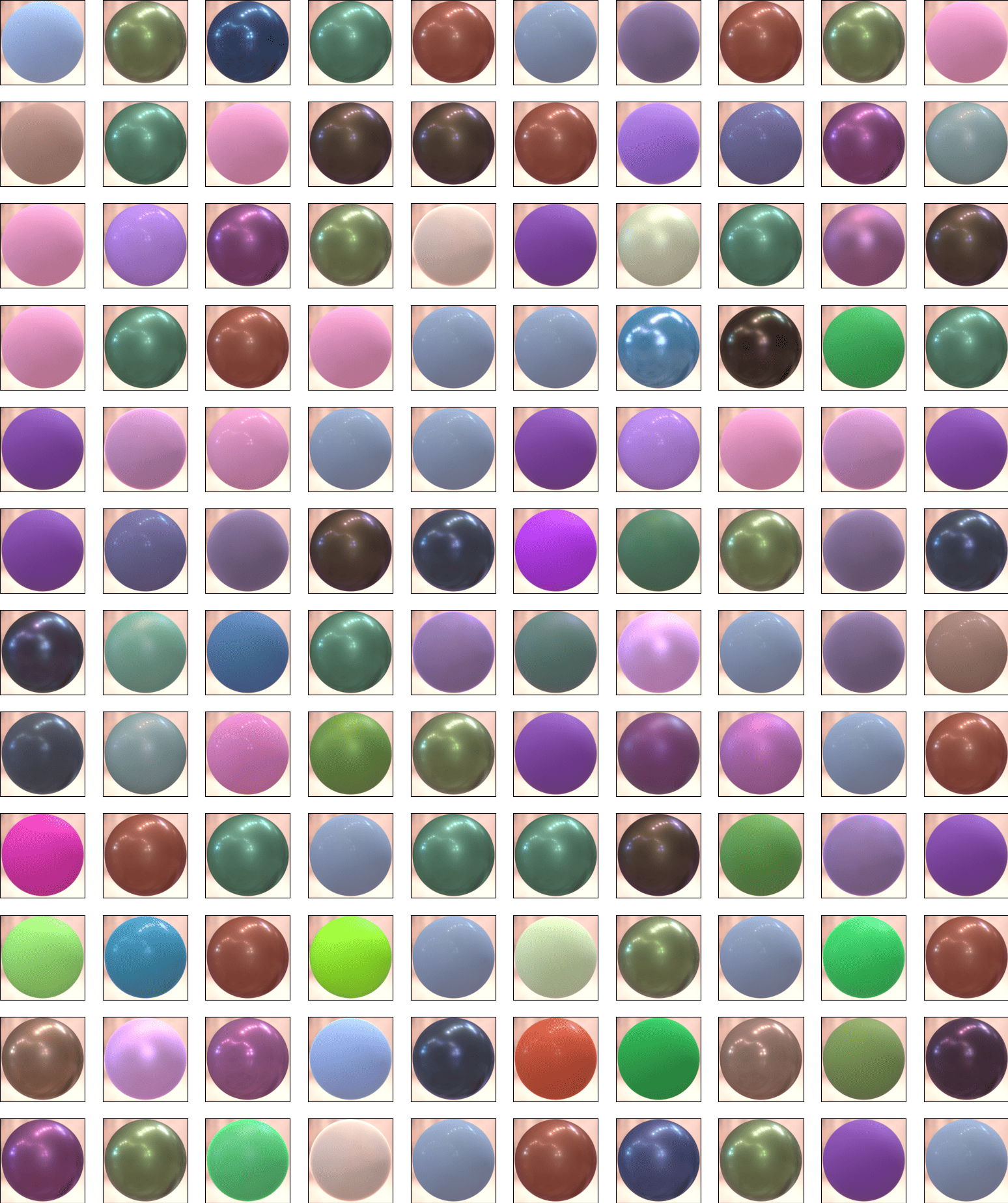
(a) Synthetic set

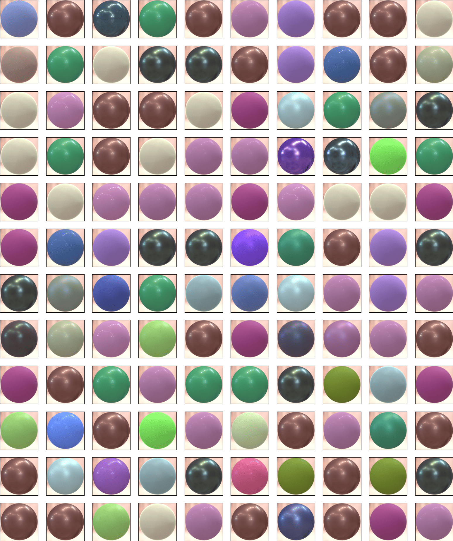
(b) Nearest neighbor reference

Figure 12: Nearest reference under $d_{\text{log}}$ (Eq. 36): for each synthetic material in (a), we identify its nearest neighbor in the refernece set under $d_{\text{log}}$ presented at the same grid position in (b). The nearest neighbor metric is capable of matching most BRDFs in terms of reflective behaviors.

In Fig. 13, we further visualize the nearest neighbor information by plotting the heatmap of pairwise mean squared logarithmic distance defined as

$$d_{\text{MSL}}:=\underset{\theta_{{\bm{\mathbf{h}}}},\theta_{{\bm{\mathbf{d}}}},\varphi_{{\bm{\mathbf{d}}}}}{\mathbb{E}}\Big{[}\left(\log\left(1+f_{r}\cos\theta_{i}\right)-\log\left(1+f_{r}^{\prime}\cos\theta_{i}\right)\right)^{2}\Big{]}.$$ (37)

From the Figure we can see that the nearest neighbor is captured effectively with the underlying distance, validating the design choice of our BRDF distributional metrics.

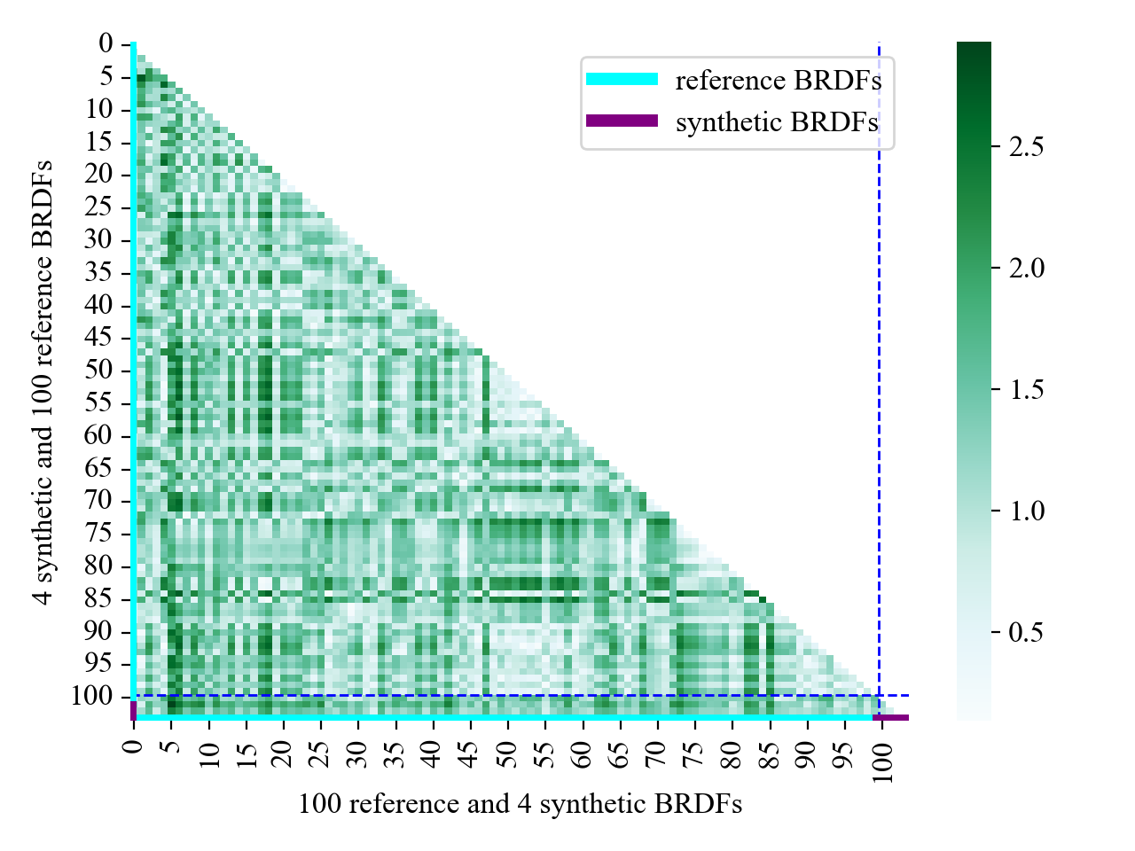
(a) Pairwise distance of synthetic and all reference BRDFs

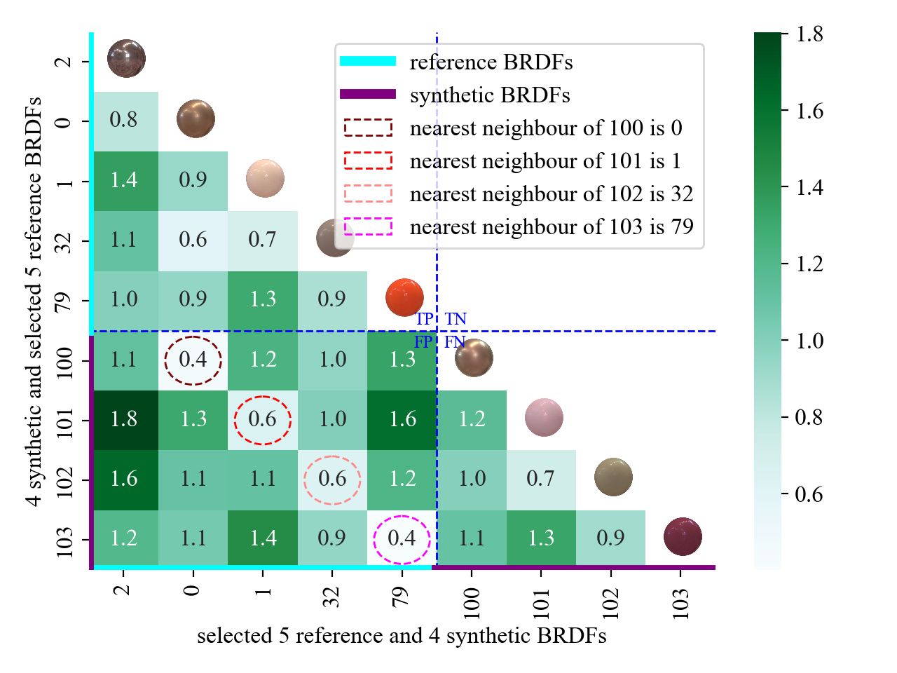
(b) Pairwise distance of synthetic and selected reference BRDFs

Figure 13: Nearest neighbor information illustrated by pairwise mean squared logarithmic distance. We can see that the nearest neighbor is captured effectively with the underlying distance.

E Further Results

E.1 Unconditional Synthesis

For the unconditional synthesis experiment in Sec. 4.3, further results are presented in Figs. 14, 15, 16, 17 and 18 for NeuMaDiff (our method), PCA-A, PCA-N, VAE-A, and VAE-N, respectively

Figure 14: Synthesized materials by NeuMaDiff (our method).

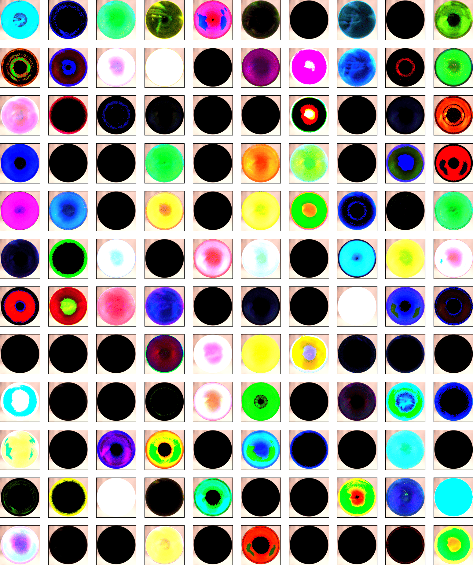
Figure 15: Synthesized materials by PCA-A.

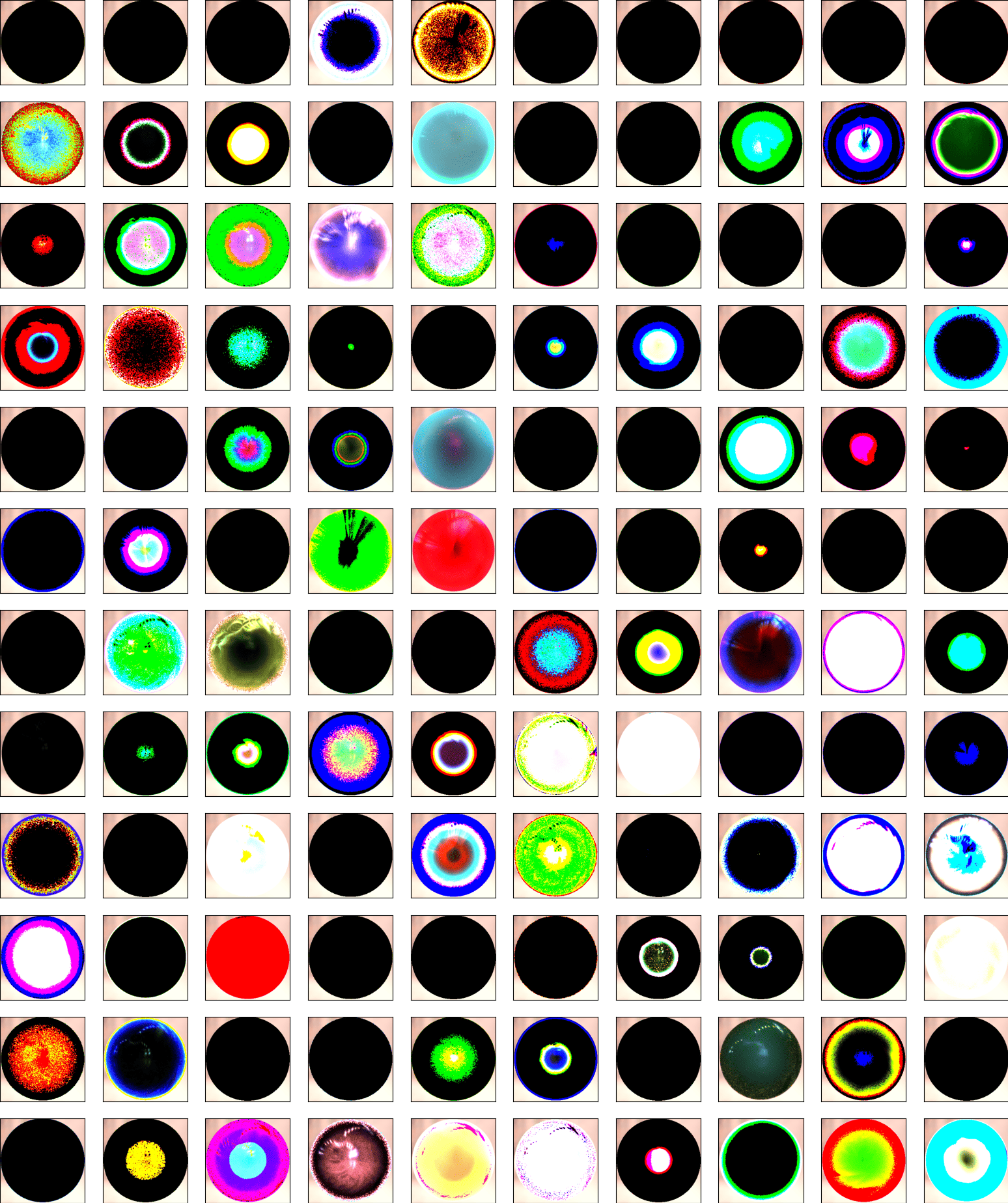
Figure 16: Synthesized materials by PCA-N.

Figure 17: Synthesized materials by VAE-A.

Figure 18: Synthesized materials by VAE-N.

F Additional Experiments

F.1 Statistical Analysis on MERL Dataset

We perform the statistical analysis on the MERL dataset [34]. We collect mean and maximum reflectance values in different color channels across all materials. Figure 19 demonstrates the statistical summary averaged across each material type while Fig. 20 details the statistics in each individual material grouped by type. In addition, to identify the classification boundaries between different material types, in Fig. 21, we apply K-means clustering (for background see Sec. A.5) on the maximum reflectance of red channel.

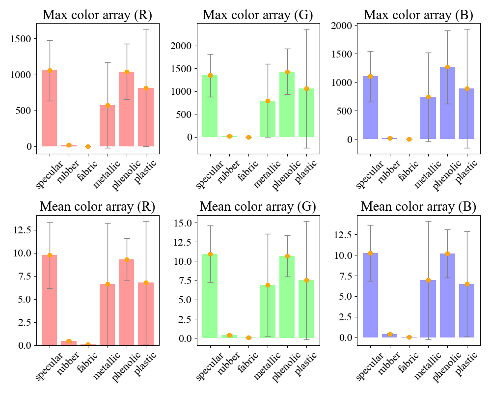
Figure 19: Per-type averaged mean and maximum reflectance.

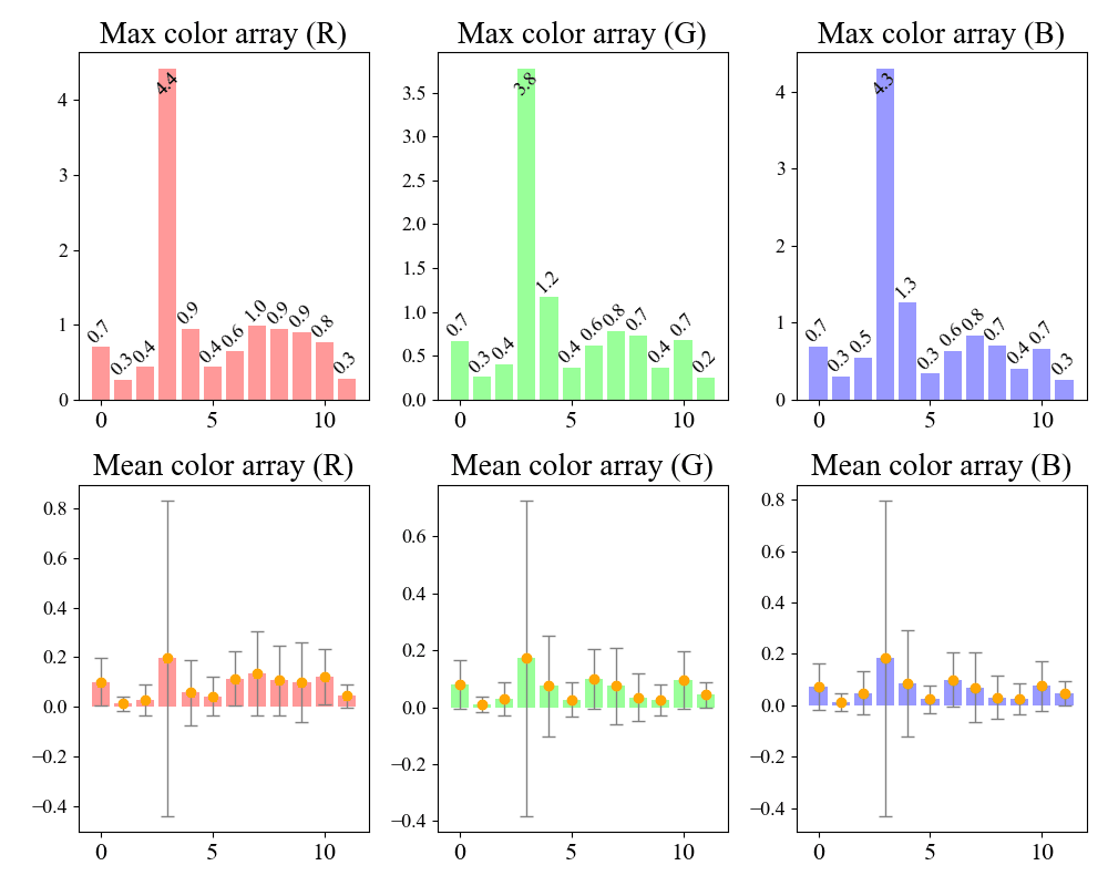
(a) Fabric BRDF statistics

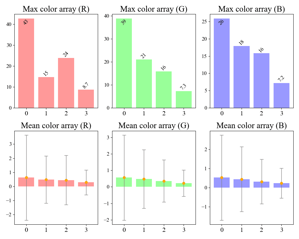
(b) Rubber BRDF statistics

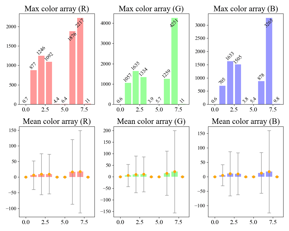
(c) Plastic BRDF statistics

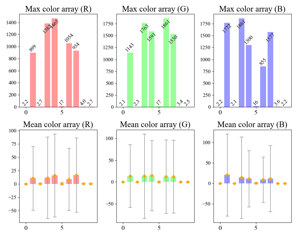
(d) Metallic BRDF statistics

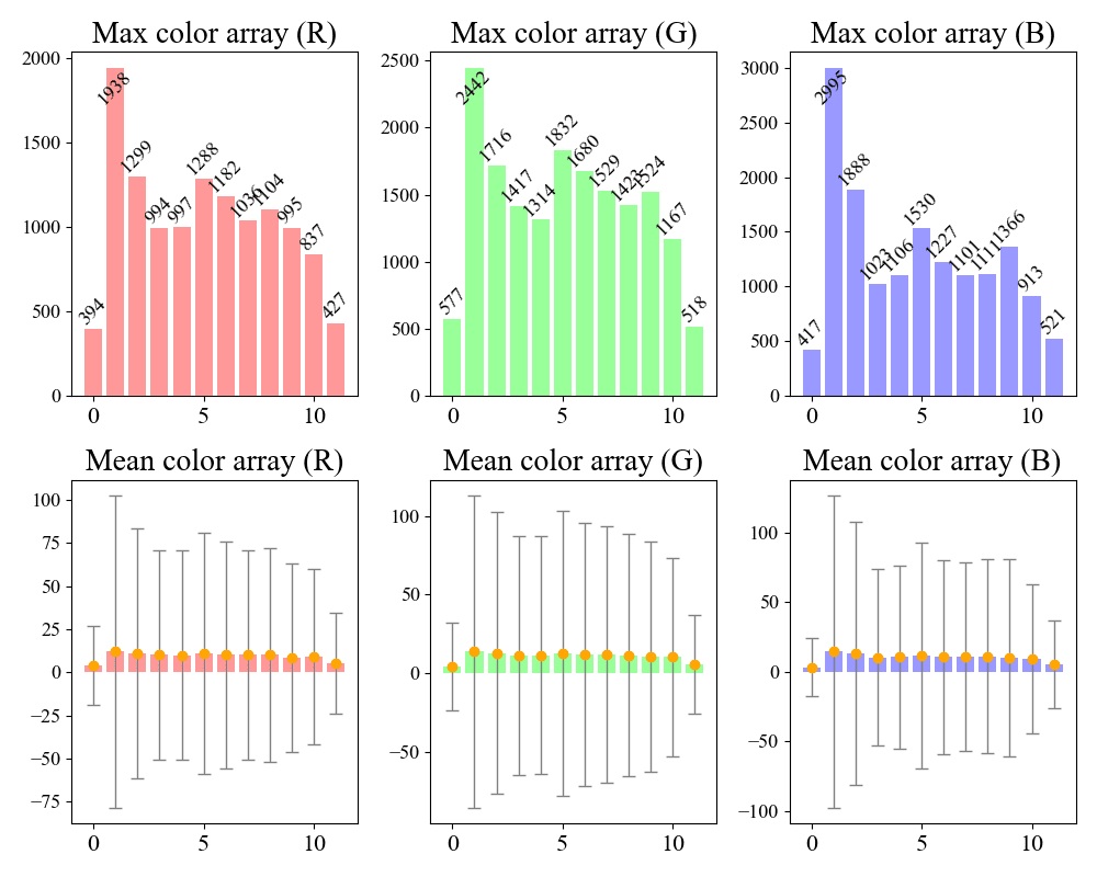
(e) Phenolic BRDF statistics

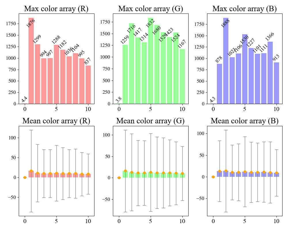
(f) Specular BRDF statistics

Figure 20: Full MERL BRDF [34] statistical analysis grouped by material type.

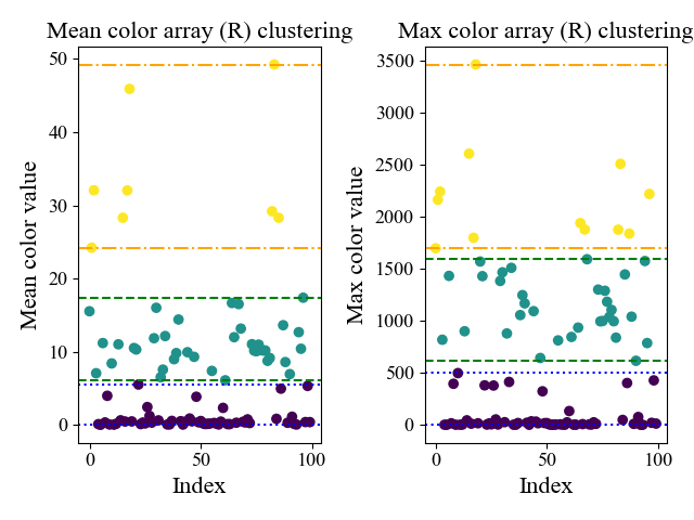
Figure 21: K-means clustering on mean (left) and maximum (right) reflectance of red channel.

F.2 Superresolution for Low-density BRDF

Experiment on the BRDF reconstruction for low-density input, where the position samples density are decreased $x$-time in all three dimension $\theta_{h},\theta_{d},\phi_{d}$ from $90\times 90\times 180$. We take $x=1,2,4,8,16$ as the scaling factor. Given each dimension $x$-time lower density, the number of position samples left are

$$(1+\lfloor\frac{89}{x}\rfloor)\times(1+\lfloor\frac{89}{x}\rfloor)\times(1+\lfloor\frac{179}{x}\rfloor)$$

The reconstruction baseline is to fetch BRDF values taking in position indices, which are rounded down to the nearest neighbor. On the other hand, NBRDF model is trained over low-density data. Under the same scene setting, I measure SSIM of rendered images between full-density ground truth and reconstructed BRDF (Tab. 2). Top results among the two methods are bold.

# samples	$x$	baseline	NBRDF
$90^{2}\times 180$	1x	1 ± 0	0.9987 ± 7e-6
$23^{2}\times 45$	4x	0.996 ± 9.3e-5	0.996 ± 0.00012
$12^{2}\times 23$	8x	0.984 ± 0.001	0.9934 ± 1.475e-4
$6^{2}\times 12$	16x	0.915 ± 0.024	0.962 ± 0.0067
$4^{2}\times 8$	24x	0.823 ± 0.0527	0.896 ± 0.02614
$3^{2}\times 6$	32x	0.745 ± 0.07467	0.831 ± 0.04942

Table 2: Low-density reconstruction comparison (SSIM)

The NBRDF model showcases overwhelming well reconstruction capability over the MERL dataset in all range of position sample densities. This result might be useful in scenario where high-resolution BRDF collection is not available. Moreover, it also lower the entry bar and intensity for BRDF measurement.

References

- Abdi and Williams [2010] Hervé Abdi and Lynne J Williams. Principal component analysis. Wiley interdisciplinary reviews: computational statistics, 2(4):433–459, 2010.
- Achlioptas et al. [2018] Panos Achlioptas, Olga Diamanti, Ioannis Mitliagkas, and Leonidas Guibas. Learning representations and generative models for 3d point clouds. In International conference on machine learning, pages 40–49. PMLR, 2018.
- Bengio and Delalleau [2011] Yoshua Bengio and Olivier Delalleau. On the expressive power of deep architectures. In International conference on algorithmic learning theory, pages 18–36. Springer, 2011.
- Betzalel et al. [2022] Eyal Betzalel, Coby Penso, Aviv Navon, and Ethan Fetaya. A study on the evaluation of generative models, 2022.
- Burley [2012] Brent Burley. Physically-based shading at disney. SIGGRAPH Comput. Graph., 2012.
- Chen et al. [2023a] Dave Zhenyu Chen, Yawar Siddiqui, Hsin-Ying Lee, S. Tulyakov, and Matthias Nießner. Text2tex: Text-driven texture synthesis via diffusion models. 2023 IEEE/CVF International Conference on Computer Vision (ICCV), pages 18512–18522, 2023a.
- Chen et al. [2023b] Rui Chen, Yongwei Chen, Ningxin Jiao, and Kui Jia. Fantasia3d: Disentangling geometry and appearance for high-quality text-to-3d content creation. In Proceedings of the IEEE/CVF International Conference on Computer Vision (ICCV), pages 22246–22256, 2023b.
- Cook and Torrance [1982] R. L. Cook and K. E. Torrance. A reflectance model for computer graphics. ACM Trans. Graph., 1(1):7–24, 1982.
- Csiszár [1975] Imre Csiszár. I-divergence geometry of probability distributions and minimization problems. The annals of probability, pages 146–158, 1975.
- Dana et al. [1999] Kristin J. Dana, Bram van Ginneken, Shree K. Nayar, and Jan J. Koenderink. Reflectance and texture of real-world surfaces. ACM Trans. Graph., 18(1):1–34, 1999.
- Devlin [2018] Jacob Devlin. Bert: Pre-training of deep bidirectional transformers for language understanding. arXiv preprint arXiv:1810.04805, 2018.
- Dupuy and Jakob [2018] Jonathan Dupuy and Wenzel Jakob. An adaptive parameterization for efficient material acquisition and rendering. ACM Transactions on graphics (TOG), 37(6):1–14, 2018.
- Erkoç et al. [2023] Ziya Erkoç, Fangchang Ma, Qi Shan, Matthias Nießner, and Angela Dai. Hyperdiffusion: Generating implicit neural fields with weight-space diffusion. In 2023 IEEE/CVF International Conference on Computer Vision (ICCV), pages 14254–14264, 2023.
- Fan et al. [2022] Jiahui Fan, Beibei Wang, Miloš Hašan, Jian Yang, and Ling-Qi Yan. Neural layered brdfs. In Proceedings of SIGGRAPH 2022, 2022.
- Filip and Vávra [2014] Jirí Filip and Radomír Vávra. Template-based sampling of anisotropic brdfs. In Computer Graphics Forum, pages 91–99. Wiley Online Library, 2014.
- Gatys et al. [2015] Leon Gatys, Alexander S Ecker, and Matthias Bethge. Texture synthesis using convolutional neural networks. Advances in neural information processing systems, 28, 2015.
- Gokbudak et al. [2023] Fazilet Gokbudak, Alejandro Sztrajman, Chenliang Zhou, Fangcheng Zhong, Rafal Mantiuk, and Cengiz Oztireli. Hypernetworks for generalizable brdf estimation. arXiv e-prints, pages arXiv–2311, 2023.
- Guarnera et al. [2016a] D. Guarnera, G.C. Guarnera, A. Ghosh, C. Denk, and M. Glencross. Brdf representation and acquisition. Computer Graphics Forum, 35(2):625–650, 2016a.
- Guarnera et al. [2016b] D. Guarnera, G.C. Guarnera, A. Ghosh, C. Denk, and M. Glencross. Brdf representation and acquisition. Computer Graphics Forum, 35(2):625–650, 2016b.
- Guo et al. [2023] Jie Guo, Zeru Li, Xueyan He, Beibei Wang, Wenbin Li, Yanwen Guo, and Ling-Qi Yan. Metalayer: A meta-learned bsdf model for layered materials. ACM Trans. Graph., 42(6), 2023.
- Haindl and Filip [2013] Michal Haindl and Jiri Filip. Visual texture: Accurate material appearance measurement, representation and modeling. Springer Science & Business Media, 2013.
- He et al. [2016] Kaiming He, Xiangyu Zhang, Shaoqing Ren, and Jian Sun. Deep residual learning for image recognition. In Proceedings of the IEEE conference on computer vision and pattern recognition, pages 770–778, 2016.
- Heusel et al. [2017] Martin Heusel, Hubert Ramsauer, Thomas Unterthiner, Bernhard Nessler, and Sepp Hochreiter. Gans trained by a two time-scale update rule converge to a local nash equilibrium. Advances in neural information processing systems, 30, 2017.
- Ho and Salimans [2022] Jonathan Ho and Tim Salimans. Classifier-free diffusion guidance, 2022.
- Ho et al. [2020] Jonathan Ho, Ajay Jain, and Pieter Abbeel. Denoising diffusion probabilistic models, 2020.
- Hu et al. [2020] Bingyang Hu, Jie Guo, Yanjun Chen, Mengtian Li, and Yanwen Guo. Deepbrdf: A deep representation for manipulating measured brdf. Computer Graphics Forum, 39(2):157–166, 2020.
- Hu et al. [2023] Yiwei Hu, Paul Guerrero, Milos Hasan, Holly Rushmeier, and Valentin Deschaintre. Generating procedural materials from text or image prompts. In ACM SIGGRAPH 2023 Conference Proceedings, pages 1–11, 2023.
- Kingma and Welling [2013] Diederik P Kingma and Max Welling. Auto-encoding variational bayes. arXiv preprint arXiv:1312.6114, 2013.
- Lawrence et al. [2004a] Jason Lawrence, Szymon Rusinkiewicz, and Ravi Ramamoorthi. Efficient brdf importance sampling using a factored representation. In ACM SIGGRAPH 2004 Papers, page 496–505, New York, NY, USA, 2004a. Association for Computing Machinery.
- Lawrence et al. [2004b] Jason Lawrence, Szymon Rusinkiewicz, and Ravi Ramamoorthi. Efficient brdf importance sampling using a factored representation. ACM Transactions on Graphics (ToG), 23(3):496–505, 2004b.
- Li et al. [2006] Hongsong Li, Sing-Choong Foo, Kenneth E. Torrance, and Stephen H. Westin. Automated three-axis gonioreflectometer for computer graphics applications. Optical Engineering, 45(4):043605, 2006.
- Lopez-Paz and Oquab [2016] David Lopez-Paz and Maxime Oquab. Revisiting classifier two-sample tests. arXiv preprint arXiv:1610.06545, 2016.
- Mann et al. [2020] Ben Mann, N Ryder, M Subbiah, J Kaplan, P Dhariwal, A Neelakantan, P Shyam, G Sastry, A Askell, S Agarwal, et al. Language models are few-shot learners. arXiv preprint arXiv:2005.14165, 1, 2020.
- Matusik et al. [2003] W. Matusik, H. Pfister, M. Brand, and L. McMillan. A data-driven reflectance model. ACM Transactions on Graphics (TOG), 22(3):759–769, 2003.
- Memery et al. [2023] Sean Memery, Osmar Cedron, and Kartic Subr. Generating Parametric BRDFs from Natural Language Descriptions . Computer Graphics Forum, 2023.
- Montes and Ureña [2012] Rosana Montes and Carlos Ureña. An overview of brdf models. University of Grenada, Technical Report LSI-2012-001, 2012.
- Nair and Hinton [2010] Vinod Nair and Geoffrey E Hinton. Rectified linear units improve restricted boltzmann machines. In Proceedings of the 27th international conference on machine learning (ICML-10), pages 807–814, 2010.
- Ngan et al. [2005] Addy Ngan, Frédo Durand, and Wojciech Matusik. Experimental analysis of brdf models. Rendering Techniques, 2005(16th):2, 2005.
- Nicodemus et al. [1977] Fred E. Nicodemus, Joseph C. Richmond, Jack J. Hsia, Irving W. Ginsberg, T. Limperis, Sidney Harman, and Jordan J Baruch. Geometrical considerations and nomenclature for reflectance. NATIONAL BUREAU OF STANDARDS, USA, 1977.
- Nielsen et al. [2015] Jannik Boll Nielsen, Henrik Wann Jensen, and Ravi Ramamoorthi. On optimal, minimal brdf sampling for reflectance acquisition. ACM Trans. Graph., 34(6), 2015.
- Peebles et al. [2022] William Peebles, Ilija Radosavovic, Tim Brooks, Alexei A Efros, and Jitendra Malik. Learning to learn with generative models of neural network checkpoints. arXiv preprint arXiv:2209.12892, 2022.
- Phong [1975] Bui Tuong Phong. Illumination for computer generated pictures. Commun. ACM, 18(6):311–317, 1975.
- Radford et al. [2021] Alec Radford, Jong Wook Kim, Chris Hallacy, Aditya Ramesh, Gabriel Goh, Sandhini Agarwal, Girish Sastry, Amanda Askell, Pamela Mishkin, Jack Clark, et al. Learning transferable visual models from natural language supervision. In International conference on machine learning, pages 8748–8763. PMLR, 2021.
- Romeiro and Zickler [2010] Fabiano Romeiro and Todd Zickler. Blind reflectometry. In Computer Vision–ECCV 2010: 11th European Conference on Computer Vision, Heraklion, Crete, Greece, September 5-11, 2010, Proceedings, Part I 11, pages 45–58. Springer, 2010.
- Rusinkiewicz [1998] Szymon Rusinkiewicz. A new change of variables for efficient BRDF representation. In Eurographics Workshop on Rendering, Vienna, Austria, 1998.
- Serrano et al. [2016] Ana Serrano, Diego Gutierrez, Karol Myszkowski, Hans-Peter Seidel, and Belen Masia. An intuitive control space for material appearance. SIGGRAPH ASIA, 35(6):186:1–186:12, 2016.
- Song et al. [2021] Jiaming Song, Chenlin Meng, and Stefano Ermon. Denoising diffusion implicit models. ICLR 2021, 2021.
- Sun et al. [2018] Tiancheng Sun, Henrik Wann Jensen, and Ravi Ramamoorthi. Connecting measured brdfs to analytic brdfs by data-driven diffuse-specular separation. ACM Transactions on Graphics (TOG), 37(6):1–15, 2018.
- Sztrajman et al. [2021] Alejandro Sztrajman, Gilles Rainer, Tobias Ritschel, and Tim Weyrich. Neural brdf representation and importance sampling. Computer Graphics Forum, 2021.
- Tchapmi et al. [2022] Lyne P Tchapmi, Trishiet Ray, Micael Tchapmi, Bokui Shen, Roberto Martin-Martin, and Silvio Savarese. Generating procedural 3d materials from images using neural networks. In Proceedings of the 2022 4th International Conference on Image, Video and Signal Processing, pages 32–40, 2022.
- Theis et al. [2016] Lucas Theis, Aäron van den Oord, and Matthias Bethge. A note on the evaluation of generative models, 2016.
- Vaswani [2017] A Vaswani. Attention is all you need. Advances in Neural Information Processing Systems, 2017.
- Walter et al. [2007] Bruce Walter, Stephen R. Marschner, Hongsong Li, and Kenneth E. Torrance. Microfacet models for refraction through rough surfaces. In Proceedings of the 18th Eurographics Conference on Rendering Techniques, page 195–206, Goslar, DEU, 2007. Eurographics Association.
- Wang et al. [2004] Zhou Wang, A.C. Bovik, H.R. Sheikh, and E.P. Simoncelli. Image quality assessment: from error visibility to structural similarity. IEEE Transactions on Image Processing, 13(4):600–612, 2004.
- Weinmann and Klein [2015] Michael Weinmann and Reinhard Klein. Advances in geometry and reflectance acquisition (course notes). In SIGGRAPH Asia 2015 Courses, New York, NY, USA, 2015. Association for Computing Machinery.
- Weinmann et al. [2014] Michael Weinmann, Juergen Gall, and Reinhard Klein. Material Classification Based on Training Data Synthesized Using a BTF Database. In Computer Vision - ECCV 2014 - 13th European Conference, Zurich, Switzerland, September 6-12, 2014, Proceedings, Part III, pages 156–171. Springer International Publishing, 2014.
- Westin et al. [2004] Stephen H Westin, Hongsong Li, and Kenneth E Torrance. A comparison of four brdf models. In Eurographics Symposium on Rendering, pages 1–10, 2004.
- White et al. [1998] D. Rod White, Peter Saunders, Stuart J. Bonsey, John van de Ven, and Hamish Edgar. Reflectometer for measuring the bidirectional reflectance of rough surfaces. Appl. Opt., 37(16):3450–3454, 1998.
- Yang et al. [2019] Guandao Yang, Xun Huang, Zekun Hao, Ming-Yu Liu, Serge Belongie, and Bharath Hariharan. Pointflow: 3d point cloud generation with continuous normalizing flows. In Proceedings of the IEEE/CVF international conference on computer vision, pages 4541–4550, 2019.
- Zhang et al. [2024] Shangzhan Zhang, Sida Peng, Tao Xu, Yuanbo Yang, Tianrun Chen, Nan Xue, Yujun Shen, Hujun Bao, Ruizhen Hu, and Xiaowei Zhou. Mapa: Text-driven photorealistic material painting for 3d shapes, 2024.
- Zheng et al. [2021] Chuankun Zheng, Ruzhang Zheng, Rui Wang, Shuang Zhao, and Hujun Bao. A compact representation of measured brdfs using neural processes. ACM Trans. Graph., 41(2), 2021.
- Zhou et al. [2023] Chenliang Zhou, Fangcheng Zhong, and Cengiz Oztireli. Clip-pae: Projection-augmentation embedding to extract relevant features for a disentangled, interpretable and controllable text-guided face manipulation. In Proceedings of ACM SIGGRAPH 2023, pages 1–9, 2023.
- Zhou et al. [2024] Chenliang Zhou, Alejandro Sztrajman, Gilles Rainer, Fangcheng Zhong, Fazilet Gokbudak, Zhilin Guo, Weihao Xia, Rafal Mantiuk, and Cengiz Oztireli. Physically based neural bidirectional reflectance distribution function, 2024.
- Zhou et al. [2018] Yang Zhou, Zhen Zhu, Xiang Bai, Dani Lischinski, Daniel Cohen-Or, and Hui Huang. Non-stationary texture synthesis by adversarial expansion. arXiv preprint arXiv:1805.04487, 2018.