Pricing Weather Derivatives: A Time Series Neural Network Approach
Abstract.
The objective of the paper is to price weather derivative contracts based on temperature and precipitation as underlying climate variables. We use a neural network approach combined with time series forecast to value Pacific Rim index in Toronto and Chicago
Key words and phrases:
weather derivatives, ARIMA models, machine learning, Pacific Rim1. Introduction
In this paper we analyze the pricing of weather derivative contracts(WD) based on temperatures and precipitation as underlying climate variables. We consider a payoff that is a function of the Pacific Rim Index, defined as the average daily temperatures and precipitation over certain period.
Different approaches for the pricing have been considered in the past. A Historic Burn Approach(HBA), based on the historic behavior of the contract’s payoff, valuations considering the empirical probability density function (p.d.f.) of the index and the dynamic of the underlying climatic variable combined with a Fourier inversion have been previously considered among others. An account on weather derivatives contracts can be found in [1, 8].
In this paper we follow an actuarial approach based on the discounted expected losses of the contract under the historic measure. For a methodology of pricing WD under a risk-neutral framework via an Esscher transform see [9] and references within.
Moreover, our valuation of WD contracts based on temperatures relies on the temperature forecast over the contract’s life expand, leading to predictions of the corresponding payoff. The temperature values are predicted by means of a classic time series model in the class of Autoregressive Moving Average models (ARMA), combined with a harmonic least squares regression and, alternatively, following a neural network approach.
The forecasting of a time series using neural networks and machine learning has been less explored. See for example [2, 11]. Classic ARIMA forecasting is standard, see for example [5, 10]. In connection with the pricing of WD, see time series classic approaches in [3, 4].
For a precipitation WD contract, also based on a Pacific Rim index, we assume that the accumulated precipitation over the period is a random sum of Gamma distributed and independent random variables representing the daily precipitations, while the number of rainy days has a Poisson distribution.
Both the time series and neural network approaches are implemented to temperatures and precipitation in the cities of Chicago and Toronto.
The organization of the paper is the following:
In section 2 we fit a harmonic regression and an ARMA model to temperature data in Toronto and Chicago and forecast the values for the month of December 2023.
In section 3 we discuss the forecast of temperature using a neural network approach.
In section 4 we fit the precipitation model using maximum likelihood and neural network technique, while in section 5 we show the pricing of the contract using direct time series forecast and neural network approaches. Finally, in section 6 we present the conclusions.
2. Forecasting temperatures: A time series approach
Let be a sequence of random variables representing the temperature at certain region on day . Typically, daily temperature data consist of an average of the maximum and the minimum values during the day. We notice the presence of a seasonal component as empirical data show.
The first model for temperature combines a harmonic regression with an ARMA(2,3) model. We also investigated the addition of a GARCH(1,1) model, however the latter does not show any improvement in the fitting.
The forecast for daily temperature is done for the month of December 2023.
The data have been obtained from the NASA Earth Science/Applied Science Program (website:https://power.larc.nasa.gov). Observations are recorded through satellite. They could be less accurate as measuring temperature data from satellites requires statistical models to process the data gathered. The time period covered by the data ranges from 01/01/1981- 12/31/2023. Specific locations in Toronto and Chicago data collection are shown in Table 1.
| Location | Lat. | Long. |
|---|---|---|
| Toronto | 43.6523 | -79.3839 |
| Chicago | 41.4047 | -89.6420 |
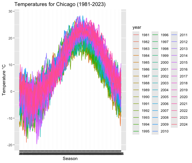
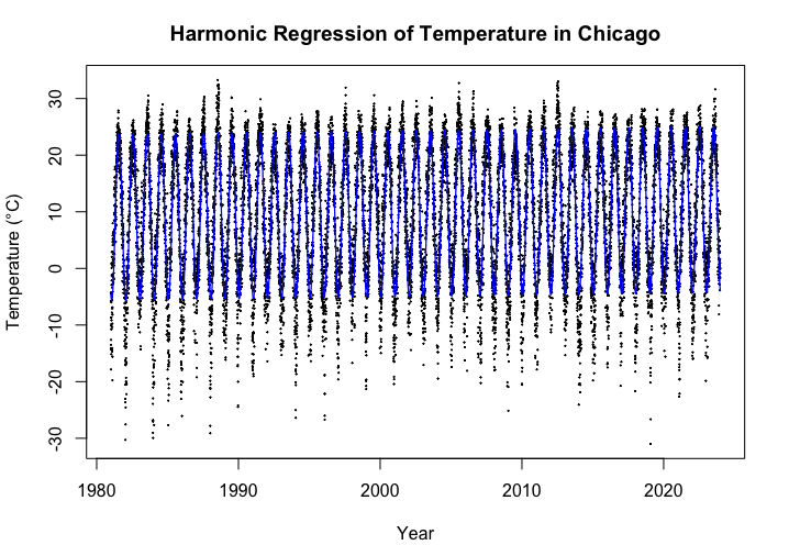
In figures 1(a) and 1(b) the values of temperatures in Toronto and Chicago cities, measured in Celsius degrees, are respectively shown. Each curve represents a particular year. Seasonal effects of temperatures on both cities can be observed. However, seasonality is less clearly seen in the graph for precipitation.
Table 2 complement the information with some statistics of the temperature and precipitation data.
Notice that the negative value of the kurtosis in temperatures indicates the presence of tails lighter than those of the normal distribution, while the precipitation exhibits a large kurtosis in both cities, even larger in Chicago. Also, the data is right skewed. The average number of rainy days in December for Toronto and Chicago are respectively and .
| Location | Minimum | Maximum | Mean | Std Dev | Skewness | Kurtosis |
| Toronto Temp. | -19.7 | 28.35 | 8.37017 | 9.254303 | -0.053197 | -0.949363 |
| Toronto precip. | 0.01 | 41.59 | 2.04 | 3.34 | 3.36 | 16.11 |
| Chicago Temp. | -31 | 33.28 | 9.690668 | 11.42069 | -0.3264819 | -0.777556 |
| Chicago precip. | 0.01 | 75.93 | 3.47 | 6.41 | 3.59 | 19 |

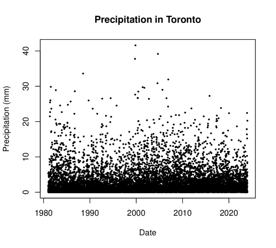
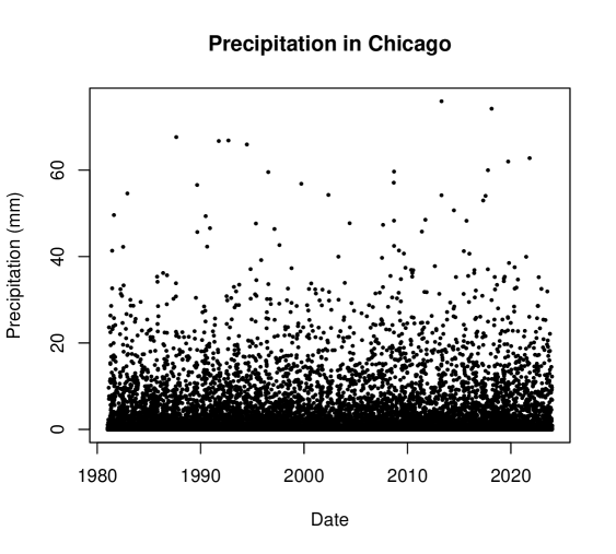
In Figures 2(a) and 2(b) daily precipitation data in Toronto and Chicago from 1981-2023 are respectively shown.
Results about the fitting a harmonic regression to data are given in the Table 3. Notice that all coefficients are significantly different from zero, as reflected in the p-value.
| Toronto | ||||
|---|---|---|---|---|
| Parameter | Estimate | SE | t-Stat | p-Value |
| 6.904 | 6.613e-02 | 104.39 | <2e-16 | |
| 8.665e-05 | 7.482e-06 | 11.58 | <2e-16 | |
| -6.809 | 4.673e-02 | -145.69 | <2e-16 | |
| -1.244e+01 | 4.679e-02 | -265.90 | <2e-16 | |
| Chicago | ||||
| Parameter | Estimate | SE | t-Stat | p-Value |
| 6.904 | 6.613e-02 | 104.39 | <2e-16 | |
| 8.665e-05 | 7.482e-06 | 11.58 | <2e-16 | |
| -6.809e+00 | 4.673e-02 | -145.69 | <2e-16 | |
| -1.244e+01 | 4.679e-02 | -265.90 | <2e-16 |
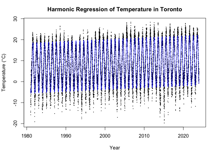
In figures 3(a) and 3(b) harmonic regression fit for daily temperature time-series in Toronto and Chicago are represented. The blue curve represents the regression and the black dots are the actual temperatures. On the other hand, figures 4(a) and 4(b) show the residual values in both fittings. It can be appreciated that the residuals from the harmonic regression do not resemble white noise. By performing an Augmented Dicky-Fuller test on the residuals we see that they are stationary. This fact suggests an ARIMA model can be used for the residuals. The top figure shows the scatter plot for the residuals of the harmonic regression and the bottom shows the density plot of these residuals compared with the density plot of the normal distribution.
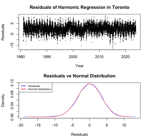
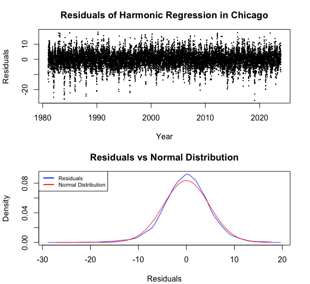
A Kolmogorov-Smirnov test for the temperature data in both cities rejects t-student, stable and inverse Gaussian distributions. In both cases the test fails to reject the normality. On the other hand, auto-correlation and partial auto-correlation in the residuals could be observed.
The values and in the ARMA model are selected to minimize the Akaike information criterion (AIC) and Bayesian information criterion (BIC). We conducted testing on models with autoregressive(AR) and moving average (MA) components up to order five. The optimal values of the order according to the Akaike criterion are and for both, Toronto and Chicago cities.
We also look at the largest significant lags in the autocorrelation (ACF) and partial autocorrelation (PACF) functions to further justify the choice of an ARMA(2,3) model. The ACF of the residuals contains several statistically significant lags. From the PACF function we see that there are two major spikes, as such we should expect the ARMA model to have an autoregressive component of two our model by observation be ARMA(p=2, q=3).
The estimation of the coefficients is done by a maximum likelihood approach. Their values and their corresponding standard errors can be seen in Table 4.
| Toronto | |||||
|---|---|---|---|---|---|
| Estimate | 1.5426 | -0.5511 | -0.7387 | -0.2842 | 0.0947 |
| S.E | 0.0357 | 0.0343 | 0.0375 | 0.0120 | 0.0213 |
| Chicago | |||||
| Estimate | 1.5256 | -0.5475 | -0.6036 | -0.3226 | 0.0443 |
| S.E | 0.0384 | 0.0332 | 0.0396 | 0.0097 | 0.0173 |
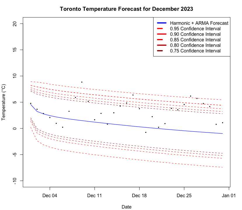
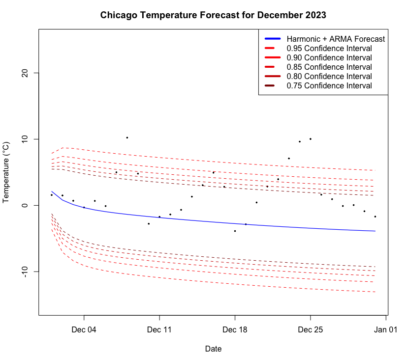
In Figures 5(a) and 5(b) the forecast of temperatures for the month of December 2023 are shown. The blue curve at the center is the daily forecast with the red curves are the confidence limits with confidence levels ranging from 75% and 95%.
The time series analysis has been carried out using R studio.
3. Forecasting temperatures: A neural network approach
We consider a neural network to train and forecast temperature data. We will benchmark this neural network model to two more traditional models considered in the previous section.
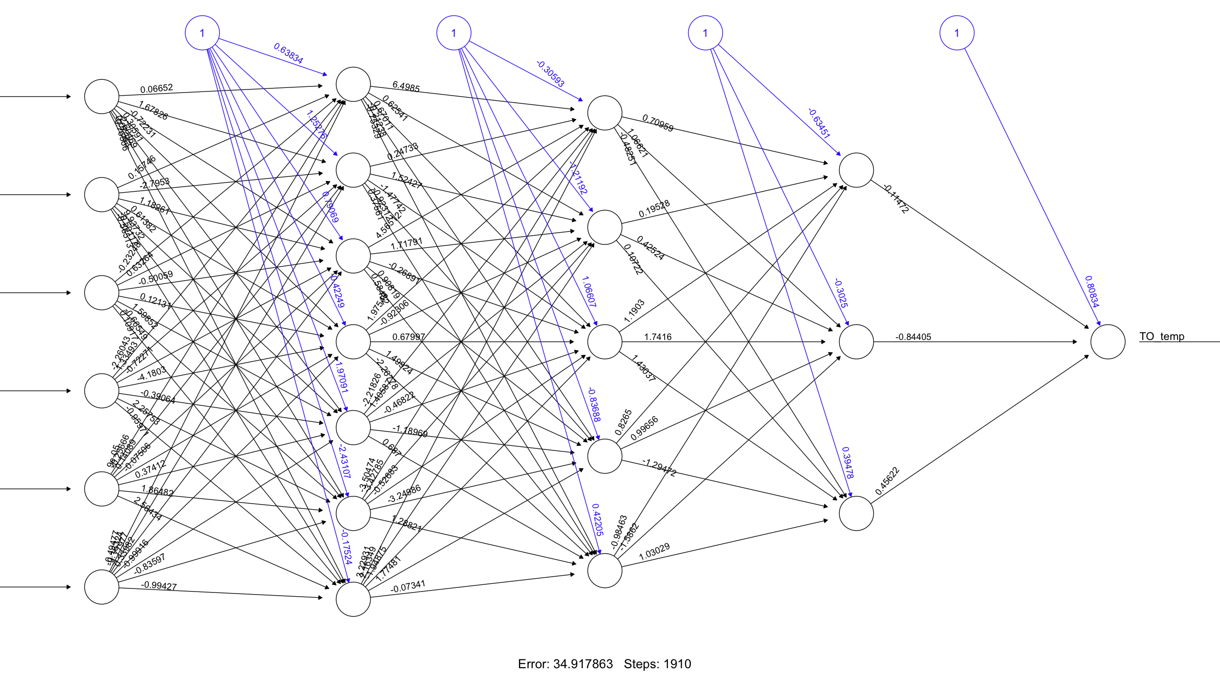
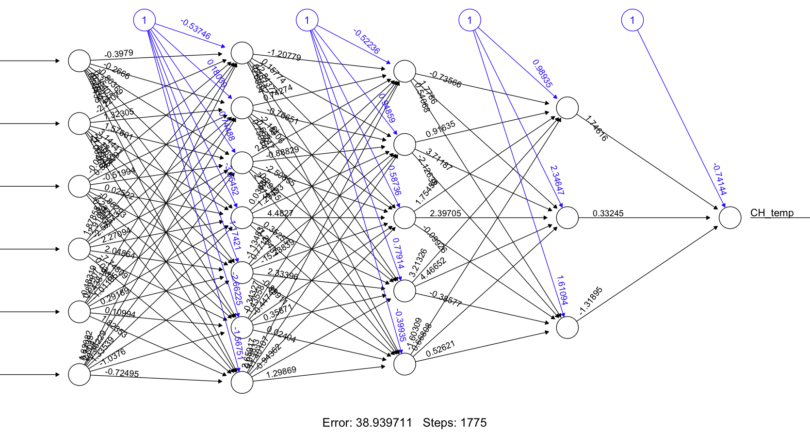
The neural networks into consideration have three hidden layers with (7,5,3) neurons in each layer. It is important to note that this is the largest neural network we are able to train on the system using R Studio.
The six inputs we use in the neural network for Toronto and Chicago are the following: year, month, day, temperature one year ago, temperature two years ago, and the data from the harmonic regression. To keep the dimensional of the data low, we chose to encode year, month, and day data using label encoding.
We chose this method of encoding categorical variables for two main reasons.
First, year, month, and day have a natural chronological order. Second, we want to keep the dimensionality of the data to be low. It is important to note that one-hot encoding might be a better choice to represent the data, but at the expense of increased dimensionality. The use of this encoding is common in machine learning when categorical data needs to be represented numerically, see [5, ML_python].
We also use the temperature of the previous two years as an input to the network because the harmonic regression is not able to model all the seasonality present in the data. By adding the values of the harmonic regression and the previous two years of daily average temperature as inputs we intend a better capture these seasonal dynamics.
Because we take the temperature from two years ago as an input, the neural network is trained on the remaining 40 years of historical data. We apply min-max normalization on the features and log-normalization on target variable (DAT).
This normalization is done in order to speed up the training time, and the convergence of our model, see [6]. A Resistant Back Propagation Algorithm is used to find the weights in the models.
We arrive at the architecture exposed above by measuring the Mean Square Error (MSE) of different neural networks on a validation set that is withheld from the training and testing sets. Neural networks up to three hidden layers and ten neurons per layer were tested. Using a validation set to find the best architecture for a neural network is best practice. Performing this testing on the testing set could lead to data-leakage and an over fit model. See [7]. While the number of neurons is the same in the neural network that forecasts temperature in Chicago and Toronto, all the weights in each neural network are different because each neural network was trained on a different set of data. A visualization of the neural network can be seen in Figure 6.
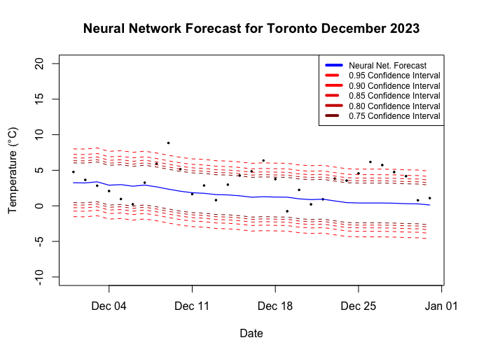
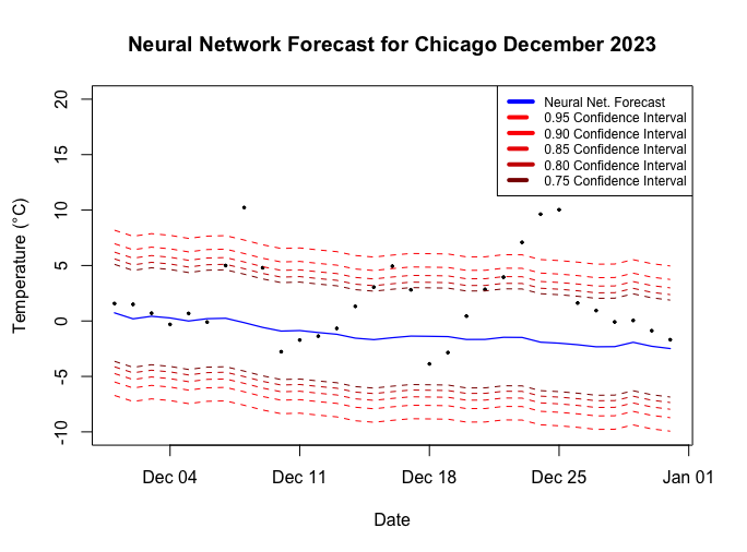
The forecast of the temperatures for Toronto in December 2023 can be seen in Figure 7. We can see that both forecasts still underestimate the temperature for December 2023. There are multiple values in our forecast that pass the upper 95 % confidence interval. A major reason of this underestimation is that this particular month in 2023 was unusually hot when compared to other months in December during past years.
In Figure 8 we can see the p.d.f. plot of average temperatures in December from 1981-2023. In this graph the red lines represent the 0.95 confidence interval for temperature in December and the blue line represents the observed temperature in December 2023. From the graph we can see that December 2023 seems an outlier month with unusually high temperatures.
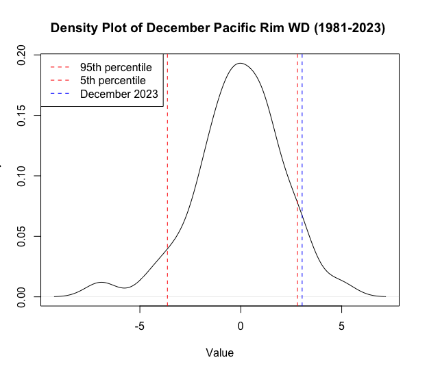
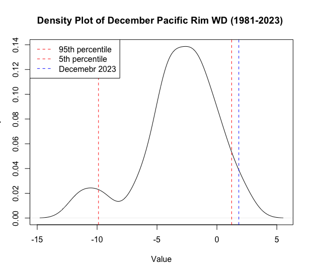
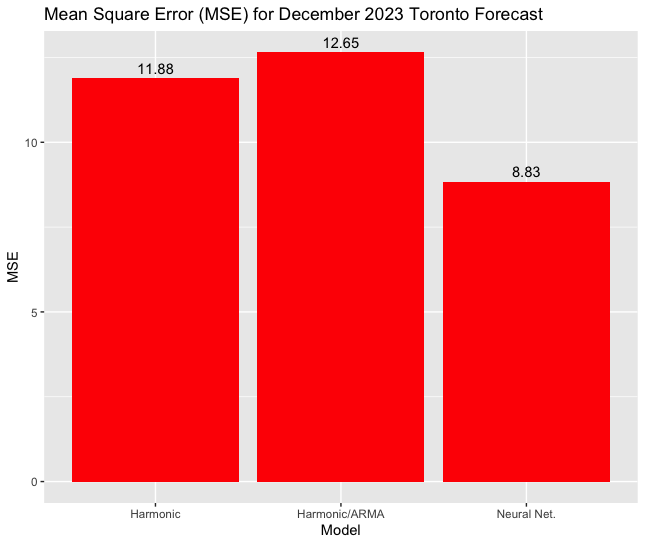
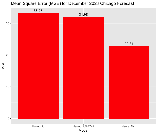
The underestimation, due to unusually high temperatures for December 2023 is also present in the Chicago forecast. As can be seen in the p.d.f. plot for average temperature in December in Figure 8, the average temperature for December 2023 seems to be an outlier month. One of the possible reasons for these usually high temperatures in 2023 was is the presence of the El Niño phenomenon. We believe that the neural network model provides a better prediction than the Harmonic and Harmonic/ARMA models because the former is better able to handle the non-linear patterns in the data. The ARMA model assumes linear relationships in the data which might not be a good assumption when dealing with DAT data. The neural network can identify crucial patterns in raw data with less manual feature engineering which saves time and effort. On the other hand over engineering the input data into a neural network model could lead to poor forecasts. The MSE for the harmonic regression, harmonic regression plus an ARMA model, and the neural network for Toronto and Chicago, December 2023 forecasts are shown in Figure 9. It can be noticed that the MSE is smaller when a neural network approach is considered, compared with the one based on a harmonic regression model and a harmonic model combined with an ARMA(2,3) model.
4. Precipitation model and estimation analysis
In modeling precipitation let be the random number of rainy days within the lifespan of the contract and the amount of precipitation on the k-th day with non-zero precipitation. Thus, the average precipitation during the lifespan of the contract is given by :
| (1) |
Furthermore, we assume that the random variable has a Poisson distribution with parameter , independent of the daily amount of precipitation.
Moreover, the daily precipitation amounts are suppose to be independent with a Gamma distribution with parameters . It p.d.f. is:
We estimate the parameters and using maximum likelihood estimation (MLE) and convolutional neural network (CNN) approaches.
We also test the hypothesis that the distribution of the daily total precipitation (DTP) over the course of a year changes with respect to the season. To this end, we estimate the parameters for each season (summer, winter, spring and fall) and for the entire year. We also calculated the confidence interval of the estimates. See tables 5 and 6.
From Table 5 we can see that the and parameters differ between seasons, specifically in the winter season. We chose to train it using data from only the winter months.
Our CNN is trained on generated data from gamma distribution with different parameters. To train the CNN the parameters are the target variables. The generated values serve as the input set. This method for estimating parameters assumes that the testing data is represented somewhere within the generated training data. Our training set covers the parameters in the range of 0.01 to 5 units. We select this range based on the estimates provided through the
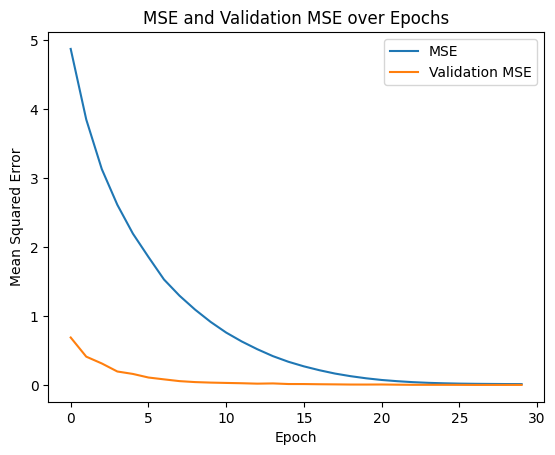
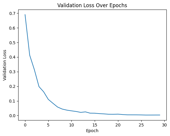
MLE method. The training and validation loss functions of the CNN can be observed in figures 10(a) and 10(b). From these figures we can see that the validation loss tapered off after epoch 25. We can confirm that we did not over-train the model as there is no increase in validation loss as the MSE decreased. We attribute the fact that the validation loss is lower than the MSE to the fact that we use generated data to train the model.
If we would like to see if the Gamma distribution with the parameters estimated are representative of the precipitation data we could see if they can be used to estimate the four moments of the precipitation data.
| Season | ||||||
|---|---|---|---|---|---|---|
| Toronto | 0.516 | 0.253 | 0.0050 | 0.0038 | [0.506, 0.526] | [0.245, 0.260] |
| Toronto Summer | 0.516 | 0.220 | 0.0101 | 0.0067 | [0.497, 0.536] | [0.207, 0.233] |
| Toronto Winter | 0.580 | 0.377 | 0.0113 | 0.0110 | [0.558, 0.602] | [0.356, 0.399] |
| Toronto Spring | 0.493 | 0.245 | 0.0096 | 0.0075 | [0.474, 0.512] | [0.230, 0.260] |
| Toronto Fall | 0.504 | 0.221 | 0.0098 | 0.0067 | [0.484, 0.523] | [0.208, 0.235] |
| Chicago | 0.371 | 0.107 | 0.0039 | 0.0020 | [0.363, 0.378] | [0.103, 0.110] |
| Chicago Summer | 0.413 | 0.097 | 0.0084 | 0.0034 | [0.397, 0.430] | [0.091, 0.104] |
| Chicago Winter | 0.354 | 0.166 | 0.0076 | 0.0064 | [0.339, 0.369] | [0.154, 0.179] |
| Chicago Spring | 0.391 | 0.104 | 0.0082 | 0.0037 | [0.375, 0.407] | [0.097, 0.111] |
| Chicago Fall | 0.349 | 0.096 | 0.0076 | 0.0037 | [0.334, 0.364] | [0.088, 0.103] |
Details in the architecture of the CNN are given below:
| CNN Architecture | ||||
| Conv2D Layer: | ||||
| BatchNormalization Layer | ||||
| MaxPooling2D Layer: | Default pool size | |||
| Conv2D Layer: | ||||
| BatchNormalization Layer | ||||
| MaxPooling2D Layer: | Default pool size | |||
| Flatten Layer | ||||
| Dense Layer: | ||||
| BatchNormalization Layer | ||||
| Dropout Layer: | ||||
| Dense Layer: | ||||
| BatchNormalization Layer | ||||
| Dropout Layer: | ||||
| Dense Layer: | 2 units (output layer for predicting alpha and beta) | |||
| Season | ||||||
|---|---|---|---|---|---|---|
| Toronto | 0.45 | 0.45 | 0.0215 | 0.0207 | [0.41, 0.49] | [0.41, 0.49] |
| Toronto Summer | 0.43 | 0.43 | 0.0236 | 0.0224 | [0.38, 0.48] | [0.39, 0.48] |
| Toronto Winter | 0.48 | 0.49 | 0.0260 | 0.0254 | [0.43, 0.53] | [0.44, 0.54] |
| Toronto Spring | 0.31 | 0.37 | 0.0202 | 0.0191 | [0.27, 0.35] | [0.33, 0.41] |
| Toronto Fall | 0.41 | 0.42 | 0.0389 | 0.0330 | [0.33, 0.49] | [0.36, 0.48] |
| Chicago | 0.18 | 0.16 | 0.0376 | 0.0334 | [0.11, 0.25] | [0.10, 0.23] |
| Chicago Summer | 1.46 | 1.71 | 0.0322 | 0.0275 | [1.40, 1.52] | [1.66, 1.76] |
| Chicago Winter | 0.23 | 0.22 | 0.0289 | 0.0313 | [0.17, 0.29] | [0.16, 0.28] |
| Chicago Spring | 0.66 | 0.65 | 0.0248 | 0.0268 | [0.61, 0.71] | [0.60, 0.70] |
| Chicago Fall | 0.03 | 0.01 | 0.0254 | 0.0270 | [-0.02, 0.08] | [-0.04, 0.06] |
5. Weather derivatives: pricing results
Most weather derivative contracts are based on accumulated temperatures or precipitations (CAT), heating-degrees-days (HDD) or cooling-degrees-days (CDD) over certain period containing days. A Pacific Rim index considers the average value of the climate underlying variable. The later is defined, respectively for temperature and precipitation, as:
| (2) | |||||
| (3) |
In days with no precipitation .
The payoff for these contracts are represented by a strangle contract, i.e. a European long put and long call with different strikes. In this formula and represent the dollar amount paid per degree above or below the strike prices and respectively. This comes to $20 for
contracts in Fahrenheit degrees, and $36 for contracts in Celsius degrees. Similar interpretation stands for and .
The price of WD contracts based on temperatures and precipitation are then given by:
| (4) | |||||
| (5) |
where
| (6) | |||||
| (7) |
and and are the respective p.d.f.’s of the Pacific Rim indices for temperatures and precipitation.
As pricing reference we use the Historic Burn approach(HBA), see [11]. Despite of its inaccuracies HBA remains rather popular between practitioners. It consists in looking at past payoffs of the contract and compute their mean value conveniently discounted. A linear trend might be removed form the data to account for non-stationarity due to local change in urbanization or global warming. A premium is added to account for the risk of writing the contract, as much as 20%-25% of its standard deviation in practice. In summary the price using HBA can be written as:
where is the value of the payoff on the k-th year, is its standard deviation and is the number of years back in the analysis. Here is the Pacific Rim index for temperature or precipitation.
The estimated payoff for the temperature contract is calculated based on the forecasts of the Harmonic/ARMA(2,3) and the neural network model. Alternatively, a forecast for the Pacific Rim index can be estimated through Monte Carlo simulations of a gamma distribution that estimates precipitation for precipitation days.
For the numerical study we carry on, the strike prices are selected as the percentiles of temperature and precipitation. The level of the percentile ranges on the interval .
5.1. Pricing Toronto and Chicago temperatures
In Table 7 we can see the forecast for the Pacific Rim index for Toronto and Chicago in December 2023. The first line represents the value for the Pacific Rim index across the data time expand, while the second line shows the 40 year average of the index only for December from 1982 to 2022. The next three following lines represents the index forecast under the harmonic regression, the harmonic regression/ARMA and the one using neural networks.
The results indicate that neural networks are more capable at predicting daily average temperature when the forecast window is one month. Using the forecasts from the Harmonic/ARMA model and the neural network model we calculate the the estimated payoff for a strangle contract for different strike prices.
Confidence intervals in the forecasts for December for the harmonic/ARMA and neural network model can be seen in figures 5 and 7. We observe that the payoff of the WD strangle contract is larger for more extreme weather forecasts. The largest estimated payouts occur when we expect much lower temperatures, or much higher temperatures. This is why the values in the further bounds of the confidence intervals of the weather forecast correspond to higher estimated payoffs. However, the payoffs are less likely to be observed, as they do not represent the most likely outcome.
Having both a call and put option allows for a payoff when temperatures are either higher or lower. This makes a strangle contract a favorable contract to hold when temperatures could be much higher or lower than expected.
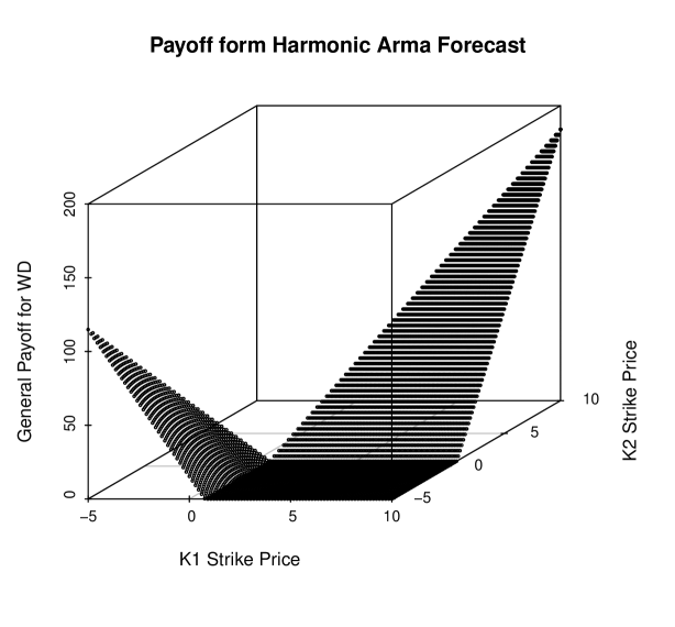
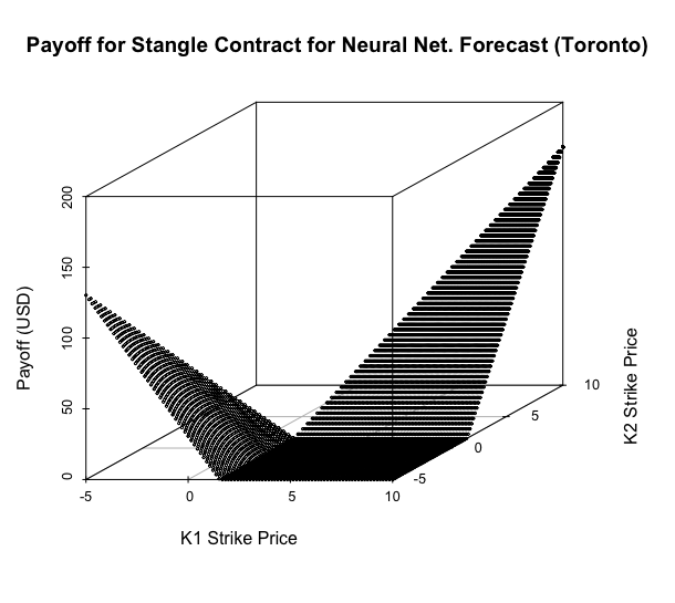
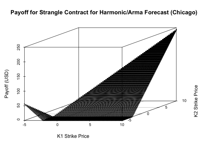
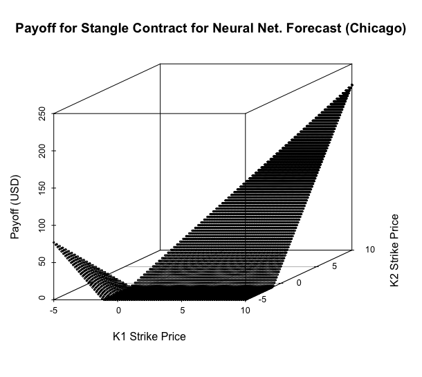
Because a strangle contract can provide a payoff when temperatures are much higher or lower this contract could be especially useful in addressing economic issues related to climate change as temperatures become more volatile and less predictable. Figures 12(a) and 12(b) show a three dimensional scatter plot of the payoffs for the same contract when for different strike prices. Here the strike price for a call is unrelated to the strike price for the put with the exception that .
| Method | PR Toronto | PR Chicago | |
|---|---|---|---|
| Actual value of PR | 3.304 | 1.83 | |
| 40 Year Average | -0.1634146 | -3.217561 | |
| Harmonic Regression | 0.8564685 | -2.477111 | |
| Harmonic/ARMA model | 0.7683072 | -2.17967 | |
| Neural Network model | 1.541371 | -1.137333 |
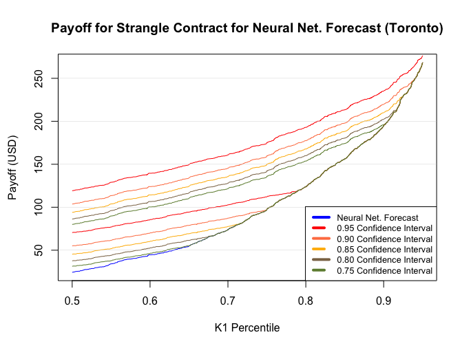
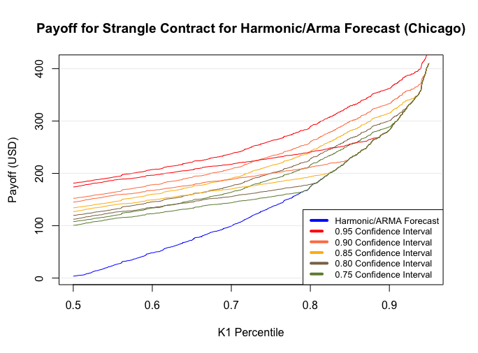
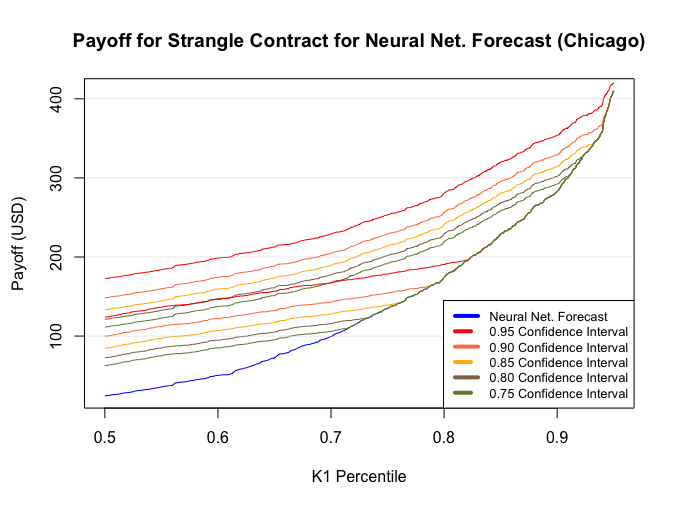
A scatter plot of the the Pacific Rim for Chicago from 1981-2023 also shows the index is increasing. Figures 13(a) and 13(b) show the estimated payoff for a strangle based on the forecast of the Harmonic/ARMA and neural network model. In these figures the value is the strike price for the call option given in terms of percentiles of the mean temperature for the month of December. We can see that when the strike prices are chosen as percentiles of historical temperatures as explained in the introduction to this section we get a non-linear increase in the payoff of the contract. In figures 14(a) and 14(b) where we can see the payoff for our harmonic/ARMA model and neural network model when we pick unrelated strike prices we see that the payoff for our contract increases linearly.
5.2. Pricing Toronto and Chicago precipitation contracts
We show prices of WD contracts based on precipitation for the month of December. The cumulated precipitation follows equation (1) with a Gamma distribution for the daily amounts. The parameters of the Gamma distribution have been estimated in section 4 using a CNN and a MLE approach. It allows to make a forecast for daily cumulative precipitation for December 2023 by computing the integrals and in equation (5).
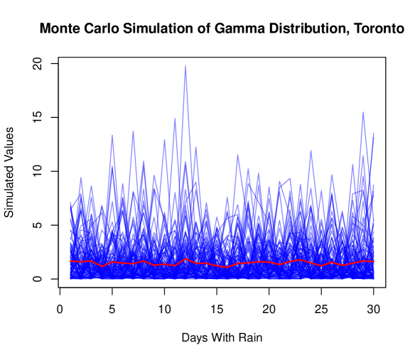
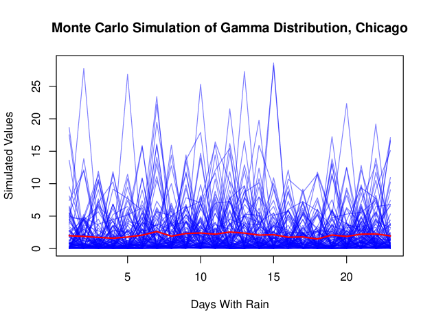
By mean of the estimated values and also we can perform a Monte Carlo simulation for precipitations in Toronto and Chicago. The no raining days are modeled through a Poisson Process with parameter . We estimated the later by taking the average number of days it rains in December each year, from 1981-2023. In total, an estimate of the DTP for December is obtained after 1000 simulations.
Graphs showing the simulated values of precipitation for Toronto and Chicago can be seen in figures 15(a) and 15(b) respectively. Each blue line in this graph represents one simulation for December, and the red line represents the mean of all the simulated values. If we take the mean value of this red line this would provide us with an estimate for the Pacific Rim index.
The price of the WD contract can be obtained by directly computing integrals and . Notice that the sum of independent Gamma distributed random variables, independent and equally distributed is also Gamma distributed with parameters and . Hence the p.d.f. of the Pacific Rim index is:
| (8) |
On the other hand, after elementary transformations we have:
| (9) | |||||
| (10) |
Similarly:
| (11) |
By using the prices for a call and put option we can compute a pricing formula for a strangle contract, as in equation 5.2.
Thus, using the upper-incomplete, lower-incomplete, and complete gamma function we can easily calculate the estimated payoff of a call, put, or strangle contract where precipitation is modeled using a compound Poisson process with the gamma distribution.
Gathering both terms and and replacing in the price formula (5) we have the final price given by:
| (12) |
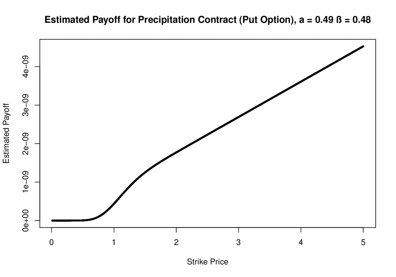
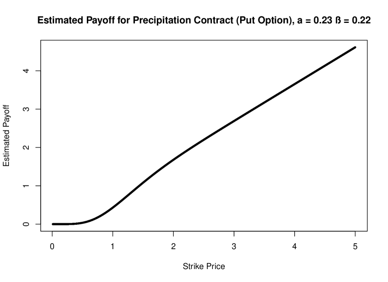
In figures 16(a) and 16(b) we can see the price of the part of the contract defined by the call option as function of the strike price for both cities. In both figures the and values are the hyper-parameter values produced from the convolutional neural network in Section 4.2. We chose to use the estimates from the CNN because this method does not assume i.i.d. conditions, which is not an assumption supported by empirical evidence.
6. Conclusions and recommendations
In this paper we have considered a neural network technique to price weather derivative contracts based on a Pacific Rim index for temperatures and precipitations. The results have been compared to a method based on a traditional time-series models.
Results for the case of Toronto and Chicago cities show that neural networks are better able at forecasting daily average temperature for the purpose of pricing weather derivative contracts. Based on the MSE of the forecasts we come to the conclusion that a neural network approach can better capture the complex dynamics of temperature forecasting.
In connection with precipitation contracts, to estimate the hyper parameters of a gamma distribution in the amount of daily precipitation we trained a convolutional neural network on generated data along with a MLE estimation procedure. A CNN approach assumes that the precipitation data is represented within the simulated training set of our CNN. Although the MLE has a lower standard error than those obtained from CNN, the later do not require the unrealistic assumption of independence between daily precipitation.
References
- [1] A. K. Alexandridis and A. D. Zapranis. Weather Derivatives: Modeling and Pricing Weather-Related Risk. Springer, 2013.
- [2] Jason Brownlee. Deep Learning for Time Series Forecasting-Predict the Future with MLPs, CNNs and LSTMs in Python. 2018.
- [3] Roberto Buizza and James W. Taylor. A comparison of temperature density forecasts from garch and atmospheric models. Journal of Forecasting, 23(5):337–355, 2004.
- [4] Sean D Campbell and Francis X Diebold. Weather forecasting for weather derivatives. Journal of the American Statistical Association, 100(469):6–16, 2005.
- [5] Jonathan D.Cryer and Kung-Sik Chan. Time Series Analysis With Applications in R. Springer, 2018.
- [6] Sergey Ioffe and Christian Szegedy. Accelerating deep network training by reducing internal covariate shift. arXiv, 2015.
- [7] Gareth James, Daniela Witten, Trevor Hastie, and Robert Tibshirani. An Introduction to Statistical Learning with Applications in R. Springer, 2013.
- [8] Stephen Jewson and Anders Brix. Weather derivative valuation: the meteorological, statistical, financial and mathematical foundations. Cambridge University Press, 2005, 2005.
- [9] P. Olivares and E. Villamor. Pricing temperature derivatives under a time-changed levy model. https://arxiv.org/abs/2005.14350, 2020.
- [10] Brockwell P.J. and Davis R.A. Time Series: Theory and Methods, 3rd editon. Springer. New York, 2016.
- [11] Achilleas Zapranis and Antonis Alexandridis. Weather derivatives pricing: Modeling the seasonal residual variance of an ornstein-uhlenbeck temperature process with neural networks. Technical report, University of Macedonia, December 2009.