SynCoTrain: A Dual Classifier PU-learning Framework for Synthesizability Prediction
Abstract
Material discovery is a cornerstone of modern science, driving advancements in diverse disciplines from biomedical technology to climate solutions. Predicting synthesizability, a critical factor in realizing novel materials, remains a complex challenge due to the limitations of traditional heuristics and thermodynamic proxies. While stability metrics such as formation energy offer partial insights, they fail to account for kinetic factors and technological constraints that influence synthesis outcomes. These challenges are further compounded by the scarcity of negative data, as failed synthesis attempts are often unpublished or context-specific.
We present SynCoTrain, a semi-supervised machine learning model designed to predict the synthesizability of materials. SynCoTrain employs a co-training framework leveraging two complementary graph convolutional neural networks: SchNet and ALIGNN. By iteratively exchanging predictions between classifiers, SynCoTrain mitigates model bias and enhances generalizability. Our approach uses Positive and Unlabeled (PU) Learning to address the absence of explicit negative data, iteratively refining predictions through collaborative learning.
The model demonstrates robust performance, achieving high recall on internal and leave-out test sets. By focusing on oxide crystals, a well-characterized material family with extensive experimental data, we establish SynCoTrain as a reliable tool for predicting synthesizability while balancing dataset variability and computational efficiency. This work highlights the potential of co-training to advance high-throughput materials discovery and generative research, offering a scalable solution to the challenge of synthesizability prediction.
1 Introduction
Material discovery is a foundational pillar of modern science and perhaps the driving motivation behind materials science. It supports advancements in numerous scientific and technological disciplines. In this field, the ability to predict synthesizability is crucial. Developing materials with novel properties expands the possibilities in endeavors from functional materials used in biomedical devices to addressing the challenges of climate change [1]. In the past decade or so, efforts such as the Materials Genome Initiative aimed to accelerate the discovery, development, and deployment of new materials in the hopes of societal betterment [1, 2]. An essential part of realizing this goal is employing high-throughput simulations and experiments for screening candidate materials with desirable properties [1, 3]. Unfortunately, a substantial amount of resources and effort can be wasted on hypothetical materials that currently cannot be synthesized.
Historically, physico-chemical based heuristics such as the Pauling Rules [4] or the charge-balancing criteria [5] have been used to assess materials stability and synthesizability. Nevertheless, these simplified approaches have been shown to be out of date, as more than half of the experimental (already synthesized) materials on the Materials Project database [6] do not meet these criteria for synthesizability [5, 7].
In more recent attempts, material scientists often employed thermodynamic stability as a proxy for synthesizability, ignoring the effect of kinetic stabilization. This involves conducting first-principle calculations to estimate the formation energy of crystals and their distance from the convex hull. A negative formation energy, or a minimal distance from the convex hull, is commonly interpreted as an indicator of synthesizability [8, 9, 10, 11, 12]. While stability significantly contributes to synthesizability, it is just one aspect of this complex issue. There are many -potentially interesting- metastable materials that do exist, even though their formation energies deviate from the ground-state [8, 11, 13, 14, 15]. These materials can be synthesized in alternate thermodynamic conditions in which they are the ground-state. After removing the favorable thermodynamic field, they have stayed stuck in the metastable structure by kinetic stabilization [8]. On the other hand, there are many hypothetical stable materials in well-explored chemical spaces which have never been synthesized. This could be due to a high activation energy barrier between them and the common precursors [13, 14, 15]. Beyond the theoretical and thermodynamic considerations, synthesizability is also a technological problem. Novel materials that are developed through cutting-edge methods were practically unsynthesizable before the invention of their methods of synthesis. For example, new high-entropy alloys with great potential for catalysis applications were recently synthesized using the Carbothermal Shock (CTS) method [16]. Their particular homogeneous components and uniform structures were not accessible through conventional synthesis methods. On the other hand, some materials can only be synthesized under specific conditions, such as extremely high pressures [17] or within solvents like liquid ammonia [18], which alter their chemical behavior. Once these conditions are removed, however, the materials may decompose.
The fact that estimating synthesizability is related to materials structures without a straightforward formula to solve for, makes it an apt candidate for machine learning. We define a classification task for two classes of materials, namely synthesizable (the positive class), and unsynthesizable (the negative class). This classification comes with a few challenges and intricacies. The first one is encoding materials structures in a machine understandable format. Some previous works have circumvented this challenge in creative ways such as combining different elemental features [15, 19], using text-mining algorithms to search the relevant literature to identify synthesizable materials [20], using the picture of crystal cells with convolutional neural networks [21], or even a network analysis of materials discovery timeline with respect to their stability [22]. Others [14, 23], including this work, utilize graph convolutional neural networks (GCNNs) to encode and learn from crystal structures. While the GCNNs are more complicated to implement, they have the advantage of including more information about the structure than composition alone or the other previously mentioned approaches that represent the structure information indirectly through a proxy.
The second challenge of estimating synthesizability lies within the nature of the available data. Unlike a typical classification task, we do not have access to enough negative data. On the one hand, this is due to the fact that unsuccessful attempts of synthesis are not typically published nor uploaded to public databases. The attempts of using such failed experiments [24] inevitably remain confined to local labs and a small class of materials. Also, synthesis success strongly depends on the synthesis conditions and technology. Hence, the failure of synthesis attempts in one setting does not necessarily imply failure in a different lab with different synthesis methods or equipment. Finally, creating a proper negative-set for training a classifier is a whole new challenge [5]. If the negative-set is too different from real materials, it may not teach the model a meaningful decision boundary for detecting synthesizability. To design a realistic-looking negative-set, one would need to understand the features that determine synthesizability in the first place.
The final challenge in this task comes as a fundamental aspect of machine learning. Regardless of which model is chosen, it will inherently exhibit a certain degree of bias. One introduces an unintended bias when selecting one model over another, since the model’s ability to generalize out of sample is, in part, predetermined by its architecture. This model bias comes even with the best performing models. In fact, a model with great benchmarks might perform worse than simpler models when predicting targets for out-of-distribution data [25], perhaps due to overfitting. This challenge becomes particularly pronounced when predicting synthesizability. The objective is to forecast a target for new and often out-of-distribution data, where the issue of generalization is most acute. The lack of the negative data compounds this issue, as it makes the accuracy or recall less reliable. One way to mitigate this inherent bias is to leverage multiple models [25].
To address these challenges, we have developed a model ready for integration into high-throughput simulations and generative materials research. It is called SynCoTrain (pronounced similar to ’Synchrotron’). It is a semi-supervised classification model designed for predicting synthesizability of oxide crystals. SynCoTrain addresses the generalizability issue by utilizing co-training. Co-training is an iterative semi-supervised learning process designed for scenarios with some positive data and a lot of unlabeled data [26, 27]. It leverages the predictive power of two distinct classifiers to find and label positive data points among the unlabeled data. Different models have different biases, and by combining their predictions, we can practically reduce these biases while keeping what they learn about the target. We use the Atomistic Line Graph Neural Network (ALIGNN) [28] and the SchNetPack [29, 30] models as our chosen classifiers. They are both innovative GCNNs with distinct attributes. ALIGNN is unique in that it directly encodes both atomic bonds and bond angles into its architecture, offering a perspective that aligns with a chemist’s view of the data. SchNetPack stands out for using a unique continuous convolution filter which is suitable for encoding atomic structures, which can be thought of as a physicist’s perspective on the data.
At each step of co-training, SynCoTrain learns the distribution of the synthesizable crystals through the Positive and Unlabeled Learning (PU Learning) method introduced by Mordelet and Vert [31]. This base PU Learning method with a different classifier has already been employed to predict synthesizability for all classes of crystals [14] and for perovskites specifically [23]. In this work, we utilize multiple PU Learners as the building blocks for co-training. In each iteration of co-training, the learning agents exchange the knowledge they gained from the data between each other. Eventually, the labels are decided based on average of their predictions. This process increases the prediction reliability and accuracy, much like two experts who discuss and reconcile their views before finalizing a complex decision. This collaborative approach suggests that co-training is more likely to generalize effectively to unseen data compared to using a single model with equivalent classification metrics such as accuracy or recall.
We verify the performance of the model by recall for an internal test-set and a leave-out test-set. We also evaluate our model further by predicting whether a crystal is stable or not for the same data points. Note that in predicting stability, we do not aim for a good performance. In fact, we expect an overall poor performance due to high contamination of the unlabeled data [31]; more info in supplemental material. However, we compare the ground truth recall in stability to the recall produced by the PU Learning, to gauge the reliability of the latter.
We chose a single family of materials, oxides, to establish the utility of co-training in predicting materials properties. Oxides are a well-studied class of materials with a large amount of experimental data to learn from [32, 33]. A higher number of training data would typically decrease the classification error in machine learning. However, training across all available families of crystals would introduce greater variability in the dataset, potentially increasing the uncertainty and error margins in our results. In other words, the prediction quality for new materials would vary substantially. By achieving high recall values with oxides as our training data, we demonstrate the effectiveness of co-training. This approach ensures reliable results while maintaining reasonable training times for our models.
2 Results and Discussion
2.1 Model Development
The data for oxide crystals were obtained from the Inorganic Crystal Structure Database (ICSD) [34], accessed through the Materials Project API [6]. The experimental and theoretical data are distinguished based on the ‘theoretical’ attribute. We used the get_valences function of pymatgen [35] to include only oxides where the oxidation number is determinable and the oxidation state of oxygen is -2.
Less than 1% of the experimental data with energy above hull higher than 1eV were removed, as potentially corrupt data. The learning began with 10206 experimental and 31245 unlabeled data points.
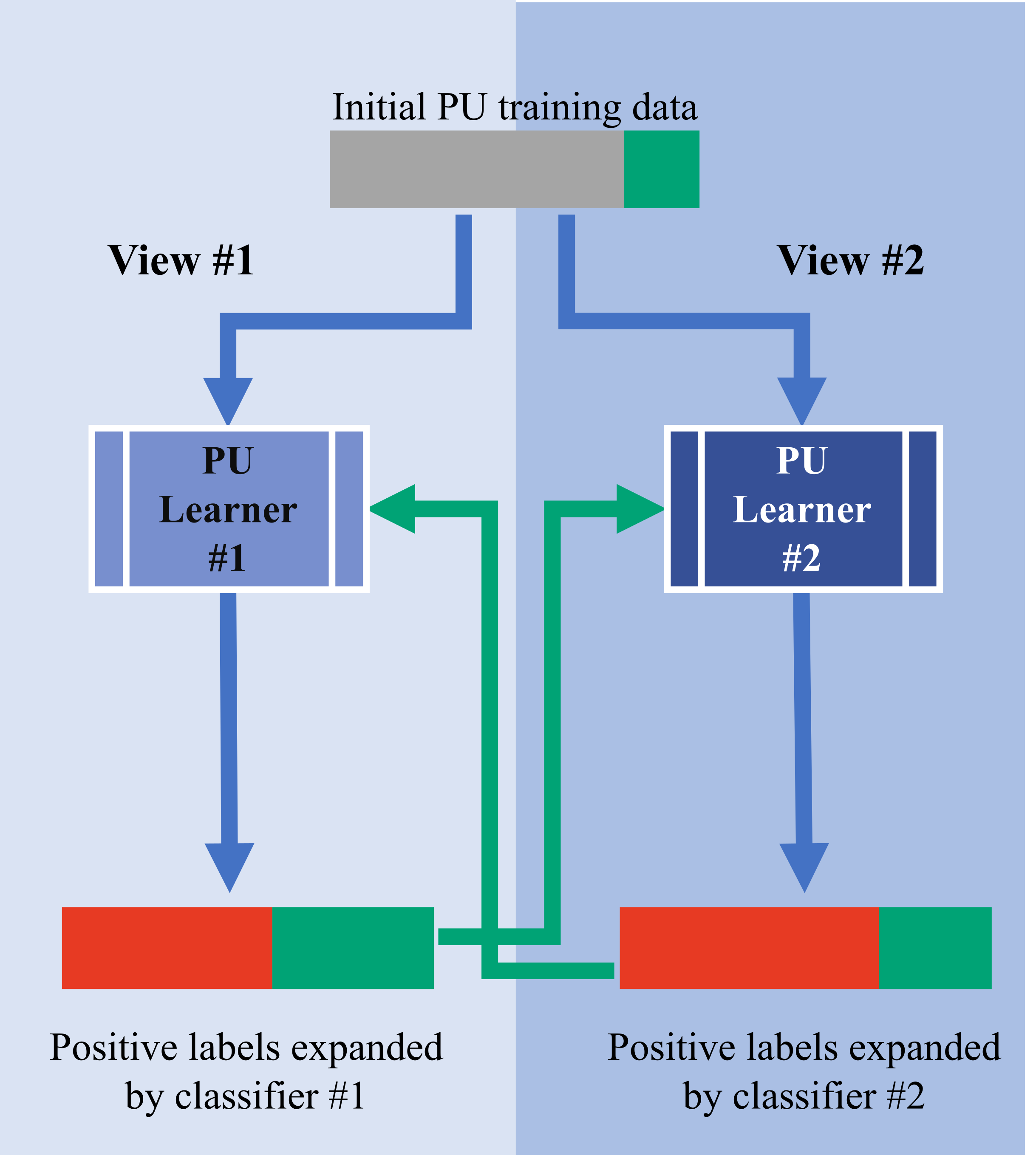
Co-training consists of two separate iteration series, the results of which are averaged in the final step. In the first series, we start by training a base PU learner with an ALIGNN classifier. This is the iteration ‘0’ of co-training, and this step is called ALIGNN0. The learning agent predicts positive labels for some of the unlabeled data, creating a pseudo-positive class. This class is added to the original experimental data, expanding the initial positive class. Iteration ‘1’ of co-training on this series is to train a base PU learner with the other classifier, here the SchNet, on the newly expanded labels. This step is called coSchnet1. Each iteration provides newly expanded labels for the next iteration. The classifiers alternate for each iteration, from ALIGNN to SchNet and vice versa, as shown in Fig. 1(a).
Parallel to this series, we set up a mirror series where iteration ‘0’ begins with a SchNet based PU learner. This step of iteration ‘0’ is called SchNet0. This series learns the data from a different, complementary view compared to the former series, see Fig. 1(a). It continues in the same manner with alternating classifiers. The order of the steps in each series can be found in Table 1.
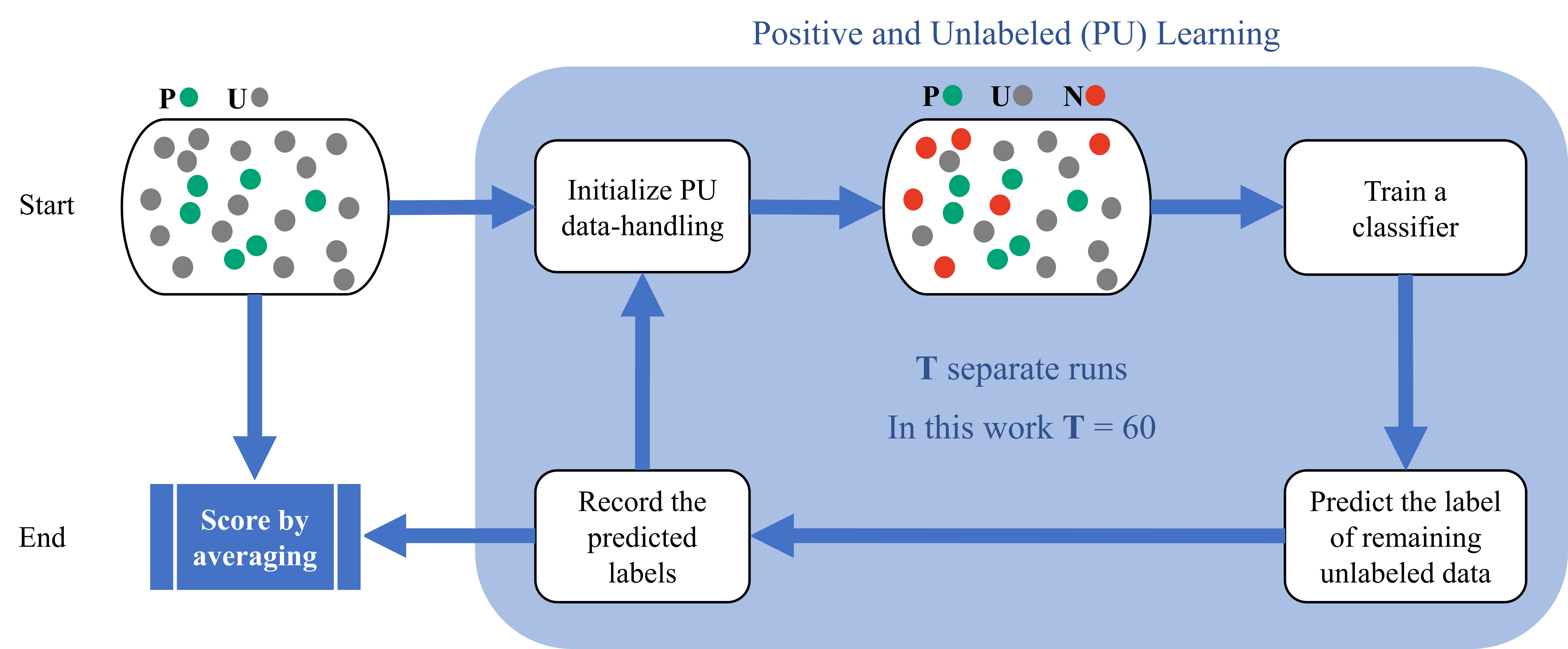
Each base PU learner produces a synthesizability score between 0 and 1 for each unlabeled datum. This is done through 60 runs of the bagging method established by Mordelet and Vert [31], as illustrated in Fig. 1(c). In each independent run of this ensemble learner, a random subset of the unlabeled data is sampled to play the role of the negative data in training the classifier. The average of the predictions in these runs for data points that were not part of the training in that run yields the synthesizability score. This score is interpreted as the predicted probability of being synthesizable. A threshold of 0.5 is applied for labeling each datum as either synthesizable (labeled 1) or not-synthesizable (labeled 0).
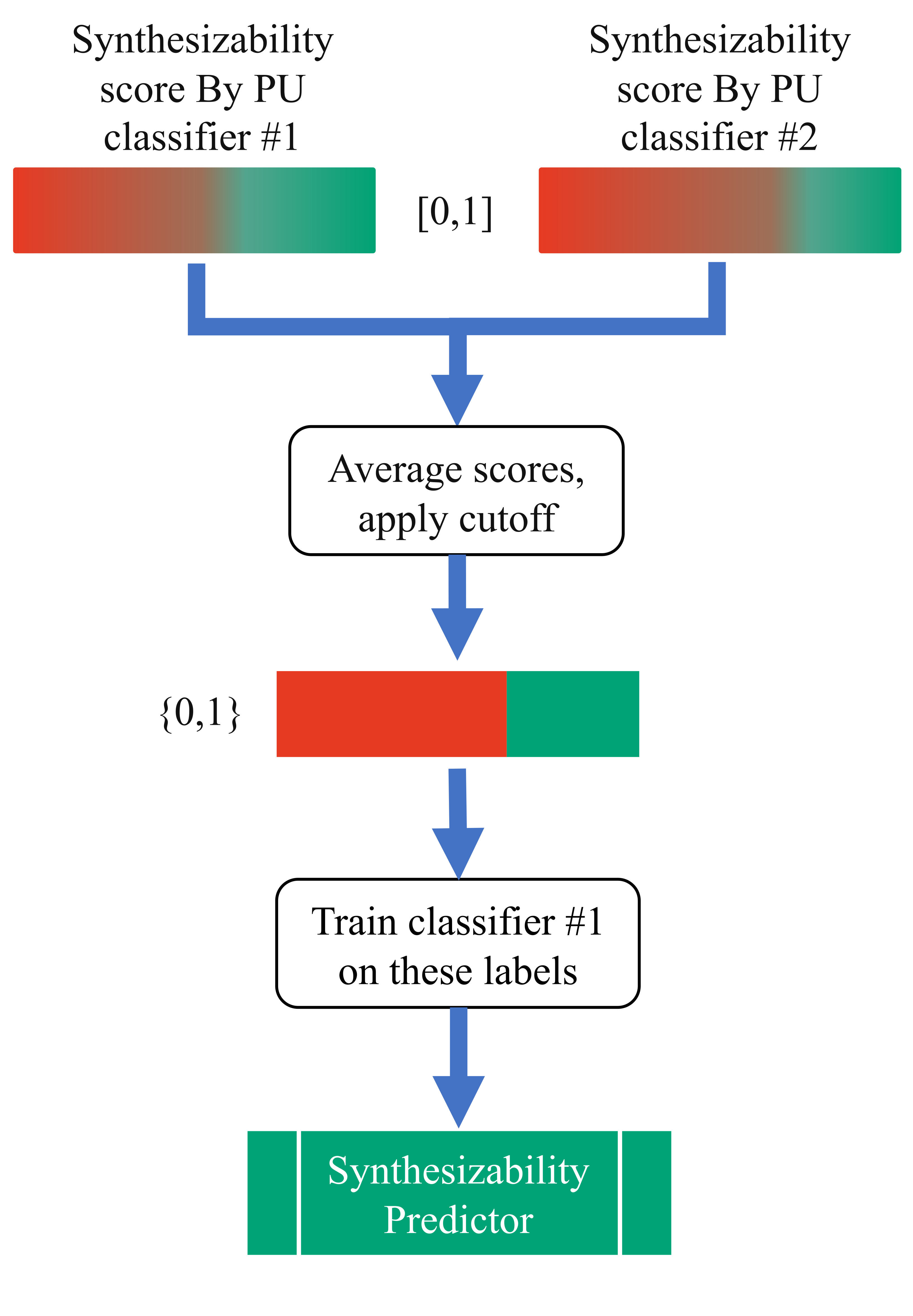
After several iterations of co-training, the optimal iteration is chosen based on the prediction metrics. Continuing to further iterations yields diminishing returns in performance metric while risking reinforcing existing model bias. The scores provided from the two series at the optimal iteration are then averaged. The 0.5 cutoff threshold is applied to this averaged score to produce the final synthesizability score. Once we have synthesizability labels for both the experimental and theoretical data, a simple machine learning task remains. We train a classifier on these labels and end up with a model that can predict synthesizability (see Fig. 1(b)).
| Co-training steps | Iteration ‘0’ | Iteration ‘1’ | Iteration ‘2’ | Iteration ‘3’ | Averaging scores | |||
|---|---|---|---|---|---|---|---|---|
| Training data source |
Original
labels |
Labels
expanded by Iteration ‘0’ |
Labels
expanded by Iteration ‘1’ |
Labels
expanded by Iteration ‘2’ |
Scores provided
by the optimal iteration |
|||
| Training series | ALIGNN0 | > | coSchnet1 | > | coAlignn2 | > | coSchnet3 | Synthesizability scores |
| SchNet0 | > | coAlignn1 | > | coSchnet2 | > | coAlignn3 |
2.2 Model Evaluation and Results
Within each single run of the base PU Learning, the classifiers optimize for Accuracy, as they operate unaware of the PU nature of the data. When reporting the performance of PU learning, however, one should not use Accuracy, Precision or the F1-score. These common measures assume knowledge of the negative labels and a False Positive count. We use Recall, also known as Sensitivity or True Positive Rate (true positive/(true positive + false negative)) to report and benchmark the performance of our PU learner as it only relies on the knowledge of the positive data.
In our study, we employ two distinct test-sets to measure Recall. The first is a dynamic test-set, which varies with each iteration of base PU learning. The second is a leave-out test-set that remains untouched during all training iterations. As the result, we obtain a ‘recall range’ between the two distinct Recall measures; an averaged recall for the dynamic test-set and a leave-out recall. This gives us more information than a single recall value. The construction and reasoning behind this are detailed in the Ground Truth evaluation section.
The construction and reasoning behind this are detailed in the Ground Truth evaluation section.
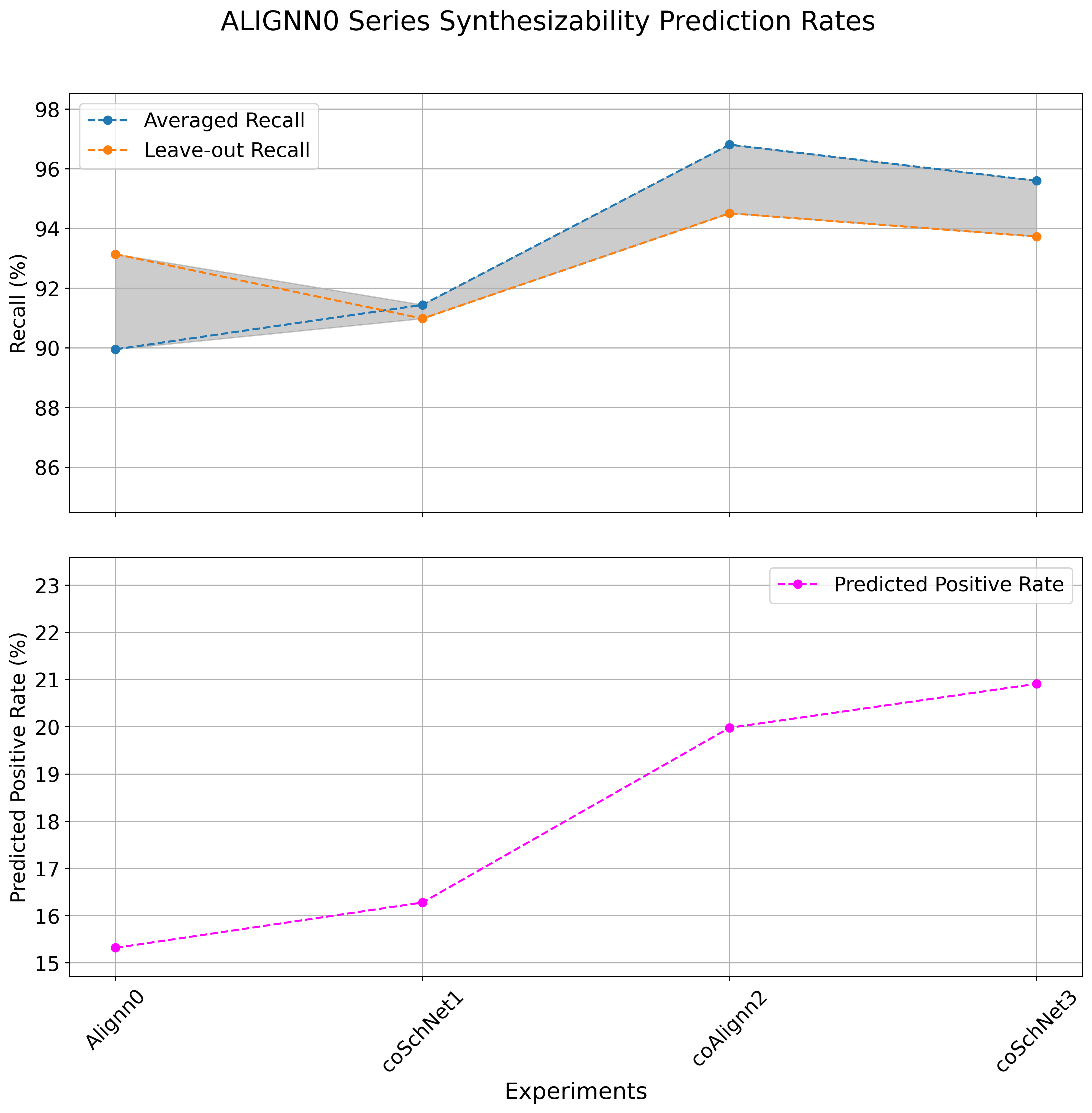
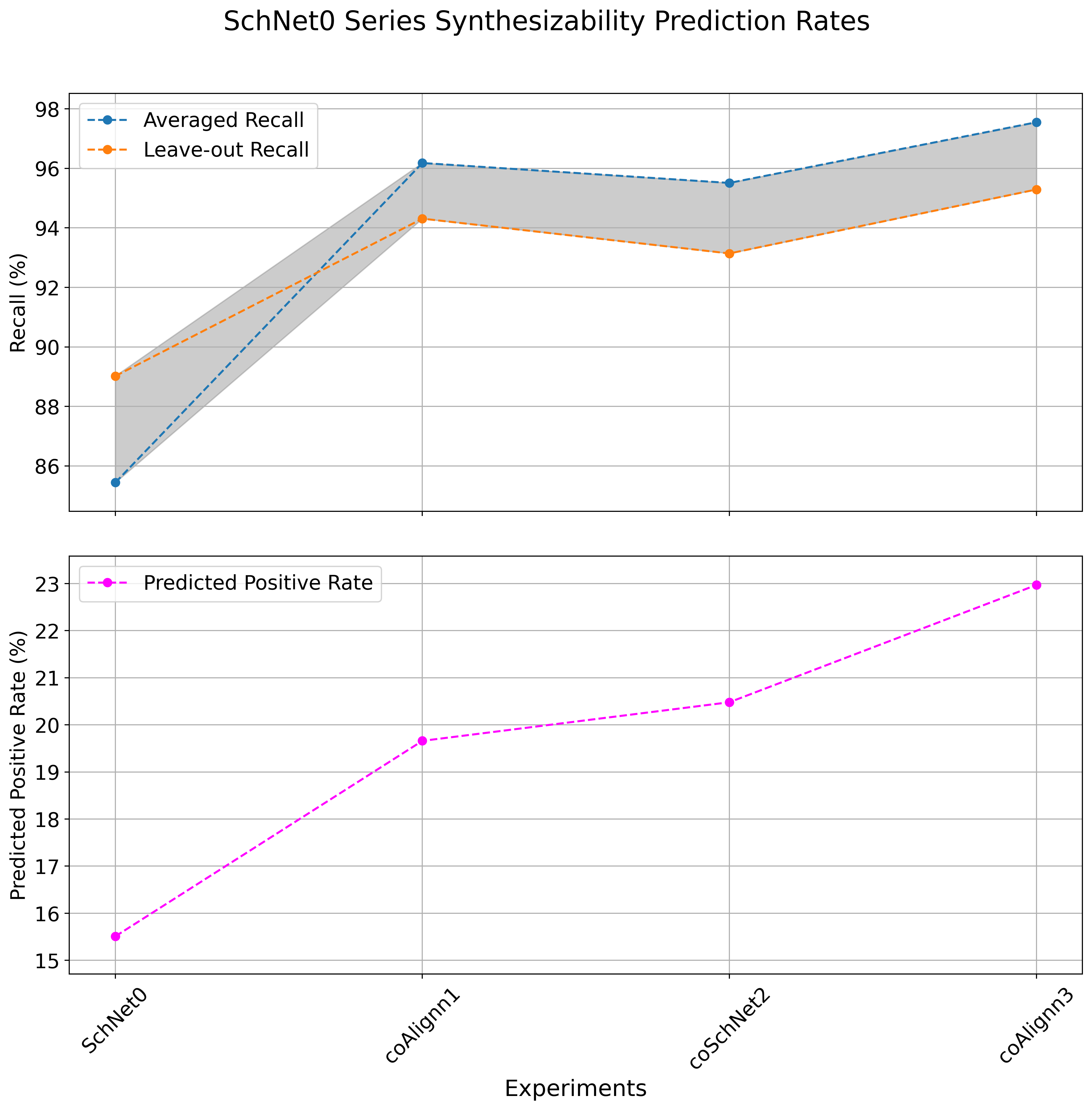
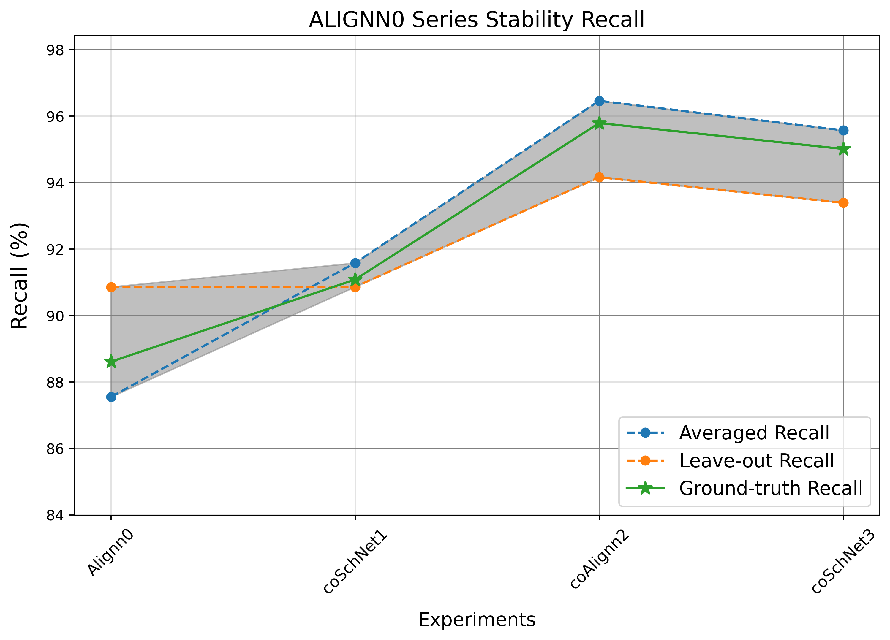
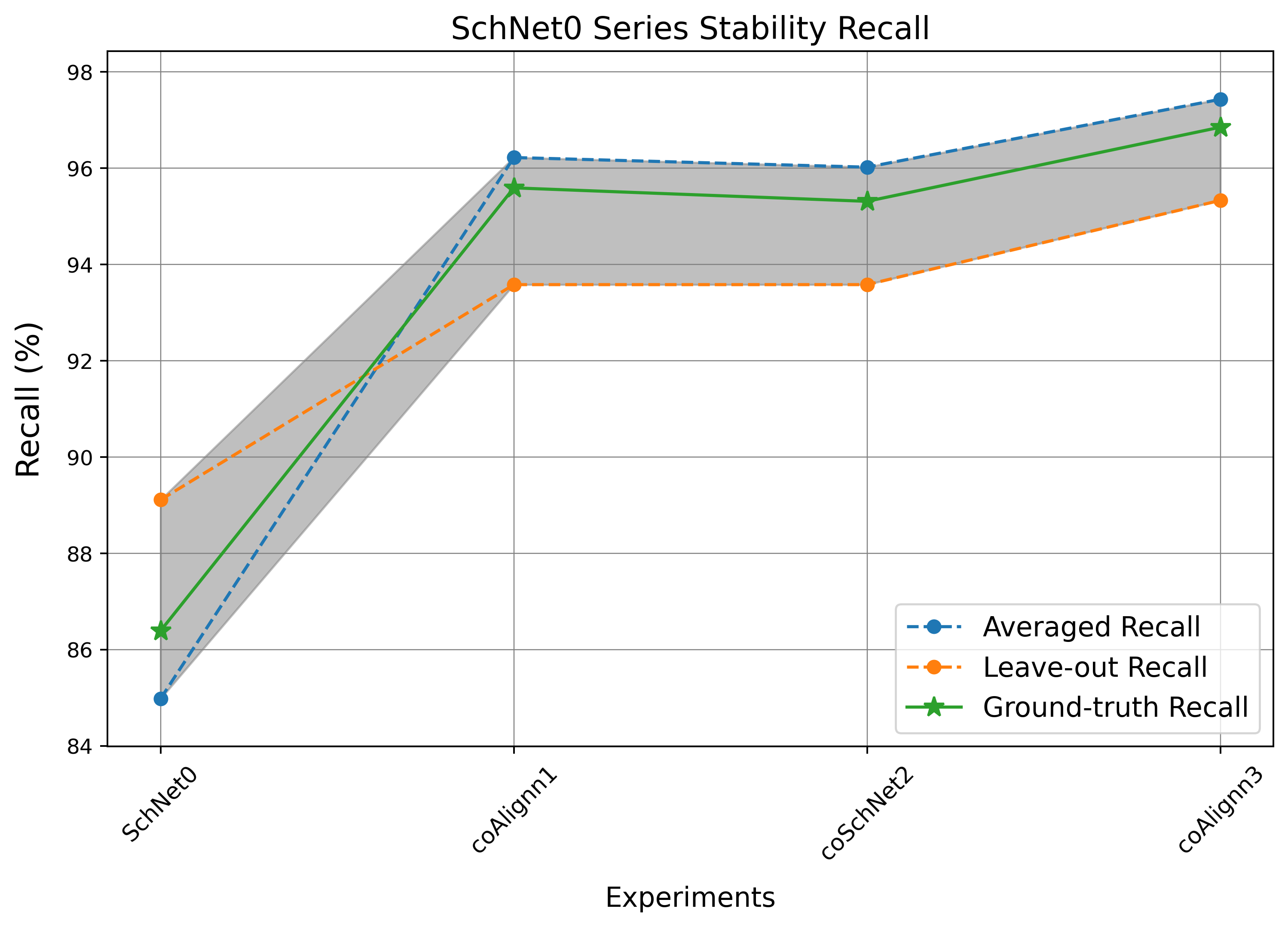
The recall values for each iteration are depicted in Fig. 2. The two distinct co-training series are separately visualized to clearly illustrate Recall changes at each step. We see that the SchNet0 series somewhat plateaus in iteration ‘2’, while the ALIGNN0 series still improves in recall. However, neither series make significant improvement on their recall in iteration ‘3’. This suggests that using the third iteration yields diminishing returns in terms of new learning, while risking enforcing models’ biases through too many repetitions. Furthermore, the predicted positive rate increases in both series for iteration ‘3’, without a meaningful increase in recall range to justify it. This means that the model is more likely to classify a theoretical crystal as synthesizable, without improving its understanding of synthesizability. This is akin to over-fitting, when additional learning steps do not yield better validation results. These factors indicate that iteration ‘2’ is optimal. Consequently, we omit the third iteration and use the results from iteration ‘2’ as the source for synthesizability labels.
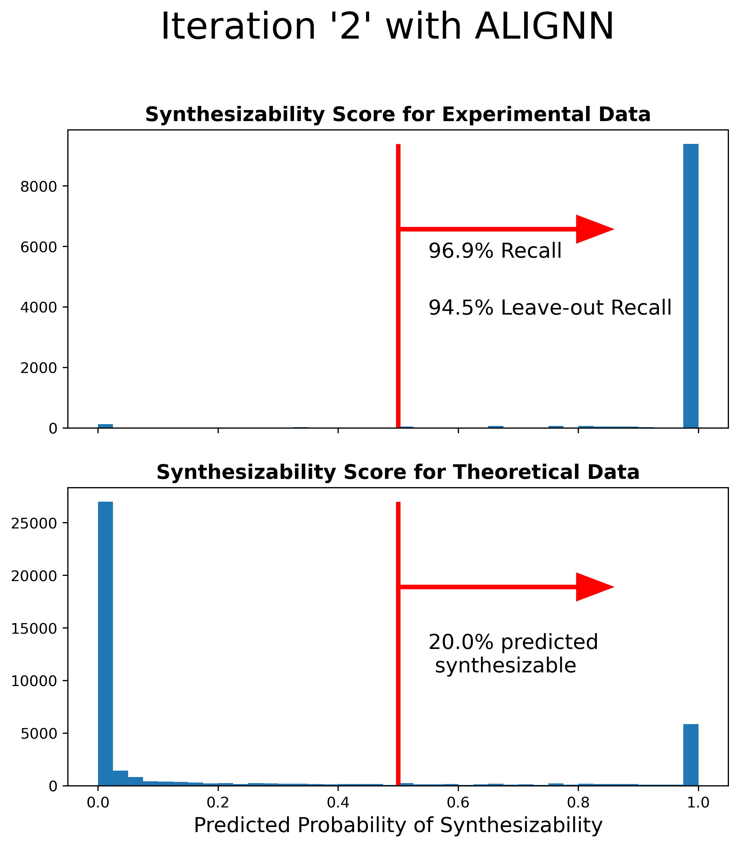
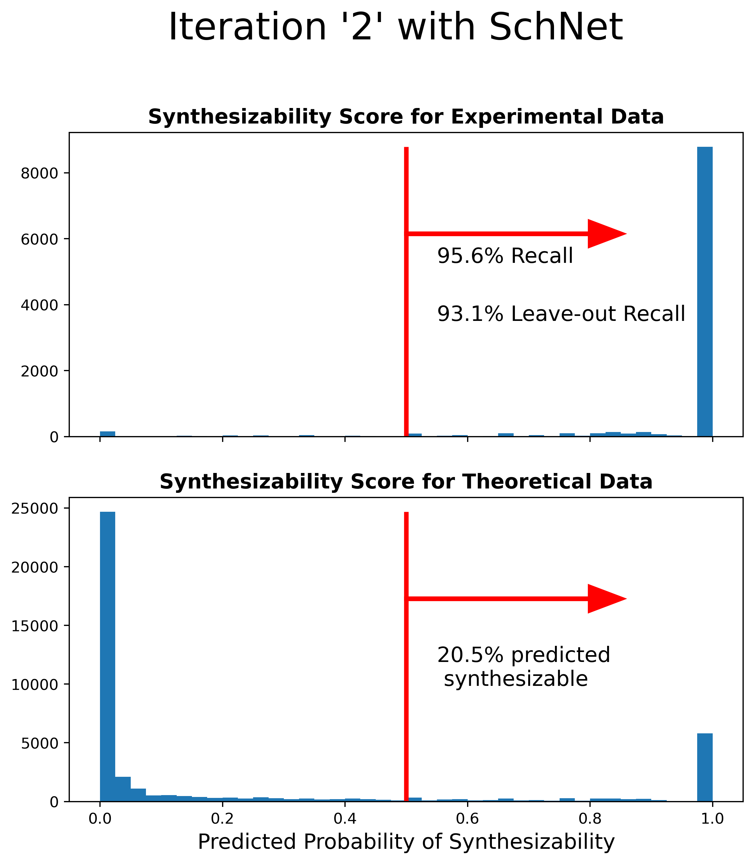
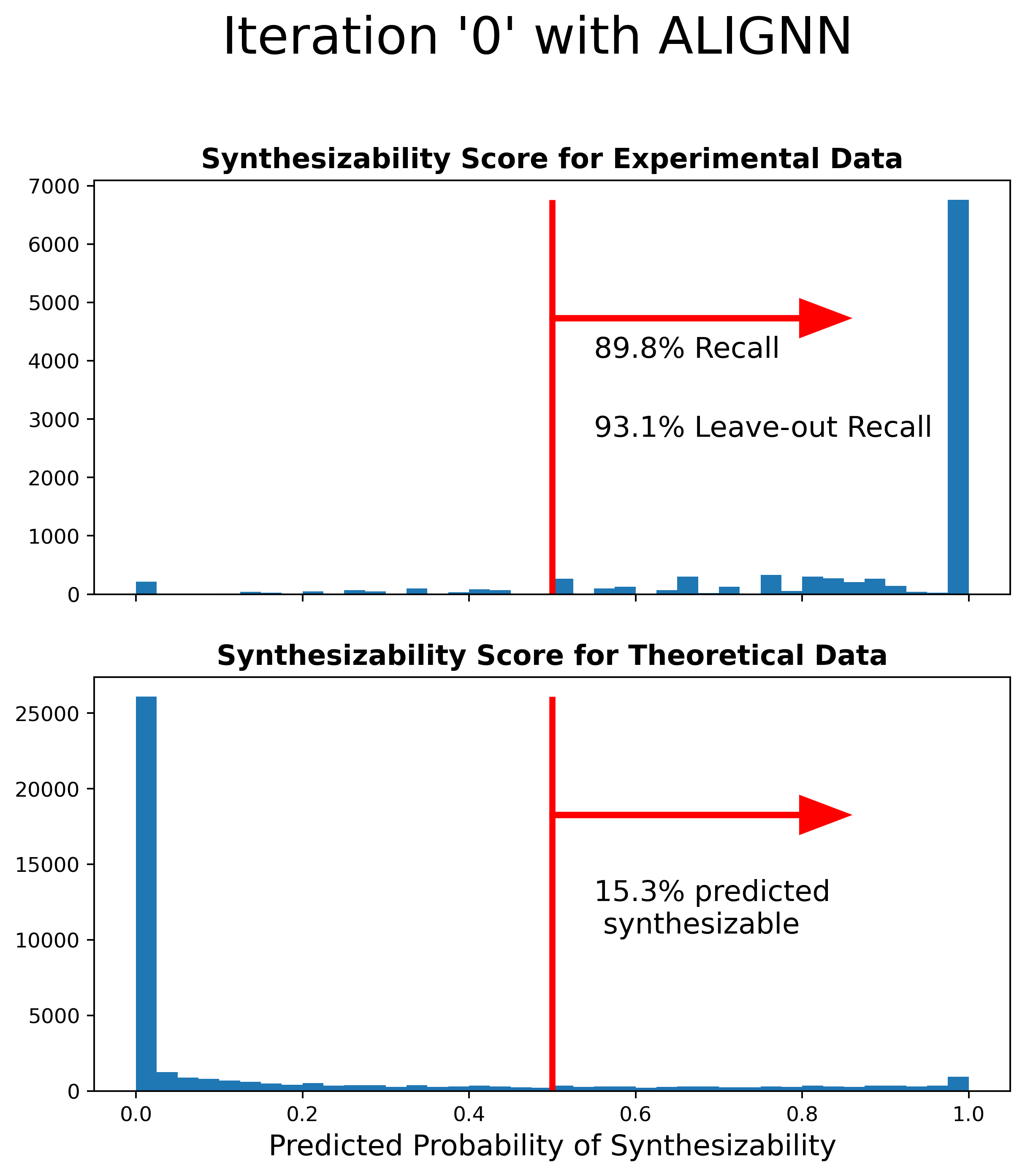
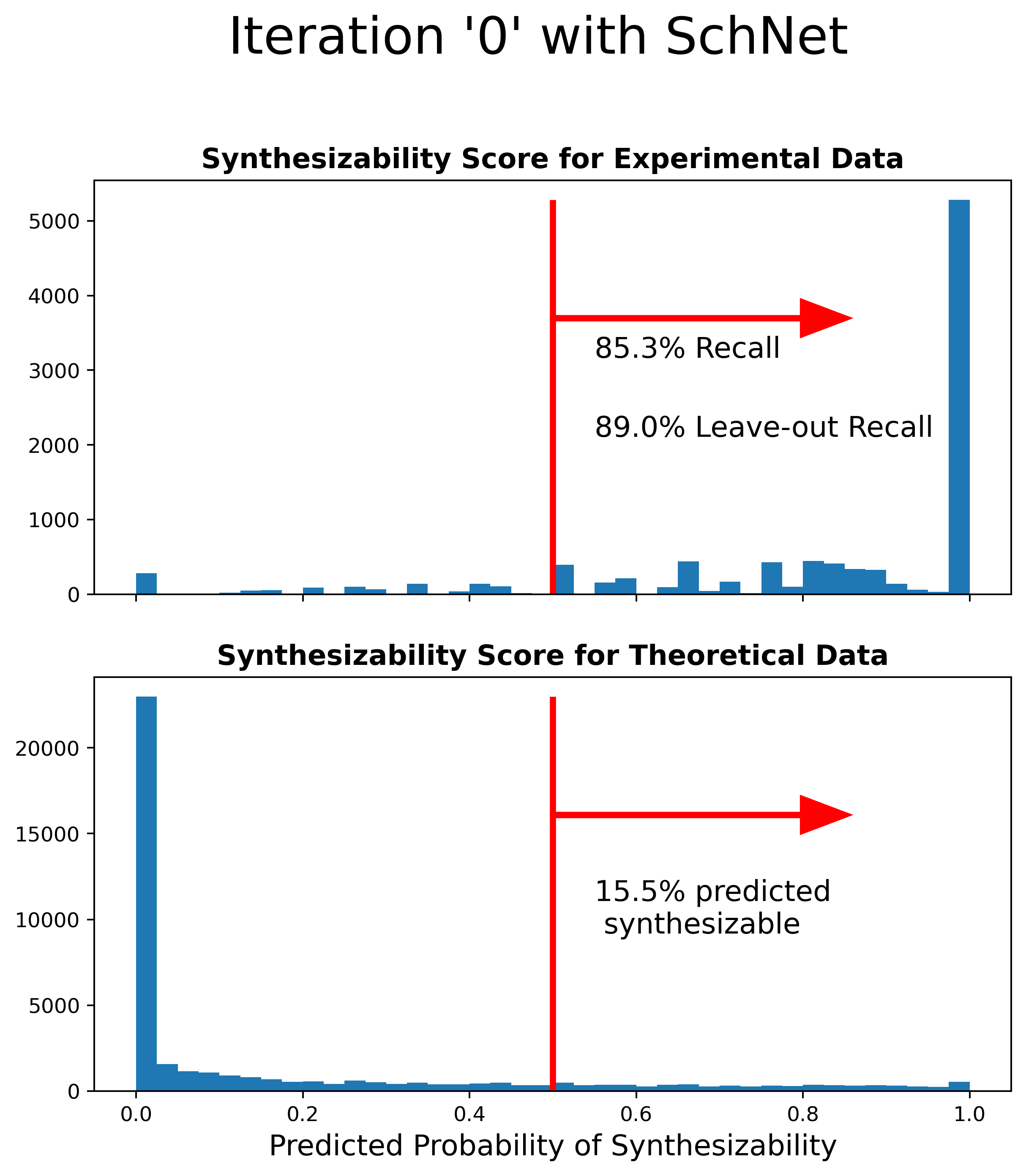
The synthesizability scores provided for the unlabeled data is the actual goal of this PU learning task. The distribution of these scores, alongside a large Recall rate, provide a sense of the performance quality. A model that marks almost all crystals as synthesizable would have a high recall but could not distinguish the two classes from each other. Fig. 3 and Fig. 4 show the distributions of synthesizability scores at iteration ‘0’ and iteration ‘2’ of co-training, respectively. Despite high recall values, the PU learners mark only about 20% of the unlabeled data as synthesizable. The synthesizability scores for the intermediate iterations can be found in the supplementary materials.
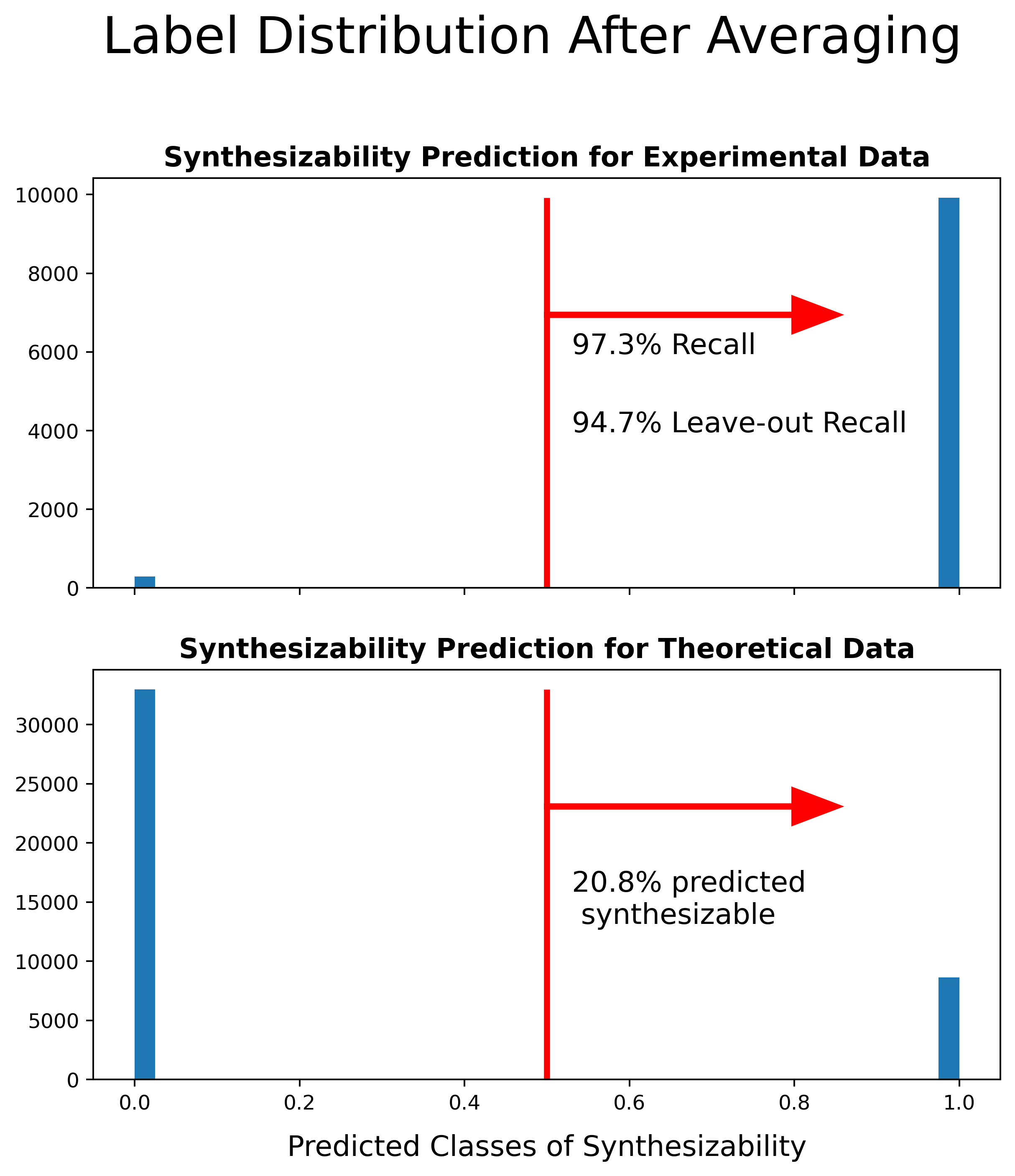
In the final step of co-training, the scores from iteration ‘2’ are averaged and final labels are predicted via a cutoff of 0.5. This yields the final labels to for training the synthesizability predictor. The recall range is now [95-97]% and 21% of the unlabeled data are predicted to be synthesizable, see Fig. 5. Of course, all experimental data, including the ~3% that were misclassified as unsynthesizable, are labeled as positive for training the synthesizability predictor.
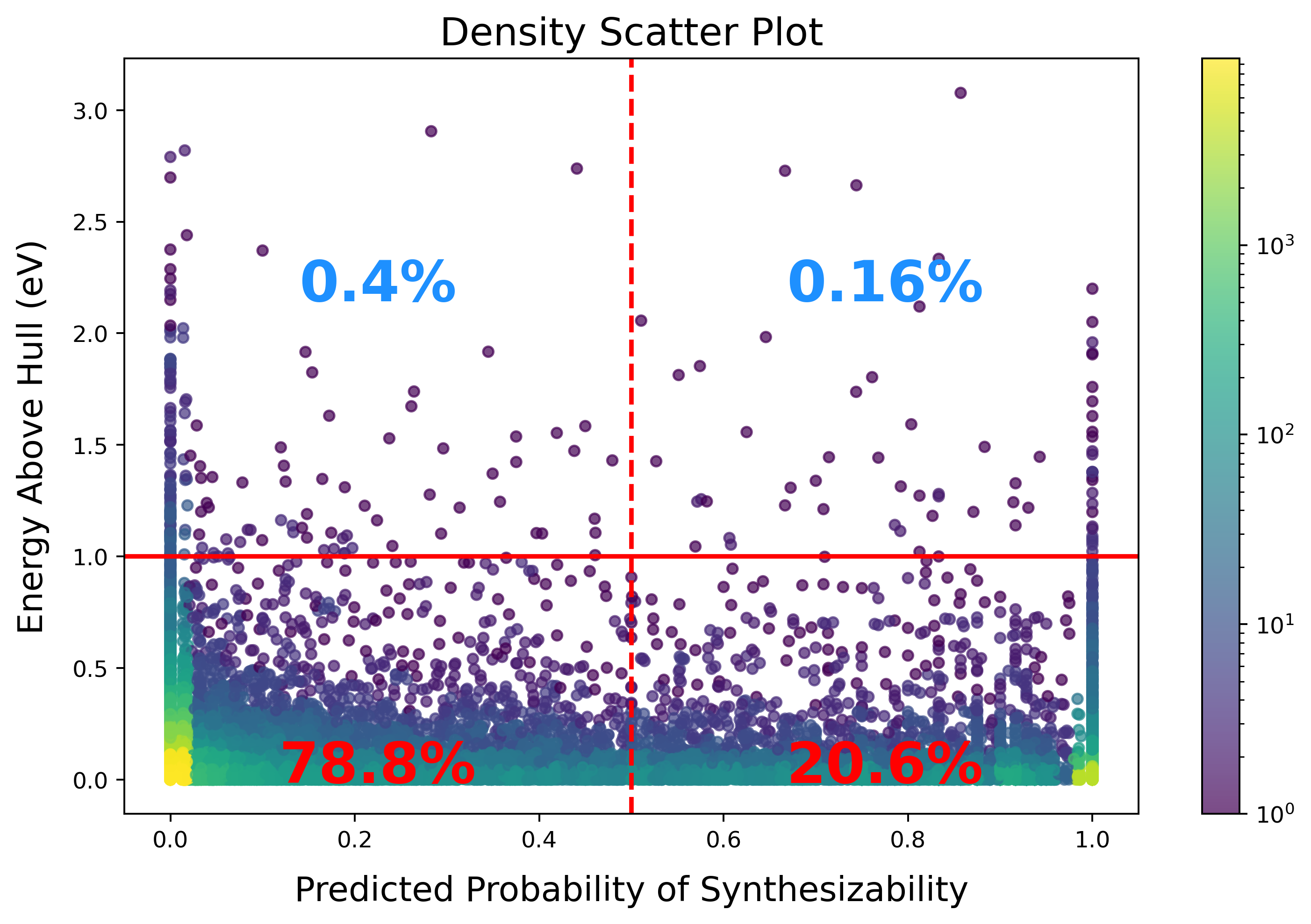
Next, we observe the synthesizability score for the unlabeled data and its relation to stability. Crystals with energy more than 1eV above the convex hull are quite unstable and highly unlikely to be synthesizable. As shown in Fig. 6 these unstable crystals are 2.5 times less likely to be classified synthesizable, as opposed to not-synthesizable. Also, more than 99% of the unlabeled crystals that are classified as synthesizable, have an energy less than 1eV above the convex hull. This shows that the model has captured the property of stability, even without having been specifically trained on it. On the other hand, among all the crystals with energy less than 1eV above hull, only about 21% are classified as synthesizable. This again indicates that while stability is a major contributor to synthesizability, it is not sufficient for predicting it. Of course, these observations are under the limitations of DFT such as finite temperature effects and precision.
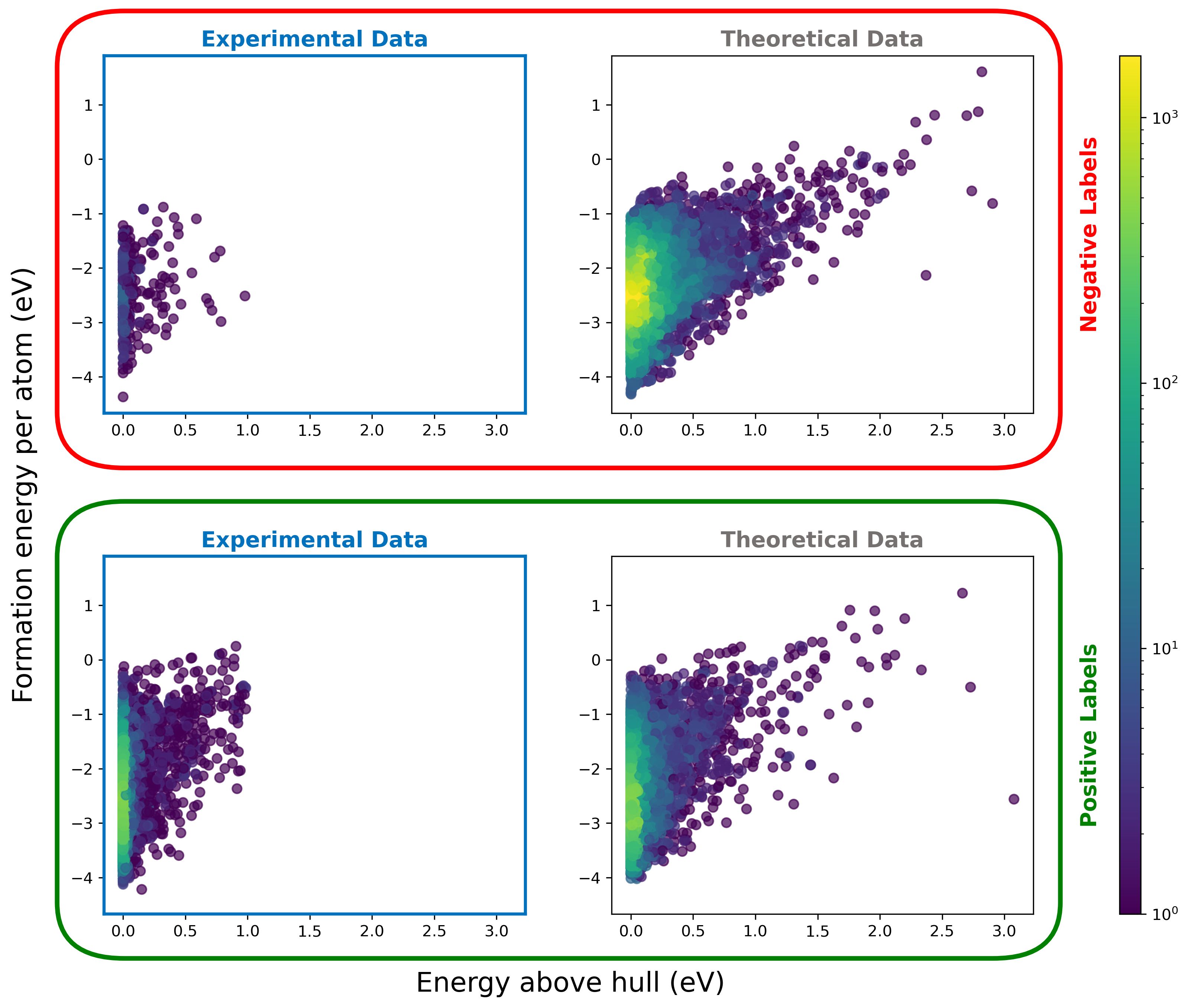
In Fig. 7 we compare the energy above hull and formation energy for data with positive and negative labels. Here, we find an expected clustering of positive data around lower values of energy above hull without any visible density peaks with regards to formation energy. This is expected, as stability (and by proxy synthesizability) depend on relative available energy states less than an absolute value. The column on the left is a measure of how trustworthy our model has been, as we know all the experimental data belongs to the positive class. The column on the right demonstrates the actual task of this ensemble, which is to separate the positive and negative classes within the unlabeled data.
2.3 Ground Truth evaluation
2.3.1 Test-sets construction
Construction of a suitable test-set is required to report any type error or merit measure in machine learning; more-so when predicting out-of-distribution data is concerned [25]. In their paper establishing the bagging PU Learning method [31], Mordelet and Vert use a different test-set at each run. After all runs have been executed, the average label predicted for each datum as part of the test-set is taken as the probability of it belonging to the positive class. A threshold is then applied to this probability to determine the label of the datum, and thus, the error criteria. This does not lead to ‘data leakage’ as no model is tested on the data it has been trained on. This dynamic test-set also lends itself well to co-training, as it does not take away valuable data permanently from the growing train-sets of further iterations.
On the other hand, using a leave-out test-set in the common practice in materials informatics. At the very least, a leave-out test-set would provide a more comparable evaluation with similar works in this topic.
Ultimately, the goal of a test error is to approximate the expected test error. By using both test sets, we will have two values for Recall. That means more information about the model’s performance. We chose a leave-out test set with 5% of the positive data for all the runs. For the dynamic test set, 10% of the positive data is chosen at each run of the PU learning.
2.3.2 Ground truth in PU learning
Recall is the typical measure for evaluating PU learning tasks. Due to the unlabeled data, this is not the most reliable measure. Recall only tells us how much of the known positive samples were classified correctly. The assumption is that the positive data are sampled from an unknown distribution. Hence, the Recall based on the labeled data should approximate a Recall based on all the positive data. Yet, it would be beneficial to have some evidence, even if qualitative, that the Recall solely based on the labeled data in fact approximates a Recall based on all the data, the Ground Truth Recall. To that end, we construct a new PU learning task with the goal of predicting classes of stability. As mentioned earlier, stability and synthesizability are related properties. If the recall values for labeled stability classes closely approximate the Ground Truth Recall for all of the data, this suggests a similar behavior in the recall values for synthesizability.
We use the same dataset as before, now including the outliers of experimental structures with high energy above hull that were previously excluded. This adjustment retains data for learning the higher energy structure and provides a better benchmark for comparison with previous works in synthesizability that used the outliers. These data points were classified into positive (stable) and negative (unstable) classes based on a cutoff in energy above the convex hull; for details please see supplementary materials. The key difference is that, unlike a real PU learning task, all the positive and negative labels are available for evaluation post training. A random subset of the positive class, with the same number of data points as the original experimental class, kept their positive label. We then hid the label of the remaining data to manufacture a PU learning scenario. The models were trained on the stability PU data using the same code as the synthesizability task. Having access to all the labels, we could estimate the Ground Truth Recall value and compare it with the Recall values produces by the two test sets.
As shown in Fig. 8, the recall values produced by both test-sets closely approximate the Ground Truth Recall, confirming the reliability of using Recall for evaluating the model’s performance. In both co-training series, the leave-out recall value starts more optimistic than the ground truth, especially when high-energy experimental outliers are included in the PU Learning. This optimistic recall was the reported recall value in the previous PU learning studies predicting synthesizability [14, 23]. From iteration ‘1’ of co-training the order flips and the dynamic test set becomes too optimistic. While there is no guarantee the ground-truth will always be found in the range between the two values, Fig. 8 illustrates why using both test-sets is worthwhile rather than just keeping one.
2.4 Predicting Synthesizability
The final step in this work involves training a synthesizability predictor using reliable labels generated through co-training. Since materials databases apply different criteria for data inclusion, they exhibit varied data distributions. Consequently, achieving optimal performance on a specific test set is insufficient. It is crucial to avoid bias toward the Materials Project data distribution, which was used to train the model. To mitigate this, we applied regularization techniques during training to prevent overfitting. This was not particularly important in the PU runs, where classifier instability enhances the bagging process by introducing variability [31]. In the final step, however, the model needs to generalize well to data distributions not seen during training, while still maintaining good performance on the test-set.
We selected SchNet as our classifier and achieved good results, though other classifiers like ALIGNN can also be trained using the same labels. Detailed training parameters are available in the METHODS section. The pretrained model is accessible in our repository https://github.com/BAMeScience/SynCoTrainMP).
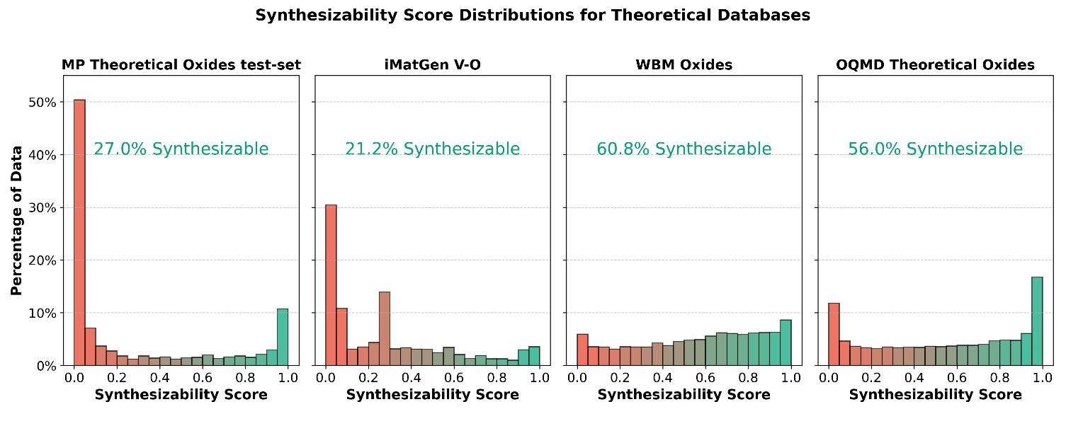
The trained model reached 90.5% accuracy on a test set comprising 5,180 data points. To further evaluate the model’s performance, we analyzed the synthesizability predictions for three additional datasets, focusing exclusively on oxides. First, we examined theoretical oxides from the Open Quantum Materials Database (OQMD) [36], downloaded via the Jarvis Python package [37], after filtering out any crystals already present in Materials Project’s experimental data, leaving 23,056 theoretical oxides. Second, we analyzed 14,095 oxide crystals from the WBM dataset [38], which were generated using random sampling of elements in Materials Project structures, with chemical similarity safeguards based on ICSD data [34]. We used the relaxed version of this dataset. Finally, we predicted the synthesizability of 6,156 vanadium oxide crystals generated by iMatGen [11]. Fig. 9 compares the synthesizability scores of these datasets with the theoretical portion of the test set. All These crystal structures and their predicted synthesizability scores are available to download in our GitHub repository.
Over half of the theoretical test-set data shows a synthesizability score close to zero, as expected, since previously synthesized crystals have been excluded by Materials Project. In contrast, the OQMD data shows roughly twice the proportion of synthesizable crystals, which may result from differing inclusion criteria between Materials Project and OQMD. We still observe a peak near a score of 1, possibly indicating synthesized crystals not listed in Materials Project. The iMatGen data show the lowest synthesizability, with multiple peaks at low scores, reflecting the artificial nature of these generated structures, which are often less realistic. The WBM dataset scores higher on average, without significant peaks. Despite being artificially generated, the WBM data employed mechanisms like chemical similarity to avoid unstable crystals. As a result, we observe more novel crystals with ambiguous synthesizability predictions, with scores around 0.5, and no clear peaks close to 0 or 1.
2.5 Discussion
In modern material discovery, the first challenge is the abundance of choices. The number of materials that may exist is astronomical [39] and high-throughput methods cannot screen them all. The nebulous nature of the synthesizability question makes the development of a flawless model challenging. The goal, however, is not perfection. Based on the findings of this and other related studies, the majority of the unlabeled data is determined to be unsynthesizable. Energy calculations, while important, are not a good proxy for synthesizability. Filtering out even half of the unsynthesizable data through synthesizability prediction could save a significant amount of resources on simulations and synthesis attempts. We imagine that our tool can be used in the initial stages of materials discovery, to filter out the structures which are not likely to result in real materials.
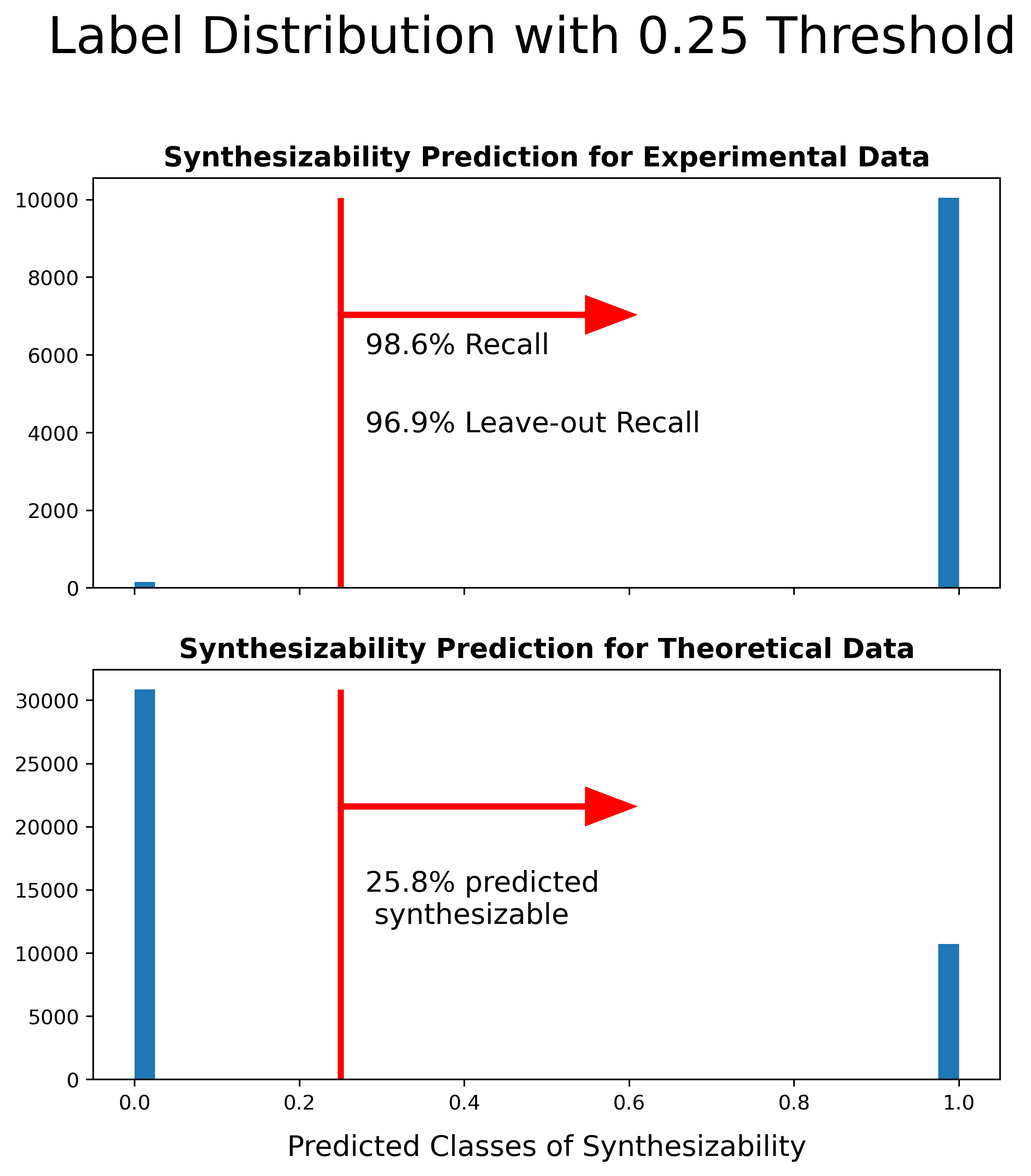
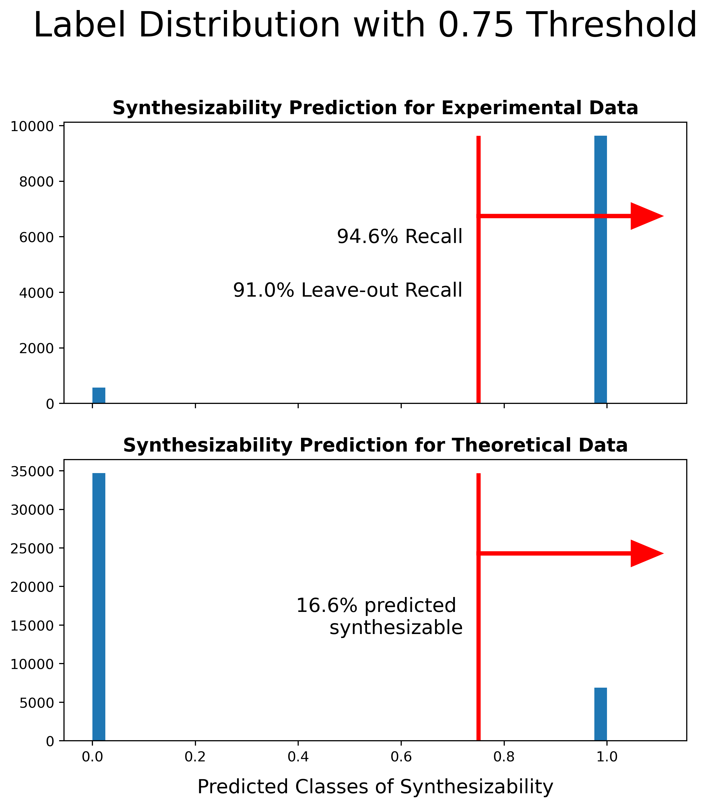
The decision thresholds of 0.5 and 0.75 were used as unbiased values for classification and class expansion. However, these thresholds are ultimately arbitrary and can be adjusted based on the specific goals and applications. In a more exploratory study, a looser threshold could be utilized to avoid overlooking potentially interesting novel structures. Conversely, a project operating with a tighter budget could employ a stricter threshold to save on resources. Label distributions based on a threshold of 0.25 and 0.75 are illustrated as examples in Fig. 10. When compared with the unbiased threshold of 0.5 shown in Fig. 5, a cutoff threshold of 0.25 is more lenient in classifying crystals as synthesizable. However, it only identifies 26% of the theoretical oxides in Materials Project as synthesizable, recognizing two thirds of the data as unsynthesizable. Conversely, a threshold of 0.75 results in a more stringent classification, with only 17% of the theoretical oxides meeting this threshold. And yet, these oxides are more likely to be synthesizable compared to those that did not meet the cut.
In this work we combined two different learners based on strong classifiers to reach a more reliable recall. New models for predicting materials properties are developed rapidly and materials data is growing. Combining different tools, instead creating one from scratch, is an untapped potential to learn more from the data already available in the materials space.
3 METHODS
3.1 Co-training
The co-training algorithm used here was based on previous work in [26, 27]. It is based on the idea that each data point can be described by distinct sets of descriptors, each of which are sufficient for learning the target. Consequently, two models learning from different views of the data can each gain knowledge that is inherently complementary. This is analogous to transfer learning; but the transfer happens between the knowledge gained from different views of the same data, rather than an auxiliary data source.
At each iteration, a base learner calculates a synthesizability score between 0 and 1 for both the unlabeled and experimental test data. To expand the positive class, unlabeled data points confidently classified as positive by the PU learner are selected. Here, we use a threshold of 0.75, rather than 0.5, to determine which unlabeled data points are added in the original positive class. After iteration ‘2’, the scores from both training series are averaged. The 0.5 cutoff determines the final label.
The base learner was changed from the original naïve Bayes classifier to a base PU learners equipped with convolutional neural networks. The different views of the data were achieved through the difference between the data encoding in the classifiers, i.e., ALIGNN and SchNet. Two parallel co-training series with altering classifiers were carried out accordingly.
3.2 PU Learning
The algorithm of PU learning was established by Mordelet and Vert [31]. This method treats the unlabeled data as negative data, contaminated with positive data. PU learning performs best when this contamination is low.
In this work, two base PU learners were made through using two classifiers. In both cases, a complete bagging of PU learning took 60 runs. Note that the separate runs of PU learning are not referred to as iterations as each run is independent of the rest. This is not the case in co-training, where each iteration depends on the results produced by the previous iteration.
The training data at each PU learning run has a 1:1 ratio of positive and negative labels. The size of the training set increases after each co-training iteration, due to the expansion of the positive class. Each run of PU learning predicts a label, 0 or 1, for the data points that did not take part in the training phase of that run. After the 60 runs, these predictions are averaged for each data to produce the synthesizability score. This score is also referred to as the predicted probability of synthesizability. The cutoff thresholds of 0.5 and 0.75 are used to predict the labels and expand the positive class, respectively.
3.3 Neural Networks architecture
The ALIGNN model was used according to instructions provided in its repository. We used the version 2023.10.01 of ALIGNN.
The SchNetPack model was originally designed for regression. To accommodate classification, a sigmoid non-linearity and a cutoff function were added to the final layer. We used the version 1.0.0.dev0 of this model.
3.4 The synthesizability predictor
The data labeling process utilized the averaged synthesizability scores produced in iteration ’2’ of co-training. A cutoff of 0.75 was applied for assigning positive labels, similar to the class expansion strategy, reducing the likelihood of training on uncertain labels.
During initial tests, the predictor displayed a tendency to overestimate the positive class, likely due to overfitting to the data distribution in the Materials Project. To mitigate this, several regularization steps were introduced. First, noise was added to the labels by randomly selecting 5% of the positive class and flipping their labels from 1 to 0. An equal number of negative class labels were also flipped from 0 to 1. This small amount of label noise helps regularize the model, preventing classifier’s overconfidence in any class distribution.
Data augmentation was then employed, following a previously published method that showed significant improvements in predicting material properties. This approach perturbs atomic positions using Gaussian noise to generate slightly altered versions of the original data, which are used alongside the unperturbed data for training. This augmentation doubles the size of the training set.
The SchNet model was used as the primary synthesizability predictor, with additional regularization techniques enhancing its generalizability. A weighted loss function was employed, with a ratio of 0.45:0.55 for the positive and negative classes, respectively. This adjustment subtly discouraged over-prediction of the positive class, while maintaining model sensitivity.
Finally, to implement regularization during training, dropout layers were added to the model, with 10% dropout at the embedding layer and 20% at each convolutional layer. To manage the learning rate, a ‘Cosine Annealing with Warm Restarts‘ scheduler was used, allowing it to cycle through phases, helping the model escape local minima early in training while converging effectively later on. Early stopping was also implemented to prevent overtraining.
3.5 Datasets
The experimental and theoretical data for co-training was queried from the Materials Project API [6], database version 2023.11.1.
4 DATA AVAILABILITY
The code for downloading the data used in this project, and the cleaned version of the data are available at https://github.com/BAMeScience/SynCoTrainMP.
5 CODE AVAILABILITY
The code used for training SynCoTrain and predicting synthesizability is available at https://github.com/BAMeScience/SynCoTrainMP.
References
- [1] De Pablo, J. J., Jackson, N. E., Webb, M. A., Chen, L.-Q., Moore, J. E., Morgan, D., Jacobs, R., Pollock, T., Schlom, D. G., Toberer, E. S., Analytis, J., Dabo, I., DeLongchamp, D. M., Fiete, G. A., Grason, G. M., Hautier, G., Mo, Y., Rajan, K., Reed, E. J., Rodriguez, E., Stevanovic, V., Suntivich, J., Thornton, K., and Zhao, J.-C. (April, 2019) New frontiers for the materials genome initiative. npj Computational Materials, 5(1), 41.
- [2] White, A. (August, 2012) The Materials Genome Initiative: One year on. MRS Bulletin, 37(8), 715–716.
- [3] Rodgers, J. R. and Cebon, D. (December, 2006) Materials Informatics. MRS Bulletin, 31(12), 975–980.
- [4] Pauling, L. (April, 1929) THE PRINCIPLES DETERMINING THE STRUCTURE OF COMPLEX IONIC CRYSTALS. Journal of the American Chemical Society, 51(4), 1010–1026 Publisher: American Chemical Society.
- [5] Antoniuk, E., Cheon, G., Wang, G., Bernstein, D., Cai, W., and Reed, E., Predicting the Synthesizability of Crystalline Inorganic Materials from the Data of Known Material Compositions. preprint, In Review (March, 2023).
- [6] Jain, A., Ong, S. P., Hautier, G., Chen, W., Richards, W. D., Dacek, S., Cholia, S., Gunter, D., Skinner, D., Ceder, G., and Persson, K. A. (July, 2013) Commentary: The Materials Project: A materials genome approach to accelerating materials innovation. APL Materials, 1(1), 011002 Publisher: American Institute of Physics.
- [7] George, J., Waroquiers, D., Di Stefano, D., Petretto, G., Rignanese, G., and Hautier, G. (May, 2020) The Limited Predictive Power of the Pauling Rules. Angewandte Chemie, 132(19), 7639–7645.
- [8] Sun, W., Dacek, S. T., Ong, S. P., Hautier, G., Jain, A., Richards, W. D., Gamst, A. C., Persson, K. A., and Ceder, G. (November, 2016) The thermodynamic scale of inorganic crystalline metastability. Science Advances, 2(11), e1600225.
- [9] Cerqueira, T. F. T., Lin, S., Amsler, M., Goedecker, S., Botti, S., and Marques, M. A. L. (July, 2015) Identification of Novel Cu, Ag, and Au Ternary Oxides from Global Structural Prediction. Chemistry of Materials, 27(13), 4562–4573 Publisher: American Chemical Society.
- [10] Singh, A. K., Montoya, J. H., Gregoire, J. M., and Persson, K. A. (January, 2019) Robust and synthesizable photocatalysts for CO2 reduction: a data-driven materials discovery. Nature Communications, 10(1), 443.
- [11] Noh, J., Kim, J., Stein, H. S., Sanchez-Lengeling, B., Gregoire, J. M., Aspuru-Guzik, A., and Jung, Y. (November, 2019) Inverse Design of Solid-State Materials via a Continuous Representation. Matter, 1(5), 1370–1384.
- [12] Wu, Y., Lazic, P., Hautier, G., Persson, K., and Ceder, G. (December, 2012) First principles high throughput screening of oxynitrides for water-splitting photocatalysts. Energy & Environmental Science, 6(1), 157–168 Publisher: The Royal Society of Chemistry.
- [13] Bartel, C. J. (February, 2022) Review of computational approaches to predict the thermodynamic stability of inorganic solids. Journal of Materials Science,.
- [14] Jang, J., Gu, G. H., Noh, J., Kim, J., and Jung, Y. (November, 2020) Structure-Based Synthesizability Prediction of Crystals Using Partially Supervised Learning. Journal of the American Chemical Society, 142(44), 18836–18843.
- [15] Lee, A., Sarker, S., Saal, J. E., Ward, L., Borg, C., Mehta, A., and Wolverton, C. (October, 2022) Machine learned synthesizability predictions aided by density functional theory. Communications Materials, 3(1), 73.
- [16] Li, K. and Chen, W. (June, 2021) Recent progress in high-entropy alloys for catalysts: synthesis, applications, and prospects. Materials Today Energy, 20, 100638.
- [17] Miao, M., Sun, Y., Zurek, E., and Lin, H. (October, 2020) Chemistry under high pressure. Nature Reviews Chemistry, 4(10), 508–527 Publisher: Nature Publishing Group.
- [18] Liu, C., Gao, H., Hermann, A., Wang, Y., Miao, M., Pickard, C. J., Needs, R. J., Wang, H.-T., Xing, D., and Sun, J. (April, 2020) Plastic and Superionic Helium Ammonia Compounds under High Pressure and High Temperature. Physical Review X, 10(2), 021007.
- [19] Legrain, F., Carrete, J., van Roekeghem, A., Madsen, G. K., and Mingo, N. (January, 2018) Materials Screening for the Discovery of New Half-Heuslers: Machine Learning versus ab Initio Methods. The Journal of Physical Chemistry B, 122(2), 625–632 Publisher: American Chemical Society.
- [20] Huo, H., Rong, Z., Kononova, O., Sun, W., Botari, T., He, T., Tshitoyan, V., and Ceder, G. (July, 2019) Semi-supervised machine-learning classification of materials synthesis procedures. npj Computational Materials, 5(1), 62.
- [21] Davariashtiyani, A., Kadkhodaie, Z., and Kadkhodaei, S. (December, 2021) Predicting synthesizability of crystalline materials via deep learning. Communications Materials, 2(1), 115.
- [22] Aykol, M., Hegde, V. I., Hung, L., Suram, S., Herring, P., Wolverton, C., and Hummelshøj, J. S. (May, 2019) Network analysis of synthesizable materials discovery. Nature Communications, 10(1), 2018.
- [23] Gu, G. H., Jang, J., Noh, J., Walsh, A., and Jung, Y. (April, 2022) Perovskite synthesizability using graph neural networks. npj Computational Materials, 8(1), 71.
- [24] Raccuglia, P., Elbert, K. C., Adler, P. D. F., Falk, C., Wenny, M. B., Mollo, A., Zeller, M., Friedler, S. A., Schrier, J., and Norquist, A. J. (May, 2016) Machine-learning-assisted materials discovery using failed experiments. Nature, 533(7601), 73–76.
- [25] Li, K., DeCost, B., Choudhary, K., Greenwood, M., and Hattrick-Simpers, J. (April, 2023) A critical examination of robustness and generalizability of machine learning prediction of materials properties. npj Computational Materials, 9(1), 1–9 Number: 1 Publisher: Nature Publishing Group.
- [26] Blum, A. and Mitchell, T. (July, 1998) Combining labeled and unlabeled data with co-training. In Proceedings of the eleventh annual conference on Computational learning theory Madison Wisconsin USA: ACM pp. 92–100.
- [27] Denis, F., Laurent, A., Gilleron, R., and Tommasi, M. (2003) Text Classification and Co-training from Positive and Unlabeled Examples. Proceedings of the ICML 2003 workshop: the continuum from labeled to unlabeled data, p. 8.
- [28] Choudhary, K. and DeCost, B. (November, 2021) Atomistic Line Graph Neural Network for improved materials property predictions. npj Computational Materials, 7(1), 185.
- [29] Schütt, K. T., Kessel, P., Gastegger, M., Nicoli, K. A., Tkatchenko, A., and Müller, K.-R. (January, 2019) SchNetPack: A Deep Learning Toolbox For Atomistic Systems. Journal of Chemical Theory and Computation, 15(1), 448–455.
- [30] Schütt, K. T., Kindermans, P.-J., Sauceda, H. E., Chmiela, S., Tkatchenko, A., and Müller, K.-R. (December, 2017) SchNet: A continuous-filter convolutional neural network for modeling quantum interactions. arXiv:1706.08566 [physics, stat], arXiv: 1706.08566.
- [31] Mordelet, F. and Vert, J.-P. (February, 2014) A bagging SVM to learn from positive and unlabeled examples. Pattern Recognition Letters, 37, 201–209.
- [32] Savkina, R. and Khomenkova, L. (May, 2020) Oxide-Based Materials and Structures: Fundamentals and Applications, CRC Press, Google-Books-ID: Q7XjDwAAQBAJ.
- [33] Waroquiers, D., Gonze, X., Rignanese, G.-M., Welker-Nieuwoudt, C., Rosowski, F., Göbel, M., Schenk, S., Degelmann, P., André, R., Glaum, R., and Hautier, G. (October, 2017) Statistical Analysis of Coordination Environments in Oxides. Chemistry of Materials, 29(19), 8346–8360.
- [34] Hellenbrandt, M. (2004) The Inorganic Crystal Structure Database (ICSD)—Present and Future. Crystallography Reviews, 10(1), 17–22.
- [35] Ong, S. P., Richards, W. D., Jain, A., Hautier, G., Kocher, M., Cholia, S., Gunter, D., Chevrier, V. L., Persson, K. A., and Ceder, G. (February, 2013) Python Materials Genomics (pymatgen): A robust, open-source python library for materials analysis. Computational Materials Science, 68, 314–319.
- [36] Kirklin, S., Saal, J. E., Meredig, B., Thompson, A., Doak, J. W., Aykol, M., Rühl, S., and Wolverton, C. (December, 2015) The Open Quantum Materials Database (OQMD): assessing the accuracy of DFT formation energies. npj Computational Materials, 1(1), 15010.
- [37] Choudhary, K., Garrity, K. F., Reid, A. C. E., DeCost, B., Biacchi, A. J., Hight Walker, A. R., Trautt, Z., Hattrick-Simpers, J., Kusne, A. G., Centrone, A., Davydov, A., Jiang, J., Pachter, R., Cheon, G., Reed, E., Agrawal, A., Qian, X., Sharma, V., Zhuang, H., Kalinin, S. V., Sumpter, B. G., Pilania, G., Acar, P., Mandal, S., Haule, K., Vanderbilt, D., Rabe, K., and Tavazza, F. (November, 2020) The joint automated repository for various integrated simulations (JARVIS) for data-driven materials design. npj Computational Materials, 6(1), 173.
- [38] Wang, H.-C., Botti, S., and Marques, M. A. L. (January, 2021) Predicting stable crystalline compounds using chemical similarity. npj Computational Materials, 7(1), 1–9 Publisher: Nature Publishing Group.
- [39] Davies, D., Butler, K., Jackson, A., Morris, A., Frost, J., Skelton, J., and Walsh, A. (October, 2016) Computational Screening of All Stoichiometric Inorganic Materials. Chem, 1(4), 617–627.
- [40] Riebesell, J., Goodall, R., Benner, P., Chiang, Y., Deng, B., Lee, A., Jain, A., and Persson, K. Matbench Discovery: An evaluation framework for machine learning crystal stability prediction. (August, 2023) Available at: https://janosh.github.io/matbench-discovery.
- [41] Matbench Discovery v1.0.0. (April, 2023) Available at: https://figshare.com/articles/dataset/Matbench_Discovery_v1_0_0/22715158/13.