Using LSTM Predictions for RANS Simulations

This study constitutes the second phase of a research endeavor aimed at evaluating the feasibility of employing Long Short-Term Memory (LSTM) neural networks as a replacement for Reynolds-Averaged Navier-Stokes (RANS) turbulence models.

In the initial phase of this investigation (titled Modeling Turbulent Flows with LSTM Neural Networks, arXiv:2307.13784v1 [physics.flu-dyn] 25 Jul 2023), the application of an LSTM-based recurrent neural network (RNN) as an alternative to traditional RANS models was demonstrated. LSTM models were used to predict shear Reynolds stresses in both developed and developing turbulent channel flows, and these predictions were propagated through RANS simulations to obtain mean flow fields of turbulent flows. A comparative analysis was conducted, juxtaposing the LSTM results from computational fluid dynamics (CFD) simulations with outcomes from the $\kappa-\epsilon$ model and data from direct numerical simulations (DNS). These initial findings indicated promising performance of the LSTM approach.

This second phase delves further into the challenges encountered and presents robust solutions. Additionally, new results are provided, demonstrating the efficacy of the LSTM model in predicting turbulent behavior in perturbed flows. While the overall study serves as a proof-of-concept for the application of LSTM networks in RANS turbulence modeling, this phase offers compelling evidence of its potential in handling more complex flow scenarios.

Keywords LSTM neural networks; Turbulent flow modeling; RANS simulations

1 Introduction

The objective of this research is to investigate the use of Recurrent Neural Networks (RNNs), specifically Long Short-Term Memory (LSTM) models, as a substitute for traditional turbulence models within the framework of Reynolds-averaged Navier-Stokes (RANS) equations Pope (2000). These equations, expressed in dimensionless form using tensor notation, represent the conservation of mass:

$$\frac{\partial U_{i}}{\partial x_{i}}=0,$$ (1)

and the momentum equations:

$$\frac{\partial U_{i}}{\partial t}+\frac{\partial(U_{j}U_{i})}{\partial x_{j}}=-\frac{\partial P}{\partial x_{i}}+\frac{1}{Re_{\tau}}\frac{\partial^{2}U_{i}}{\partial x_{j}\partial x_{j}}-\frac{\partial\langle u_{j}u_{i}\rangle}{\partial x_{j}},$$ (2)

where $U_{i}$ (corresponding to $U$, $V$, and $W$) represents the mean velocity, $P$ the mean pressure, and $x$ and $t$ are the spatial and temporal coordinates, respectively. The friction Reynolds number, $Re_{\tau}$, is defined as $u_{\tau}\delta/\nu$, where all variables are non-dimensionalized using the friction velocity $u_{\tau}$ and half the distance between the walls $\delta$, serving as the characteristic velocity and length scales.

The last term on the right-hand side of equation (2) is the Reynolds stress tensor $\langle u_{j}u_{i}\rangle$, which arises from time-averaging the original Navier-Stokes equations and introduces new unknowns into the system. Since the Reynolds stress tensor is symmetric, solving the RANS equations necessitates addressing six additional unknowns, alongside the velocity components $U_{i}$ and the pressure $P$.

To resolve the RANS equations, a method for determining these six unknowns must be incorporated, as they are needed to compute the velocities $U$, $V$, and $W$, along with the pressure $P$, derived from the conservation equations of momentum and mass. These methods are collectively referred to as RANS turbulence modeling, with the Kappa-Epsilon model being a well-known example. Such models typically employ a pseudo viscosity that accounts for the effects of turbulence, drawing an analogy between the behavior of a Newtonian fluid and a turbulent flow. By incorporating this pseudo viscosity, these models aim to replicate the dynamics of turbulent flows in a manner similar to the behavior of Newtonian fluids.

The current study aims to replace the turbulence model within the RANS framework with an LSTM-based recurrent neural network. In a previous preprint Pasinato (2023), the fundamental concepts of this approach and initial results were presented. This preprint provides a detailed description of how the LSTM’s predictions are propagated. The following sections outline the architecture of the LSTM models employed in the study (§2), followed by a description of the DNS data used for model training and adjustments (§3). Numerical details of the RANS simulations are provided in §4, while the results are presented in §5, with conclusions drawn in §6.

2 LSTM Models

One architecture of LSTM RNN is the sequence-by-sequence (seqxseq) architecture. In this format, a sequence in time of input-output pairs is trained (Hochriter and Schmidhuber (1997); Sutskever et al. (2014)). However, to apply this architecture within RANS simulations, a fundamental adaptation was necessary. Most turbulent flows analyzed in RANS simulations are statistically stationary, meaning the Reynolds-averaged values along the x-direction at a constant distance from the boundary form a spatial sequence—from upstream to downstream—. Therefore, in this study, the LSTM neural network was trained using spatial sequence-by-sequence data instead of time-based sequences, as explained in the first part of the study (Pasinato (2023)). Each sequence comprised 32 consecutive input-output pairs corresponding to nodes in the RANS simulations along the longitudinal direction, spanning the entire physical domain. The data were normalized between 0 and 1, using the global maximum and minimum values from the dataset.

Once the Reynolds shear stresses are predicted, new challenges arise regarding their integration into the RANS simulations. One of the key difficulties in employing neural networks to predict Reynolds stresses in RANS simulations lies in how these turbulent stress values are incorporated into computational fluid dynamics (CFD) codes to produce a robust solution for turbulent flow. While neural networks trained on Direct Numerical Simulation (DNS) databases can accurately predict Reynolds stresses, improvements in mean flow fields are not guaranteed, as highlighted by Wu et al. (2019). Wu and colleagues explored potential ill-conditioning of the RANS equations when explicit Reynolds stresses are included in mean velocity calculations. Even when DNS-derived Reynolds stresses are used in RANS simulations at high Reynolds numbers, significant errors in velocity predictions can still occur Thompson et al. (2016).

Although the present study focuses on turbulent flows at moderately low Reynolds numbers, addressing the explicit incorporation of stresses into the RANS equations required consideration of two key aspects to develop robust predictions. First, it was acknowledged that the fragility of neural networks often correlates with their capacity, defined by the number of parameters. Thus, the initial step involved reducing the number of parameters without risking underfitting—essentially, designing a parsimonious LSTM model. Striking the right balance between complexity and simplicity was essential, ensuring that only the necessary parameters were included to adequately represent the phenomena, thereby avoiding unnecessary redundancy or overfitting.

The second aspect involved the use of bidirectional wrapping architectures. As previously noted, turbulence is not a local phenomenon; the transport of momentum by turbulence at a given point in space depends on the flow characteristics both upstream and downstream of this point. Therefore, based on prior experience, a strategy to improve the stability of using explicit Reynolds stresses in the RANS equations involved employing LSTM models with bidirectional wrapping architectures.

Name	Stacked LSTM	Parameters	Features	Prediction
1XL110DL	0	491	$S_{12}^{+}$	$\langle uv\rangle^{+}$
2XL120DL	0	1861	$S_{12}^{+};Y$	$\langle uv\rangle^{+}$
2XBL13BL23BL33DL	3	631	$S_{12}^{+};Y$	$\langle uv\rangle^{+}$
3XBL13BL23BL33DL	3	655	$S_{12}^{+};Y;Re_{\tau}$	$\langle uv\rangle^{+}$
4XBL13BL23BL33DL	3	679	$Re_{\tau};S_{11}^{+};S_{12}^{+};Y$	$\langle uv\rangle^{+}$
4XBL14BL24DL	3	713	$Re_{\tau};S_{11}^{+};S_{12}^{+};Y$	$\langle uv\rangle^{+}$
5XBL13BL23BL33DL	3	703	$Re_{\tau};S_{11}^{+};S_{12}^{+};S_{22}^{+};Y$	$\langle uv\rangle^{+}$

Table 1: LSTM models.

Table 1 presents some of the LSTM architectures employed in the second phase of this study. For example, $4XBL13BL23BL33DL$ denotes an LSTM model with an input vector comprising four features and three stacked LSTM layers, each with three memory units and bidirectional wrapping, and a dense layer at the output. The features $S_{11}^{+}$, etc., represent components of the dimensionless mean rate-of-strain tensor $S_{ij}$, calculated as $S_{ij}^{+}=({1}/{2})\left({\partial U^{+}_{i}}/{\partial x^{+}_{j}}+{\partial U^{+}_{j}}/{\partial x^{+}_{i}}\right)$. Additionally, $Y$ and $Re_{\tau}={u_{\tau}\delta\rho}/{\mu}$ denote the dimensionless wall distance ($y/\delta$) and the friction Reynolds number, respectively. It is important to note that the axes in $S_{ij}$ are non-dimensionalized differently from the wall distance $Y$.

The LSTM model, like other deep learning models, involves three primary hyperparameters: (a) the number of stacked layers (or stacked LSTM cells), (b) the number of memory units in each LSTM layer, and (c) the learning rate. These hyperparameters were selected in this study through trial and error.

As discussed in Pasinato (2023), another critical aspect of a neural network model is its universality. The appropriate balance between universality and simplicity must be addressed—how specialized and simple the model can be while maintaining performance. Developing a fully universal NN model would require a large number of adjustable parameters to capture all possible flow characteristics. However, fine-tuning such a model poses significant challenges, and integrating a neural network with a high parameter count into CFD software demands substantial computational resources. Therefore, this study sought to employ an RNN with a reduced parameter count to facilitate rapid predictions within a RANS simulation.

At this stage, the computational time of CFD simulations using an LSTM network was not the primary focus. The main objective was to develop an effective tool to replace traditional RANS turbulence models with a neural network. For comparison purposes, the computational time of a standard CFD simulation using the $\kappa-\epsilon$ model Pope (2000) was used as a reference. The goal was to employ LSTM architectures with no more than approximately 700 parameters, as LSTM models with this parameter count take approximately the same computational time as the $\kappa-\epsilon$ model. Although the LSTM model allows for larger time steps, each time step of the $\kappa-\epsilon$ model remains faster than those of the LSTM model.

In the second phase of this research, all software required for tuning the LSTM parameters was developed in Python using the Keras-TensorFlow libraries Abadi et al. (2015); Brownlee (2017). The LSTMforRANS repository, available on GitHub at (https://github.com/hugodariopasinato/LSTM-for-RANS), contains essential resources including the LSTM neural network model 4XBL13BL23BL33DL, the maxima and minima from the DNS dataset, and FORTRAN subroutines designed to load the LSTM model and use it for predictions. These subroutines can be integrated into CFD codes to enable RANS simulations incorporating LSTM-based predictions of Reynolds stress.

3 Training, testing, and validation data

Name	$Re_{\tau}$	Perturbation	Parameter	Purpose
Developed	150; 300; 600			training
Developed	200			validation
B1506	150	Blowing	$v^{+}=0.6$	training
S1506	150	Suction	$v^{+}=0.6$	training
APGS30025	300	APGS	$\partial P^{+}/\partial x^{+}=+0.25$	training
FPGS30025	300	FPGS	$\partial P^{+}/\partial x^{+}=-0.25$	training
WF150	150	Frictionless wall		validation
WF300	300	Frictionless wall		validation
WFB3003	300	Frictionless wall/Blowing	$v^{+}=0.3$	validation
WFAPGS15020	150	Frictionless wall/APGS	$\partial P^{+}/\partial x^{+}=+0.20$	validation
WFAPGS20025	200	Frictionless wall/APGS	$\partial P^{+}/\partial x^{+}=+0.25$	validation
WFFPGS20025	200	Frictionless wall/APGS	$\partial P^{+}/\partial x^{+}=-0.25$	validation
WFFPGS30010	300	Frictionless wall/APGS	$\partial P^{+}/\partial x^{+}=-0.10$	validation
WFAPGS30010	300	Frictionless wall/APGS	$\partial P^{+}/\partial x^{+}=-0.10$	validation
WFS3003	300	Frictionless wall/Suction	$v^{+}=0.3$	validation
BS1503	150	Blowing/Suction	$v^{+}=0.3$	validation
SB3003	300	Suction/Blowing	$v^{+}=0.3$	validation

Table 2: Dataset used for training, testing, or validation purposes. $v^{+}$ represents the dimensionless wall-normal velocity at the wall for blowing or suction; $\partial P^{+}/\partial x^{+}$ denotes the pressure gradient step. ”APGS” and ”FPGS” refer to adverse and favorable pressure gradient steps, respectively. ”WFAPGS” and ”WFFPGS” refer to frictionless walls combined with APGS or FPGS. ”BS” represents blowing followed by suction, and ”SB” represents the reverse.

The DNS database of turbulent flows used for training, testing, and validation in this study was generated using a DNS numerical code that solves the incompressible momentum equations. These equations were discretized using a second-order accurate central-difference scheme. The Poisson equation for the pressure field was Fourier-transformed along the streamwise and spanwise directions, and the resulting tridiagonal systems were solved directly at each time step. The flow field evolution was computed using a fractional-step method, with the Crank-Nicolson second-order scheme applied to viscous terms, and the Adams-Bashforth scheme to non-linear terms. Further numerical details on the DNS calculations are available in Pasinato (2012) and Pasinato (2014).

The dataset consists of statistically stationary 2D turbulent channel flows at moderately low Reynolds numbers, which serves as a proof-of-concept for the application of LSTM networks in RANS turbulence modeling. The dataset includes developed turbulent channel flows for friction Reynolds numbers, $R_{\tau}$, of 150, 200, 300, and 600. The minimum friction Reynolds number in this study, $Re_{\tau}=150$, corresponds to $Re_{\delta}\simeq 2900$, where $Re_{\delta}=U2\delta/\nu\simeq(Re_{\tau}/0.1406)^{(8/7)}$, with $U$ being the mean velocity (where the $Re_{\delta,crit}\simeq 1400$). Additionally, the dataset includes perturbed channel flows subjected to wall blowing or suction, adverse (APGS) or favorable pressure gradient steps (FPGS), changes in wall friction (WF), and combinations of these perturbations, for $R_{\tau}$ values of 150, 200, 300, and 600. Table 2 provides a detailed list of these flows, including perturbation parameters and their respective purposes.

For instance, the case ”WFB3003” represents a turbulent flow initially developed with $R_{\tau}=300$ that is perturbed in a narrow region of width $W^{+}=206$ by wall blowing combined with a frictionless wall. In contrast, the case ”BS2003” refers to a flow initially developed with $R_{\tau}=200$, which is perturbed in two contiguous regions of width $W^{+}=206$ by blowing followed by suction, with $v^{+}=0.3$, resulting in a total perturbation region of $W^{+}=412$.

To understand the turbulence transport mechanisms in these perturbed cases in a RANS simulation, it is important to examine the impact on longitudinal momentum transport (x-direction). The transport of longitudinal momentum between the central region and the wall, which in a perturbed flow occurs via mean convection, turbulent flux, and molecular viscosity, is altered from the developed flow conditions. In developed flows, momentum transport towards the wall is driven primarily by the Reynolds stress, $\langle uv\rangle$, with no mean convection towards or away from the wall, and molecular viscosity becoming significant only in the near-wall region.

Each type of perturbation modifies the transport of longitudinal momentum between the central region and the wall. Perturbations such as blowing, suction, pressure gradient steps, and changes in wall friction modify $\langle uv\rangle$ and introduce mean convection towards or away from the wall. When a perturbation disrupts natural turbulent momentum transport, turbulence either intensifies or weakens, depending on whether the perturbation aids or opposes the momentum transfer.

In cases where perturbations introduce mean wall-normal convection that opposes turbulent fluxes (e.g., blowing, adverse pressure gradients, or increased wall friction), turbulence intensifies to compensate for the momentum deficit near the wall. Conversely, when perturbations assist momentum transport towards the wall (e.g., suction, favorable pressure gradients, or reduced wall friction), turbulent transport decreases. A well-known example is the relaminarization that occurs when a strong favorable pressure gradient is applied to a previously developed turbulent flow.

For validation purposes, the types and parameters of perturbations were adjusted. In the training flows, pressure gradient steps were introduced in the buffer region, whereas in the validation cases, they were applied in the logarithmic region. In both scenarios, the perturbations were confined to a narrow longitudinal region of width $W^{+}=206$. The combination of multiple perturbations can also significantly alter turbulent behavior. For example, a favorable pressure gradient step, which increases skin friction by drawing fluid towards the wall, behaves differently when applied alongside a frictionless wall. Similarly, combining blowing and suction leads to distinct effects compared to applying them individually. A suction region followed by a blowing region, for instance, induces sharp curvature in the mean flow streamlines, producing patterns that differ from those caused by either perturbation alone.

Future studies will require the development of new turbulent flows under varied boundary conditions and at higher Reynolds numbers to achieve more comprehensive validation. However, to ensure practical applicability in CFD codes, it is crucial to focus on developing neural networks tailored to specific types of turbulence, rather than pursuing universal models.

As described in Table 2, the ”training data” consists of DNS data used to adjust the LSTM model parameters. This data is further split into ”training” (80%) and ”testing” (20%) subsets during the training process. The ”validation data” refers to new DNS data used exclusively to compare DNS results with RANS simulations where LSTM predictions were incorporated.

4 Numerical Details of RANS Simulations

Each RANS simulation of perturbed turbulent flow (mirroring the approach used in the DNS simulations of perturbed flow) was conducted with two parallel simulations. Both simulations represent channel flow with the same $Re_{\tau}$, physical domain, and grid. The first simulation, using periodic boundary conditions, provided the inlet boundary conditions for the second simulation. This second simulation, which includes the perturbed (developing) flow, used the developed turbulent flow from the first simulation as its inlet condition, while convection boundary conditions were applied at the outlet. The width of the perturbation region, or slot, was fixed at $W^{+}=206$ for all cases, and the distance from the inlet to the perturbation region was approximately $X^{+}\simeq 600$. In cases where blowing was combined with suction (or vice versa), the total perturbation width was doubled, reaching $2W^{+}=412$.

All RANS simulations, both for the $\kappa-\epsilon$ model and for LSTM propagation, were conducted using the same computational domain and grid, with the only difference being the time step. The $\kappa-\epsilon$ model required a time step four times smaller than that used for the LSTM’s prediction propagation, due to the constraints imposed by solving the $\kappa$ and $\epsilon$ conservation equations numerically.

Both LSTM propagation and the $\kappa-\epsilon$ simulations were carried out within a physical domain scaled according to the $Re_{\tau}$ number. For example, at $Re_{\tau}=150$, the computational domain was $4\pi\delta\times 2\delta\times\frac{4}{3}\pi\delta$. For higher Reynolds numbers, this domain was adjusted accordingly. All RANS results presented here used a numerical grid of $32\times 32\times 32$, although a finer grid of $64\times 64\times 64$ was also tested. To employ a $64\times 64\times 64$ grid, an LSTM with sequences of 64 elements would be required; using an LSTM with sequences of only 32 elements on a grid of 64 nodes can lead to inconsistencies at grid junctions. For $Re_{\tau}=150$, the grid resolution was $\Delta x^{+}=88$, $\Delta z^{+}=39.2$, $\Delta y^{+}_{max}=52.8$, and $\Delta y^{+}_{min}=3$. A non-uniform mesh, distributed using a hyperbolic tangent function in the wall-normal direction, ensured that the $y^{+}$ value at the first cell center remained below 3. Near the wall, a van Driest damping function was applied with the $\kappa-\epsilon$ model. Given the low Reynolds number flows considered in this study, this wall-modeling approach is deemed appropriate.

5 Results

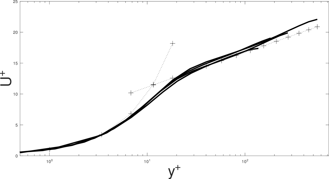
Figure 1: Dimensionless longitudinal velocity $U^{+}$ for various Reynolds numbers ($Re_{\tau}=150$, $200$, $300$, $600$) predicted by the LSTM model for developed channel flows. Solid line: LSTM; $+\cdot+\cdot+$, Law of the Wall, $U^{+}=({1}/{0.41})\ln(y^{+})+5.5$.

Figure 2: Shear Reynolds stresses predicted by the LSTM model for a developed channel flow with $Re_{\tau}=200$. $\diamond\cdot\diamond\cdot\diamond$Total; $\circ\cdot\circ\cdot\circ\;$Molecular; $\Box\cdot\Box\cdot\Box$ $\langle uv\rangle^{+}$; filled $\Box\cdot\Box\cdot\Box$ $\langle uv\rangle^{+}$ for $Re_{\tau}=600$ (using the same $y^{+}$ scale as for $Re_{\tau}=200$).

The LSTM models used in this study predict only the $\langle uv\rangle$ component of the Reynolds stress tensor. Therefore, in the RANS simulations where LSTM predictions are propagated, all other Reynolds stress components are set to zero. In general 3D turbulent flows, the Reynolds stresses, which result from time-averaging the Navier-Stokes equations, form a 9-component tensor. Since this tensor is symmetric, only six independent components need to be calculated by a RANS turbulence model. These include three normal stresses: $\langle uu\rangle$, $\langle vv\rangle$, and $\langle ww\rangle$, which represent turbulent flux transport in the x, y, and z directions, respectively. The remaining three components are shear stresses: $\langle uv\rangle$, $\langle uw\rangle$, and $\langle vw\rangle$, which are off-diagonal components of the tensor. Specifically, $\langle uv\rangle$ governs the turbulent transport of x-direction momentum in the y-direction, $\langle vw\rangle$ governs y-direction momentum in the z-direction, and $\langle uw\rangle$ governs z-direction momentum in the x-direction.

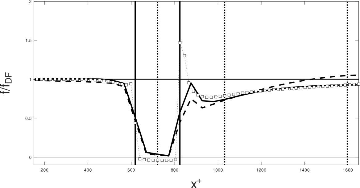
Figure 3: Normalized skin-friction coefficient $f/f_{DF}$ for a channel flow with $Re_{\tau}=200$, perturbed by a frictionless wall and an adverse pressure gradient step in a narrow region of width $W^{+}=206$. Solid vertical lines indicate the boundaries of the perturbation region, while dashed vertical lines represent its center and at distances of $W^{+}$ and $5W^{+}$ from its end. $---$, $\kappa-\epsilon$ model; $\Box\cdot\Box\cdot\Box$ , DNS; solid line, LSTM.

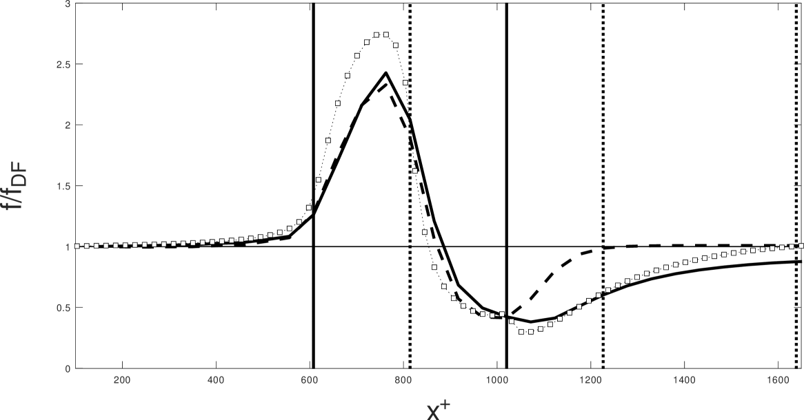
Figure 4: Normalized skin-friction coefficient $f/f_{DF}$ for a channel flow with $Re_{\tau}=300$, perturbed by wall suction followed by blowing in adjacent regions, each with a width of $W^{+}=206$, for a total perturbation width of $W^{+}=412$. $---$, $\kappa-\epsilon$ model; $\Box\cdot\Box\cdot\Box$ , DNS; solid line, LSTM.

Since the turbulent flows analyzed in this study are symmetric in the z-direction, they are treated as two-dimensional statistical turbulent flows. As a result, the only significant shear stress is $\langle uv\rangle$, which describes the transfer of momentum in the x-direction from the channel’s central region (higher momentum) toward the wall (lower momentum). The normal stresses are considered not relevant in this context and are set to zero to simplify the LSTM model. Consequently, the LSTM model is designed to predict and propagate only the $\langle uv\rangle$ shear stress. In contrast, the $\kappa-\epsilon$ model accounts for all Reynolds stresses, with none assumed to be zero.

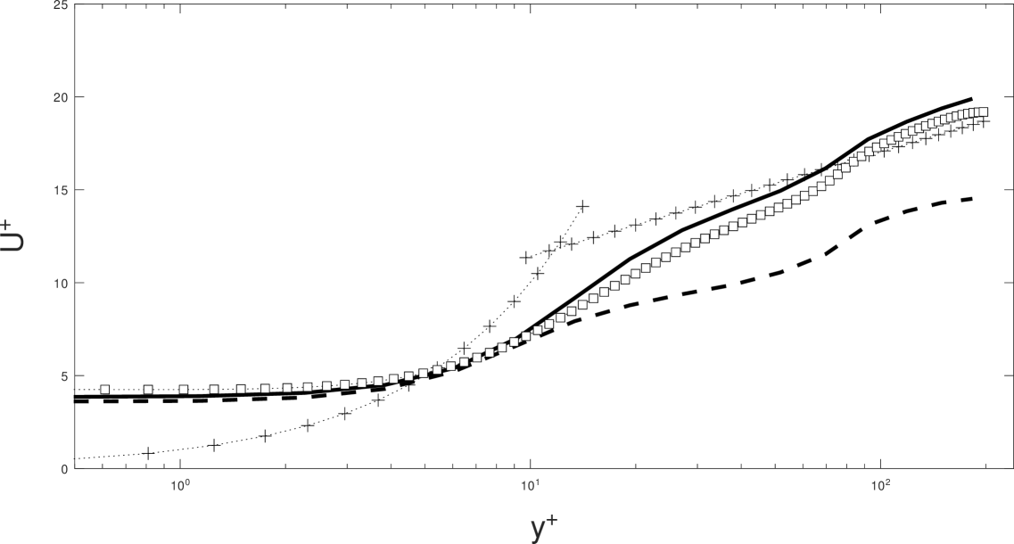
Figure 5: Dimensionless longitudinal velocity $U^{+}$ at the center of the perturbation region for a channel flow with $Re_{\tau}=200$, subjected to a frictionless wall and an adverse pressure gradient step in a narrow region of width $W^{+}=206$. $\Box\cdot\Box\cdot\Box$ , DNS; $---$, $\kappa-\epsilon$ model; solid line, LSTM; $+\cdot+\cdot+$, Law of the Wall, $U^{+}=({1}/{0.41})\ln(y^{+})+5.5$.

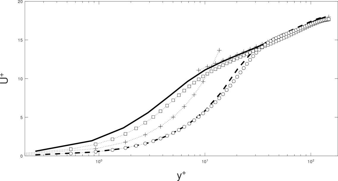
Figure 6: Dimensionless longitudinal velocity $U^{+}$ for a channel flow with $Re_{\tau}=150$, perturbed by wall suction followed by blowing, in a narrow region of total width $W^{+}=412$. Middle of the perturbation: $\Box\cdot\Box\cdot\Box$ , DNS; solid line, LSTM. At a distance of $W^{+}=206$ from the end of the perturbation: $\circ\cdot\circ\cdot\circ\;$, DNS; $---$, LSTM; $+\cdot+\cdot+$, Law of the Wall, $U^{+}=({1}/{0.41})\ln(y^{+})+5.5$.

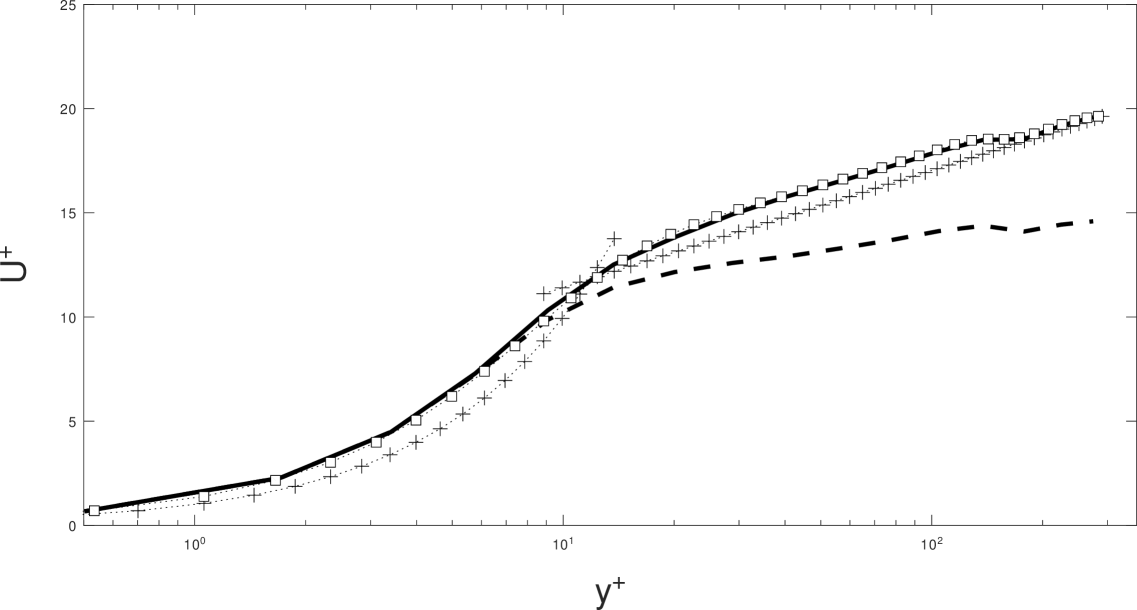
Figure 7: Dimensionless longitudinal velocity $U^{+}$ at a $W^{+}=206$ distance from the end of the perturbation region for a channel flow with $Re_{\tau}\simeq 300$, perturbed by a frictionless wall and a favorable pressure gradient in a narrow region of width $W^{+}=206$. $\Box\cdot\Box\cdot\Box$ , DNS; $---$, $\kappa-\epsilon$ model; solid line, LSTM; $+\cdot+\cdot+$, Law of the Wall, $U^{+}=({1}/{0.41})\ln(y^{+})+5.5$.

This study focuses on moderately low Reynolds number turbulent flows, with the maximum friction Reynolds number $Re_{\tau}$ being 600, which corresponds to $Re_{\delta}\simeq 14,000$. The results serve as a proof of concept, demonstrating the potential for LSTMs to replace traditional RANS turbulence models. However, further research is necessary to extend this approach to higher Reynolds numbers and more complex flow conditions. As mentioned earlier, creating a universal LSTM model that works across a wide range of Reynolds numbers and flow characteristics would likely require a large number of parameters, which could limit its practicality for CFD applications. An alternative approach may involve using specialized neural networks tailored to specific types of turbulent flows. For example, an LSTM model trained exclusively on a DNS database of fully developed turbulent flows over a range of Reynolds numbers could be more efficient for such cases. There would be no need for a more complex LSTM with additional parameters trained on unrelated flow types.

The LSTM predictions are compared with results from the $\kappa-\epsilon$ model and DNS data. The statistics presented include longitudinal velocity ($U$) and shear Reynolds stress (turbulent, viscous, and total) for developed flows, as well as wall skin friction, longitudinal mean velocity, and $\langle uv\rangle$ for perturbed flows, all in dimensionless form.

5.1 Developed Flow

As mentioned earlier, all results presented in this study, using the LSTM neural network, correspond to the 4XBL13BL23BL33DL architecture. Figures 1 and 2 display the mean longitudinal velocity, $U^{+}$, for various Reynolds numbers and the Reynolds shear stress $\langle uv\rangle^{+}$ for developed flow at $Re_{\tau}=200$ and $Re_{\tau}=600$, respectively (both results in dimensionless form using the friction velocity, $u_{\tau}$). These figures highlight the LSTM’s capability to accurately predict the Reynolds shear stress in developed flows, resulting in a correct mean velocity distribution, with good agreement with the ’Law of the Wall’.

The input features for the 4XBL13BL23BL33DL architecture, as listed in Table 2, include $Re_{\tau}$, $S_{11}^{+}$, $S_{12}^{+}$, and $Y$. Here, the plus symbol indicates that these features are nondimensionalized using wall parameters $u_{\tau}$ and $\delta$, except for the wall distance $Y$, which is nondimensionalized by $\delta$ (instead of the usual $y^{+}=yu_{\tau}/\nu$). The inclusion of $Re_{\tau}$ as a feature was motivated by the improvement it provided in predicting $\langle uv\rangle^{+}$ for developed flows. As $Re_{\tau}$ increases, the slope of $\langle uv\rangle^{+}$ in the near-wall region becomes steeper (Fig. 2), making the inclusion of $Re_{\tau}$ essential for accurate predictions under developed flow conditions.

5.2 Skin-Friction for Perturbed Flow

Figures 3 and 4 present the normalized skin-friction coefficient, $f/f_{DF}$ (normalized by the skin-friction coefficient for developed flow, $f_{DF}$), for the RANS simulations based on propagated LSTM predictions, compared with the $\kappa-\epsilon$ model and DNS data. It is important to note that all RANS simulations (both for LSTM propagation and the $\kappa-\epsilon$ model) were performed using the same numerical grid, with identical distances from the wall to the center of the first cell in the grid.

From an applied engineering perspective, the primary objective of a RANS simulation is to accurately compute the mean flow, with particular emphasis on predicting wall skin friction. The shear Reynolds stress, $\langle uv\rangle^{+}$, is crucial in determining the near-wall mean flow distribution, as it influences the wall-normal gradient of the mean velocity. Accurate prediction of $\langle uv\rangle^{+}$ near the wall is therefore essential. In aerodynamic analysis, for example, wall skin friction is a key parameter due to its direct relationship with fuel consumption and other critical factors in vehicle performance evaluation.

Figure 3 shows the abrupt change in $f/f_{DF}$ for a channel flow originally in hydrodynamically developed conditions at $Re_{\tau}=200$, perturbed in a narrow region with width $W^{+}=206$, where a frictionless wall and an adverse pressure gradient step causes the skin friction to drop to zero. This type of perturbation abruptly alters the turbulent momentum fluxes from the channel center toward the wall, strongly affecting the wall skin friction.

Figure 4 presents $f/f_{DF}$ for a developed channel flow at $Re_{\tau}=300$, perturbed by suction from the wall in a narrow region of width $W^{+}=206$, followed by blowing in a similar region. The suction first increases the skin friction as fluid is drawn toward the wall, enhancing the wall-normal mean velocity near the surface. In contrast, the subsequent blowing lifts the fluid away from the wall, causing a sharp decrease in the skin-friction coefficient.

In both figures, the RANS simulations follow the general trend observed in the DNS data, despite the coarse numerical grid used. The performance of the LSTM model surpasses that of the $\kappa-\epsilon$ model, generally providing better alignment with the DNS data outside the perturbation region. To further improve the LSTM’s skin-friction predictions, a denser numerical grid would likely be more effective than merely increasing the number of parameters in the neural network.

5.3 Mean Velocity for Perturbed Flow

Figures 5 to 7 illustrate the distribution of the longitudinal mean velocity, $U^{+}$, for various cases of perturbed channel flow. In Fig. 5, $U^{+}$ is shown at the center of the perturbation region for a flow at $Re_{\tau}=200$, subjected to a frictionless wall and an adverse pressure gradient step. The frictionless wall significantly alters the pure adverse pressure gradient case used for LSTM model training by suspending the turbulent transfer of longitudinal momentum toward the wall. As a result, the mean velocity is modified across the entire channel, and $U^{+}$ no longer follows the ’Law of the Wall’ throughout the domain.

In Fig. 6, the mean velocity predicted by LSTM propagation is compared to DNS data for a channel flow at $Re_{\tau}=150$, perturbed by wall suction followed by blowing within a narrow region of width $W^{+}=412$. This perturbation creates an abrupt increase in the velocity gradient near the wall during suction, followed by a sharp decrease in the gradient during blowing (the wall-normal velocity gradient peaks in the suction region and reaches a minimum in the adjacent blowing region). In this case, the mean flow is substantially modified for $y^{+}<50$, and $U^{+}$ approaches the ’Law of the Wall’ from the midpoint to the channel center. It is evident that $U^{+}$ exceeds the ’Law of the Wall’ mean velocity at the end of the suction region but falls below it at a distance $W^{+}$ from the blowing end. Essentially, suction draws fluid with higher longitudinal momentum toward the wall, increasing the mean velocity in the near-wall region, whereas blowing blocks the mean flow near the wall, reducing the longitudinal mean velocity.

Figure 7 presents $U^{+}$ at a distance $W^{+}$ from the end of the perturbation region for a flow perturbed by a frictionless wall and a favorable pressure gradient step, at $Re_{\tau}=300$. In this case, the mean velocity slightly exceeds the developed condition (surpassing the ’Law of the Wall’) throughout most of the channel, except near the center.

All these figures highlight the strong performance of the LSTM-predicted mean flow, with results closely aligning with DNS data and generally outperforming the $\kappa-\epsilon$ model.

5.4 Shear Reynolds Stress

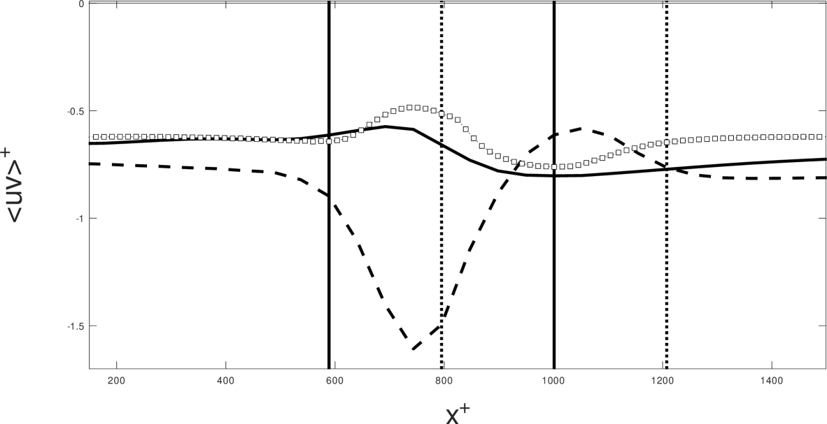
Figure 8: $\langle uv\rangle^{+}$ along $X^{+}$ at $Y^{+}\simeq 17$ from the wall, for a channel flow with $Re_{\tau}\simeq 150$, perturbed with blowing followed by suction in a narrow region of width $W^{+}=412$. $---$$\kappa-\epsilon$; $\Box\cdot\Box\cdot\Box$ , DNS; solid line, LSTM.

As previously mentioned, the RANS simulations based on the LSTM predictions in this study use only the shear Reynolds stress, $\langle uv\rangle^{+}$, while the other Reynolds stresses are set to zero. Figures 8 through 11 compare the LSTM’s predictions of $\langle uv\rangle^{+}$ with DNS data and results from the $\kappa-\epsilon$ model.

The aim of this study is not to critique the $\kappa-\epsilon$ model, which has long been a benchmark for researchers working with RANS simulations. Despite its simplicity, the $\kappa-\epsilon$ model has provided reasonable predictions for a wide range of turbulent flows over the last 50 years. However, it is well-known that the model tends to overestimate turbulence kinetic energy and, consequently, overpredicts $\langle uv\rangle^{+}$. This excessive dissipation leads to an overestimation of the Reynolds shear stress compared to DNS data.

In contrast, while the LSTM predictions do not always align perfectly with DNS data, they consistently exhibit errors due to underestimation. For cases where the absolute value of $\langle uv\rangle^{+}$ exceeds the developed condition, the LSTM model follows this trend but predicts lower absolute values than the DNS results. Similarly, for cases where $\langle uv\rangle^{+}$ is lower than its developed condition, the LSTM predictions again follow this behavior but with reduced absolute values.

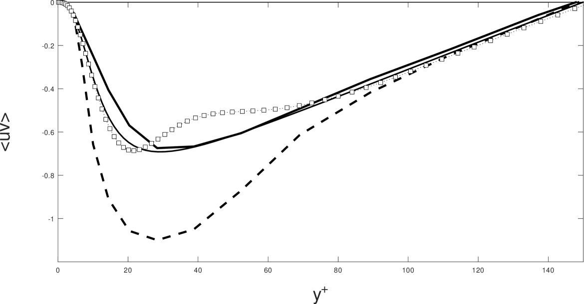
Figure 9: Wall-normal distribution of $\langle uv\rangle^{+}$ at a distance $W^{+}$ from the perturbation end for a flow with $Re_{\tau}\simeq 150$ perturbed by wall suction followed by blowing in a region with a total width of $W^{+}=412$. $---$, $\kappa-\epsilon$ model; $\Box\cdot\Box\cdot\Box$ , DNS; thick solid line, LSTM; thin solid line, DNS in developed condition.

Figure 10: Wall-normal distribution of $\langle uv\rangle^{+}$ at $W+=206$ from the perturbation end for a flow with $Re_{\tau}\simeq 300$ perturbed by a frictionless wall and an adverse pressure gradient step. $---$, $\kappa-\epsilon$ model; $\Box\cdot\Box\cdot\Box$ , DNS; thick solid line, LSTM; thin solid line, DNS in developed condition.

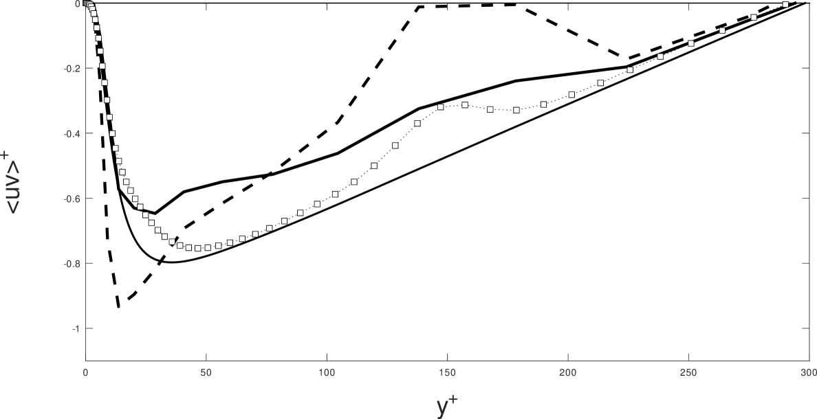
Figure 11: Wall-normal distribution of $\langle uv\rangle^{+}$ at $W+=206$ from the perturbation end for a flow with $Re_{\tau}\simeq 300$ perturbed by a frictionless wall and a favorable pressure gradient step. $---$, $\kappa-\epsilon$ model; $\Box\cdot\Box\cdot\Box$ , DNS; thick solid line, LSTM; thin solid line, DNS in developed condition.

In Fig. 8, the $\langle uv\rangle^{+}$ distribution along the longitudinal direction at $y^{+}\simeq 17$ (where turbulence production is significant) shows that the LSTM model agrees better with DNS data compared to the $\kappa-\epsilon$ model. However, the agreement remains relative, with the LSTM prediction slightly underestimating the DNS data.

A similar trend is observed in Figs. 9 to 11, which depict the wall-normal distributions of $\langle uv\rangle^{+}$ for different cases. In Fig. 9, the DNS data almost matches the developed flow value, and the LSTM model shows minimal deviation from the developed condition, while the $\kappa-\epsilon$ model predicts an excessive value. This conservative behavior of the LSTM model can be viewed as a strength, providing reliable and stable results.

Figures 10 and 11 illustrate cases with perturbations involving a frictionless wall and either an adverse or favorable pressure gradient. These perturbations have opposite effects on the turbulent flow, as reflected in the DNS data. The LSTM predictions follow the same trends but in a more conservative manner, while the $\kappa-\epsilon$ model predicts extreme values of $\langle uv\rangle^{+}$ that significantly exceed DNS results.

Overall, these figures demonstrate the consistent behavior of the LSTM model, which remains conservative compared to the more extreme overpredictions of the $\kappa-\epsilon$ model.

6 Conclusions

This second part of the study (the preprint of the first part is titled ’Modeling Turbulent Flows with LSTM Neural Network’, arXiv:2307.13784v1 [physics.flu-dyn], 25 July 2023) delves deeper into the application of the Long Short-Term Memory (LSTM) artificial recurrent neural network (RNN) as an alternative to traditional Reynolds-Averaged Navier-Stokes (RANS) models. The LSTM model was employed to predict shear Reynolds stress in both developed and developing turbulent channel flows, and these predictions were then propagated in RANS simulations to obtain mean flow solutions. A comparative analysis was performed between LSTM-based results from computational fluid dynamics (CFD) simulations, the outcomes from the $\kappa-\epsilon$ model, and data from direct numerical simulations (DNS). These analyses highlighted the promising performance of the LSTM approach.

The main conclusions of this study, which employed an LSTM architecture with approximately 700 parameters tailored to the characteristics of statistical 2D turbulent channel flows and used as a RANS turbulence model, are as follows.

The LSTM’s propagated predictions were robust, as the turbulent stress values predicted by the model were integrated into computational fluid dynamics (CFD) codes in a stable and reliable manner, at least for the moderately low Reynolds numbers considered in this study. Additionally, the LSTM demonstrated efficacy in non-developed flows, with new RANS simulation cases revealing the model’s effectiveness in capturing turbulence dynamics in perturbed turbulent flows. Despite using a coarse numerical grid in the RANS propagation, the LSTM predictions maintained a reasonable level of accuracy across all cases. Moreover, the LSTM exhibited a conservative behavior, which proved advantageous by providing reliable and stable predictions in comparison to traditional turbulence models.

While this study primarily serves as a proof-of-concept for employing LSTM neural networks in RANS turbulence modeling, this second phase provides strong evidence of its potential as an alternative to conventional models.

Acknowledgments

The author gratefully acknowledge the developers of TensorFlow and Keras for providing these open-source libraries, which were invaluable for the implementation of the machine learning models in this work. The availability of these resources has greatly facilitated the research presented in this preprint.

References

- Pope [2000] S. Pope. Turbulent Flow. University Press, Cambridge, Cambridge, UK, 1st. edition, 2000.
- Pasinato [2023] H. D. Pasinato. Modeling turbulent flows with lstm neural network. arXiv:2307.13784v1[physics.flu-dyn], pages 1–11, 2023.
- Hochriter and Schmidhuber [1997] S. Hochriter and J. Schmidhuber. Long short term memory. Neural Computation, 9:1–32, 1997.
- Sutskever et al. [2014] I. Sutskever, Vinyals O., and Quoc V. Le. Sequence to sequence learning with neural networks. arXiv, pages 1–9, 2014. doi: org/10.48550/arXiv.1409.3215.
- Wu et al. [2019] J. Wu, H. Xiao, R. Sun, and Q. Wang. Reynolds-averaged navier-stokes equations with explicit data-driven reynolds stress closure can be ill-conditioned. J. Fluid Mech., 869:553–596, 2019.
- Thompson et al. [2016] R. L. Thompson, L. B. Sampaio, F. B. Alves, L. Thais, and G. Mompean. A methodology to evaluate statistical errors in dns data of plane channel flows. Comp. Fluids, 130:1–7, 2016.
- Abadi et al. [2015] Martín Abadi, Ashish Agarwal, Paul Barham, Eugene Brevdo, Zhifeng Chen, Craig Citro, Greg S. Corrado, Andy Davis, Jeffrey Dean, Matthieu Devin, Sanjay Ghemawat, Ian Goodfellow, Andrew Harp, Geoffrey Irving, Michael Isard, Yangqing Jia, Rafal Jozefowicz, Lukasz Kaiser, Manjunath Kudlur, Josh Levenberg, Dandelion Mané, Rajat Monga, Sherry Moore, Derek Murray, Chris Olah, Mike Schuster, Jonathon Shlens, Benoit Steiner, Ilya Sutskever, Kunal Talwar, Paul Tucker, Vincent Vanhoucke, Vijay Vasudevan, Fernanda Viégas, Oriol Vinyals, Pete Warden, Martin Wattenberg, Martin Wicke, Yuan Yu, and Xiaoqiang Zheng. TensorFlow: Large-scale machine learning on heterogeneous systems, 2015. URL https://www.tensorflow.org/. Software available from tensorflow.org.
- Brownlee [2017] J. Brownlee. Long Short-term Memory Networks with Python. Machine Learning Mastery, 2017.
- Pasinato [2012] H. D. Pasinato. Dissimilarity of turbulent fluxes of momentum and heat in perturbed turbulent flows. J. Heat Transfer-ASME, 135:1–12, 2012.
- Pasinato [2014] H. D. Pasinato. Direct Numerical Simulation (DNS) of fully developed turbulent channel flow with heat transfer for moderately high Reynolds numbers. Mecánica Computacional, AMCA (http//www.amcaonline.org.ar), XXXIII:287–297, 2014.