Eigenvalues of the Neumann magnetic Laplacian in the unit disk

Abstract

In this paper, we study the first eigenvalue of the magnetic Laplacian with Neumann boundary conditions in the unit disk $\mathbb{D}$ in $\mathbb{R}^{2}$. There is a rather complete asymptotic analysis when the constant magnetic field tends to $+\infty$ and some inequalities seem to hold for any value of this magnetic field leading to rather simple conjectures. Our goal is to explore these questions by revisiting a classical picture of the physicist D. Saint-James theoretically and numerically. On the way, we revisit the asymptotic analysis in light of the asymptotics obtained by Fournais-Helffer that we can improve by combining with a formula stated by Saint-James.

1 Introduction

In this paper, we study the first eigenvalue of the magnetic Laplacian with Neumann boundary conditions in the unit disk $\mathbb{D}$ in $\mathbb{R}^{2}$. Let us formulate the problem more precisely. Using the standard choice

$$\mathbf{A}:x=(x_{1},x_{2})\in\mathbb{R}^{2}\mapsto(-x_{2}/2,x_{1}/2)\in\mathbb{R}^{2}$$

for the so-called magnetic potential, we define the self-adjoint operator $H_{\beta}$ (with $\beta\in\mathbb{R}$) by

$${H_{\beta}u}:=(i\nabla+\beta\,\mathbf{A}(x))^{2}u=-\Delta u+2i\,\beta\,\mathbf{A}\cdot\nabla u+\beta^{2}|\mathbf{A}|^{2}u\,,$$

for all $u$ in the domain

$$\mathcal{D}:=\{u\in H^{2}(\mathbb{D})\,:\,\nabla u\cdot\nu=0\mbox{ on }\partial\mathbb{D}\},$$

where $\nu$ the outward-pointing unit normal. It is well known that $H_{\beta}$ is a self-adjoint operator, non-negative (positive if $\beta\neq 0$), with compact resolvent. Let $\lambda(\beta)$ denote its lowest eigenvalue. Our goal is to understand in detail the dependence of $\lambda(\beta)$ on the parameter $\beta$ (interpreted as the strength of the magnetic field).
The analysis of this Neumann problem is strongly motivated by the analysis of surface superconductivity in physics and the Neumann boundary condition is crucial. At the mathematical level the case of the disk is a way towards understanding the role of the curvature of the boundary. We refer to [2], [19] and to [14] for a presentation of the state of the art in 2014 including works by Baumann-Giorgi-Phillips and Lu-Pan.
Notice that the Dirichlet problem has been analyzed intensively in the last years with similar techniques (see [26, 1] and references therein) but let us emphasize that the phenomena observed in the Neumann case are quite different.

For the analysis of the spectrum $H_{\beta}$, using the radial symmetry of the domain $\mathbb{D}$, we pass to the polar coordinates

$$(x_{1},x_{2})=(r\cos\theta,r\sin\theta)$$

and use a decomposition in Fourier series with respect to the variable $\theta$. We are led to consider the family of $1D$-operators indexed by $n\in\mathbb{Z}$

$$H_{n,\beta}:=-\frac{d^{2}}{dr^{2}}-\frac{1}{r}\frac{d}{dr}+\left(\frac{\beta}{2}r-\frac{n}{r}\right)^{2}\,,$$ (1.1)

with Dirichlet condition at $r=0$ and Neumann condition at $r=1$. The operators $H_{n,\beta}$ are self-adjoint in the Hilbert space $L^{2}((0,1),r\,dr)$.

For each of these operators, we look at the lowest eigenvalue $\lambda(n,\beta)$ as a function of $\beta$. It follows from standard perturbation theory of self-adjoint operators that each map $\beta\mapsto\lambda(n,\beta)$ is real-analytic. We then get the lowest eigenvalue from

$$\lambda(\beta)=\inf_{n\in\mathbb{Z}}\lambda(n,\beta)\,.$$ (1.2)

As explained in Section 2, we can restrict ourselves to $\beta\geq 0$ and $n\in\mathbb{N}$ without loss of generality.

We often find it more convenient to consider auxiliary maps, defined in $(0,+\infty)$ by

$$\beta\mapsto\eta(n,\beta):=\frac{\lambda(n,\beta)}{\beta}$$

and

$$\beta\mapsto\eta(\beta):=\frac{\lambda(\beta)}{\beta}.$$

Our first goal (suggested by previous work and by numerical computations) is to understand the intersection of the curves $\beta\mapsto\lambda(n,\beta)$ and $\beta\mapsto\lambda(n+1,\beta)$ (or, equivalently, of the curves $\beta\mapsto\eta(n,\beta)$ and $\beta\mapsto\eta(n+1,\beta)$). We give a complete proof of a formula due to the physicist D. Saint-James [25].

Theorem 1.1.

Let $n\in\mathbb{N}$ and let us assume that $\beta^{*}$ is a solution in $[0,+\infty)$ of the equation

$$\lambda(n,\beta)=\lambda(n+1,\beta).$$

Then, with the notation

$$\eta^{*}:=\eta(n,\beta^{*})=\eta(n+1,\beta^{*}),$$

we have

$$\beta^{*}=2\eta^{*}+2n+1+\sqrt{(2\eta^{*}+1)^{2}+8n\eta^{*}},$$

and, as a consequence, $\beta^{*}>2(n+1)$.

We then try to understand which $n$ realizes the infimum (1.2) according to the value of $\beta$. We combine the results of M. Dauge and the first author [8, 9], on eigenvalues variation for Sturm-Liouville operators, with Theorem 1.1, to obtain the following result.

Theorem 1.2.

For any $n\in\mathbb{N}$, there exists a unique solution $\beta_{n}$ in $[0,+\infty)$ of the equation

$$\lambda(n,\beta)=\lambda(n+1,\beta).$$

In addition, the sequence $(\beta_{n})_{n\in\mathbb{N}}$ is strictly increasing, and

1. for all $\beta\in[0,\beta_{0}]$, $\lambda(\beta)=\lambda(0,\beta)$;

2. for all $n\in\mathbb{N}\setminus\{0\}$, for all $\beta\in[\beta_{n-1},\beta_{n}]$, $\lambda(\beta)=\lambda(n,\beta)$.

Furthermore, the equation $\lambda(k,\beta)=\lambda(\beta)$, with $\beta\geq 0$, is satisfied only for $k=n$ when $\beta\in(\beta_{n-1},\beta_{n})$, with $n>0$, (only for $k=0$ when $\beta\in[0,\beta_{0}^{*})$) and only for $k\in\{n,n+1\}$ when $\beta=\beta_{n}$ .

Finally, we study the following conjectures.

Conjecture 1.3.

For all $\beta>0$,

$$\eta(\beta)<\Theta_{0}\,.$$

In the above statement, $\Theta_{0}$ is a well-known universal constant, called the De Gennes constant since it was introduced by him [7] in the sixties in the context of Surface Superconductivity (see for mathematical studies [3], and later the book [14] and references therein). This constant is defined

$$\Theta_{0}:=\inf_{\xi\in\mathbb{R}}\lambda^{DG}(\xi)\,,$$ (1.3)

where $\lambda^{DG}(\xi)$ is the lowest eigenvalue of the Neumann realization of the harmonic oscillator

$$\mathfrak{h}_{0}(\xi):=D_{t}^{2}+(t+\xi)^{2}\mbox{ on }\mathbb{R}^{+}\,.$$ (1.4)

Numerically, $\Theta_{0}\simeq 0.590106$ and its first role is to give the asymptotics

$$\lambda(\beta)=\Theta_{0}\beta+o(\beta)$$ (1.5)

as $\beta$ tends to $+\infty$, so that $\eta(\beta)\to\Theta_{0}$.
This property has been known since the nineties and we actually have more accurate asymptotics for the disk, playing an important role in the analysis of more general domains. Our main interest is in the inequality, which is equivalent to $\lambda(\beta)<\Theta_{0}\,\beta$ and in the improvment of the result $\lambda(\beta)<\beta$, proved in [5, Theorem 2.1] for a general domain in $\mathbb{R}^{2}$.

We show in Section 3.5 that Conjecture 1.3 can be deduced from the following other conjecture

Conjecture 1.4.

The sequence $(\eta_{n}^{*})_{n\in\mathbb{N}}$ is strictly increasing, where

$$\eta_{n}^{*}:=\eta(n,\beta_{n})=\eta(n+1,\beta_{n})$$

and $\beta_{n}$ is defined in Theorem 1.2.

We also investigate the so-called strong diamagnetism in $\mathbb{D}$, which states as a conjecture:

Conjecture 1.5.

The map $\beta\mapsto\lambda(\beta)$ is monotonically increasing in the interval $[0,+\infty[$.

It follows from the result of S. Fournais and B. Helffer for a general domain in $\mathbb{R}^{2}$ [13] that the map is ultimately increasing, that is, there exists some $\overline{\beta}>0$ such that $\beta\mapsto\lambda(\beta)$ is increasing in $[\overline{\beta},+\infty[$. The point is to show that, in the case of the disk, the map is increasing in the whole interval $[0,+\infty[$. Let us note that this property is known to hold when the Neumann boundary condition is replaced with Dirichlet (see the PhD thesis of S. Son [26, Theorem 3.3.4]).

In Sections 6 and 4, we present asymptotic and numerical computations supporting these conjectures. We also show how the combination of the results in [13] with the approach followed in the first sections leads to new relations and permits to control the validity of the conjectures in the large magnetic field limit.

Acknowledgements.
This problem has been discussed along the years with many colleagues sharing their ideas. Many thanks to B. Colbois, S. Fournais, A. Kachmar, G. Miranda, M. Persson-Sundqvist, L. Provenzano, and A. Savo for their contributions.

2 Eigenvalue curves

We have, for the operator $H_{n,\beta}$ defined by Equation (1.1),

$$H_{n,\beta}=H_{-n,-\beta},$$

so that, from Equation (1.2), we get

$$\lambda(-\beta)=\lambda(\beta)\,.$$

In addition, a direct computation shows that

$$H_{-n,\beta}=H_{n,\beta}+2n\beta,$$

and therefore, in particular

$$\lambda(-n,\beta)=\lambda(n,\beta)+2n\beta.$$

For $\beta>0$, this implies that the infimum

$$\lambda(\beta)=\inf_{n\in\mathbb{Z}}\lambda(n,\beta)$$

cannot be realized by a negative integer. Thus, if we want to study the map $\beta\mapsto\lambda(\beta)$, it is enough to study the maps $\beta\mapsto\lambda(n,\beta)$ for $n\geq 0$ and $\beta\geq 0$.

For $\beta=0$, we recover the usual Laplacian, with Neumann boundary conditions. We therefore assume in the rest of this section that $\beta>0$. The Sturm-Liouville problem corresponding to $H_{n,\beta}$ is

$$\left\{\begin{array}[]{rl}-f^{\prime\prime}-\frac{1}{r}f^{\prime}+\left(\frac{n}{r}-\frac{\beta}{2}r\right)^{2}f=&\lambda f\mbox{\ \ in \ \ }(0,1)\,,\\ f(0)=0\mbox{ if }n>0,&f^{\prime}(0)=0\mbox{ if }n=0\,,\\ f^{\prime}(1)=&0\,.\end{array}\right.$$ (2.1)

We write $r\mapsto f_{n,\beta}(r)$ for the positive and normalized eigenfunction of (2.1) associated with $\lambda(n,\beta)$.

We can express it using the Kummer function $z\mapsto M(a,b,z)$ (using the conventions and notation of the Digital Library of Mathematical Functions [10, Chapter 13]):

$$f_{n,\beta}(r)=C_{n}^{\beta}r^{n}e^{-\frac{\beta}{4}r^{2}}M\left(\frac{1}{2}-\frac{\lambda}{2\beta},n+1,\frac{\beta}{2}r^{2}\right)$$ (2.2)

where $\lambda=\lambda(n,\beta)$.
Notice (cf [23]) that when $a<c$

$$M(a,c,z)=\frac{\Gamma(c)}{\Gamma(c-a)\Gamma(a)}\int_{0}^{1}e^{zt}t^{a-1}(1-t)^{c-a-1}dt\,.$$ (2.3)

Alternatively, we can use the Whittaker function $z\mapsto M_{\kappa,\mu}(z)$ (see for instance [21, Equation (A.5)]):

$$f_{n,\beta}(r)=\frac{D_{n}^{\beta}}{r}M_{\frac{\lambda}{2\beta}+\frac{n}{2},\frac{n}{2}}\left(\frac{\beta}{2}r^{2}\right).$$ (2.4)

The constants $C_{n}^{\beta}$ and $D_{n}^{\beta}$, depending on $n$ and $\beta$, are chosen so that

$$\int_{0}^{1}f_{n,\beta}(r)^{2}\,r\,dr=1.$$

The eigenvalues of (2.1) (and in particular the first eigenvalue, $\lambda(n,\beta)$) are the roots of the equation

$$(f_{n,\beta})^{\prime}(1)=0$$ (2.5)

(where the left-hand side is understood as the function of $\lambda$ defined by Equation (2.4)). As an illustration, we present in Figure 1 the curves

$$\beta\mapsto\eta(n,\beta)=\frac{\lambda(n,\beta)}{\beta}$$

for $n=0,1,\dots,20\,,$ obtained by solving Equation (2.5) numerically (with computations done in Mathematica).

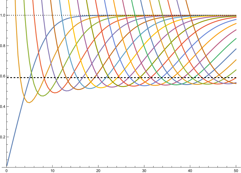
Figure 1: Plot of $\beta\mapsto\eta(n,\beta)=\frac{\lambda(n,\beta)}{\beta}$ for $n$ from 0 to 20. The black dotted line and the black dashed line are the constants $1$ and $\Theta_{0}$ respectively.

In order to study the functions $\beta\mapsto\eta(n,\beta)$, let us give an alternative interpretation of $\eta(n,\beta)$. We perform the change of variable $\rho=\beta^{1/2}r$ and divide by $\beta$. We obtain a new Sturm-Liouville operator $G_{n,\beta}$, which is the Dirichlet-Neumann (Neumann-Neumann if $n=0$) realization in $(0,\beta^{1/2})$ of the differential operator

$$-\frac{d^{2}}{d\rho^{2}}-\frac{1}{\rho}\frac{d}{d\rho}+\Big{(}\frac{n}{\rho}-\frac{\rho}{2}\Big{)}^{2}\,.$$

This new operator is self-adjoint in the Hilbert space $L^{2}((0,\beta^{1/2}),\rho\,d\rho)$ (we recall that the measure has a weight) and $\eta(n,\beta)$ is its first eigenvalue.

3 Properties of the eigenvalue curves

3.1 Asymptotic behavior

Proposition 3.1.

Under the assumption $n>0$, we have, as $\beta\to 0^{+}$,

$$\eta(n,\beta)\sim\frac{(j_{n,1}^{\prime})^{2}}{\beta},$$

where $j_{n,1}^{\prime}$ is the smallest positive zero of $J_{n}^{\prime}$, the derivative of the Bessel function of the first kind $J_{n}$.

In addition, $\eta(0,\beta)\to 0$ as $\beta\to 0^{+}$.

Proof.

By definition, $\eta(n,\beta)=\frac{\lambda(n,\beta)}{\beta}$. From standard perturbation theory, the eigenvalues of $H_{n,\beta}$ converge to the eigenvalues of $H_{n,0}$ as $\beta\to 0$. In particular, $\lambda(n,\beta)\to\lambda(n,0)$. It is easily checked that $\lambda(n,0)=(j_{n,1}^{\prime})^{2}$ (see [20] and references therein).

The last limit follows from the well-known bound $\lambda(0,\beta)\leq\frac{1}{8}\beta^{2}$. This can be obtained by using the constant function $f(r)=1$ in the associated Rayleigh quotient:

$$\lambda(0,\beta)\leq\frac{\int_{0}^{1}1\,({H_{0,\beta}1})\,r\,dr}{\int_{0}^{1}1^{2}\,r\,dr}=\frac{\beta^{2}}{4}\,\frac{\int_{0}^{1}r^{3}\,dr}{\int_{0}^{1}r\,dr}=\frac{\beta^{2}}{8}.\hbox{\hskip 1.0pt\vrule width=4.0pt,height=6.0pt,depth=1.5pt\hskip 1.0pt}\\$$

The following result is a special case of a theorem proved by A. Kachmar and G. Miranda [22, Theorem 1] with techniques inspired by [3].

Proposition 3.2.

As $\beta\to+\infty$,

$$\lambda(n,\beta)=\beta-e^{-\frac{\beta}{2}}\left(\frac{\beta^{n+2}}{2^{n}n!}+o\left(\beta^{n+2}\right)\right).$$

From this proposition we have, as $\beta\to+\infty$,

$$\eta(n,\beta)=1-e^{-\frac{\beta}{2}}\left(\frac{\beta^{n+1}}{2^{n}n!}+o\left(\beta^{n+1}\right)\right).$$ (3.1)

Notice that the Dirichlet case is considered in [1].

3.2 Variations

In Section 2, we have defined the operator $G_{n,\beta}$ and the map $\beta\mapsto\eta(n,\beta)$ for $\beta\in(0,+\infty)$ and $n\in\mathbb{N}$. However, these definitions make sense for any real $n\in[0,+\infty)$. We will use the extended definitions at some points of our analysis. In particular, it follows from standard perturbation theory for self-adjoint operators that the map $(n,\beta)\mapsto\eta(n,\beta)$ is smooth, even real-analytic, and the Feynman-Hellmann formula gives us the derivative of $n\mapsto\eta(n,\beta)$, for a given $\beta>0$:

$$\partial_{n}\eta(n,\beta)=\int_{0}^{\beta^{1/2}}\left(\frac{2n}{\rho^{2}}-1\right)g_{n,\beta}(\rho)^{2}\rho\,d\rho\,,$$ (3.2)

where $g_{n,\beta}$ is the positive and normalized eigenfunction of the operator $G_{n,\beta}$ associated with $\eta(n,\beta)$.

The work of M. Dauge and the first author [8, 9] gives a rather complete picture of the variation of $\beta\mapsto\eta(n,\beta)$ in $(0,+\infty)$, for a given $n\in\mathbb{N}$ (the results actually hold without assuming that $n$ is an integer). The derivatives in the following statements are taken with respect to $\beta$.

Proposition 3.3.

Let $n\in\mathbb{N}$.

1. For all $\beta>0$,

   $${\eta^{\prime}(n,\beta)}=\frac{1}{2}\,\big{(}g_{n,\beta}(\beta^{1/2})\big{)}^{2}\left(\left(\frac{n}{\beta^{1/2}}-\frac{\beta^{1/2}}{2}\right)^{2}-\eta(n,\beta)\right).$$

2. The map $\beta\mapsto\eta(0,\beta)$ is increasing in $[0,+\infty)$.

3. If $n>0$, the map $\beta\mapsto\eta(n,\beta)$ has a unique point of minimum, which is denoted by $\beta_{\min}(n)$. In addition $\beta_{\min}(n)$ is non-degenerate and satisfies

   $$\beta_{\min}(n)>2n\,.$$

To unify the notation, we set

$$\beta_{\min}(0):=0\,.$$ (3.3)

Proof.

Setting $a:=\beta^{1/2}$, $\eta(n,\beta)$ is the first eigenvalue of a Sturm-Liouville operator of the form

$$-\frac{1}{\rho}\,\frac{d}{d\rho}\left(\rho\,\frac{d}{d\rho}\right)+q_{n}(\rho),$$

in the weighted $L^{2}$-space $L^{2}((0,a),\rho\,d\rho)$, with Neumann boundary condition at $\rho=a$ and either Dirichlet (when $n>0$) or Neumann (when $n=0$) boundary condition at $\rho=0$. We write $\mu_{n}(a)=\eta(n,a^{2})$. As in the reference [8], the right endpoint $a$ is variable while the potential

$$q_{n}(\rho)=\left(\frac{n}{\rho}-\frac{\rho}{2}\right)^{2}$$

is independent of $a$.

According to a variant of the Feynman-Hellmann formula [8, Equation ($\rm{F}_{\omega}$) p. 248], for all $a>0$,

$$\mu^{\prime}_{n}(a)=a\,g(a)^{2}\left(q_{n}(a)-\mu_{n}(a)\right),$$

where $g=g_{n,a^{2}}=g_{n,\beta}$. Substituting for $\mu_{n}^{\prime}(\beta^{1/2})$ in

$${\eta^{\prime}(n,\beta)}=\frac{d}{d\beta}\left(\mu_{n}(\beta^{1/2})\right)=\frac{1}{2\beta^{1/2}}\mu_{n}^{\prime}(\beta^{1/2}),$$

we obtain Point (i). Points (ii) and (iii) are direct applications of [8, Theorem 4.2] and [8, Theorem 4.3], respectively.    

As observed in Fournais–Persson-Sundqvist [18], a variant of the first Feynman-Hellmann formula (3.2) gives

$$\lambda^{\prime}(n,\beta)=\int_{0}^{1}\left(\frac{\beta}{2}r^{2}-n\right)f_{n,\beta}(r)^{2}\,r\,dr$$

and therefore:

Lemma 3.4.

If $\beta<2n$, then $\lambda^{\prime}(n,\beta)<0$.

It is also noted in [18] that, using the trial function $f(r)=r^{n}\exp(-\beta r^{2}/4)$ in the Rayleigh quotient, we get:

Lemma 3.5.

If $\beta>2n$, $\lambda(n,\beta)<\beta$ .

3.3 Intersections

Let us prove a useful intermediate result towards the proof of Theorems 1.1 and 1.2.

Proposition 3.6.

Let $n\in\mathbb{N}$. There exists at least one positive $\beta^{*}$ such that $\eta(n,\beta^{*})=\eta(n+1,\beta^{*})$. In addition, any $\beta$ such that $\eta(n,\beta)=\eta(n+1,\beta)$ necessarily satisfies $\beta>2n$.

Proof.

Propositions 3.1 and 3.2 imply, respectively, that $\eta(n,\beta)<\eta(n+1,\beta)$ for $\beta>0$ small enough and $\eta(n,\beta)>\eta(n+1,\beta)$ for $\beta$ large enough. By continuity, there exists at least one $\beta^{*}>0$ such that $\eta(n,\beta^{*})=\eta(n+1,\beta^{*})$.

We prove the second part of the statement by contraposition. Let us use the extended definition of $(m,\beta)\mapsto\eta(m,\beta)$ where $m$ is not necessarily an integer. If $\beta>0$ and $m>0$ are such that $\beta\leq 2m$, Formula (3.2) shows that $\partial_{m}\eta(m,\beta)>0$. In particular, if $0<\beta\leq 2n$, the map $m\mapsto\eta(m,\beta)$ is strictly increasing in $[n,n+1]$, and therefore $\eta(n,\beta)<\eta(n+1,\beta)$.    

It is not clear at this stage that there is no more than one point of intersection between the two curves. We show this in the next two sections.

3.4 Saint-James Formula

Figure 2: Saint-James picture recovered by M. Persson-Sundqvist

The goal of this section is to prove Theorem 1.1. We use a representation for the first eigenfunction of $G_{n,\beta}$ deduced from (2.2) by the relation

$$g_{n,\beta}(\rho)=\beta^{-1/2}f_{n,\beta}(\beta^{-1/2}\rho)\,,$$

that is

$$g_{n,\beta}(\rho)=K_{n}^{\beta}\rho^{n}e^{-\frac{\rho^{2}}{4}}M\left(\frac{1}{2}-\frac{\eta}{2},n+1,\frac{\rho^{2}}{2}\right)$$ (3.4)

(with $\eta=\eta(n,\beta)$ and $K_{n}^{\beta}=\beta^{-1/2}C_{n}^{\beta}$, where $C_{n}^{\beta}$ is the normalization constant in Equation (2.2)).
We obtain

$$(g_{n,\beta})^{\prime}(\rho)=\left(\frac{n}{\rho}-\frac{\rho}{2}\right)g_{n,\beta}(\rho)+K_{n}^{\beta}\,\rho^{n+1}e^{-\frac{\rho^{2}}{4}}\partial_{z}M\left(\frac{1}{2}-\frac{\eta}{2},n+1,\frac{\rho^{2}}{2}\right).$$

Recalling the general formula for the derivative of Kummer functions [10, (13.3.4)]:

$$\partial_{z}M(a,b,z)=\frac{a}{b}M(a+1,b+1,z),$$

we finally get

$$(g_{n,\beta})^{\prime}(\rho)=\left(\frac{n}{\rho}-\frac{\rho}{2}\right)g_{n,\beta}(\rho)+K_{n}^{\beta}\,\frac{\frac{1}{2}-\frac{\eta}{2}}{n+1}\rho^{n+1}e^{-\frac{\beta\rho^{2}}{4}}M\left(\frac{3}{2}-\frac{\eta}{2},n+2,\frac{\rho^{2}}{2}\right)$$

The Neumann condition at $\beta^{1/2}$ (i.e. $(g_{n,\beta})^{\prime}(\beta^{1/2})=0$) leads, after simplifications, to the implicit equation for the eigenvalues $\eta$:

$$(n+1)(n-x)M(\nu,n+1,x)+2x\nu M(\nu+1,n+2,x)=0,$$

with the notation

$$\nu :=\frac{1}{2}(1-\eta),$$

$$x :=\frac{\beta}{2}.$$

Let $(\beta,\eta)$ be a point of intersection of the analytic curves $\beta\mapsto\eta$ for the first eigenvalue of $G_{n,\beta}$ and $G_{n+1,\beta}$. We first note that, according to Proposition 3.6, we have $\beta>2n$. As a consequence, according to Lemma 3.5, $\lambda(n,\beta)<\beta$, so that $0<\eta<1$. The corresponding $(x,\nu)$ satisfies the system of equations

$$(n+1)(n-x)M(\nu,n+1,x)+2x\nu M(\nu+1,n+2,x) =0\,,$$ (3.5)

$$(n+2)(n+1-x)M(\nu,n+2,x)+2x\nu M(\nu+1,n+3,x) =0\,$$ (3.6)

(we have $\nu=\frac{1}{2}(1-\eta)\in(0,\frac{1}{2})$, so the Kummer functions are well-defined).

Remark 3.7.

Since $(g_{n,\beta})^{\prime}(\beta^{1/2})=0$ and since $g_{n,\beta}$ is a non-zero solution of a second-order differential equation, we necessarily have $g_{n,\beta}(\beta^{1/2})\neq 0$, or equivalently $M(\nu,n+1,x)\neq 0$.

We proceed in the following way to obtain an algebraic equation satisfied by $x$ and $\nu$.

• We use the known recursion relations for the functions $M(a,b,z)$ (see for instance [10, Section 13.3]) to express the left-hand side in the system as a linear combination of

  $$X :=M(\nu,n+1,x),$$

  $$Y :=M(\nu,n+2,x).$$

• We write that the determinant of the resulting system is zero (since $(X,Y)\neq(0,0)$, according to Remark 3.7) and we obtain the desired equation.

From the recursion relation [10, (13.3.4)],

$$xM(\nu+1,n+3,x)=(n+2)M(\nu+1,n+2,x)-(n+2)M(\nu,n+2,x)$$ (3.7)

and from [10, (13.3.3)]

$$\nu M(\nu+1,n+2,x)=(n+1)M(\nu,n+1,x)+(\nu-n-1)M(\nu,n+2,x).$$ (3.8)

Inserting Equation (3.8) in Equation (3.5), we get

$$(n+1)(n+x)X+2x(\nu-n-1)Y=0.$$ (3.9)

Inserting Equation (3.7) in Equation (3.6), we get

$$2\nu M(\nu+1,n+2,x)+(n+1-2\nu-x)Y=0.$$

Inserting Equation (3.8) in the previous equation, we obtain

$$2(n+1)X-(n+1+x)Y=0.$$ (3.10)

The system formed by Equations (3.9) and (3.10) is singular if and only if

$$\left|\begin{array}[]{cc}(n+1)(n+x)&2x(\nu-n-1)\\ 2(n+1)&-(n+1+x)\end{array}\right|=0.$$

This gives the equation

$$x^{2}+(4\nu-2n-3)x+n(n+1)=0,$$ (3.11)

which can be rewritten

$$x^{2}-(2\eta+2n+1)x+n(n+1)=0.$$ (3.12)

We revert to the variable $\beta$ and we obtain

$$\beta^{2}-2(2\eta+2n+1)\beta+4n(n+1)=0\,.$$ (3.13)

A similar proof of the same formula is given in [21], using Whittaker functions rather than Kummer functions.

Solving for $\beta$ and using again the necessary condition $\beta>2n$, we finally obtain Saint-James Formula:

$$\beta=2\eta+2n+1+\sqrt{(2\eta+1)^{2}+8\eta n}\,.$$ (3.14)

In addition, since $\eta>0$, Equation (3.14) immediately implies

$$\beta>2(n+1).$$

This completes the proof of Theorem 1.1.

Remark 3.8.

We can rewrite (3.13) in the form

$$(\beta-(2n+1))^{2}=4\lambda+1\,,$$

which holds at the crossing point of $G_{n,\beta}$ and $G_{n+1,\beta}$, with $\eta=\beta\lambda$.
We then get an alternative form of Saint-James formula:

$$\beta=(2n+1)+\sqrt{4\,\lambda+1}\,.$$ (3.15)

3.5 Interlacing between intersections and minima

We study in this section the relation between the points of intersection and the minima $\beta_{\min}(n)$. Our results give in particular a proof of Theorem 1.2. In this section, the derivatives are again taken with respect to $\beta$.

Proposition 3.9.

Let $n\in\mathbb{N}$ and let $\beta^{*}$ be a solution in $(0,\infty)$ of the equation

$$\eta(n,\beta)=\eta(n+1,\beta).$$

Then,

$$\eta^{\prime}(n,\beta^{*})>0$$

and

$$\eta^{\prime}(n+1,\beta^{*})<0.$$

Proof.

We use the notation $\eta^{*}=\eta(n,\beta^{*})=\eta(n+1,\beta^{*})$ and $x^{*}:=\beta^{*}/2$ to make the formulas more readable. A direct computation, using Point (i) of Proposition 3.3, gives

$${\eta^{\prime}(n,\beta^{*})}=c_{n}\frac{(x^{*})^{2}-(2\eta^{*}_{n}+2n+1)x^{*}+n(n+1)}{2x^{*}}$$

and

$${\eta^{\prime}(n+1,\beta^{*})}=c_{n+1}\frac{(x^{*})^{2}-(2\eta^{*}_{n}+2n+3)x^{*}+(n+1)(n+2)}{2x^{*}},$$

with $c_{n}$ and $c_{n+1}$ positive factors. Taking into account that $n$, $x^{*}$ and $\eta^{*}$ satisfy Equation (3.12), we obtain

$${\eta^{\prime}(n,\beta^{*})}=c_{n}\frac{x^{*}-n}{2x^{*}}$$

and

$${\eta^{\prime}(n+1,\beta^{*})}=c_{n+1}\frac{n+1-x^{*}}{2x^{*}}.$$

According to Theorem 1.1, $x^{*}>n+1$, and therefore $\eta^{\prime}(n,\beta^{*})>0$ and $\eta^{\prime}(n+1,\beta^{*})<0$.    

The following theorem is now easy to prove, and implies Theorem 1.2. We use the convention $\beta_{\min}(0)=0$.

Theorem 3.10.

For any $n\in\mathbb{N}$, there exists a unique solution $\beta_{n}$ in $[0,+\infty)$ of the equation

$$\lambda(n,\beta)=\lambda(n+1,\beta).$$

In addition,

1. the sequences $(\beta_{\min}(n))$ and $(\beta_{n})$ are both increasing,

2. for any $n\in\mathbb{N}$, $\beta_{\min}(n)<\beta_{n}<\beta_{\min}(n+1)$,

3. $\lambda(\beta)=\lambda(0,\beta)$ when $\beta\in[0,\beta_{0}]$ and, for $n\in\mathbb{N}\setminus\{0\}$, $\lambda(\beta)=\lambda(n,\beta)$ when $\beta\in[\beta_{n-1},\beta_{n}]$. Furthermore, if $\beta\notin\{\beta_{n}\,:\,n\in\mathbb{N}\}$, there is a unique $k\in\mathbb{N}$ such that $\lambda(\beta)=\lambda(k,\beta)$.

Proof.

Let $\beta^{*}$ be a solution of

$$\eta(n,\beta)=\eta(n+1,\beta).$$

The signs of the derivatives established in Proposition 3.9 imply that

$$\beta_{\min}(n)<\beta^{*}<\beta_{\min}(n+1)$$

(the case $n=0$ is included using the convention that $\beta_{\min}(0)=0$). Let us note that, since at least one solution exists according to Proposition 3.6, we have shown $\beta_{\min}(n)<\beta_{\min}(n+1)$.

By the same argument, any other solution must also belong to the interval

$$(\beta_{\min}(n),\beta_{\min}(n+1)).$$

Since $\beta\mapsto\eta(n,\beta)$ is strictly increasing and $\beta\mapsto\eta(n+1,\beta)$ strictly decreasing in $(\beta_{\min}(n),\beta_{\min}(n+1))$, there cannot be another solution. We now use the notation $\beta_{n}:=\beta^{*}$ and we note that we have proved Point (ii). Since the sequence $(\beta_{\min}(n))$ is increasing, so is the sequence $(\beta_{n})$, which proves Point (i).

To prove Point (iii), we remark that multiplying the values $\eta(n,\beta)$ by $\beta$ does not change their ordering, so that $\lambda(n,\beta)<\lambda(n+1,\beta)$ for $\beta<\beta_{n}$ and $\lambda(n,\beta)>\lambda(n+1,\beta)$ for $\beta>\beta_{n}$. Combining this with the fact that the sequence $(\beta_{n})$ is increasing, we first deduce that, for $\beta\in(0,\beta_{0})$,

$$\lambda(0,\beta)<\lambda(1,\beta)<\lambda(2,\beta)<\dots\,,$$

and in particular $\lambda(\beta)=\lambda(\beta,0)$. Then, for any $n\in\mathbb{N}\setminus\{0\}$ and $\beta\in(\beta_{n-1},\beta_{n})$, we find

$$\lambda(n,\beta)<\lambda(n+1,\beta)<\lambda(n+2,\beta)<\dots$$

and

$$\lambda(0,\beta)>\lambda(1,\beta)>\dots>\lambda(n-1,\beta)>\lambda(n,\beta).$$

In particular, $\lambda(\beta)=\lambda(n,\beta)$. This establishes Point (iii) when $\beta$ is not a point of intersection. The full statement follows by continuity.    

Combining Point (iii) of the previous theorem with the inequality $\beta_{\min}(n)>2n$ (Point (iii) of Proposition 3.3) and with Lemma 3.5, we obtain

$$\lambda(\beta)<\beta\,.$$

This inequality is proved for a general domain in $\mathbb{R}^{2}$ by Colbois-Léna-Provenzano-Savo [6].

Let us now recall the definition

$$\eta_{n}^{*}:=\eta(n,\beta_{n})=\eta(n+1,\beta_{n})$$

appearing in the statement of Conjecture 1.5.

Since $\eta(\beta)=\eta(n+1,\beta)$ for $\beta\in[\beta_{n},\beta_{n+1}]$ and since $\beta\mapsto\eta(n+1,\beta)$ is decreasing in $[\beta_{n},\beta_{\min}(n+1)]$ and increasing in $[\beta_{\min}(n+1),\beta_{n+1}]$, we have

$$\eta(n+1,\beta)\leq\max\{\eta_{n}^{*},\eta_{n+1}^{*}\}\mbox{ for all }\beta\in[\beta_{n},\beta_{n+1}]\,.$$ (3.16)

In addition,

$$\eta(\beta)\leq\eta_{0}^{*}\mbox{ for all }\beta\in(0,\beta^{*}_{0}]\,,$$ (3.17)

since $\eta(\beta)=\eta(0,\beta)$ and $\beta\mapsto\eta(0,\beta)$ is strictly increasing in $(0,\beta_{0}^{*}]$.

Conjecture 1.3 is therefore equivalent to

$$\eta^{*}_{n}<\Theta_{0}\mbox{ for all }n\in\mathbb{N}.$$ (3.18)

From known asymptotic results (1.5), $\eta_{n}^{*}$ tends to $\Theta_{0}$. Therefore, it would be enough to prove that the sequence $(\eta^{*}_{n})$ is strictly increasing to obtain Inequality (3.18). This shows that Conjecture 1.4 implies Conjecture 1.3.

Notice also that we can deduce from (3.13) that if Conjecture 1.5 holds, i. e. if $\lambda(\beta)$ is increasing then

$$\beta_{n+1}\geq 2+\beta_{n}\,.$$ (3.19)

In particular it holds for $n$ large enough, using Fournais-Helffer [12] monotonicity result, which will be recalled in Section 4 and analyzed in more detail. This will also be confirmed numerically for $n\leq 20$.

4 Asymptotic results for the disk revisited

Starting from the asymptotic analysis given in [13] we show that these asymptotics could be refined at the intersection points i.e. for the sequence $\beta_{n}$ as $n\rightarrow+\infty$. We then show how the comparison with the information coming from Saint-James formula leads to complete asymptotics of $\beta_{n}$ and $\lambda(\beta_{n})=\lambda(n,\beta_{n})$. This validates asymptotically a conjecture on the monotonicity of $\beta_{n+1}-\beta_{n}$.

4.1 The case of the disk (reminder after [12])

With (1.3) in mind, we also recall that $\xi_{0}<0$ is the point where $\xi\mapsto\lambda^{DG}(\xi)$ attains its unique (non degenerate) minimum and that $C_{1}$ is given by

$$C_{1}=\frac{u_{0}^{2}(0)}{3}\;.$$ (4.1)

where $u_{0}=\phi_{\xi_{0}}$, is the positive, normalized eigenfunction associated with $\lambda^{DG}(\xi_{0})$.
Numerically (see [4], [12] or [24])

$$C_{1}\sim 0.254\,,\,\xi_{0}\sim-0.768\,.$$

We also recall that

$$\Theta_{0}=\xi_{0}^{2}\,.$$ (4.2)

Theorem 4.1 (Eigenvalue asymptotics for the disk).

Suppose that $\mathbb{D}$ is the unit disk. Define $\delta(m,\beta)$, for $m\in{\mathbb{Z}}$, $\beta>0$, by

$$\delta(m,\beta)=m-\tfrac{\beta}{2}-\xi_{0}\sqrt{\beta}.$$ (4.3)

Then there exist (computable) constants $C_{0},\delta_{0}\in{\mathbb{R}}$ such that if

$$\Delta_{\beta}=\inf_{m\in{\mathbb{Z}}}|\delta(m,\beta)-\delta_{0}|\;,$$ (4.4)

then

$$\lambda(\beta)=\Theta_{0}\beta-C_{1}\sqrt{\beta}+3C_{1}\sqrt{\Theta_{0}}\big{(}\Delta_{\beta}^{2}+C_{0}\big{)}+{\mathcal{O}}(\beta^{-\frac{1}{2}})\;.$$ (4.5)

The asymptotics (4.5) is deduced (see the proof in [13] or a more detailed analysis in the next subsection) from the asymptotics

$$\lambda(m,\beta)=\Theta_{0}\beta-C_{1}\sqrt{\beta}+3C_{1}\sqrt{\Theta_{0}}\big{(}|\delta(m,\beta)-\delta_{0}|^{2}+C_{0}\big{)}+{\mathcal{O}}(\beta^{-\frac{1}{2}})\,,$$ (4.6)

and then considering the infimum.
Although not used here, notice that the $3D$-case was analyzed by Helffer-Morame and in the verssion with three terms in [16].

4.2 Theorem 4.1 revisited

We now revisit the proof of Theorem 4.1 as given in [13] (see also [16]) in order to improve its conclusions when considering $\beta=\beta_{n}$.

We start with the Neumann operator

$$\mathfrak{h}_{0}(\zeta)=-\frac{d^{2}}{d\tau^{2}}+(\tau+\zeta)^{2}$$

on $L^{2}({\mathbb{R}}_{+},d\tau)\;.$

Let $D(t)=\{x\in{\mathbb{R}}^{2}\,|\,|x|\leq t\}$ be the disc with radius $t$. Let $\widetilde{Q}_{\beta}$ be the quadratic form

$$\widetilde{Q}_{\beta}[u]=\int_{D(1)\setminus D(\frac{1}{2})}\big{|}(-i\nabla-\beta{\bf A})u\big{|}^{2}\,dx\;,$$

with domain $\{u\in H^{1}(D(1)\setminus D(\frac{1}{2}))\,|\,u(x)=0\text{ on }|x|=\frac{1}{2}\}$. Let $\tilde{\lambda}(\beta)$ be the lowest eigenvalue of the corresponding self-adjoint operator (Friedrichs extension). Using the Agmon estimates in the normal direction, it can be proved

$$\lambda(\beta)=\tilde{\lambda}(\beta)+{\mathcal{O}}(\beta^{-\infty})\;.$$ (4.7)

By changing to boundary coordinates (if $(r,\theta)$ are usual polar coordinates, then $t=1-r$, $s=\theta$), the quadratic form $\widetilde{Q}_{\beta}[u]$ becomes,

$$\widetilde{Q}_{\beta}[u] =\int_{0}^{2\pi}ds\int_{0}^{1/2}dt\,(1-t)^{-1}|(D_{s}-\beta\tilde{A}_{1})u|^{2}+(1-t)|D_{t}u|^{2}\;,$$ (4.8)

$$\|u\|_{L^{2}}^{2} =\int_{0}^{2\pi}ds\int_{0}^{1/2}dt\,(1-t)|u|^{2}\;,\quad\tilde{A}_{1}=\tfrac{1}{2}-t+\tfrac{t^{2}}{2}\;.$$

Performing the scaling $\tau=\sqrt{\beta}\,t$ and decomposing in Fourier modes,

$$u=\sum_{m}e^{ims}\phi_{m}(t)\;,$$

leads to

$$\tilde{\lambda}(\beta)=\beta\inf_{m\in{\mathbb{Z}}}e_{\delta(m,\beta),\beta}\;.$$ (4.9)

Here the function $\delta(m,\beta)$ was defined in (4.3) and $e_{\delta,\beta}$ is the lowest eigenvalue of the operator $\mathfrak{h}(\delta,\beta)$ associated with the quadratic form $q_{\delta,\beta}$ on $L^{2}((0,\sqrt{\beta}/2);(1-\beta^{-1/2}\tau))d\tau)$ (with Neumann boundary condition at $0$ and Dirichlet at $\sqrt{\beta}/2$):

$$q_{\delta,\beta}[\phi]=\int_{0}^{\sqrt{\beta}/2} (1-\tfrac{\tau}{\sqrt{\beta}})^{-1}\big{(}(\tau+\xi_{0})+\beta^{-\frac{1}{2}}(\delta-\tfrac{\tau^{2}}{2})\big{)}^{2}$$

$$+(1-\tfrac{\tau}{\sqrt{\beta}})|\phi^{\prime}(\tau)|^{2}\,d\tau\;.$$ (4.10)

The self-adjoint Neumann operator ${\mathfrak{h}}(\delta,\beta)$ associated with $q_{\delta,\beta}$ (on the space $L^{2}((0,\sqrt{\beta}/2);(1-\beta^{-1/2}\tau)d\tau)$) is

$${\mathfrak{h}}(\delta,\beta) =-(1-\tfrac{\tau}{\sqrt{\beta}})^{-1}\frac{d}{d\tau}(1-\tfrac{\tau}{\sqrt{\beta}})\frac{d}{d\tau}$$

$$\quad+(1-\tfrac{\tau}{\sqrt{\beta}})^{-2}\big{(}(\tau+\xi_{0})+\beta^{-\frac{1}{2}}(\delta-\tfrac{\tau^{2}}{2})\big{)}^{2}\;.$$ (4.11)

We will only consider $\delta$ varying in a fixed bounded set. In this case, we know that there exists a $d>0$ such that if $\beta>d^{-1}$, then the spectrum of $\mathfrak{h}(\delta,\beta)$ contained in $(-\infty,\Theta_{0}+d)$ consists of exactly one simple eigenvalue.

We can formally develop ${\mathfrak{h}}(\delta,\beta)$ as

$${\mathfrak{h}}(\delta,\beta)={\mathfrak{h}}_{0}+\beta^{-\frac{1}{2}}{\mathfrak{h}}_{1}+\beta^{-1}{\mathfrak{h}}_{2}+{\mathcal{O}}(\beta^{-\frac{3}{2}})\;.$$

with

$${\mathfrak{h}}_{0} =-\frac{d^{2}}{d\tau^{2}}+(\tau+\xi_{0})^{2}\;,$$

$${\mathfrak{h}}_{1} =\frac{d}{d\tau}+2(\tau+\xi_{0})(\delta-\tfrac{\tau^{2}}{2})+2\tau(\tau+\xi_{0})\;,$$

$${\mathfrak{h}}_{2} =\tau\frac{d}{d\tau}+(\delta-\tfrac{\tau^{2}}{2})^{2}+4\tau(\tau+\xi_{0})(\delta-\tfrac{\tau^{2}}{2})+3\tau^{2}(\tau+\xi_{0})^{2}\;.$$ (4.12)

Let $u_{0}$ be the ground state eigenfunction of ${\mathfrak{h}}_{0}$ with eigenvalue $\Theta_{0}$, where ${\mathfrak{h}}_{0}$ is considered as a selfadjoint operator on $L^{2}({\mathbb{R}}_{+};d\tau)$ with Neumann boundary condition at $0$. Let $R_{0}$ be the regularized resolvent, which is defined by

$$R_{0}\phi=\begin{cases}({\mathfrak{h}}_{0}-\Theta_{0})^{-1}\phi\;,&\phi\perp u_{0}\;,\\ \quad 0\;,&\phi\parallel u_{0}\,.\end{cases}$$

Here the orthogonality is measured with respect to the usual inner product in $L^{2}({\mathbb{R}}_{+};d\tau)$.

Let $\lambda_{1}$ and $\lambda_{2}$ be given by

$$\lambda_{1} :=\langle u_{0}\,|\,{\mathfrak{h}}_{1}u_{0}\rangle\;, \lambda_{2} :=\lambda_{2,1}+\lambda_{2,2}\;,$$

$$\lambda_{2,1} :=\langle u_{0}\,|\,{\mathfrak{h}}_{2}u_{0}\rangle\;, \lambda_{2,2} :=\langle u_{0}\,|\,({\mathfrak{h}}_{1}-\lambda_{1})u_{1}\rangle\;,$$ (4.13)

Here the inner products are the usual inner products in $L^{2}({\mathbb{R}}_{+};d\tau)$. The functions $u_{1},u_{2}$ are given as

$$u_{1} =-R_{0}({\mathfrak{h}}_{1}-\lambda_{1})u_{0}\;, u_{2} =-R_{0}\big{\{}({\mathfrak{h}}_{1}-\lambda_{1})u_{1}+({\mathfrak{h}}_{2}-\lambda_{2})u_{0}\big{\}}\;.$$ (4.14)

Notice that $u_{0}\in{\mathcal{S}}(\overline{{\mathbb{R}}_{+}})$ and that $R_{0}$ maps ${\mathcal{S}}(\overline{{\mathbb{R}}_{+}})$ (continuously) into itself. Therefore, $u_{0},u_{1},u_{2}$ (and their derivatives) are rapidly decreasing functions on ${\mathbb{R}}_{+}$.

Let $\chi\in C_{0}^{\infty}({\mathbb{R}})$ be a usual cut-off function, such that

$$\chi(t) =1\quad\text{ for }|t|\leq\tfrac{1}{8}\;, {\rm supp}\chi \subset[-\tfrac{1}{4},\tfrac{1}{4}]\;,$$ (4.15)

and let $\chi_{\beta}(\tau)=\chi(\tau\beta^{-\frac{1}{4}})$ .

Our trial state is defined by

$$\psi:=\chi_{\beta}\big{\{}u_{0}+\beta^{-\frac{1}{2}}u_{1}+\beta^{-1}u_{2}\big{\}}\;.$$ (4.16)

A calculation (using in particular the exponential decay of the involved functions) gives that

$$\big{\|}\big{\{}{\mathfrak{h}}(\delta,\beta)-\big{(}\Theta_{0}+\lambda_{1}\beta^{-\frac{1}{2}}+\lambda_{2}\beta^{-1}\big{)}\big{\}}\psi\big{\|}_{L^{2}([0,\sqrt{\beta}/2];(1-\beta^{-1/2}\tau)d\tau)}={\mathcal{O}}(\beta^{-\frac{3}{2}})\;,$$

$$\|\psi\|_{L^{2}([0,\sqrt{\beta}/2];(1-\beta^{-1/2}\tau)d\tau)}=1+{\mathcal{O}}(\beta^{-\frac{1}{2}})\;,$$ (4.17)

where the constant in ${\mathcal{O}}$ is uniform for $\delta$ in bounded sets.

Therefore, we have proved that (uniformly for $\delta$ varying in bounded sets)

$$e_{\delta,B}=\Theta_{0}+\lambda_{1}\beta^{-\frac{1}{2}}+\lambda_{2}\beta^{-1}+{\mathcal{O}}(\beta^{-\frac{3}{2}})\;.$$ (4.18)

It remains to calculate $\lambda_{1},\lambda_{2}$ and, in particular, deduce their dependence on $\delta$.

A standard calculation (which can for instance be found in [13, Section 2]) gives that

$$\lambda_{1}=-C_{1}\;.$$ (4.19)

It was harder to calculate $\lambda_{2}$ explicitly but it is proven in [13] that

$$\lambda_{2}(\delta)=3C_{1}\sqrt{\Theta_{0}}\big{(}(\delta-\delta_{0})^{2}+C_{0}\big{)}\;.$$ (4.20)

Remembering (4.7) and (4.9) this finishes the proof of Theorem 4.1. A computation of $\delta_{0}$ will be given later.

The same proof (but pushing the expansion further as done for instance in [16]) gives the following extension

Proposition 4.2.

For any $2\leq N\in\mathbb{N}$, uniformly for $\delta$ varying in bounded sets, we have

$$e_{\delta,\beta}=\Theta_{0}+\lambda_{1}\beta^{-\frac{1}{2}}+\lambda_{2}(\delta)\beta^{-1}+\sum_{j=3}^{N}\lambda_{j}(\delta)\beta^{-j/2}+{\mathcal{O}}(\beta^{-\frac{N+1}{2}})\;.$$ (4.21)

Moreover the $\lambda_{j}(\delta)$ are polynomials of $\delta$.

Proof.

Following the previous proof (corresponding to $N=2$)

$$\psi_{N}:=\chi_{\beta}\big{\{}\sum_{j=0}^{N}\beta^{-\frac{j}{2}}u_{j}\}$$ (4.22)

and

$$\big{\|}\big{\{}{\mathfrak{h}}(\delta,\beta)-\big{(}\Theta_{0}+\lambda_{1}\beta^{-\frac{1}{2}}+\sum_{j=2}^{N}\lambda_{j}(\delta)\beta^{-j/2}\big{)}\big{\}}\psi_{N}\big{\|}_{L^{2}([0,\sqrt{\beta}/2];(1-\beta^{-1/2}\tau)d\tau)}={\mathcal{O}}(\beta^{-\frac{N+1}{2}})\;,$$

$$\|\psi_{N}\|_{L^{2}([0,\sqrt{\beta}/2];(1-\beta^{-1/2}\tau)d\tau)}=1+{\mathcal{O}}(\beta^{-\frac{1}{2}})\;,$$ (4.23)

where the constant in ${\mathcal{O}}$ is uniform for $\delta$ in bounded sets.
Note for later that the normalized eigenfunction $u_{\delta,\beta}$ associated with $e_{\delta,\beta}$ satisfies, for any interval $(0,M)$ and any $N$,

$$||u_{\delta,\beta}-u_{0}-\sum_{j=1}^{N}\beta^{-\frac{j}{2}}\hat{u}_{j}||_{H^{1}(0,M;1-\beta^{-1/2}\tau)d\tau)}\leq C_{M,N}\beta^{-(N+1)/2}\,,$$ (4.24)

for $\beta$ large enough.
Here the $\hat{u}_{j}$ are in $\mathcal{S}(\overline{\mathbb{R}_{+}})$ and depend polynomially of $\delta$.   

Combining with (4.7), (4.9) and considering for $n$ large $\beta=\beta_{n}$, we obtain

Corollary 4.3.

For any $N$, we have with $\beta=\beta_{n}$ and $\delta=\delta(n,\beta_{n})$

$$\lambda_{1}(\beta_{n})=\lambda(n,\beta_{n})=\beta\Big{(}\Theta_{0}+\lambda_{1}\beta^{-\frac{1}{2}}+\lambda_{2}(\delta)\beta^{-1}+\sum_{j=3}^{N}\lambda_{j}(\delta)\beta^{-j/2}+{\mathcal{O}}(\beta^{-\frac{N+1}{2}})\Big{)}\,.$$ (4.25)

Theorem 4.4.

There exist sequences $\hat{\delta}_{j}$ ($j\geq 1$) and $\hat{\lambda}_{j}$ ($j\geq 3$) such that, for any $N$, we have

$$\delta(n,\beta_{n})=\delta_{0}-\frac{1}{2}+\sum_{1\leq j\leq N}\hat{\delta}_{j}\,\beta_{n}^{-j/2}+{\mathcal{O}}(\beta_{n}^{-\frac{N+1}{2}})\,,$$ (4.26)

and

$$\lambda_{1}(\beta_{n})/\beta_{n}=\Theta_{0}+\lambda_{1}\,\beta_{n}^{-\frac{1}{2}}+\lambda_{2}(\delta_{0}-\frac{1}{2})\,\beta_{n}^{-1}+\sum_{j=3}^{N}\check{\lambda}_{j}\,\beta_{n}^{-j/2}+{\mathcal{O}}(\beta_{n}^{-\frac{N+1}{2}})\,.$$ (4.27)

To get (4.26), we simply compare the expansions given for $\lambda_{1}(n,\beta_{n})$ (i.e $\delta=\delta(n,\beta_{n})$ and $\lambda_{1}(n+1,\beta_{n})$ (i.e. $\delta=\delta(n+1,\beta_{n})$).

Let us describe the first step in more detail. We use (4.5) for $\beta=\beta_{n}$:

$$\lambda(\beta_{n})/\beta_{n}=\Theta_{0}-C_{1}(\beta_{n})^{-1/2}+3C_{1}\Theta_{0}^{1/2}\big{(}(\delta(n,\beta_{n})-\delta_{0})^{2}+C_{0}\big{)}(\beta_{n})^{-1}+\mathcal{O}(\beta_{n}^{-3/2})\,.$$ (4.28)

At the crossing we get, by using (4.6) for $\beta=\beta_{n}$ and for both $m=n$ and $m=n+1$,

$$\delta(n,\beta_{n})+\delta(n+1,\beta_{n})=2\delta_{0}+\mathcal{O}(\beta_{n}^{-1/2})\,.$$ (4.29)

which implies using (4.3), (4.26) and

$$\delta_{0}-\delta(n,\beta_{n})=\frac{1}{2}+\mathcal{O}(\beta_{n}^{-1/2})\,.$$ (4.30)

Hence we obtain at the crossing point $\beta_{n}$

$$\frac{\lambda(\beta_{n})}{\beta_{n}}:=\eta_{n}^{*}=\Theta_{0}-C_{1}(\beta_{n})^{-1/2}+3C_{1}\Theta_{0}^{1/2}(\frac{1}{4}+C_{0})(\beta_{n})^{-1}+\mathcal{O}(\beta_{n}^{-3/2})\,.$$ (4.31)

All these formulas correspond to an asymptotic as $n\rightarrow+\infty$.
By recursion we get expansions at any order.

Remark 4.5.

Combining with (3.15) at $\beta_{n}$ we get, using (4.26) and (4.27),

$$\delta_{0}=\frac{1}{2}\Theta_{0}^{-1/2}C_{1}\sim 0.0975\,.$$ (4.32)

This formula seems to be new and was not obtained in [13].

Notice that we have not at the moment mixed these results with the Saint-James formula.    

4.3 Implementation of Saint-James formula

In this subsection, we give a complete expansion for $\beta_{n}$ as a series in powers of $n^{-1/2}$.

Theorem 4.6.

There is an infinite sequence $\hat{\kappa}_{j}$ ($j\geq 0$) such that

$$\beta_{n}=2n+\xi_{1}n^{\frac{1}{2}}+\hat{\kappa}_{0}+\sum_{j\geq 1}\hat{\kappa}_{j}n^{-j/2}+\mathcal{O}(n^{-\infty})\,,$$ (4.33a)

with

$$\xi_{1}=-2^{3/2}\xi_{0}\,,\,\hat{\kappa}_{0}=1-2\delta_{0}+2\xi_{0}^{2}\,.$$ (4.33b)

In particular, this implies

Corollary 4.7.

$$\gamma_{n}:=\beta_{n+1}-\beta_{n}=2+\frac{\xi_{1}}{2}n^{-1/2}+\hat{\gamma}_{2}n^{-1}+\hat{\gamma}_{3}n^{-3/2}+\mathcal{O}(n^{-2})\,.$$ (4.34)

and

$$\gamma_{n}-\gamma_{n+1}=-\frac{1}{4}\xi_{1}n^{-3/2}+\mathcal{O}(n^{-2})\,.$$ (4.35)

This in particular proves for $n$ large that the sequence $\gamma_{n}$ is decreasing.

Proof of Theorem 4.6
To prove (4.33), we implement our candidate for the expansion into (3.15) which reads at $\beta_{n}$:

$$\beta_{n}-(2n+1)=\sqrt{4\lambda(n,\beta_{n})+1}\,.$$

The $\hat{\kappa}_{j}$ are then obtained by recursion.

Let us more explicitly describe the first step.
We start from (3.15) at $\beta=\beta_{n}$ but we implement (4.27)

$$\lambda(\beta_{n})=\beta_{n}\big{(}\Theta_{0}-C_{1}(\beta_{n})^{-1/2}+3C_{1}\Theta_{0}^{1/2}(\frac{1}{4}+C_{0})(\beta_{n})^{-1}\big{)}+\mathcal{O}(n^{-1/2})\,.$$ (4.36)

This leads to

$$4\lambda(\beta_{n})+1=4\beta_{n}\big{(}\Theta_{0}-C_{1}(\beta_{n})^{-1/2}+C_{2}(\beta_{n})^{-1}\big{)}+\mathcal{O}(n^{-1/2})\,,$$

with

$$C_{2}:=3C_{1}\Theta_{0}^{1/2}(\frac{1}{4}+C_{0})+\frac{1}{4}\,.$$

We then get

$$\sqrt{4\lambda(\beta_{n})+1}=2\Theta_{0}^{\frac{1}{2}}\beta_{n}^{1/2}\big{(}1-C_{1}\Theta_{0}^{-1}\beta_{n}^{-1/2}+C_{2}\Theta_{0}^{-1}\beta_{n}^{-1}+\mathcal{O}(n^{-3/2})\big{)}^{\frac{1}{2}}$$

which implies

$$\sqrt{4\lambda(\beta_{n})+1}=2\Theta_{0}^{\frac{1}{2}}\beta_{n}^{1/2}-C_{1}\Theta_{0}^{-1/2}+C_{3}\Theta_{0}^{-1}\beta_{n}^{-1/2}+\mathcal{O}(n^{-1})\,,$$

with $C_{3}$ computable.
This leads to

$$\beta_{n}=2n+1+2\Theta_{0}^{\frac{1}{2}}\beta_{n}^{1/2}-C_{1}\Theta_{0}^{-1/2}+C_{3}\Theta_{0}^{-1}\beta_{n}^{-1/2}+\mathcal{O}(n^{-1})\,.$$

Implementing $\beta_{n}=2n+\xi_{1}n^{\frac{1}{2}}+\hat{\kappa}_{0}+\hat{\kappa}_{1}n^{-1/2}+\mathcal{O}(n^{-1})$, we get the existence of explicit $\hat{\kappa}_{0}$ (as given in the statement) and $\hat{\kappa}_{1}$.    

5 Strong diamagnetism revisited

5.1 Reminder and first approach

In the case of the disk, it was also proved in [12] the following statement called “strong diamagnetism”.

Theorem 5.1.

Let $\mathbb{D}$ be the disk. Then the left- and right-hand derivatives $\lambda_{\pm}^{\prime}(\beta)$ exist and satisfy

$$\lambda_{+}^{\prime}(\beta)\leq\lambda_{-}^{\prime}(\beta)\;,$$

$$\liminf_{\beta\rightarrow+\infty}\lambda_{+}^{\prime}(\beta)\geq\Theta_{0}-\tfrac{3}{2}C_{1}|\xi_{0}|>0\;.$$ (5.1)

In particular, $\beta\mapsto\lambda(\beta)$ is strictly increasing for large $\beta$.

Notice that the strong magnetism in dimension 3 is considered by Soeren Fournais and Mikael Persson Sundqvist in [16]. Our analysis of the Saint-James picture has given a more precise description by determining the sequence $(\beta_{n})$ where the left and right derivatives could differ. It is now interesting to combine the informations given by the two approachs.

But let us come back to $\lambda(n,\beta)$ since we are interested in the asymptotics of $\lambda^{\prime}(n,\beta)$. Hence we start from

$$\lambda(n,\beta)=\Theta_{0}\beta+\lambda_{1}\beta^{\frac{1}{2}}+\lambda_{2}(\delta(n,\beta)))+\sum_{j=3}^{N}\lambda_{j}(\delta(n,\beta))\beta^{1-j/2}+{\mathcal{O}}(\beta^{1-\frac{N+1}{2}})\,,$$

which is a consequence of (4.7), (4.9) and (4.21).
We rewrite this as

$$\lambda(n,\beta)=g_{N}(\beta)+r_{N}(\beta)\,,$$

with

$$g_{N}(\beta):=\Theta_{0}\beta+\lambda_{1}\beta^{\frac{1}{2}}+\lambda_{2}(\delta(n,\beta)))+\sum_{j=3}^{N}\lambda_{j}(\delta(n,\beta))\beta^{1-j/2}\,.$$

The problem is that it could be difficult to prove directly that we can differentiate the expansion, since we have no good control of $r^{\prime}_{N}(\beta)$.
One way to avoid this difficulty is to use the observation in [12] that, for any $\epsilon>0$,

$$\lambda_{+}^{\prime}(\beta) =-2\Re\langle\phi_{{+}}(\beta)\,|\,{\bf A}\cdot(-i\nabla-\beta{\bf A})\phi_{{+}}(\beta)\rangle$$

$$=\frac{1}{\epsilon}\langle\phi_{{+}}(\beta)\,|\,\big{(}H_{\beta+\epsilon}-H_{\beta}-\epsilon^{2}{\bf A}^{2}\big{)}\phi_{{+}}(\beta)\rangle\;,$$

where $\phi_{+}(\gamma)$ is a suitable eigenfunction depending analytically of $\gamma$ around $\beta$ and associated with $\lambda(\gamma)$ for $\gamma\in[\beta,\beta+\epsilon)$. Therefore, the variational principle implies

$$\lambda_{+}^{\prime}(\beta)\geq\frac{\lambda(\beta+\epsilon)-\lambda(\beta)}{\epsilon}-\epsilon\|{\bf A}\|_{L^{\infty}(\Omega)}^{2}\,,$$

and we have trivially

$$\lambda_{+}^{\prime}(\beta)\leq\frac{\lambda(\beta+\epsilon)-\lambda(\beta)}{\epsilon}\,.$$

For $\epsilon>0$ small enough, it is consequently sufficient to have an expansion of $\frac{\lambda(\beta+\epsilon)-\lambda(\beta)}{\epsilon}$.
For $\beta=\beta_{n}$, we have

$$\frac{\lambda(\beta_{n}+\epsilon)-\lambda(\beta_{n})}{\epsilon}=\epsilon^{-1}\Big{(}g_{N}(\beta_{n}+\epsilon))-g_{N}(\beta_{n})\Big{)}+\epsilon^{-1}{\mathcal{O}}((\beta_{n})^{1-\frac{N+1}{2}})$$

But we can control $g_{N}(\beta)$ and its derivatives (note that $\delta^{\prime}(m,\beta)=\mathcal{O}(1)$, $\delta^{\prime\prime}=\mathcal{O}(\beta^{-3/2})$,…..)
Using its Taylor expansion, with remainder term and taking $N$ large and $\epsilon=(\beta_{n})^{-N/2}$, we can justify the differentiation term by term of the expansion of $\lambda(n,\beta)$. In particular we get:

$$\lambda_{+}^{\prime}(\beta_{n})=\Theta_{0}+\frac{3}{2}C_{1}|\xi_{0}|+\check{C}_{2}(\beta_{n})^{-1/2}+\mathcal{O}((\beta_{n})^{-1})\,.$$ (5.2)

End of the proof.

We only give the details for the first step. We recall that

$$\delta_{0}-\delta(n,\beta_{n})=\frac{1}{2}+\delta_{1}n^{-1/2}+\mathcal{O}(n^{-1})\,.$$ (5.3)

Now we can differentiate (4.6). So we get

$$\lambda^{\prime}(m,\beta)=\Theta_{0}-C_{1}\beta^{-1/2}+6C_{1}\sqrt{\Theta_{0}}\big{(}\delta(m,\beta)-\delta_{0})\delta^{\prime}(m,\beta)\big{)}+\mathcal{O}(\beta^{-1/2})\,,$$ (5.4)

Observing that

$$\delta^{\prime}(m,\beta)=-\frac{1}{2}-\frac{1}{2}\xi_{0}\beta^{-1/2}$$

we get

$$\lambda^{\prime}(m,\beta)=\Theta_{0}-C_{1}\beta^{-1/2}-3C_{1}\sqrt{\Theta_{0}}(\delta(m,\beta)-\delta_{0})(1+\xi_{0}\beta^{-1/2})+\mathcal{O}(\beta^{-1/2})\,,$$ (5.5)

We apply this formula with $m=n$, $\beta=\beta_{n}$,

$$\lambda^{\prime}(n,\beta_{n})=\Theta_{0}-C_{1}\beta^{-1/2}+3C_{1}\sqrt{\Theta_{0}}(\frac{1}{2}+\delta_{1}n^{-1/2}+\mathcal{O}(n^{-1}))(1+\xi_{0}\beta^{-1/2})+\mathcal{O}(\beta^{-1/2})\,,$$ (5.6)

$$\lambda^{\prime}(n,\beta_{n})=\Theta_{0}+\frac{3}{2}C_{1}\sqrt{\Theta_{0}}+\hat{C}_{1}n^{-1/2}+\mathcal{O}(n^{-1})\,.$$ (5.7)

Hence we have a two terms expansion which improves (5.16).
Using the more complete expansion, we get

Theorem 5.2.

We have

$$\lambda^{\prime}(n,\beta_{n})=\Theta_{0}+\frac{3}{2}C_{1}\sqrt{\Theta_{0}}+\sum_{j\geq 1}\hat{C}_{1}n^{-j/2}+\mathcal{O}(n^{-\infty})\,.$$ (5.8)

We will give an alternative proof in Subsection 5.4.

5.2 About $f_{n,\beta_{n}}$.

We would like to consider the proof of

$$\lim_{n\rightarrow+\infty}(\beta_{n})^{-1/2}|f_{n,\beta_{n}}(1)|^{2}=3C_{1}=u_{0}(0)^{2}\,,$$

and prove more generally

$$(\beta_{n})^{-1/2}|f_{n,\beta_{n}}(1)|^{2}=u(0)^{2}+\sum_{j\geq 1}\check{C}_{j}n^{-j/2}+\mathcal{O}(n^{-\infty})\,.$$ (5.9)

This is actually a consequence of the comparison between $f_{n,\beta}$ and the quasi-mode constructed in (4.24). Taking the trace at $0$, we get

$$u_{\delta(n,\beta),\beta}(0)=u_{0}(0)+\sum_{j=1}^{N}\hat{c}_{j}(\delta)\beta^{-1/2}+\mathcal{O}(\beta^{-(N+1)/2})\,.$$

We finally observe that

$$f_{n,\beta}(1)=\beta^{1/4}u_{\delta(n,\beta),\beta}(0)+\mathcal{O}(\beta^{-\infty})\,.$$

The power of $\beta$ appears when doing the change of variable $t=\beta^{-1/2}\tau$. The error comes from the comparison between the disk and the annulus. We can take $\beta=\beta_{n}$ and the comparison between $\beta_{n}$ and $n$ to obtain a $2$-term asymptotics.
Using the complete expansion of $\delta_{n}(n,\beta_{n})$ we have

Proposition 5.3.

For any $N>0$,

$$\beta_{n}^{-1/4}f_{n,\beta_{n}}(1)=u_{0}(0)+\sum_{j\geq 1}^{N}\check{\kappa}_{j}\beta_{n}^{-j/2}+\mathcal{O}(\beta^{-(N+1)/2})\,.$$ (5.10)

or

$$\beta_{n}^{-1/4}f_{n,\beta_{n}}(1)=u_{0}(0)+\sum_{j\geq 1}^{N}\kappa_{j}n^{-j/2}+\mathcal{O}(n^{-(N+1)/2})\,.$$ (5.11)

This in particular proves (5.9).

5.3 Feynman-Hellmann formula in the asymptotic limit

In order to support Conjecture 1.5, let us present some additional results on the variation of $\beta\mapsto\lambda(n,\beta)$. Some of these computations appear already in [18].

Proposition 5.4.

For $n\in\mathbb{N}$, for all $\beta>0$,

$$\lambda^{\prime}(n,\beta)=\frac{\lambda(n,\beta)}{\beta}-\frac{1}{2\beta}\left(\lambda(n,\beta)-\big{(}n-\frac{\beta}{2}\big{)}^{2}\right)|f_{n,\beta}(1)|^{2}\,.$$ (5.12)

Proof.

Using the notation of Sections 2 and 3, we have, for $\beta>0$,

$$\lambda(n,\beta)=\beta\,\eta(n,\beta)$$

and

$$\lambda^{\prime}(n,\beta)=\eta(n,\beta)+\beta\,\eta^{\prime}(n,\beta)\,.$$

Using Point (i) of Proposition 3.3, we get

$$\lambda^{\prime}(n,\beta)=\eta(n,\beta)+\frac{\beta}{2}|g_{n,\beta}(\beta^{1/2})|^{2}\left(\left(\frac{n}{\beta^{1/2}}-\frac{\beta^{1/2}}{2}\right)^{2}-\eta(n,\beta)\right).$$

Since $g_{n,\beta}(\beta^{1/2})=\beta^{-1/2}f_{n,\beta}(1)$, we obtain the desired formula.    

5.4 Application to the strong diamagnetism

We can use Formula (5.12) to evaluate numerically the right derivative of $\beta\mapsto\lambda(\beta)$ at the points of intersection $\beta_{n}$. Indeed, it follows from Theorem 1.2 that

$$\lambda^{\prime}_{+}(\beta_{n})=\lambda^{\prime}(n+1,\beta_{n})\,,$$ (5.13)

and

$$\lambda^{\prime}_{-}(\beta_{n})=\lambda^{\prime}(n,\beta_{n})\,,$$ (5.14)

Assuming that Conjecture 1.5 is true, we should find $\lambda^{\prime}_{+}(\beta_{n})\geq 0$.

On the asymptotic side, using the proof in [12] leading to Theorem 5.1, we get

$$\lim_{n\rightarrow+\infty}\lambda^{\prime}(n+1,\beta_{n})=\Theta_{0}-\frac{3}{2}C_{1}|\xi_{0}|\,,$$ (5.15)

and

$$\lim_{n\rightarrow+\infty}\lambda^{\prime}(n,\beta_{n})=\Theta_{0}+\frac{3}{2}C_{1}|\xi_{0}|\,.$$ (5.16)

Numerically,

$$\Theta_{0}-\frac{3}{2}C_{1}|\xi_{0}| \sim 0.297350,$$

$$\Theta_{0}+\frac{3}{2}C_{1}|\xi_{0}| \sim 0.882863.$$

Let us compute the term which appears in (5.12),

$$\frac{1}{2\beta_{n}}\left(\lambda(n,\beta_{n})-\big{(}n-\frac{\beta_{n}}{2}\big{)}^{2}\right)\,.$$

We have, using the improvement of (4.26),

$$n-\frac{\beta_{n}}{2}=\xi_{0}(\beta_{n})^{1/2}+\delta_{0}-\frac{1}{2}+\mathcal{O}(n^{-1/2})\,,$$

and the expansion of $\lambda(n,\beta_{n})$ given in (4.27), we obtain

$$\lambda(n,\beta_{n})-\big{(}n-\frac{\beta_{n}}{2}\big{)}^{2}=(-C_{1}-2\xi_{0}(\delta_{0}-\frac{1}{2}))(\beta_{n})^{\frac{1}{2}}+\mathcal{O}(1)\,,$$

and

$$(\beta_{n})^{-1}\Big{(}\lambda(n,\beta_{n})-\big{(}n-\frac{\beta_{n}}{2}\big{)}^{2}\Big{)}=\xi_{0}(\beta_{n})^{-\frac{1}{2}}+\mathcal{O}(n^{-1})\,.$$

Using the asymptotics of $\beta_{n}$, $\lambda(\beta_{n})$ and a complete expansion for $f_{n,\beta_{n}}$, we have a second proof of Theorem 5.2. Using (5.14) and (5.13) we obtain

Theorem 5.5.

We have

$$\lambda^{\prime}_{+}(\beta_{n})=\Theta_{0}+\frac{3}{2}C_{1}\sqrt{\Theta_{0}}+\sum_{j\geq 1}\hat{C}_{j}n^{-j/2}+\mathcal{O}(n^{-\infty})\,.$$ (5.17)

and

$$\lambda^{\prime}_{-}(\beta_{n})=\Theta_{0}-\frac{3}{2}C_{1}\sqrt{\Theta_{0}}+\sum_{j\geq 1}\tilde{C}_{j}n^{-j/2}+\mathcal{O}(n^{-\infty})\,.$$ (5.18)

6 Numerical study of the points of intersection

Using the formulas of Subsection 3.4 we look for an equation for $\nu$ as a function of $n$. We recall that for a pair $(x,\nu)$ corresponding to an intersection between $\beta\mapsto\eta(n,\beta)$ and $\beta\mapsto\eta(n+1,\beta)$, we have (3.14), that is

$$x=(1-2\nu+n+\frac{1}{2})+\frac{1}{2}\sqrt{(3-4\nu)^{2}+8(1-2\nu)n}\,,$$

and (3.5), that is

$$(n+1)(n-x)M(\nu,n+1,x)+2x\nu M(\nu+1,n+2,x)=0\,.$$

By elimination of $x$, we get the equation

$$\Phi(\nu,n)=0\,$$ (6.1)

a priori satisfied for $(\nu_{n},n)$ with $n\in\mathbb{N}$ but which could be analyzed for $n\in\mathbb{R}^{+}$.

Using Mathematica, we determined numerically the points of intersection $(\beta_{n},\hat{\eta}_{n})$ of the curves $\beta\mapsto\eta(n,\beta)$ and $\beta\mapsto\eta(n+1,\beta)$ by solving for $(\beta,\eta)$ in the non-linear system consisting of Equations (3.5) and (3.6), with the integer $n$ ranging from $0$ to $400$. These points are displayed on Figure 3 as black dots, for $n$ from 0 to $19$. A sample of the results for larger $n$ is presented in Table 1. This computation does not use the Saint-James Formula (3.14). The superscript is used to distinguish these numerical values from those obtain by a second method. We note that the sequence $(\hat{\eta}_{n})$ appears to be increasing.

Table 1: Solutions of the non-linear system

$n$	$\beta_{n}^{(1)}$	$\eta_{n}^{(1)}$
0	3.847538710016439	0.46188467750410933
1	6.784689992385673	0.490953836999826
2	9.495696565685895	0.5057893193465876
3	12.091164794355297	0.5152514126454681
4	14.613601105384173	0.5219883372745205
5	17.08457097842645	0.5271130898896494
10	28.989490930878333	0.5418512305407657
25	62.88412636538398	0.55750340973811
50	117.3339755112376	0.5663294771262841
100	223.66235051600012	0.5729419029706077
200	432.6371167436942	0.5777978340023635
300	639.5318373766472	0.5799955549150178
400	845.3470994716895	0.5813189732301576

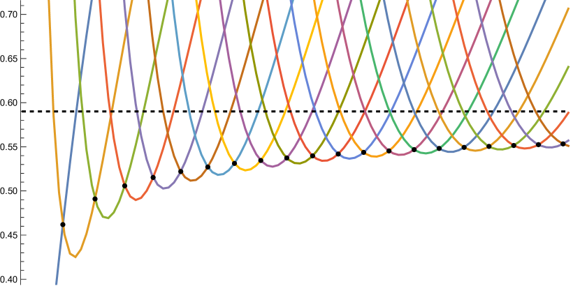
Figure 3: Zoom on the plot of $\beta\mapsto\eta(n,\beta)$ for $n$ de 0 a 20. The black dashed line is the constant $\Theta_{0}$. The black dots mark the points $(\beta_{n}^{(1)},\hat{\eta}_{n}^{(1)})$.

Let us recall that the sequence $\gamma_{n}:=\beta_{n+1}-\beta_{n}$ converges to $2$ and, more precisely, admits an asymptotic expansion of the form

$$\gamma_{n}=2+\sum_{j\geq 1}c_{j}\,n^{-j/2}+O\left(n^{-\infty}\right).$$

After applying four times Richardson extrapolation, we obtain a sequence $(R_{4}\gamma_{n})$ satisfying

$$R_{4}\gamma_{n}=2+\mathcal{O}\left(n^{-5/2}\right)$$

The new sequence therefore has the same limit as the original, with a much faster convergence, and can be used to check numerically the value of the limit. The results are presented in Table 2.

Table 2: Sequence $\gamma_{n}=\beta_{n+1}-\beta_{n}$

$n$	$\gamma_{n}$	$R_{4}\gamma_{n}$
0	2.9371512823692343
1	2.7110065733002218	1.992309139244719
2	2.595468228669402	1.999385754276766
3	2.5224363110288763	2.0000780253629706
4	2.470969873042275	2.0001506529324526
5	2.4322005977636465	2.000134587773707
6	2.4016457058734133	2.000108698821863
7	2.376764086900799	2.0000863469016394
8	2.355993937178809	2.000068928763249
9	2.338315624735216	2.000055641011863
10	2.3230315388610627	2.00004548367877
24	2.2159762440866757	2.0000068128960815
50	2.1516833824983337
100	2.107942427892027
200	2.076571962353569
300	2.0625877291374763
399	2.0542993010602686

We computed the sequence $(\eta_{n}^{(2)})$, for the same values of $n$, by a second method: numerically solving Equation (6.1), which is itself deduced from the Saint-James Formula 3.14. The results are presented in Table 3, with the relative variation from the results of the first method, defined as

$$\varepsilon_{n}:=\frac{|\eta_{n}^{(2)}-\eta_{n}^{(1)}|}{\eta_{n}^{(1)}}.$$

The close agreement confirms the Saint-James Formula and suggests that our numerical computations are rather accurate.

Table 3: Solutions of the implicit equation, with the relative variation from Table 1

$n$	$\eta_{n}^{(2)}$	$\varepsilon_{n}$
0	3.8475387100164355	$10^{-15}$
1	6.784689992385671	$2\times 10^{-15}$
2	9.495696565685904	$10^{-15}$
3	12.091164794355297	$3\times 10^{-15}$
4	14.613601105384173	$3\times 10^{-15}$
5	17.084570978426473	$2\times 10^{-15}$
10	28.989490930878333	$9\times 10^{-16}$
25	62.884126365384006	$2\times 10^{-15}$
50	117.3339755112376	$2\times 10^{-16}$
100	223.66235051600046	$10^{-15}$
200	432.63711674369415	$10^{-15}$
300	639.5318373766468	$10^{-15}$
400	845.3470994716891	$10^{-15}$

Finally, we present the numerical results concerning the left and right derivatives of $\lambda(\beta)$ at $\beta=\beta_{n}$, obtained with Mathematica, in Table 4.

To compare the limits (5.15) and (5.16) with our numerics, we proceed as we did for the sequence $(\gamma_{n})$, applying four times Richardson extrapolation to the numerical sequences. The results are displayed in Table 4.

All these numerical checks appear consistent with the asymptotic results of Sections 4 and 5.

Table 4: Left and right derivatives at the points of intersection

$n$	$\beta_{n}$	$\lambda^{\prime}(n,\beta_{n})$	$\lambda^{\prime}(n+1,\beta_{n})$	$R_{4}\lambda^{\prime}(n,\beta_{n})$	$R_{4}\lambda^{\prime}(n+1,\beta_{n})$
0	3.84754	0.884743	0.144907
1	6.78469	0.880478	0.178114	0.883010	0.298037
2	9.49570	0.879482	0.195254	0.882910	0.297498
3	12.0912	0.879172	0.206280	0.882882	0.297401
4	14.6136	0.879085	0.214181	0.882872	0.297374
5	17.0846	0.879088	0.220223	0.882868	0.297363
6	19.5168	0.879130	0.225048	0.882866	0.297357
7	21.9184	0.879190	0.229024	0.882861	0.297355
8	24.2952	0.879257	0.232376	0.882864	0.297353
9	26.6512	0.879326	0.235256	0.882864	0.297352
10	28.9895	0.879394	0.237767	0.882863	0.297352
25	62.8841	0.880145	0.256706	0.882863	0.297350
50	117.334	0.880738	0.267540
100	223.662	0.881254	0.275737
200	432.637	0.881671	0.281801
300	639.532	0.881870	0.284558
400	845.347	0.881993	0.286222

References

• [1] M. Baur and T. Weidl. Eigenvalues of the magnetic dirichlet lapla- cian with constant magnetic field on discs in the strong field limit. arXiv:2402.01474 (2024).
• [2] A. Bernoff and P. Sternberg. Onset of superconductivity in decreasing fields for general domains. J. Math. Phys. 39 (1998), 1272–1284.
• [3] C. Bolley, B. Helffer. An application of semi-classical analysis to the asymptotic study of the supercooling field of a superconducting material. Annales de l’I.H.P. Physique théorique (1993). Vol.: 58 (2), 189-233.
• [4] V. Bonnaillie. Analyse mathématique de la supraconductivité dans un domaine à coins : méthodes semi-classiques et numériques. Thèse de Doctorat, Université Paris 11 (2003).
• [5] B. Colbois, C. Léna, L. Provenzano, and A. Savo. Geometric bounds for the magnetic Neumann eigenvalues in the plane. Journal de Mathématiques Pures et Appliquées 179, 454-497 (2023).
• [6] B. Colbois, C. Léna, L. Provenzano, and A. Savo. A reverse Faber-Krahn inequality for the magnetic Laplacian. Journal de Mathématiques Pures et Appliquées 192, 103632 (2024).
• [7] P.G. de Gennes. Boundary effects in superconductors. Rev. Mod. Phys. January 1964.
• [8] M. Dauge, B. Helffer. Eigenvalues Variation. I. Neumann Problem for Sturm-Liouville Operators. Journal of Differential Equations 104 (2), 243-262, (1993).
• [9] M. Dauge, B. Helffer. Eigenvalues Variation. II. Multidimensional Problems. Journal of Differential Equations 104 (2), 263-297 (1993).
• [10] NIST Digital Library of Mathematical Functions. https://dlmf.nist.gov/, Release 1.2.0 of 2024-03-15. F. W. J. Olver, A. B. Olde Daalhuis, D. W. Lozier, B. I. Schneider, R. F. Boisvert, C. W. Clark, B. R. Miller, B. V. Saunders, H. S. Cohl, and M. A. McClain, eds.
• [11] S. Fournais and B. Helffer. Accurate eigenvalue asymptotics for the magnetic Neumann Laplacian. Ann. Inst. Fourier 56(1), p. 1-67 (2006).
• [12] S. Fournais and B. Helffer. On the third critical field in Ginzburg-Landau theory. Comm. Math. Phys. 266 (2006), no. 1, 153–196.
• [13] S. Fournais and B. Helffer. Strong diamagnetism for general domains and applications. Annales de l’Institut Fourier, Tome 57 (2007) no. 7, 2389-2400.
• [14] S. Fournais and B. Helffer. Spectral Methods in Surface Superconductivity. Progress in Nonlinear Differential Equations and Their Applications, Vol. 77, Birkhäuser (2010).
• [15] S. Fournais and B. Helffer. Inequalities for the lowest magnetic Neumann eigenvalue. Letters in Mathematical Physics, Volume 109, pages 1683–1700, (2019).
• [16] S. Fournais and M. Persson. Strong diamagnetism for the ball in three dimensions. Asymptotic analysis, Vol. 72, Issue 1, 77-123. (2009).
• [17] S. Fournais and M. Persson Sundqvist. Lack of Diamagnetism and the Little–Parks Effect. Commun. Math. Phys. 337, 191–224 (2015).
• [18] S. Fournais and M. Persson Sundqvist. Calculations for the disc. Unpublished (2017).
• [19] B. Helffer and A. Morame. Magnetic bottles in connection with superconductivity. J. Funct. Anal. 185 (2), 604-680 (2001).
• [20] B. Helffer and M. Persson Sundqvist. On nodal domains in Euclidean balls. Proc. Amer. Math. Soc. 144 (2016), no. 11, 4777–4791.
• [21] A. Kachmar, V. Lotoreichik, and M. Persson-Sundqvist. On the Laplace operator with a weak magnetic field in exterior domains. ArXiv:2405.18154v1 (2024).
• [22] A. Kachmar and G. Miranda. The magnetic Laplacian on the disc for strong magnetic fields. Arxiv: 2407.11241v1 (2024).
• [23] W. Magnus, F. Oberhettinger and R.P. Soni. Formulas and theorems for the special functions of mathematical physics, 3rd enlarged ed, Grundlehren der Mathematischen Wissenschaften, Volume 52, Springer, (1966).
• [24] M. Persson Sundqvist. Magnetic model operators. A short review and something new. Lecture at conference in honor of the 70th birthday of Bernard Helffer. April 2019.
• [25] D. Saint-James. Etude du champ critique $HC3$ dans une géométrie cylindrique. Physics Letters, (15)(1) 13-15 (1965).
• [26] S. Soojin Son. Spectral Problems on Triangles and Discs: Extremizers and Ground States. PhD thesis. 2014.
url: https://www.ideals.illinois.edu/items/49400.