FLMarket: Enabling Privacy-preserved Pre-training Data Pricing for Federated Learning

Abstract.

Federated Learning (FL), as a mainstream privacy-preserving machine learning paradigm, offers promising solutions for privacy-critical domains such as healthcare and finance. Although extensive efforts have been dedicated from both academia and industry to improve the vanilla FL, little work focuses on the data pricing mechanism. In contrast to the straightforward in/post-training pricing techniques, we study a more difficult problem of pre-training pricing without direct information from the learning process. We propose FLMarket that integrates a two-stage, auction-based pricing mechanism with a security protocol to address the utility-privacy conflict. Through comprehensive experiments, we show that the client selection according to FLMarket can achieve more than 10% higher accuracy in subsequent FL training compared to state-of-the-art methods. In addition, it outperforms the in-training baseline with more than 2% accuracy increase and 3$\times$ run-time speedup.

1. Introduction

Federated Learning (FL) provides a privacy-preserving paradigm without exposing private data for learning machine learning (ML) models (Deng et al., 2021b; Liu et al., 2020; Nagalapatti and Narayanam, 2021). It has found an increasing number of applications such as medical information systems (Dayan et al., 2021), financial data analysis (Basu et al., 2021), and cross-border corporate data integration (Wan et al., 2023). Research and industry efforts on FL primarily focus on improving the accuracy (Li et al., 2020; Wang et al., 2020), computation (Lai et al., 2021; Nishio and Yonetani, 2019) and communication performance (Perazzone et al., 2022; Ribero and Vikalo, 2020), as well as enhancing security and privacy (Wang et al., 2022; Bonawitz et al., 2017). However, little attention has been paid to incentivizing the participants to join FL, which is crucial because valuable data is not readily available for FL tasks without proper incentives.

Pre-Training Pricing for FL Data Market. In traditional centralized ML tasks, servers (such as companies) typically purchase the training data they need from a data market. These data are often collected, cleaned, and pre-processed at considerable cost by third parties (Schomm et al., 2013; Liu and Hacigümüs, 2014). A typical FL data market has three entities: data sellers (clients) who generate data and participate in FL tasks (Spiekermann et al., 2015), model buyers who purchase the model and FL data market (server) that coordinates between sellers and buyers (Zheng et al., 2022).

Existing incentive mechanisms mainly target the in/post-training pricing based on the accuracy improvement of FL training (Zhan et al., 2020; Tang and Wong, 2021; Zhan et al., 2021). Unfortunately, the data providers (FL clients) cannot anticipate the reward before contributing their data and resources. Meanwhile, data buyers cannot evaluate the data quality before the actual training takes place. These are crucial because (1) anticipated rewards before training can greatly encourage the participation of clients, increasing client enrollment and the diversity of training data (Zeng et al., 2022; Zhan et al., 2021). (2) Clients who know the early-estimated pricing before training are more likely to continue, which guarantees the stability of FL training (Lai et al., 2021). For instance, based on our empirical survey , 84.7% of respondents believe that pre-training incentives increase their willingness to participate in FL. Additionally, 82.7% of respondents prefer FL training with pre-training rewards over post-training rewards. Therefore, a framework for pre-training evaluation and pricing is indispensable for a sustainable FL data market.

Use Case. A medical research institution aims to develop a model for disease diagnosis and there are several healthcare providers with patient data. The medical research institution first publishes the task in the FL data market with the total payments. Then the task is forwarded to the corresponding healthcare providers to ask for their willingness to join. All healthcare providers who intend to participate in the training task negotiate a satisfactory reward for contributing their data. Hence, the data market collaborates with them to negotiate and establish reasonable pricing as an anticipated reward for subsequent FL training. To this end, the FL marketplace must have the ability to determine the price of each participating client before performing the actual FL training.

Challenges. Compared to the conventional in/post-training pricing (Liu et al., 2020; Wang et al., 2019; Song et al., 2019; Zeng et al., 2022; Zhan et al., 2021), implementing pre-training pricing is inherently challenging:

Challenge 1: Pre-training pricing require to value clients’ data without direct model feedback. The first challenge comes from limited information before training, i.e., we cannot use aggregated model accuracy as direct feedback for pricing and client selection. Instead, we need to peek into the statistics such as volume and categorical distributions, and analyze their correlations with model accuracy in a federated setting (Deng et al., 2021b).

Challenge 2: Pre-training pricing requires a consensus agreement between client and server. An optimal pricing system should effectively balance the needs of both the client and the server. From the client’s perspective, pricing should not only reflect the intrinsic value of their data but also offer incentives that encourage them to share their data. On the server side, the total compensation should remain within budgetary limits, and the price set for each client should meet or exceed their expected value.

Challenge 3: Pre-training pricing requires to solve the privacy-utility conflict. Although data volume and class distribution bring more insights for pre-training pricing, they also ask the clients to share distributional information regarding their private data. E.g., knowing the distribution of human activities would easily reveal individual habits (Qian et al., 2020; Deshpande and Karypis, 2004), hence deviating from the original intention of FL to preserve privacy.

Our Solution. To tackle the above challenges, we present FLMarket, an fairness, incentive, privacy-preserving client pricing framework for the FL data market. The price is determined through an auction that consists of a two-stage pricing mechanism, i.e., the initial price based on the statistical information and a contribution-proportional allocation strategy. The first-phase pricing determine the price of each client based on its statistical information and computed by a data value score function. To avoid client’s sensitive information leakage, we design a privacy-preserving protocol to enable secured sharing of private distributions with the server. In addition, the second-phase pricing determine the actual payment of the selected clients through Budget-constrained Pricing Mechanism which is a consensus price between clients and server in terms of fairness and incentive.

Contributions. This paper makes the following contributions:

1. To the best of our knowledge, FLMarket is the first framework that addresses the challenges for pre-training pricing in FL data markets, which would significantly motivate both data providers and buyers with a monetary incentive (see Table 2 in the appendix for a comprehensive list of FL data sharing frameworks).

2. We propose an effective two-stage data pricing mechanism, in which the pricing of data explicitly reflects its value, the bidding costs of data providers, and the budget constraints of data buyers. We also design a privacy-preserving protocol to secure private information that could be potentially leaked during the bidding process.

3. We have conducted a series of experiments to evaluate the performance of FLMarket by selecting clients on three different datasets and in different levels of unbalanced data distributions. Our results show that FLMarket achieves more than 10% higher accuracy compared to state-of-the-art pre-training client selection baselines. In addition, it outperforms the in-training baseline with more than 2% accuracy increase and 3$\times$ runtime speedup.

2. Related Work

This section outlines the related works on establishing an FL data marketplace. We focus on two crucial elements for constructing such a marketplace: Client Pricing and Incentive Mechanisms.

Client Pricing in FL. A fundamental challenge in pricing clients in FL is the accurate assessment of each client’s contribution. There are two main approaches to evaluating clients: model-based and data-based. For model-based approaches, FedCoin (Liu et al., 2020) evaluates each client’s contribution using the Shapley value. However, computing the Shapley value is time-consuming because it requires calculating the value for all possible client combinations. Other model-based approaches assess each client based on their gradients (Gao et al., 2021; Zhang et al., 2021b; Xu et al., 2021) or test performance (Li et al., 2024; Deng et al., 2022; Hu et al., 2022). However, these methods introduce significant computational overhead and require in-training feedback. The data-based approach considers the quality of data to evaluate clients. For instance, AUCTION (Deng et al., 2021b) assesses client contributions based on the data’s mislabel rate and size, while Ren (Ren et al., 2023) compares the data class distribution with a reference distribution to evaluate client contributions. However, accurately assessing clients prior to training remains an area that requires further exploration.

Incentive Mechanisms for FL. Several studies have explored the development of incentive mechanisms for FL (Tang and Wong, 2021; Zhan et al., 2021; Mao et al., 2024), typically assuming a consensus on pricing between servers and clients. However, in real-world applications, information asymmetry between these parties often complicates the establishment of a standardized pricing model. To address this, auction-based mechanisms have been proposed, allowing clients and servers to negotiate prices. For instance, SARDA (Sun et al., 2024) introduces a social-aware iterative double auction mechanism to incentivize participation. Similarly, Fair (Deng et al., 2021a) employs a reverse auction model to attract high-quality clients while maintaining a manageable budget for the server. Nevertheless, these mechanisms tend to rely on metrics such as model quantity or resource usage, often neglecting critical pre-training information related to user data. This pre-training information necessitates a more rigorous evaluation before training and requires the implementation of a security design that is both effective and privacy-preserving.

3. Data marketplace pricing Framework for federated learning

In this section, we provide an overview of the framework with the designs of the two-phase pricing mechanism. Table 3 in the appendix summarizes the notions of this paper.

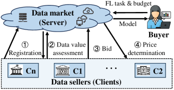
Figure 1. FLMarket high-level system overview

3.1. High-Level System Overview

Our framework consists of three parties: Data market (Server), Data sellers (Clients) and Data buyers. A buyer publishes an FL training task with a budget and the data market groups a set of clients to perform the training task. Finally, the data market returns a trained model to the buyer. Figure 1 presents the overview of the FLMarket pricing framework: ① seller first registers the FL task; ② the data market evaluates the data value of each client and returns an assessed price; ③ clients make bids (quote) for contributing their data; ④ the data market finalizes the price for the clients.

The pricing process consists of three steps: 1) evaluate data for each client by aggregating and getting global data distribution with a privacy-aware secret-sharing (PASS) protocol (see §4); 2) send score function to the clients for computation; 3) receive the scores back at the server. In principle, the clients with unseen classes and sufficient data volume have higher pricing and are regarded as high-quality clients.

Assumptions. We target cross-silo FL scenarios across organizations such as healthcare (Dayan et al., 2021) and finances (Basu et al., 2021). We assume that the participants would follow the protocols and refrain from modifying the data or sharing incorrect information with the server (Zhang et al., 2021a; Bonawitz et al., 2017) since such malicious activities would be quickly detected. On the other hand, the aggregation of individual class distribution would lead to privacy leakage as they often reveal sensitive information such as attribute percentage (Zhang et al., 2021a), personal habits (Deshpande and Karypis, 2004), sales record (Hartmann et al., 2023) and financial status (Chen and Ohrimenko, 2023). We aim to design an integrated pricing and privacy-preserving framework to resolve the tension between data privacy and data pricing.

3.2. Single-Client Evaluation

We evaluate individual client data based on their contribution to the FL training, which is assessed by a score function.

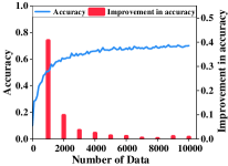
(a) Data quantity

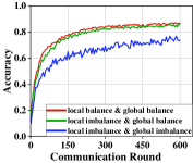
(b) Data balance

Figure 2. The impact of data quantity and distribution for FL training: a) An incremental increase of 1,000 data points has shown a diminishing rate of improvement in global accuracy; b) Imbalanced categories in both local and global data result in the worst performance.

Motivational Example. To evaluate data quality before training, a common technique is based on statistical information (Deng et al., 2021b; Saha et al., 2022; Li et al., 2021). For FL tasks, we consider two major factors of data quantity and class distribution by evaluating their impact on testing accuracy in Figure 2.

Observation 1: The contribution from client’s data increases regarding the data size but with diminishing marginal values. Figure 2a shows that the test accuracy climbs up with the increase of training data. However, $\Delta Accuracy$ drops rapidly, indicating that the contribution from data amount to test accuracy is marginal as the data amount increases.

Observation 2: Clients with data in scarce categories can significantly improve the overall FL accuracy. Figure 2b shows that local and global data imbalance significantly deteriorates the test accuracy. If the global data is balanced by bringing more clients with scarce categories (the green curve in Figure 2b), the accuracy degradation for FL training is much smaller. This aligns with the findings in (Wang et al., 2021a) that unseen categories help increase gradient diversity and improve model generalization.

Score Function. To calculate the score for each client, the server needs to obtain the data volume and categorical distribution from the clients in advance (privacy risks are addressed in Section 4). For class $c$ of $C$ categories, the $c$-class volume is represented as $n_{s}^{c}$. The total amount of data $N_{s}$ is the summation from all the classes: $N_{s}=\sum_{c=1}^{C}n_{s}^{c}$. Each client $e$ has the amount of $N_{e}$ data. For each class $c$ from the same set of $C$ categories, the volume of $c$ at client $e$ is denoted as $n_{e}^{c}$. As a result, we can define $N_{e}$ as the sum of volumes across all classes: $N_{e}=\sum_{c=1}^{C}n_{e}^{c}$. The score function on client $e$ is,

(1) $$\small u_{e}=\sum_{c=1}^{C}\theta_{c}\cdot\phi(n_{e}^{c}),$$

where $\theta_{c}$ represents the unique coefficient for this category and $\phi(\cdot)$ models the relation between input data and model accuracy. The score function can be interpreted as the sum of the $\phi(\cdot)$ function, with the data volume of each category as the input, weighted by $\theta_{c}$ for the different categories.

$\phi(\cdot)$ is formalized as equation 2.

(2) $$\small\begin{split}\phi(x)=\sum_{t=1}^{x}f({\rho(t)})\qquad s.t.\quad\rho(t)=\min(t/\alpha,1),\end{split}$$

where $x$ takes the value of $n_{e}^{c}$ for each client and $\rho(\cdot)$ is the normalising function, constrained within the range of $(0,1]$. $\alpha$ is a threshold parameter with $\alpha=N_{s}/(E\cdot C)$, which is the average data volume for each category across all the clients. If $n_{e}^{c}>\alpha$, we consider that an increase in data volume $n_{e}^{c}$ does not provide additional benefits, which aligns with Observation 1 in Section 3.1.

To model the relationship between data volume and accuracy, we draw inspiration from (Ben-David et al., 2010) and empirical observations (Kaplan et al., 2020), which suggest an $O(\log(x))$ contribution of data volume to accuracy. Consequently, we use the negative natural logarithm $-\ln(\cdot)$ as the function $f(\cdot)$ to map data volume to accuracy. The rationale behind the choice of $f(\cdot)$ is detailed in Appendix D.

For the coefficient $\theta_{c}$, it can be calculated as:

(3) $$\small\theta_{c}=1-n_{s}^{c}/N_{s}.$$

It reflects that if a category is relatively scarce in the global distribution, its weighted coefficient would be higher, which satisfies the demands from Observation 2.

3.3. Reaching a Consensus Price between Client and Server

As a data market, we should satisfy both data sellers and buyer. The score function computes a value for each client which meets server’s requirements. To satisfy clients requirements while ensuring the payments are within the given budget, we propose a second-phase pricing mechanism as follows.

Bidding Mechanism. We incorporate the design of the classical bidding mechanism (McAfee and McMillan, 1987; Lin et al., 2021; Zheng et al., 2016), where the server $S$ orchestrates the bidding procedures with the budget $R$. A client pool $\mathbb{E}$ consists of $E$ clients. The bidding procedures are designed to choose the most valuable clients within the budget constraint of $R$. We break down the bidding mechanism into two parts: winner selection and payment determination. Specifically, at the beginning of the bidding, client $e$ decides the bid $b_{e}$ according to the evaluation score and the potential cost of the task. The set of bids of $E$ clients is $\mathbb{B}=\{b_{e}\}_{e\in\mathbb{E}}$. The server selects the winning clients to join the task with the budget constraints $R$. And then decide the final payment $p_{e}$ for each winner $e$ with budget constraints.

Winner Selection. The procedure of the winner selection part is detailed in Algorithm 1 line 1-1. First, the server sorts clients by their score per bid and gets the list $\mathbb{V}$. Then, the server selects the winners in the order of $\mathbb{V}$. In particular, only clients with bids $b_{e}$ smaller than the budget constraint condition $\frac{R}{2}\cdot\frac{u_{e}}{U(\mathbb{S}_{k}\cup\{e\})}$, $e$ are eligible as a winner, a criterion also adopted in  (Zheng et al., 2016). If a client’s bid exceeds this constraint, the winner selection process terminates, and subsequent clients are not considered as winners.

Payment Determination. After the winners are selected, the server determines the payments for each of them. The basic idea of the payment determination can be described as follows. For each winner $e$, we consider a new list $\mathbb{V}^{-e}$ which eliminates the client $e$ from $\mathbb{V}$. Select winners from the list $\mathbb{V}^{-e}$ similar to the winner selection part. We assume that client $e$ replaces client $j$ as the winner in list $\mathbb{V}^{-e}$ and calculate the maximum bid $p_{e(j)}^{\prime}$ at which $e$ can win the auction in position $j$. However, each $j$ corresponds to a different $p_{e(j)}^{\prime}$. Hence, we take the maximum value of $p_{e(j)}^{\prime}$ as the final payment for $e$.

The procedure of the payment determination part is detailed in Algorithm 1 line 1-1. Similar to the winner selection, we select the client in order of list $\mathbb{V}^{-e}$. Then compute the maximum bid $p_{e(j)}^{\prime}$ that client $e$ can provide to win the auction in list $\mathbb{V}^{-e}$. The bid $b_{e(j)}$ should satisfy two conditions.

• Client $e$ should have more larger score per bid than $j$, i.e.,

  (4) $$\frac{u_{e}}{b_{e(j)}}\geq\frac{u_{j}}{b_{j}}\Rightarrow b_{e(j)}\leq\frac{u_{e}\cdot b_{j}}{u_{j}}=\lambda_{e(j)}.$$

• The bid of client $e$ should satisfy the budget constraint condition, i.e.,

  (5) $$b_{e(j)}\leq\frac{R}{2}\cdot\frac{u_{e}}{U(\mathbb{S}_{j-1}^{\prime}\cup\{e\})}=\beta_{e(j)}.$$

We set $\hat{k}$ as the smallest index which satisfies the budget constraint in $\mathbb{V}^{-e}$, i.e., $b_{\hat{k}+1}>\frac{R}{2}\cdot\frac{u_{\hat{k}+1}}{U(\mathbb{S}_{\hat{k}+1}^{\prime})}$. Therefore, the maximum index in $\mathbb{V}^{-e}$ that $e$ can replace as the winner is $\hat{k}+1$. Since the bid should satisfy both of the above two conditions, we get the maximum of the bid is $p_{e(j)}^{\prime}=\min\{\lambda_{e(j)},\beta_{e(j)}\}$. In Inequality (4), the value of $\lambda_{e(j)}$ monotonically decreases with the index $j$. In Inequality (5), the value of $\beta_{e(j)}$ is dynamically changing with $j$. Therefore, we determine the maximum of $p_{e(j)}^{\prime}$ in different $j$ for $j\in[1,\hat{k}+1]$ as the final payment. i.e., $p_{e}=\max_{1\leq j\leq\hat{k}+1}\{p_{e(j)}^{\prime}\}$.

1

2 Input: Candidate clients $\mathbb{E}$, Budget $R$, Bids $\mathbb{B}=\{b_{e}\}_{e\in\mathbb{E}}$ and scores $\mathbb{U}=\{u_{e}\}_{e\in\mathbb{E}}$

3 Output: Selected clients $\mathbb{S}_{k}$ and Payment $\mathbb{P}$

4 Winner Selection:

5 Sort according score per bid get $\mathbb{V}$: $\frac{u_{1}}{b_{1}}\geq...\geq\frac{u_{e}}{b_{e}}\geq...\geq\frac{u_{E}}{b_{E}}$

6 $\mathbb{S}_{k}\leftarrow\emptyset$; $U(\mathbb{S}_{k})=\sum_{e\in\mathbb{S}_{k}}u_{e}$

7 for $\frac{u_{e}}{b_{e}}$ in $\mathbb{V}$ do

8       if $b_{e}>\frac{R}{2}\cdot\frac{u_{e}}{U(\mathbb{S}_{k}\cup\{e\})}$ then

9             break;

10       end if

11      $\mathbb{S}_{k}\leftarrow\mathbb{S}_{k}\bigcup\{e\}$;

12      

13 end for

14 Payment Determination:

15 for $e$ in $\mathbb{S}_{k}$ do

16       $j\leftarrow 1$; $\mathbb{S}_{j-1}^{\prime}\leftarrow\emptyset$; $p_{e}\leftarrow 0$; $\mathbb{V}^{-e}$: $\frac{u_{1}}{b_{1}}\geq...\geq\frac{u_{E-1}}{b_{E-1}}$

17       for $\frac{u_{j}}{b_{j}}$ in $\mathbb{V}^{-e}$ do

18             if $b_{j}>\frac{R}{2}\cdot\frac{u_{j}}{U(\mathbb{S}_{j-1}^{\prime}\cup\{j\})}$ then

19                   break;

20             end if

21            $\lambda_{e(j)}\leftarrow\frac{u_{e}\cdot b_{j}}{u_{j}}$; $\beta_{e(j)}\leftarrow\frac{R}{2}\cdot\frac{u_{e}}{U(\mathbb{S}_{j-1}^{\prime}\cup\{e\})}$;

22             $p_{e(j)}^{\prime}=\min\{\lambda_{e(j)},\beta_{e(j)}\}$; $p_{e}=\max\{p_{e},p_{e(j)}^{\prime}\}$;

23             $\mathbb{S}_{j}^{\prime}\leftarrow\mathbb{S}_{j-1}^{\prime}\bigcup\{j\}$; $j\leftarrow j+1$

24            

25       end for

26      $\lambda_{e(j)}\leftarrow\frac{u_{e}\cdot b_{j}}{u_{j}}$; $\beta_{e(j)}\leftarrow\frac{R}{2}\cdot\frac{u_{e}}{U(\mathbb{S}_{j-1}^{\prime}\cup\{e\})}$;

27       $p_{e}\leftarrow\max\{p_{e},\min\{\lambda_{e(j)},\beta_{e(j)}\}\}$;

28      

29 end for

30$\mathbb{P}=\{p_{e}\}_{e\in\mathbb{S}_{k}}$

31 return $\mathbb{S}_{k}$ and $\mathbb{P}$

Algorithm 1 Budget-constrained Pricing Mechanism

A Walk-Through Example. Consider an example with a client pool of $E=4$ clients and a budget constraint $R=140$. The scores and bids of all clients in $\mathbb{E}$ is $\mathbb{U}=\{5,6,10,20\}$ and $\mathbb{B}=\{10,13,80,45\}$. Then calculate each score per bid and sort clients get list $\mathbb{V}$:

$$\{\frac{u_{1}}{b_{1}}:\frac{5}{10}=0.5;\frac{u_{2}}{b_{2}}:\frac{6}{13}=0.46;\frac{u_{3}}{b_{3}}:\frac{20}{45}=0.44;\frac{u_{4}}{b_{4}}:\frac{10}{80}=0.125\}$$

Sequential client selection according to list $\mathbb{V}$, we get

$$b_{1}<\frac{R}{2}\frac{u_{1}}{U(\emptyset\cup\{1\})}=70;\quad b_{2}<\frac{R}{2}\frac{u_{2}}{U(\{1\}\cup\{2\})}=38.2;$$

$$b_{3}<\frac{R}{2}\frac{u_{3}}{U(\{1,2\}\cup\{3\})}=45.2;\quad b_{4}>\frac{R}{2}\frac{u_{4}}{U(\{1,2,3\}\cup\{4\})}=17.1.$$

Since $b_{4}>\frac{R}{2}\cdot\frac{u_{4}}{U(\{1,2,3\}\cup\{4\})}$, the winner set $\mathbb{S}_{k}=\{1,2,3\}$. Then the server determines the payments for them. For client $1$, $\mathbb{V}^{-1}:\{\frac{u_{2}}{b_{2}};\frac{u_{3}}{b_{3}};\frac{u_{4}}{b_{4}}\}$, then we select clients from $\mathbb{V}^{-1}$ one by one until violate budget constraints. Client {2,3} satisfy the budget constraints in $\mathbb{V}^{-1}$. When select to client $2$,

$$\lambda_{1(2)}=\frac{u_{1}\cdot b_{2}}{u_{2}}=10.9;\beta_{1(2)}=\frac{140}{2}\times\frac{u_{1}}{0+u_{1}}=70;p_{1(2)}^{\prime}=10.9.$$

Similarly, $p_{1(3)}^{\prime}=\min\{11.4,31.8\}=11.4$, $p_{1(4)}^{\prime}=\min\{40,11.3\}=11.3$. Then the final payment of client $1$ is $p_{1}=p_{1(3)}^{\prime}=11.4$. Similar to the client $1$, we calculate each winner payment $p_{2}=p_{2(3)}^{\prime}=13.6$, $p_{3}=p_{3(4)}^{\prime}=45.2$. And the total payment is $70.2<R$.

Property of the Mechanism. A reasonable bidding mechanism needs to satisfy Truthful, Individual Rationality, and Budget Constraints. Next, we prove our mechanism satisfies these properties.

Theorem 3.1.

A bidding mechanism is truthful if and only if (Singer, 2010):

1. The selection algorithm is monotone, i.e. if $e$ wins the bidding by $b_{e}$, it would also win by bidding $b_{e}^{\prime}<b_{e}$;

2. Each winner is paid at the critical value: $e$ would not win the bidding if $b_{e}^{\prime}>p_{e}$.

Lemma 3.2.

The algorithm for winner selection is monotone.

Proof.

The proof is given in the Appendix E.1 ∎

Lemma 3.3.

The payment $p_{e}\in\mathbb{P}$ is the critical price of auction winner $e\in\mathbb{S}_{k}$.

Proof.

The proof is given in the Appendix E.2 ∎

Theorem 3.4.

The bidding mechanism is Truthful.

Proof.

According to the Lemmas 3.2, 3.3 and Theorem 3.1, our bidding mechanism satisfies the monotone and the final payment is the critical price. Thus, the bidding mechanism is Truthful. ∎

Theorem 3.5.

The auction satisfies Individual Rationality.

Proof.

If the payment for client $e$ is larger than its bid $b_{e}$, the auction is Individual Rationality. let’s compare the bid $b_{e}$ with $p_{e(\gamma)}^{\prime}$, where the index $\gamma$ in $\mathbb{V}^{-e}$ is same with $e$ in $\mathbb{V}$. Therefore, the winners before $e$ in $\mathbb{V}$ is same with the winners before $\gamma$ in $\mathbb{V}^{-e}$. We know the payment for client $e$ is the maximum over all possible $p_{e(j)}^{\prime}$ for $j\in[1,\hat{k}+1]$, thus $p_{e(\gamma)}^{\prime}\leq p_{e}$. According to the winner selection part, we know $b_{e}$ satisfied the budget constraint, i.e.,

(6) $$b_{e}\leq\frac{R}{2}\cdot\frac{u_{e}}{U(\mathbb{S}_{e-1}\cup\{e\})}=\frac{R}{2}\cdot\frac{u_{e}}{U(\mathbb{S}_{\gamma-1}^{\prime}\cup\{e\})}=\beta_{e(\gamma)}.$$

In list $\mathbb{V}$, $\gamma$ is behind $e$ then we get

(7) $$\frac{u_{e}}{b_{e}}\geq\frac{u_{\gamma}}{b_{\gamma}}\Rightarrow b_{e}\leq\frac{u_{e}\cdot b_{\gamma}}{u_{\gamma}}=\lambda_{e(\gamma)}.$$

Recall that $p_{e(\gamma)}^{\prime}\leq p_{e}$ and according to inequalities (6,7), we get $b_{e}\leq\min\{\lambda_{e(\gamma)},\beta_{e(\gamma)}\}=p_{e(\gamma)}^{\prime}\leq p_{e}$. Therefore, the payment for the winner $e$ is always larger than its bid $b_{e}$ and the auction is Individual Rationality. ∎

Lemma 3.6.

For clients set $\mathbb{S}_{1}\subset\mathbb{S}_{2}\subseteq\mathbb{S}$, if $\hat{e}=\arg\max_{e\in\mathbb{S}_{2}\setminus\mathbb{S}_{1}}\frac{u_{e}}{b_{e}}$ then the following inequality is valid.

(8) $$\frac{U(\mathbb{S}_{2})-U(\mathbb{S}_{1})}{\sum_{i\in\mathbb{S}_{2}}b_{i}-\sum_{j\in\mathbb{S}_{1}}b_{j}}<\frac{u_{\hat{e}}}{b_{\hat{e}}}$$

Proof.

The proof is given in the Appendix E.3. ∎

Theorem 3.7.

The mechanism is within the budget constraint.

Proof.

We try to show that the auction satisfies the budget constraint by proving that the upper bound of the payment $p_{e}$ is $\frac{u_{e}}{U(\mathbb{S}_{k})}R$. We prove it by contradiction, assume $p_{e}>\frac{u_{e}}{U(\mathbb{S}_{k})}R$. According to the payment determination mechanism above, we know the payment $p_{e}$ satisfies the following conditions:

(9) $$p_{e}\leq\frac{u_{e}\cdot b_{r}}{u_{r}}\qquad p_{e}\leq\frac{R}{2}\frac{u_{e}}{U(\mathbb{S}_{r-1}^{\prime}\cup\{e\})}$$

Since $e$ is the $e$-th winner, thus for $j\in[1,e-1]$, $b_{e}>\lambda_{e(j)}$. We know that $p_{e(j)}^{\prime}\leq\lambda_{e(j)}$, then we get $b_{e}>\lambda_{e(j)}\geq p_{e(j)}^{\prime}$. In Theorem 3.3 we prove the bid of $e$ is no larger than the final payment, i.e., $b_{e}\leq p_{e}$. Therefore, we get the inequality:

(10) $$p_{e(j)}^{\prime}<b_{e}\leq p_{e}=p_{e(r)}^{\prime},\quad j\in[1,e-1]$$

From the Inequality (10) we know $r$ is not in list $[1,e-1]$, so $r$ is behind $e$ and we have $\mathbb{S}_{e-1}\subseteq\mathbb{S}_{r-1}^{\prime}$. Let’s consider the following two scenarios:

• $\mathbb{S}_{r-1}^{\prime}\bigcup\{e\}=\mathbb{S}_{r-1}^{\prime}\bigcup\mathbb{S}_{k}$. Since $\mathbb{S}_{e-1}\subseteq\mathbb{S}_{r-1}^{\prime}$, the Inequality (9) can be rewritten as:

  (11) $$\frac{u_{e}}{p_{e}}\geq\frac{2U(\mathbb{S}_{r-1}^{\prime}\bigcup\{e\})}{R}=\frac{2U(\mathbb{S}_{r-1}^{\prime}\bigcup\mathbb{S}_{k})}{R}\geq\frac{2U(\mathbb{S}_{k})}{R}$$

  Therefore, according to Inequality (11) we get $p_{e}\leq\frac{u_{e}}{U(\mathbb{S}_{k})}\cdot R$ which contradicts the assumption. Thus the assumption is not valid.

• $\mathbb{S}_{r-1}^{\prime}\bigcup\{e\}\subset\mathbb{S}_{r-1}^{\prime}\bigcup\mathbb{S}_{k}$. Set $\mathbb{S}_{1}=\mathbb{S}_{r-1}^{\prime}\bigcup\{e\},\mathbb{S}_{2}=\mathbb{S}_{r-1}^{\prime}\bigcup\mathbb{S}_{k}$ and $\mathbb{S}_{1}\subset\mathbb{S}_{2}$. Assume $\hat{r}=\arg\max_{t\in\mathbb{S}_{2}\setminus\mathbb{S}_{1}}\frac{u_{t}}{b_{t}}$, according to the Inequalities (8,9) and Lemma 3.6 we get:

  (12) $$\frac{U(\mathbb{S}_{2})-U(\mathbb{S}_{1})}{\sum_{i\in\mathbb{S}_{2}}b_{i}-\sum_{j\in\mathbb{S}_{1}}b_{j}}<\frac{u_{\hat{r}}}{b_{\hat{r}}}\leq\frac{u_{e}}{p_{e}}$$

  Since we previously assume $p_{e}>\frac{u_{e}}{U(\mathbb{S}_{k})}\cdot R$, thus $\frac{u_{e}}{p_{e}}<\frac{U(\mathbb{S}_{k})}{R}$. We know that $b_{e}\leq p_{e}\leq\frac{R}{2}\frac{u_{e}}{U(\mathbb{S}_{r-1}^{\prime}\cup\{e\})}$ (Inequality 9). Then:

  (13) $$\frac{u_{e}}{b_{e}}\geq\frac{2U(\mathbb{S}_{r-1}^{\prime}\cup\{e\})}{R}\Rightarrow\frac{u_{k}}{b_{k}}\geq\frac{2U(\mathbb{S}_{k})}{R}$$

  According to the Inequality (13), we can get inequality as follows.

  (14) $$\frac{u_{1}}{b_{1}}\geq\frac{u_{2}}{b_{2}}\geq\dots\geq\frac{u_{k}}{b_{k}}\geq\frac{2U(\mathbb{S}_{k})}{R}$$

  Then we get $b_{e}\leq\frac{R}{2}\cdot\frac{u_{e}}{U(\mathbb{S}_{k})}$, then $\sum_{e\in\mathbb{S}_{k}}b_{e}\leq\frac{R}{2}\cdot\frac{\sum_{e\in\mathbb{S}_{k}}u_{e}}{U(\mathbb{S}_{k})}=\frac{R}{2}$. Therefore, we can get :

  (15) $$\sum_{i\in\mathbb{S}_{2}}b_{i}-\sum_{j\in\mathbb{S}_{1}}b_{j}=\sum_{e\in\mathbb{S}_{2}\setminus\mathbb{S}_{1}}b_{e}\leq\sum_{e\in\mathbb{S}_{k}}b_{e}\leq\frac{R}{2}$$

  Recall that $\mathbb{S}_{2}=\mathbb{S}_{r-1}^{\prime}\bigcup\mathbb{S}_{k}$, thus $\mathbb{S}_{k}\subseteq\mathbb{S}_{2}$. Then we get the Inequality (16).

  (16) $$\frac{2(U(\mathbb{S}_{k})-U(\mathbb{S}_{1}))}{R} \leq\frac{2(U(\mathbb{S}_{2})-U(\mathbb{S}_{1}))}{R}$$

  $$\leq\frac{U(\mathbb{S}_{2})-U(\mathbb{S}_{1})}{\sum_{e\in\mathbb{S}_{2}\setminus\mathbb{S}_{1}}b_{e}}\leq\frac{u_{e}}{p_{e}}<\frac{U(\mathbb{S}_{k})}{R}$$

  Then we can deduce from the above inequality that $2(U(\mathbb{S}_{k})-U(\mathbb{S}_{1}))<u(\mathbb{S}_{k})$. Thus

  (17) $$U(\mathbb{S}_{k})<2U(\mathbb{S}_{1})=2U(\mathbb{S}_{r-1}^{\prime}\cup\{e\})$$

  $$\Rightarrow \frac{u_{e}}{p_{e}}\geq\frac{2U(\mathbb{S}_{r-1}^{\prime}\cup\{e\})}{R}\geq\frac{U(\mathbb{S}_{k})}{R}$$

  From the inequality above, we can conclude that $p_{e}\leq\frac{u_{e}}{U(\mathbb{S}_{k})}\cdot R$ which contradicts the assumption.

Therefore, the assumption is invalid and the upper bound of the payment is $\frac{u_{e}}{U(\mathbb{S}_{k})}\cdot R$. So, $\sum_{e\in\mathbb{S}_{k}}p_{e}\leq\frac{\sum_{e\in\mathbb{S}_{k}}u_{e}}{U(\mathbb{S}_{k})}\cdot R=R$, satisfying budget constraints. ∎

4. Privacy-aware Secret-sharing Mechanism

In this section, we first discuss the design idea and primitives for the PASS protocol in § 4.1. Then, in § 4.2 we introduce the implementation of PASS for obtaining the global data distribution. Finally, we analyse the security of the proposed protocol.

4.1. Design of PASS

Main Idea. To protect the sensitive information of clients, we leverage the Diffie-Hellman key agreement (Hellman, 1976) and distribution aggregation method to generate a pair of positive and negative random noises to obfuscate the local data distribution before sharing them with the server. Thereafter, we sum up these obfuscated local distributions and the added noises can be cancelled out, reminding the global distribution. To be precise, we construct a random seed based on key pairs $(SK_{e},PK_{v})$ in client $e$ and $(SK_{v},PK_{e})$ in client $v$, which the public keys $PK_{e},PK_{v}$ are distributed by client $e$ and $v$ respectively. Using the above key pairs, we can generate the same random seed $s_{e,v}$, which can be used to generate a noise by a pseudorandom generator (PRG) (Yao, 1982) for both client $e$ and $v$, i.e., $PRG(s_{e,v})$. The $PRG(s_{e,v})$ that has the same dimensions as the host clients’ local distribution (i.e., $|\mathbb{N}_{e}|==|PRG(s_{e,v})|$ and $|\mathbb{N}_{v}|==|PRG(s_{e,v})|$) will be added to $\mathbb{N}_{e}$ and $\mathbb{N}_{v}$. Therefore, we develop a distribution aggregation method that constructs a pair of positive and negative of noises, which can be cancelled after aggregation on the server side.

Key Agreement. In this paper, we use Diffie-Hellman key agreement to achieve pairwise clients agreeing on a random seed that not be disclosed by the server or clients. The key agreement consists of a tuple of algorithms ($KA.param,KA.gen,KA.agree$). $KA.param(r)\\ \rightarrow R$ generate a public parameter $R$ based on the security parameter $r$. $KA.gen(R)\rightarrow(SK,PK)$ uses the public parameter $R$ to produce a private-public key pair, and $KA.agree(SK_{e},PK_{v})\rightarrow s_{e,v}$ can generate the identical private shared key $s_{e,v}$ using the private key of $e$ and public key of $v$ which are generated from the same public parameter $R$. As a result, we can have two key pairs that generate the same random seed, i.e., $KA.agree(SK_{e},PK_{v})=KA.agree(SK_{v},PK_{e})=s_{e,v}$.

Distribution Aggregation. We assume that each client $e\in\mathbb{E}$ possesses a $C$-dimensional private vector $\mathbb{N}_{e}=\{n_{e}^{c}\}_{c\in\{1,...,C\}}$ indicating their local data distribution. The proposed secret share method aims to enable the server $S$ to securely compute global data distribution $\mathbb{N}_{s}=\sum_{e\in\mathbb{E}}\mathbb{N}_{e}$ without accessing the private local distributions $\mathbb{N}_{e}$.

We first assign each client $e$ a unique identifier from {$1$ to $E$}, pairing all clients in a pairwise manner, denoted as $(e,v)$. Then, we use the PRG to generate the identical random vectors $PRG(s_{e,v})$ based on the random seed $s_{e,v}$. Furthermore, we introduce the $\epsilon_{e,v}$ to determine whether to add or subtract random vectors $PRG(s_{e,v})$. When $e$ is less than $v$ (i.e., $e<v$), the $\epsilon_{e,v}$ equals to 1. On the contrary, if $e$ is greater than $v$ (i.e., $e>v$), the $\epsilon_{e,v}$ equals to -1. Thereafter, we use Equation (18) to compute an alternative distribution of $\mathbb{N}_{e}$ (i.e., $\mathbb{Y}_{e}$) by adding all $\epsilon_{e,v}\cdot PRG(s_{e,v})$ generated by client $e$ paired with other clients $v\in\mathbb{E}$ to avoid $\mathbb{N}_{e}$ being disclosed.

(18) $$\small\mathbb{Y}_{e}=\mathbb{N}_{e}+\sum_{v\in\mathbb{E}}\epsilon_{e,v}\cdot PRG(s_{e,v});\;\epsilon_{e,v}=\left\{\begin{aligned} 1&\hskip 14.22636pte<v\\ -1&\hskip 14.22636pte>v\end{aligned}\right.$$

Once the server $S$ obtains all $\mathbb{Y}_{e}$, the global data distribution $\mathbb{N}_{s}$ can be computed via Equation (19), where the added $PRG(s_{e,v})$ are cancelled each other out, reminding the global data distribution $\mathbb{N}_{s}$.

(19) $$\small\mathbb{N}_{s}=\sum_{e\in\mathbb{E}}\mathbb{Y}_{e}=\sum_{e\in\mathbb{E}}[\mathbb{N}_{e}+\sum_{v\in\mathbb{E}}\epsilon_{e,v}\cdot PRG(s_{e,v})]=\sum_{e\in\mathbb{E}}\mathbb{N}_{e}$$

4.2. The PASS Protocol

Table 4 in appendix F shows the protocol of the $PASS$ to aggregate data distribution from clients. In step 1, each client uses the given security parameters $r$ to generate the public parameters $R$. Then, client $e$ uses $R$ to generate key pairs $(PK_{e},SK_{e})$. After that, client $e$ sends its public key $PK_{e}$ to the server. The server received $PK_{e,e\in\mathbb{E}}$ from each client, and the server broadcast $(PK_{e},e)$ to each client when received all $PK_{e}$.

In step 2, client $e$ received all $PK_{v}$ and its client identifier $v$ from the server. Then, it uses $PK_{e}$ and the private key $SK_{e}$ to generate random seed $s_{e,v}$ through the $KA.agree$ algorithm. Based on $s_{e,v}$, a $C$-dimensional random vector $\mathbb{RV}_{e,v}\leftarrow\epsilon_{e,v}\cdot PRG(s_{e.v})$ is generated via PRG, where $\epsilon_{e,v}=1$ if $e<v$ and $\epsilon_{e,v}=-1$ if $e>v$. Then, the client $e$ adds the local distribution $\mathbb{N}_{e}$ with all $\mathbb{RV}_{e,v}$ to obtain the pseudo local data distribution $\mathbb{Y}_{e}$ and then sends it to the server. The server sums all $\mathbb{Y}_{e}$ from all client $e\in\mathbb{E}$ to get the global distribution $\mathbb{N}_{s}$ when receiving all $\mathbb{Y}_{e}$. Finally, the server broadcasts $\mathbb{N}_{s}$ to all clients for data evaluation. A running example of $PASS$ is included in appendix F.

Performance and Security Analysis. The communication complexity of each client and server is $O(E)$ and $O(E^{2})$, respectively. This arises from each client’s requirement to receive public keys from the other $E-1$ clients. For communication costs, the actual communication cost is negligible compared to FL training since the size of the keys is much smaller than the weights of the model. Additionally, the PASS can protect the clients’ privacy in the semi-honest client environment. The detailed analysis of the communication cost and security is shown in Appendix J and  G.

5. Evaluation

In this section, we evaluate the impact of the client selection on the subsequent FL training accuracy by comparing FLMarket to four state-of-the-art pre-training client selection methods. In addition, we compared FLMarket with an in-training client selection algorithm, which can effectively use the training feedback. Experimental results show that, FLMarket outperforms other state-of-the-art pre-training client selection methods in most cases. Even when compared to the in-training client selection algorithm, FLMarket still achieves competitive accuracy with less runtime overhead.

5.1. Experimental Setup

Applications, Datasets and Models. We evaluate FLMarket in two applications: Image Classification (IC) and Human Activity Recognition (HAR). For IC, we utilize the CIFAR-10 (Krizhevsky et al., 2009) and CINIC-10 (Darlow et al., 2018) datasets with a ResNet-56 (He et al., 2016) model. For HAR, we employ the DEAP dataset (Koelstra et al., 2011) using peripheral physiological signals and train a three-layer CNN model on it.

FL Training Set Up. We evaluated FLMarket under different numbers of clients, including both 20 and 100 clients. Each client’s data distribution is generated through a two-step process. Firstly, we adjust the global data distribution by randomly pruning data from different classes to achieve an unbalanced global distribution. In the second step, based on the different global data distributions, we allocate data for each class to each client following a Dirichlet distribution ($\alpha=0.5$) for simulating Non-i.i.d. scenarios (Hsu et al., 2019; Li et al., 2022; Lin et al., 2020). Appendix H shows the example of the generated dataset on CIFAR-10. In summary, our evaluation encompasses three datasets, each tested under three selection ratios and six distributions (seven distributions for CINIC-10), resulting in a total of 57 test cases. We trained all FL tasks for 600 rounds, with an initial learning rate of 0.001 for CINIC-10 and 0.003 for CIFAR-10 and DEAP.

Baselines. FLMarket focuses on pre-training data evaluation in a more challenging setting, where no direct feedback is available from the training process. To align with this focus, we selected four primary baseline methods: random selection (RS), quantity-based selection (QBS) (Zeng et al., 2020), DICE (Saha et al., 2022), and diversity-driven selection (DDS) (Li et al., 2021), all of which are based on pre-training data evaluation. It is worth noting that, while more recent works on model-based evaluation methods exist (Li et al., 2023; Sun et al., 2022, 2024), these methods require training feedback and can only be applied during the FL training phase. FLMarket fundamentally differs from these methods but can be integrated with them since they target different phases. Therefore, we included an in-training client selection method for reference. A brief description of each baseline method is provided in Appendix I.

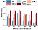
(a) 5 clients selected

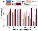
(b) 10 clients selected

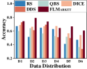
(c) 15 clients selected

Figure 3. CIFAR-10: $n$ clients selected from 20 clients

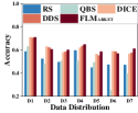
(a) 5 clients selected

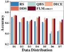
(b) 10 clients selected

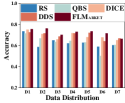
(c) 15 clients selected

Figure 4. CINIC-10: $n$ clients selected from 20 clients

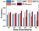
(a) 5 clients selected

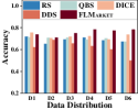
(b) 10 clients selected

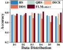
(c) 15 clients selected

Figure 5. DEAP: $n$ clients selected from 20 clients

5.2. Comparison with Pre-training Selection

We evaluate the performance of FLMarket on selecting clients by comparing the proposed algorithm with four pre-training client selection baselines. Figures 3, 4 and  5 show the final test accuracy of each baseline and FLMarket. It is observed that FLMarket outperforms other baselines (RS, QBS, DICE, DDS) in a wide range of data distributions across three datasets, particularly when the distribution is highly unbalanced (e.g., D4, D5, D6).

For CIFAR-10, FLMarket achieves up to 40.78 $\%$, 44.78 $\%$, 17.52 $\%$ and 47.05 $\%$ (all on D6 in 10 out of 20 selection) higher accuracy when compared to RS, QBS, DICE and DDS, respectively. In terms of CINIC-10, compared to four baselines, FLMarket has up to 28.10 $\%$ (on D6 in 10 out of 20 selection), 31.74 $\%$ (on D6 in 5 out of 20 selection), 5.44 $\%$ (on D5 in 15 out of 20 selection) and 7.27 $\%$ (on D6 in 15 out of 20 selection) higher accuracy, respectively. Regarding DEAP, Figure 5 shows that FLMarket achieves up to 25.67 $\%$ (on D4 in 5 out of 20 selection), 16.41 $\%$ (on D6 in 5 out of 20 selection), 8.63 $\%$ (on D6 in 5 out of 20 selection) and 29.21 $\%$ (on D6 in 5 out of 20 selection) higher accuracy than other baselines. As the data distribution becomes increasingly unbalanced (e.g., D4, D5 and D6), FLMarket exhibits significantly better accuracy than other baselines. This demonstrates FLMarket’s ability to mitigate the impact of global imbalance.

Among all the baselines, DICE exhibits the best performance. Nonetheless, FLMarket consistently outperforms DICE across three datasets and three different selection scenarios, with average accuracy improvements of 7.08 $\%$, 1.81 $\%$ and 3.53 $\%$ on CIFAR-10, CINIC-10 and DEAP respectively. Across all 57 tested distributions, FLMarket achieves the highest accuracy in 44 distributions (77%). For the most imbalanced distributions (D4, D5, and D6), FLMarket achieves the highest accuracy in 22 out of 27 test distributions (81%), highlighting its strength in handling imbalanced distributions. When the number of clients is scaled up to 100, FLMarket can still achieve better performance compared to the baselines (the experimental results are detailed in Appendix K).

Convergence speed. We compare the convergence rate of FLMarket with all the baseline methods. Figure 6 demonstrates that FLMarket exhibits significantly faster convergence and attains a lower training loss, consistently outperforming other approaches. In detail, FLMarket achieves an target accuracy of 0.6 after only approximately 130 rounds, while RS, QBS, DICE and DDS require 550, 350, 170 and 380 rounds, respectively. This results in a speedup of 4.23 $\times$, 2.69 $\times$, 1.31 $\times$, and 2.92 $\times$, respectively. We also observed similar conclusions in other datasets and distributions as well, where FLMarket exhibits faster convergence compared to other baselines. We also observed a similar speedup in latency for FLMarket in achieving the target accuracy. This outcome is expected, as FLMarket conducts pre-training data evaluation once before the training, thereby adding no computational overhead during the FL training process.

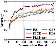
(a) Accuracy convergence

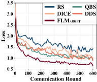
(b) Loss convergence

Figure 6. The accuracy and loss curves for FLMarket and other four baselines under the D1 distribution with a selection of 10 out of 20 clients on CIFAR-10 dataset.

The Data Distribution of Selected Clients. We further analyze the results of selected clients by comparing their data distributions. Specifically, we compare FLMarket to DICE under the selection of 10 out of 20 clients using the global distribution D6 of CIFAR-10. As shown in Table 1, both strategies select the same six clients from the client pool, namely, clients 2, 3, 7, 16, 17, and 19. However, in the disjoint selected clients, we observe that the clients chosen by FLMarket (i.e., 4, 8, 10, and 12) include data samples for all classes. In contrast, the clients selected by DICE (i.e., 1, 5, 13, and 18) missing some classes, i.e., classes 8, 9, and 10.

Although DICE also takes into account the impact of both data quantity and class distributions, it suffers issues: 1) it ignores that the marginal utility of data volume is decreased; 2) It only locally considers the class distribution instead of the global distribution. These designs result in DICE favouring clients with larger data quantities and smaller local variances. In contrast, FLMarket chooses clients with lower data quantities and global variance.

Table 1. Clients selected by FLMarket and DICE on distribution 6 of CIFAR-10 dataset

		C1	C2	C3	C4	C5	C6	C7	C8	C9	C10	Distribution
Overlapping	Client 2	9	203	19	224	224	318	362	40	0	0
	Client 3	5	120	112	311	472	58	0	319	360	0
	Client 7	6	125	66	14	207	75	6	97	121	36
	Client 16	151	378	29	4	85	44	125	12	69	174
	Client 17	30	42	171	201	11	1	322	111	53	70
	Client 19	33	212	23	99	29	64	141	109	157	25
FLMarket-specific	Client 4	220	11	2	46	659	0	55	16	169	143
	Client 8	401	11	56	6	724	66	36	5	25	6
	Client 10	1	244	13	93	4	83	52	191	1	25
	Client 12	287	9	42	65	13	5	114	600	45	21
	Sum	1143	1355	533	1063	2428	714	1413	1500	1000	500
DICE-specific	Client 1	530	38	59	349	33	346	209	0	0	0
	Client 5	281	174	211	4	247	570	0	0	0	0
	Client 13	257	159	37	13	125	628	180	0	0	0
	Client 18	2	605	43	133	166	271	398	0	0	0
	Sum	1304	2056	770	1342	1599	2345	1743	688	760	305
FLMarket	Data Number		11449		Variance		313880.1		Accuracy		77.28 $\%$
DICE			12912				431920.6				59.76 $\%$

5.3. Comparison with In-Training Selection

In-training client selection methods are impractical for pre-training pricing since they assess clients’ contributions during the FL training process. Nonetheless, we conducted a comparison on the accuracy between FLMarket and a popular in-training client selection method, namely S-FedAvg (Nagalapatti and Narayanam, 2021). S-FedAvg samples a subset of clients in each training round based on their Shapley values, which are calculated using their local accuracy. Figure 7 shows the test accuracy and average runtime latency for both FLMarket and S-FedAvg, with the selection of 5 clients out of 20 clients for all three datasets. It is worth noting that S-FedAvg sampled 5 clients in every training round, whereas FLMarket sampled 5 clients out of the 20 only once before the start of training.

Overall, FLMarket achieves an average of 66.12%, 61.75%, and 68.04% final accuracy over all data distributions compared to an average of 66.67%, 58.89%, and 64.17% on S-FedAvg. The results surprisingly demonstrate that FLMarket can achieve comparable or even better accuracy performance than the in-training client selection approach. FLMarket achieves better accuracy performances on more than half of the experiments. In terms of runtime overhead, FLMarket outperforms S-FedAvg significantly. Completing 600 rounds of training, S-FedAvg takes 603 minutes, 1354 minutes, and 223 minutes, which is 5 $\times$, 2.5 $\times$, and 11 $\times$ longer than FLMarket for the CIFAR-10, CINIC-10, and DEAP datasets, respectively.

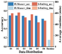
(a) CIFAR-10

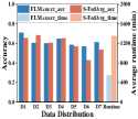
(b) CINIC-10

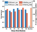
(c) DEAP

Figure 7. Comparison of performance between FLMarket and S-FedAvg across three datasets

In summary, compared to pre-training client selection baselines, FLMarket achieves an average improvement of 10.18% in accuracy across different datasets, data distributions, and selection modes. When compared to in-training client selection algorithms, FLMarket still achieves an average improvement of over 2.1% in accuracy and an average 3.16$\times$ speedup for per-round runtime latency.

6. Discussion

In this section, we discuss two challenges associated with deploying FLMarket in real-world FL data markets. It is worth noting that we do not focus on these challenges in the design of our framework because simple modifications or existing solutions can effectively mitigate them. Moreover, these solutions can be seamlessly integrated into our framework, thereby minimizing the impact of these challenges on our core contributions.

Dynamics of FL data market. Practical considerations, such as the constraints of truthfulness, individual rationality, and budget, have been integrated into the theoretical design of FLMarket. However, in real-world FL data markets, more advanced factors, such as market dynamics, may necessitate adaptive solutions for data pricing. For instance, rapid changes in client data or server budgets can influence optimal pricing outcomes. To address this, an adaptive re-launch mechanism can be incorporated into our framework, enabling the proposed bidding process to restart as needed to accommodate these variations.

Malicious attack. In designing label-sharing mechanisms, we propose the PASS protocol to prevent the leakage of label information. This protocol prevents the server from accessing sensitive client information. However, it does not guarantee protection against malicious clients who might provide false information or engage in fraudulent training to exploit rewards from the server. For instance, a common type of attack from malicious clients is the free-riding attack (Lin et al., 2019). To address this, existing in-training free-riding attack detection techniques (Wang et al., 2024, 2021b) can be integrated into our framework to mitigate these vulnerabilities. Based on the detection results, we can adjust the pre-training rewards to penalize malicious clients.

7. Conclusion

In this paper, we propose FLMarket, a privacy-preserved, pricing framework for pre-training client selection in federated learning. We design a truthful auction mechanism that is able to precisely determine the critical value and payment for the participating clients. Based on the aggregated class distribution, FLMarket incorporates a secure data evaluation function and selects high-quality clients while meeting the budget requirements. Extensive experiments demonstrate that FLMarket can evaluate the quality of local clients and select the best group of participants from the client pool, outperforming other baselines by a large margin.

APPENDIX

Appendix A Survey on the Impact of Pre-training Data Pricing on Participation Willingness in FL

In this section, we provide our empirical survey on how data pricing influences users’ willingness to participate in FL training. We first present our questionnaire and then provide a description of the participants. Based on the results collected, we then offer our analysis and conclusions, which highlight the significant importance of pre-training pricing in greatly enhancing the participation willingness of end users.

A.1. Questionnaire

Title. Questionnaire on Data Pricing in Federated Learning

Introduction. Welcome to our questionnaire! This survey aims to investigate how the pricing mechanism in federated learning (FL) influences users’ participation willingness.

First, we will provide some necessary background information on FL in case you are not familiar with it. Next, participants will be asked four multiple-choice questions about their thoughts on the pricing mechanism in FL. Please select the options that are most suitable for you.

FL Basics.

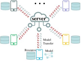
Figure 8. FL training architecture

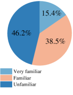
(a) Familiarity with FL

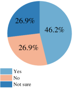
(b) Whether to join

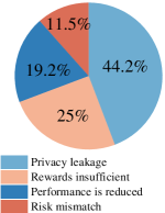
(c) Concerns in FL

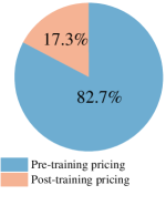
(d) More attractive mechanism

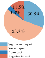
(e) Pre-training pricing impact

Figure 9. Results of the questionnaire

Table 2. Comparison of functional indicators between FLMarket with other frameworks

Functional indicators	FLMarket	AFL (Zhou et al., 2021)	AUCTION (Deng et al., 2021b)	DICE(Saha et al., 2022)	DDS (Li et al., 2021)	martFL(Li et al., 2023)	DEVELOP(Sun et al., 2022)	SARDA(Sun et al., 2024)
Pre-Training Auction and Incentive	✔	✔	✖	✖	✖	✖	✖	✖
Data Pricing and Client Selection	✔	✔	✖	✖	✖	✖	✖	✖
Privacy-aware Client Evaluation	✔	✖	✔	✔	✔	✔	✔	✔
Task Budget Control	✔	✖	✔	✖	✖	✖	✖	✖

Figure 8 provides a typical training architecture for FL. In FL training, your role is that of a client, holding your own data on personal devices such as smartphones. The server (e.g., companies) will distribute the training tasks to your smartphones and use your local resources to train a global model. Obviously, the training process will consume your personal resources, such as on-device computation and data communication. As compensation, the server will also offer rewards to the participating clients. FL is more privacy-preserving compared to traditional centralized training since no raw data is transmitted from your device to the server.

Multiple-Choice Questions.

Q1: Are you familiar with FL?

• Very familiar. I have extensive knowledge and experience in the FL.

• Familiar. I have some understanding of the FL.

• Unfamiliar. I have little to no understanding or experience in the FL.

Q2: After having a basic understanding of FL, would you like to join an FL task by using your mobile phone for half an hour? You will receive some monetary rewards.

• Yes, I want to try.

• No, I don’t want to try.

• I am not sure; I need more information to make my decision.

Q3: Which of the following concerns do you have when participating in FL tasks?

• Privacy leakage. I worry that the server might access my private data on my phone.

• The rewards are insufficient to cover the cost.

• Mobile phone performance is reduced. I worry that the training will negatively impact my phone’s performance.

• Risk mismatch. The server does not have corresponding costs for potential breaches, such as failing to compensate the client.

Q4: If you already have information about the training time and resource consumption, which of the following incentive mechanism would be more attractive to you for participating in FL training?

• Pre-training pricing. A pre-training reward is evaluated and promised before training (e.g., you are promised $10), and the final reward is adjusted after training based on the results.

• Post-training pricing. No pre-training rewards are provided, and the final reward is determined after training based on the results.

Q5: To what extent do you think a pre-training reward affects your willingness to participate in FL?

• A pre-training reward has a significant impact, changing my decision from not participating to participating.

• A pre-training reward has some impact, making participation more attractive.

• A pre-training reward has no impact.

• A pre-training reward has a negative impact, making me less likely to participate.

Participant selection. We distributed the questionnaire both in person at the campus and through online advertisements. To ensure a diverse range of participants, we deliberately targeted various groups, including students, teachers, researchers, and engineers.

A.2. Results Analysis

After 7 days of the survey, we collected a total of 53 questionnaires on five questions. Figure 9 displays pie charts of the options for these five questions. Despite gaining a basic understanding of FL, many participants seemed hesitant to join the FL training. As shown in Figure 9b, about 46.2% of the respondents expressed a positive willingness to participate, while 26.9% explicitly refused, and another 26.9% wanted more information before making a decision. This implies the importance of an incentive mechanism in FL to encourage more participation. Among all the concerns for joining FL training, privacy is the most important factor, with 44.2% of respondents choosing this option. The second most significant concern is the rewards, accounting for 25% of responses, as shown in Figure 9b. This highlights that privacy should be the top priority to secure more participants, and reasonable rewards serve as a good incentive.

We then asked participants about their thoughts toward pre-training rewards compared to traditional post-training rewards. The results clearly show that a pre-training rewards mechanism is more effective in encouraging participation in FL. As shown in Figure 9d, 82.7% of respondents find the pre-training pricing mechanism more attractive. This conclusion is further supported by Figure 9e, where 84.6% of respondents believe that pre-training pricing has a positive impact (either significant or some impact) on their decision to participate in FL.

These findings highlight that ensuring privacy and offering reasonable rewards are crucial to enhancing participation in FL training. Additionally, pre-training incentives are particularly effective in motivating participants.

Appendix B Comparing FLMarket with other FL data sharing Frameworks

Table 2 summarizes the set of functional indicators discussed in several recent papers, and outlines whether a framework supports a functional indicator or not.

Appendix C Notation

Table 3 summarizes notations used in this paper.

Table 3. Notations in FLMarket

Notation	Description
$\mathbb{T}$, $\mathbb{S}_{k}$, $\mathbb{E}$	FL task, selected clients, client pool
$\mathbb{N}_{s}$, $\mathbb{N}_{e}$	Global class distribution vector,
	Local class distribution vector for client $e$
$S$	Server
$E$	Total number of clients
$R$	The budget for task $\mathbb{T}$
$C$, $c$	Volume of classes in a data set, class $c$
$b_{e}$, $\mathbb{B}$	Bid(s) from client $e$ and all clients
$u_{e}$, $\mathbb{U}$	Score(s) for client $e$ and all clients
$\mathbb{V}$	list of all clients sorted by score per bid
$p_{e}$, $\mathbb{P}$	Second-stage price(s) for client $e$ and all selected clients
$N_{s}$, $N_{e}$	Volume of data for global, client $e$
$n_{s}^{c}$, $n_{e}^{c}$	Volume of data for class $c$ on global and class $c$ on client $e$
$\rho(\cdot),\alpha$	Normalization function, threshold parameter
$\theta_{c}$	Weighted coefficient of category
$\phi(\cdot)$	Data quantity function for each class $c$ on client $e$
$SK$, $PK$	Private key, public key
$s_{e,v}$	Random seed
$\epsilon_{e,v}$	Positive and negative sign
$r$,$R$	Security parameter, public parameter
$\mathbb{RV}$	Signed random vector
$\mathbb{Y}_{e}$	Pseudo data distribution for client $e$

Appendix D Choosing $f(\cdot)$ and $\theta_{c}$ in Evaluation Function

We use CIFAR-10 dataset to study the effectiveness of the score function ${u}_{e}$ as shown in Equation 1 (§2.2). We configure six different distributions from this dataset for our evaluation.

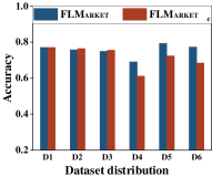
(a) Test accuracy with or without varying $\theta_{c}$

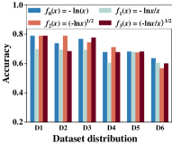
(b) Test accuracy with different $f(\cdot)$ functions

Figure 10. The impact of different category coefficients $\theta_{c}$ and $f(\cdot)$

The choice of $f(\cdot)$. $f(\cdot)$ represents the relationship between data volume and model accuracy. This relationship was previously formalized by Ben-David. et. al. (Ben-David et al., 2010) that the loss function scales at an $O(d\log(2m)/m)$ rate with respect to the sample size m as shown in lemma D.1. In addition, the scale laws in large language models also imply a similar logarithmic relation with diminishing returns of more training data (Kaplan et al., 2020). Therefore, we propose that the function $f(\cdot)$ should approximately follow this law.

Lemma D.1 ((Ben-David et al., 2010)).

Let $\mathcal{H}$ be a hypothesis space on $\mathcal{X}$ with VC dimension $d$. If $\mathcal{U}$ and $\mathcal{U}^{\prime}$ are samples of size $m$ from $\mathcal{D}$ and $\mathcal{D}^{\prime}$ respectively and $\hat{d}_{\mathcal{H}}(\mathcal{U},\mathcal{U}^{\prime})$ is the empirical $\mathcal{H}$-divergence between samples, then for any $\delta\in(0,1)$, with probability at least $1-\delta$,

(20) $$d_{\mathcal{H}}(\mathcal{D},\mathcal{D^{\prime}})\leq\hat{d}_{\mathcal{H}}(\mathcal{U},\mathcal{U}^{\prime})+4\sqrt{\frac{d\log(2m)+\log(\frac{2}{\delta})}{m}}$$

We also empirically evaluated four functions, including

$$f_{0}(x)=-\ln(x), \qquad f_{1}(x)=-\ln(x)/x$$

$$f_{2}(x)=\sqrt{-\ln(x)}, \qquad f_{3}(x)=\sqrt{-\ln(x)/x}$$

for scoring each clients. Figure 10b shows that the average accuracy of $f_{0}(x)=-\ln(x)$ across six distributions is 1.71% higher than the average accuracy of the other three functions, and the variance across the six distributions is 0.56% lower than the average variance of the other three functions. These results are consistent with the theoretical work and recent observations.

The Impact of Different Category Coefficients $\theta_{c}$. To illustrate the impact of different $\theta_{c}$ coefficients, we conducted comparative experiments with varying data category $\theta_{c}$ coefficients and identical $\theta_{c}$ coefficients. Figure 10a demonstrates that variable $\theta_{c}$ values achieve an average 3.76% higher accuracy than constant $\theta_{c}$ values. Notably, within the context of the unbalanced distributions of D4 to D6, the enhancements in accuracy due to varying $\theta_{c}$ are more obvious, resulting in improvements of 7.89%, 7.04%, and 8.92% compared to constant $\theta_{c}$ values. This illustrates the advantage of assigning different weight coefficients to different data categories.

Appendix E Proof

E.1. Proof of the Lemma 3.2

Proof.

To prove the winner selection algorithm is monotone, we have to show that any winner $e\in\mathbb{S}_{k}$ will still be selected as it decreases its bid, i.e., $b_{e}^{\prime}<b_{e}$.

When $b_{e}^{\prime}<b_{e}$, its score per bid $u_{e}/b_{e}^{\prime}$ increases. Thus, in the sorted list $\mathbb{V}$, the new position index $e^{\prime}\leq e$. According to budget constraint,

(21) $$b_{e}^{\prime}<b_{e}\leq\frac{R}{2}\cdot\frac{u_{e}}{U(\mathbb{S}_{k}\cup\{e\})}.$$

Therefore the new bid $b_{e}^{\prime}$ is consistent with budget constraints and $e$ will still be selected at a lower bid. ∎

E.2. Proof of the Lemma 3.3

Proof.

We need to prove when $e$ claims a bid $b_{e}^{\prime}\leq p_{e}$ will lose the auction and $b_{e}^{\prime}>p_{e}$ will win the auction. As we mentioned above that $\hat{k}$ is the smallest index satisfies the budget constraint condition in $\mathbb{V}^{-e}$. Therefore, let’s set $r\in[1,\hat{k}+1]$ indicate the index of maximum $p_{e(j)}^{\prime}$ in $\mathbb{V}^{-e}$. i.e., the payment of $e$ is $p_{e}=p_{e(r)}^{\prime}$.

When $b_{e}^{\prime}\leq p_{e}$, according to the definition of $p_{e}$, we know $b_{e}^{\prime}\leq p_{e}=p^{\prime}_{e(r)}=\min\{\lambda_{e(r)},\beta_{e(r)}\}$. i.e, $b_{e}^{\prime}\leq\lambda_{e(r)}$ and $b_{e}^{\prime}\leq\beta_{e(r)}$. We obtain the following inequality:

(22) $$b_{e}^{\prime}\leq\lambda_{e(r)}=\frac{u_{e}\cdot b_{r}}{u_{r}}\Rightarrow\frac{u_{e}}{b_{e}^{\prime}}\geq\frac{u_{r}}{b_{r}}.$$

Therefore, $e$ will take the place of $r$ in $\mathbb{V}$ and win the auction.

As for $b_{e}^{\prime}>p_{e}$, we consider the following two scenarios.

• $\lambda_{e(r)}\leq\beta_{e(r)}$. The payment $p_{e}=p_{e(r)}^{\prime}=\min\{\lambda_{e(r)},\beta_{e(r)}\}=\lambda_{e(r)}$, so $b_{e}^{\prime}>\lambda_{e(r)}$ since $b_{e}^{\prime}>p_{e}$. Therefore, we can deduce that $u_{e}/b_{e}^{\prime}<u_{r}/b_{r}$ and $e$ is behind $r$ in $\mathbb{V}$. Next, we consider the list $[r+1,\hat{k}+1]$ that ranks behind $r$ in $\mathbb{V}^{-e}$. Let $j\in[r+1,\hat{k}+1]$, if $\lambda_{e(r)}\geq\lambda_{e(j)}$ then $e$ will not take part of $j$ in $\mathbb{V}$ since $b_{e}^{\prime}>\lambda_{e(r)}\geq\lambda_{e(j)}$. So $e$ will lose the auction. If $\lambda_{e(r)}<\lambda_{e(j)}$ then we get the inequality:

  (23) $$\lambda_{e(j)}>\lambda_{e(r)}=p_{e(r)}^{\prime}>p_{e(j)}^{\prime}.$$

  If $p_{e(j)}^{\prime}=\lambda_{e(j)}$ then $p_{e(j)}^{\prime}=\lambda_{e(j)}>\lambda_{e(r)}=p_{e(r)}$ which has contradiction with Inequality (23). Therefore, $\lambda_{e(j)}>p_{e(j)}^{\prime}=\beta_{e(j)}$ and $e$ will lose the auction because $b_{e}^{\prime}>\lambda_{e(r)}>\beta_{e(j)}$ which violates the budget constraint in location $j$.

• $\lambda_{e(r)}>\beta_{e(r)}$. The payment $p_{e}=\lambda_{e(r)}$, so $b_{e}^{\prime}>\beta_{e(r)}$. Considering that in $\mathbb{V}^{-e}$, $j\in[1,\hat{k}+1]$. If $\beta_{e(r)}>\beta_{e(j)}$ then $b_{e}^{\prime}>\beta_{e(r)}>\beta_{e(j)}$. Therefore $e$ will not win the auction in $\mathbb{V}$ because of the budget constraint. If $\beta_{e(r)}\leq\beta_{e(j)}$, we can get

  (24) $$\beta_{e(j)}\geq p_{e(r)}^{\prime}=\beta_{e(r)}>p_{e(j)}^{\prime}$$

  We know that $p_{e(r)}^{\prime}=\beta_{e(r)}$ and $\beta_{e(r)}\leq\beta_{e(j)}$, if $p_{e(j)}^{\prime}=\beta_{e(j)}$ then $p_{e(j)}^{\prime}\geq p^{\prime}_{e(r)}$ which contradicts with definition of $p_{e(r)}^{\prime}$. Therefore, $p_{e(j)}^{\prime}=\lambda_{e(j)}$ and then $b_{e}^{\prime}>\beta_{e(r)}>\lambda_{e(j)}$. Thus, $e$ will be behind $j$ in $\mathbb{V}$ and lose the auction.

Therefore, in any case, when $e$ claims a bid bigger than $p_{e}$, it will lose the auction. ∎

E.3. Proof of the Lemma 3.6

Proof.

Let’s prove the Lemma 3.6. To simplify the symbolic representation, we use $\mathbb{S}_{\{2\setminus 1\}\setminus\hat{e}}$ for $\{\mathbb{S}_{2}\setminus\mathbb{S}_{1}\}\setminus\{\hat{e}\}$. Based on the knowledge presented earlier, we obtain the following equation.

(25) $$\frac{U(\mathbb{S}_{2})-U(\mathbb{S}_{1})}{\sum_{i\in\mathbb{S}_{2}}b_{i}-\sum_{j\in\mathbb{S}_{1}}b_{j}}=\frac{\sum_{e\in\mathbb{S}_{2}\setminus\mathbb{S}_{1}}u_{e}}{\sum_{e\in\mathbb{S}_{2}\setminus\mathbb{S}_{1}}b_{e}}=\frac{\sum_{e\in\mathbb{S}_{\{2\setminus 1\}\setminus\hat{e}}}u_{e}+u_{\hat{e}}}{\sum_{e\in\mathbb{S}_{\{2\setminus 1\}\setminus\hat{e}}}b_{e}+b_{\hat{e}}}$$

We know that for $e\in\mathbb{S}_{2}\setminus\mathbb{S}_{1}$, $u_{\hat{e}}/b_{\hat{e}}\geq u_{e}/b_{e}$. Then we can get:

(26) $$\frac{u_{\hat{e}}}{b_{\hat{e}}}-\frac{\sum_{e\in\mathbb{S}_{\{2\setminus 1\}\setminus\hat{e}}}u_{e}+u_{\hat{e}}}{\sum_{e\in\mathbb{S}_{\{2\setminus 1\}\setminus\hat{e}}}b_{e}+b_{\hat{e}}}$$

$$= \frac{u_{\hat{e}}\cdot(\sum_{e\in\mathbb{S}_{\{2\setminus 1\}\setminus\hat{e}}}b_{e}+b_{\hat{e}})-b_{\hat{e}}\cdot(\sum_{e\in\mathbb{S}_{\{2\setminus 1\}\setminus\hat{e}}}u_{e}+u_{\hat{e}})}{b_{\hat{e}}\cdot(\sum_{e\in\mathbb{S}_{\{2\setminus 1\}\setminus\hat{e}}}b_{e}+b_{\hat{e}})}$$

$$= \frac{u_{\hat{e}}\cdot\sum_{e\in\mathbb{S}_{\{2\setminus 1\}\setminus\hat{e}}}b_{e}-b_{\hat{e}}\cdot\sum_{e\in\mathbb{S}_{\{2\setminus 1\}\setminus\hat{e}}}u_{e}}{b_{\hat{e}}\cdot(\sum_{e\in\mathbb{S}_{\{2\setminus 1\}\setminus\hat{e}}}b_{e}+b_{\hat{e}})}$$

$$= \frac{\sum_{e\in\mathbb{S}_{\{2\setminus 1\}\setminus\hat{e}}}(u_{\hat{e}}\cdot b_{e}-b_{\hat{e}}\cdot u_{e})}{b_{\hat{e}}\cdot(\sum_{e\in\mathbb{S}_{\{2\setminus 1\}\setminus\hat{e}}}b_{e}+b_{\hat{e}})}$$

Since $u_{\hat{e}}/b_{\hat{e}}>u_{e}/b_{e}$ for $e\in\mathbb{S}_{\{2\setminus 1\}\setminus\hat{e}}$. Thus $u_{\hat{e}}\cdot b_{e}-b_{\hat{e}}\cdot u_{e}>0$, then the Equation (26) is positive and we get that:

(27) $$\frac{u_{\hat{e}}}{b_{\hat{e}}}>\frac{\sum_{e\in\mathbb{S}_{\{2\setminus 1\}\setminus\hat{e}}}u_{e}+u_{\hat{e}}}{\sum_{e\in\mathbb{S}_{\{2\setminus 1\}\setminus\hat{e}}}b_{e}+b_{\hat{e}}}=\frac{U(\mathbb{S}_{2})-U(\mathbb{S}_{1})}{\sum_{i\in\mathbb{S}_{2}}b_{i}-\sum_{j\in\mathbb{S}_{1}}b_{j}}$$

Therefore,

(28) $$\frac{U(\mathbb{S}_{2})-U(\mathbb{S}_{1})}{\sum_{i\in\mathbb{S}_{2}}b_{i}-\sum_{j\in\mathbb{S}_{1}}b_{j}}<\frac{u_{\hat{e}}}{b_{\hat{e}}}$$

∎

Appendix F The PASS Protocol

Table 4 shows the protocol of the $PASS$ to aggregate data distribution from clients and Figure 11 indicates a running example of $PASS$.

Table 4. The PASS protocol

Set up:

– All clients are given the security parameter $r$ by the server $S$.

Step 1:

Client $e$:

– Honestly generate $R\leftarrow KA.param(r)$ and generate key pairs $(PK_{e},SK_{e})\leftarrow KA.gen(R)$.

– Send $PK_{e}$ to the server $S$.

Server $S$:

– Receive public keys $PK_{e,e\in\mathbb{E}}$ from clients and broadcast ${(PK_{e},e)}_{e\in\mathbb{E}}$ to every client.

Step 2:

Client $e$:

– Received the list $\{(PK_{v},v)\}_{v\in\mathbb{E}}$ broadcast from the server $S$.

– For each client $v\in\mathbb{E}\setminus\{e\}$, generated random seed $s_{e,v}\leftarrow KA.agree(SK_{e},PK_{v})$.

– Based on $s_{e,v}$ generate $\mathbb{RV}_{e,v}\leftarrow\epsilon_{e,v}\cdot PRG(s_{e.v})$ using PRG, where $\epsilon_{e,v}=1$ if $e<v$ and $\epsilon_{e,v}=-1$ if $e>v$.

– Adding $\mathbb{N}_{e}$ to all $\mathbb{RV}_{e,v}$ yields the pseudo local data distribution $\mathbb{Y}_{e}\leftarrow\mathbb{N}_{e}+\sum_{v\in\mathbb{E}\setminus\{e\}}\mathbb{RV}_{e,v}$ and send it to the server.

Server $S$:

– Receive pseudo local data distribution $Y_{e,e\in\mathbb{E}}$ from clients .

– Summing all $\mathbb{Y}_{e}$ to get the global distribution $\mathbb{N}_{s}\leftarrow\sum_{e\in\mathbb{E}}\mathbb{Y}_{e}$ and broadcast it to all clients.

Example. The example of $PASS$ is in Figure 11. Assume there are 3 clients willing to participate in the FL training. Their true data distribution is $[3,6,8],[4,4,7]$, and $[10,8,5]$ respectively, where the number represents the data volume of the class. For instance, the data volume of class 1, class 2, and class 3 in Client1 is 3, 6, and 8 respectively. Client1 uses private key $SK_{1}$ and public key $PK_{2},PK_{3}$ generates vector $[1,9,7]$ and $[2,5,3]$ respectively. Similarly, Client2 generates vector $[1,9,7]$ and $[5,7,1]$, Client3 generates vector $[2,5,3]$ and $[5,7,1]$. $\epsilon_{1,2}=1$ for $1<2$ and $\epsilon_{1,3}=1$ for $1<3$, so Client1 adds $1\cdot[1,9,7]$ and $1\cdot[2,5,3]$ generates pseudo data distribution $[6,20,18]=[3,6,8]+[1,9,7]+[2,5,3]$. Similarly, Client2 adds $-1\cdot[1,9,7]$ and $1\cdot[2,5,3]$ to generates pseudo data distribution $[8,2,1]=[4,4,7]-[1,9,7]+[5,7,1]$. Client3 adds $-1\cdot[2,5,3]$ and $-1\cdot[5,7,1]$ to generates pseudo data distribution $[3,-4,1]=[10,8,5]-[2,5,3]-[5,7,1]$. Thereafter, this information is uploaded to the central server, the global data distribution is computed accordingly $[17,18,20]=[6,20,18]+[8,2,1]+[3,-4,1]$.

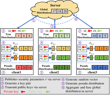
Figure 11. The example of PASS

Appendix G Security Analysis of PASS

PASS reveals little additional information with others beyond the pseudo-distribution and public key, which reduces the risk of privacy breaches. Next, we analyse the privacy protection ability of $PASS$ in the context of limited sharing of information.

Theorem G.1.

Any combination based on client-generated pseudo data distributions is computationally indistinguishable from a uniformly sampled element $\mathbb{Z}$ of the same space by the server, except for the aggregation combining all clients.

Proof.

For any $\{\mathbb{N}_{e}\}_{e\in\mathbb{E}}$, where $\forall e\in\mathbb{E}$, $\mathbb{N}_{e}\in\mathbb{R}^{C}$. If $e$ has the $\mathbb{RV}_{e,v}\in\mathbb{R}^{C},$ and $v$ has the corresponding $\mathbb{RV}_{v,e}=-\mathbb{RV}_{e,v}$. Then each client $e$ adds all $\mathbb{RV}_{e,v}$ with $\mathbb{N}_{e}$ gets:

(29) $$\mathbb{Y}=\{\mathbb{N}_{e}+\sum_{v\in\mathbb{E}\setminus\{e\}}\mathbb{RV}_{e,v}\}_{e\in\mathbb{E}}$$

Considering any combination from $\mathbb{Y}$, it can be defined as:

(30) $$\sum_{e\in\mathbb{I}\subseteq\mathbb{E}}\{\mathbb{N}_{e}+\sum_{v\in\mathbb{E}\setminus\{e\}}\mathbb{RV}_{e,v}\}$$

Then we compare it with a random generated element $\mathbb{Z}$ of the same space $\mathbb{Z}\in\mathbb{R}^{C}$. Then we can consider:

(31) $$\sum_{e\in\mathbb{I}\subseteq\mathbb{E}}\{\mathbb{N}_{e}+\sum_{v\in\mathbb{E}\setminus\{e\}}\mathbb{RV}_{e,v}\}\equiv\mathbb{Z}\qquad s.t.\quad\mathbb{I}\neq\mathbb{E}$$

When $\mathbb{I}\neq\mathbb{E}$, the sum of the client-generated pseudo distributions looks random. In other words, only when all the client-generated pseudo data distributions are aggregated, the server can obtain a non-random distribution, which is the global distribution we desire. ∎

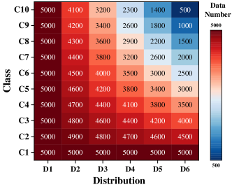
(a) Distribution List of CIFAR-10

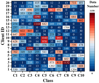
(b) Allocating CIFAR-10 D1 into Clients

Figure 12. The generated data distributions of CIFAR-10 and an example of its allocation

Theorem G.2.

The proposed mechanism can protect clients’ privacy in the semi-honest client environment.

Proof.

Each client $e$ generates a key pair $(SK_{e},PK_{e})$ and every client has its personalized key pair. Clients only transmit their public key $PK_{e}$ to other clients and the private key $SK_{e}$ don’t transmit in any form. Thus, $SK_{e}$ will not be eavesdropped by others.

The adversary client $a$ gets the public key of client $e$ and generates random seed $s_{a,e}$ which is the same as client $e$ generated. Then client $a$ generates $\mathbb{RV}_{a,e}\leftarrow\epsilon_{a,e}\cdot PRG(s_{a,e})$. According to the protocol client $a$ can infer $\mathbb{RV}_{e,a}=-\mathbb{RV}_{a,e}$ because $\epsilon_{a,e}=-\epsilon_{e,a}$. However, $\mathbb{RV}_{e,a}$ and $PK_{e}$ are all the information that client $a$ can get about the client $e$.

$\mathbb{N}_{e}$ can be inferred from Equation (32). It means only getting all the $\mathbb{RV}_{e,v}$ and $\mathbb{Y}_{e}$, the privacy of $e$ can be breached. The $\mathbb{RV}_{e,v}$ are generated locally on the clients and are not transmitted, so stealing them is very difficult.

(32) $$\small\mathbb{N}_{e}=\mathbb{Y}_{e}-\sum_{v\in\mathbb{E}\setminus{\{e\}}}\mathbb{RV}_{e,v}$$

As analysed above, client $a$ can only infer one $\mathbb{RV}_{e,v}$ about client $e$. Therefore, even if $a$ manages to obtain $\mathbb{Y}_{e}$ through certain means, it is still unable to compromise the privacy of $e$ due to lack of other $\mathbb{RV}_{e,v}$.

Therefore, our mechanism can protect the clients’ privacy in the semi-honest client environment. ∎

Theorem G.3.

The proposed mechanism can protect clients’ privacy in the semi-honest server environment.

Proof.

The server has access to the public key $PK_{e}$ but not to any of the private key $SK_{e}$ of each client $e$. The only value sent by each client $e$ is the pseudo distribution $\mathbb{Y}_{e}$. The server is unable to access the random seed $s_{e,v}$ since it is not shared by clients. In addition, the server can not generate it due to the lack of the necessary private keys, $SK_{e}$ or $SK_{v}$. Thus, $\mathbb{RV}_{e,v}\leftarrow\epsilon_{e,v}\cdot PRG(s_{e,v})$ as the key part to infer the privacy of client $e$ based on Equation (32) is difficult to obtain for the server.

As a result, only two messages the server can get. One is the pseudo distribution $\mathbb{Y}_{e}$ of clients and the other is the global distribution $\mathbb{N}_{s}$ combined with all pseudo distribution $\mathbb{Y}_{e}$. ∎

Appendix H The example of generating training dataset

Figure 12a demonstrates the process of transforming the originally balanced global data distribution (a total of 50K data, with 5K in each class) of the CIFAR-10 dataset into an unbalanced distribution. We incrementally remove data from each class to produce unbalanced global distributions, labeled as D2 to D6. In the second step, based on the different global data distributions, we allocate data for each class to each client following a Dirichlet distribution ($\alpha=0.5$) for simulating Non-i.i.d. scenarios (Hsu et al., 2019; Li et al., 2022; Lin et al., 2020). Figure 12b shows the results of distributing the D1 global distribution to 20 clients.

Appendix I Description of baselines

A brief description of the baselines used in our experiments is provided below:

• Random Selection (RS): a simple method that randomly selects a fixed number of clients.

• Quantity Based Selection (QBS) (Zeng et al., 2020): QBS selects a fixed number of clients only based on their data volumes in descending order.

• DICE (Saha et al., 2022): DICE selects clients with the highest data quality scores, defined in terms of the data volume ratio and the standard deviation of data volume in different categories.

• Diversity-driven Selection (DDS) (Li et al., 2021): DDS selects a subset of clients based on two criteria, (i) Statistical homogeneity, which assesses the similarity between a client’s distribution and a uniform distribution; ii) Content diversity, which measures the distance between clients on embedding vectors of their dataset. The selection process favours clients with both high statistical homogeneity and content diversity.

• S-FedAvg (Nagalapatti and Narayanam, 2021): an in-training client selection method where the Sharply value of local model accuracy is introduced after each round of training. In addition, a Shapley value-based Federated Averaging (S-FedAvg) algorithm is presented to select clients with high contributions to the FL task.

Appendix J communication analysis

Clients Side Analysis. On the client side, the communication cost consists of two parts: In the first part, each client uploads its public key to the server, which distributes it to other clients, then receives $(E-1)$ public keys of other clients from the server. The communication cost of the first part is $(1+(E-1))L_{k}=EL_{k}$, where $L_{k}$ is the number of bits in the public key exchange. In the second part, each client uploads its pseudo data distribution $\mathbb{Y}_{e}$ to the server, the size of $\mathbb{Y}_{e}$ is $C\lceil\log_{2}y_{e}^{c}\rceil$ ($y_{e}^{c}$ is the element of $\mathbb{Y}_{e}$ and $\lceil\log_{2}y_{e}^{c}\rceil$ is the minimum number of bits required for $y_{e}^{c}$). The communication cost is $C\lceil\log_{2}y_{e}^{c}\rceil$. Then the total communication cost of each client is $EL_{k}+C\lceil\log_{2}y_{e}^{c}\rceil$,

Server Side Analysis. On the server side, the two parts of communication cost are public key exchange and pseudo data distribution reception respectively. For the public key exchange part, the communication cost of public key reception is $EL_{k}$ and the dispatch communication cost is $(E(E-1))L_{k}$. The total communication cost of public key exchange is $E^{2}L_{k}$. For pseudo data distribution receptiotn, he communication cost is $EC\lceil\log_{2}y_{e}^{c}\rceil$.

Communication Cost of FL Training. In each round of FL training, clients upload the local model parameters to the server and receive the global model parameters from the server. The communication cost of each client is $2ML_{m}$, $M$ is the total number of model parameters and $L_{m}$ is the number of bits in each parameter. The communication cost of the server is $2ML_{m}E$ due to the server transmitting the model parameters for each client. This communication cost will happen in each round of FL training.

The number of parameters in the model is far greater than the class number and client number. Therefore the communication cost of FL training is far greater than PASS.

Appendix K Evaluation of FLMarket on the total number of 100 clients

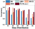
(a) 25 clients selected

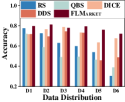
(b) 50 clients selected

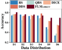
(c) 75 clients selected

Figure 13. CIFAR-10: $n$ clients selected from 100 clients

To evaluate the performance of FLMarket with a large number of clients, we present the results obtained from experiments in which 25, 50, and 75 clients were selected from a pool of 100 clients. The global data distributions remain consistent with those depicted in Figure 3, with the only difference being the number of clients. Figure 13 illustrates that FLMarket continues to achieve significant average accuracy improvements of 14.66 $\%$, 22.06 $\%$, 5.19 $\%$ and 11.08 $\%$ when compared to other baseline methods, with a large number of clients. However, comparing Figure 13 and 3, when the client pool is enlarged and more clients are selected, the accuracy improvement of FLMarket drops by 1-5 $\%$. This is because selecting more clients increases the probability of baseline methods to select high-quality clients.

References

- (1)
- Basu et al. (2021) Priyam Basu, Tiasa Singha Roy, Rakshit Naidu, and Zumrut Muftuoglu. 2021. Privacy enabled Financial Text Classification using Differential Privacy and Federated Learning. In Proceedings of the Third Workshop on Economics and Natural Language Processing. Association for Computational Linguistics, Punta Cana, Dominican Republic, 50–55. https://doi.org/10.18653/v1/2021.econlp-1.7
- Ben-David et al. (2010) Shai Ben-David, John Blitzer, Koby Crammer, Alex Kulesza, Fernando Pereira, and Jennifer Wortman Vaughan. 2010. A theory of learning from different domains. Machine learning 79 (2010), 151–175.
- Bonawitz et al. (2017) Keith Bonawitz, Vladimir Ivanov, Ben Kreuter, Antonio Marcedone, H Brendan McMahan, Sarvar Patel, Daniel Ramage, Aaron Segal, and Karn Seth. 2017. Practical secure aggregation for privacy-preserving machine learning. In proceedings of the 2017 ACM SIGSAC Conference on Computer and Communications Security. 1175–1191.
- Chen and Ohrimenko (2023) Michelle Chen and Olga Ohrimenko. 2023. Protecting global properties of datasets with distribution privacy mechanisms. In International Conference on Artificial Intelligence and Statistics. PMLR, 7472–7491.
- Darlow et al. (2018) Luke N Darlow, Elliot J Crowley, Antreas Antoniou, and Amos J Storkey. 2018. Cinic-10 is not imagenet or cifar-10. arXiv:1810.03505 (2018).
- Dayan et al. (2021) Ittai Dayan, Holger R Roth, Aoxiao Zhong, Ahmed Harouni, et al. 2021. Federated learning for predicting clinical outcomes in patients with COVID-19. Nature medicine 27, 10 (2021), 1735–1743.
- Deng et al. (2021a) Yongheng Deng, Feng Lyu, Ju Ren, Yi-Chao Chen, Peng Yang, Yuezhi Zhou, and Yaoxue Zhang. 2021a. Fair: Quality-aware federated learning with precise user incentive and model aggregation. In IEEE INFOCOM 2021-IEEE Conference on Computer Communications. IEEE, 1–10.
- Deng et al. (2022) Yongheng Deng, Feng Lyu, Ju Ren, Yi-Chao Chen, Peng Yang, Yuezhi Zhou, and Yaoxue Zhang. 2022. Improving federated learning with quality-aware user incentive and auto-weighted model aggregation. IEEE Transactions on Parallel and Distributed Systems 33, 12 (2022), 4515–4529.
- Deng et al. (2021b) Yongheng Deng, Feng Lyu, Ju Ren, Huaqing Wu, Yuezhi Zhou, Yaoxue Zhang, and Xuemin Shen. 2021b. Auction: Automated and quality-aware client selection framework for efficient federated learning. IEEE Transactions on Parallel and Distributed Systems 33, 8 (2021), 1996–2009.
- Deshpande and Karypis (2004) Mukund Deshpande and George Karypis. 2004. Item-based top-n recommendation algorithms. ACM Transactions on Information Systems (TOIS) 22, 1 (2004), 143–177.
- Gao et al. (2021) Liang Gao, Li Li, Yingwen Chen, Wenli Zheng, ChengZhong Xu, and Ming Xu. 2021. Fifl: A fair incentive mechanism for federated learning. In Proceedings of the 50th International Conference on Parallel Processing. 1–10.
- Hartmann et al. (2023) Valentin Hartmann, Léo Meynent, Maxime Peyrard, Dimitrios Dimitriadis, Shruti Tople, and Robert West. 2023. Distribution inference risks: Identifying and mitigating sources of leakage. In 2023 IEEE Conference on Secure and Trustworthy Machine Learning (SaTML). IEEE, 136–149.
- He et al. (2016) Kaiming He, Xiangyu Zhang, Shaoqing Ren, and Jian Sun. 2016. Deep residual learning for image recognition. In Proceedings of the IEEE conference on computer vision and pattern recognition. 770–778.
- Hellman (1976) Martin Hellman. 1976. New directions in cryptography. IEEE transactions on Information Theory 22, 6 (1976), 644–654.
- Hsu et al. (2019) Tzu-Ming Harry Hsu, Hang Qi, et al. 2019. Measuring the effects of non-identical data distribution for federated visual classification. arXiv:1909.06335 (2019).
- Hu et al. (2022) Miao Hu, Di Wu, Yipeng Zhou, Xu Chen, and Min Chen. 2022. Incentive-aware autonomous client participation in federated learning. IEEE Transactions on Parallel and Distributed Systems 33, 10 (2022), 2612–2627.
- Kaplan et al. (2020) Jared Kaplan, Sam McCandlish, Tom Henighan, Tom B Brown, Benjamin Chess, Rewon Child, Scott Gray, Alec Radford, Jeffrey Wu, and Dario Amodei. 2020. Scaling laws for neural language models. arXiv preprint arXiv:2001.08361 (2020).
- Koelstra et al. (2011) Sander Koelstra, Christian Muhl, Mohammad Soleymani, Jong-Seok Lee, Ashkan Yazdani, Touradj Ebrahimi, Thierry Pun, Anton Nijholt, and Ioannis Patras. 2011. Deap: A database for emotion analysis; using physiological signals. IEEE transactions on affective computing 3, 1 (2011), 18–31.
- Krizhevsky et al. (2009) Alex Krizhevsky, Geoffrey Hinton, et al. 2009. Learning multiple layers of features from tiny images. (2009).
- Lai et al. (2021) Fan Lai, Xiangfeng Zhu, Harsha V Madhyastha, and Mosharaf Chowdhury. 2021. Oort: Efficient federated learning via guided participant selection. In 15th USENIX Symposium on Operating Systems Design and Implementation (OSDI 21). 19–35.
- Li et al. (2021) Anran Li, Lan Zhang, Juntao Tan, Yaxuan Qin, Junhao Wang, and Xiang-Yang Li. 2021. Sample-level data selection for federated learning. In IEEE INFOCOM 2021-IEEE Conference on Computer Communications. IEEE, 1–10.
- Li et al. (2022) Qinbin Li, Yiqun Diao, Quan Chen, and Bingsheng He. 2022. Federated learning on non-iid data silos: An experimental study. In 2022 IEEE 38th International Conference on Data Engineering (ICDE). IEEE, 965–978.
- Li et al. (2023) Qi Li, Zhuotao Liu, Qi Li, and Ke Xu. 2023. martFL: Enabling Utility-Driven Data Marketplace with a Robust and Verifiable Federated Learning Architecture. In Proceedings of the 2023 ACM SIGSAC Conference on Computer and Communications Security. 1496–1510.
- Li et al. (2020) Tian Li, Anit Kumar Sahu, Manzil Zaheer, Maziar Sanjabi, Ameet Talwalkar, and Virginia Smith. 2020. Federated optimization in heterogeneous networks. Proceedings of Machine learning and systems 2 (2020), 429–450.
- Li et al. (2024) Zitao Li, Bolin Ding, Liuyi Yao, Yaliang Li, Xiaokui Xiao, and Jingren Zhou. 2024. Performance-Based Pricing for Federated Learning via Auction. Proceedings of the VLDB Endowment 17, 6 (2024), 1269–1282.
- Lin et al. (2019) Jierui Lin, Min Du, and Jian Liu. 2019. Free-riders in federated learning: Attacks and defenses. arXiv:1911.12560 (2019).
- Lin et al. (2020) Tao Lin, Lingjing Kong, Sebastian U Stich, and Martin Jaggi. 2020. Ensemble distillation for robust model fusion in federated learning. Advances in Neural Information Processing Systems 33 (2020), 2351–2363.
- Lin et al. (2021) Yaguang Lin, Zhipeng Cai, Xiaoming Wang, Fei Hao, Liang Wang, and Akshita Maradapu Vera Venkata Sai. 2021. Multi-round incentive mechanism for cold start-enabled mobile crowdsensing. IEEE Transactions on Vehicular Technology 70, 1 (2021), 993–1007.
- Liu et al. (2020) Yuan Liu, Zhengpeng Ai, Shuai Sun, Shuangfeng Zhang, Zelei Liu, and Han Yu. 2020. Fedcoin: A peer-to-peer payment system for federated learning. In Federated Learning. Springer, 125–138.
- Liu and Hacigümüs (2014) Ziyang Liu and Hakan Hacigümüs. 2014. Online optimization and fair costing for dynamic data sharing in a cloud data market. In Proceedings of the 2014 ACM SIGMOD International Conference on Management of Data. 1359–1370.
- Mao et al. (2024) Wuxing Mao, Qian Ma, Guocheng Liao, and Xu Chen. 2024. Game Analysis and Incentive Mechanism Design for Differentially Private Cross-silo Federated Learning. IEEE Transactions on Mobile Computing (2024).
- McAfee and McMillan (1987) R Preston McAfee and John McMillan. 1987. Auctions and bidding. Journal of economic literature 25, 2 (1987), 699–738.
- Nagalapatti and Narayanam (2021) Lokesh Nagalapatti and Ramasuri Narayanam. 2021. Game of gradients: Mitigating irrelevant clients in federated learning. In Proceedings of the AAAI Conference on Artificial Intelligence, Vol. 35. 9046–9054.
- Nishio and Yonetani (2019) Takayuki Nishio and Ryo Yonetani. 2019. Client selection for federated learning with heterogeneous resources in mobile edge. In ICC 2019-2019 IEEE international conference on communications (ICC). IEEE, 1–7.
- Perazzone et al. (2022) Jake Perazzone, Shiqiang Wang, Mingyue Ji, and Kevin S Chan. 2022. Communication-efficient device scheduling for federated learning using stochastic optimization. In IEEE INFOCOM 2022-IEEE Conference on Computer Communications. IEEE, 1449–1458.
- Qian et al. (2020) Bin Qian, Jie Su, Zhenyu Wen, Devki Nandan Jha, Yinhao Li, Yu Guan, Deepak Puthal, Philip James, Renyu Yang, Albert Y Zomaya, et al. 2020. Orchestrating the development lifecycle of machine learning-based IoT applications: A taxonomy and survey. ACM Computing Surveys (CSUR) 53, 4 (2020), 1–47.
- Ren et al. (2023) Kean Ren, Guocheng Liao, Qian Ma, and Xu Chen. 2023. Differentially Private Auction Design for Federated Learning with non-IID Data. IEEE Transactions on Services Computing (2023), 1–12.
- Ribero and Vikalo (2020) Monica Ribero and Haris Vikalo. 2020. Communication-efficient federated learning via optimal client sampling. arXiv:2007.15197 (2020).
- Saha et al. (2022) Rituparna Saha, Sudip Misra, Aishwariya Chakraborty, Chandranath Chatterjee, and Pallav Kumar Deb. 2022. Data-Centric Client Selection for Federated Learning Over Distributed Edge Networks. IEEE Transactions on Parallel and Distributed Systems 34, 2 (2022), 675–686.
- Schomm et al. (2013) Fabian Schomm, Florian Stahl, and Gottfried Vossen. 2013. Marketplaces for data: an initial survey. ACM SIGMOD Record 42, 1 (2013), 15–26.
- Singer (2010) Yaron Singer. 2010. Budget feasible mechanisms. In 2010 IEEE 51st Annual Symposium on foundations of computer science. IEEE, 765–774.
- Song et al. (2019) Tianshu Song et al. 2019. Profit allocation for federated learning. In 2019 IEEE International Conference on Big Data (Big Data). IEEE, 2577–2586.
- Spiekermann et al. (2015) Sarah Spiekermann, Alessandro Acquisti, Rainer Böhme, and Kai-Lung Hui. 2015. The challenges of personal data markets and privacy. Electronic markets 25 (2015), 161–167.
- Sun et al. (2022) Peng Sun, Xu Chen, Guocheng Liao, and Jianwei Huang. 2022. A profit-maximizing model marketplace with differentially private federated learning. In IEEE INFOCOM 2022-IEEE Conference on Computer Communications. IEEE, 1439–1448.
- Sun et al. (2024) Peng Sun, Guocheng Liao, Xu Chen, and Jianwei Huang. 2024. A Socially Optimal Data Marketplace With Differentially Private Federated Learning. IEEE/ACM Transactions on Networking (2024).
- Tang and Wong (2021) Ming Tang and Vincent WS Wong. 2021. An incentive mechanism for cross-silo federated learning: A public goods perspective. In IEEE INFOCOM 2021-IEEE Conference on Computer Communications. IEEE, 1–10.
- Wan et al. (2023) Xiaole Wan, Dongqian Yang, Tongtong Wang, and Muhammet Deveci. 2023. Closed-loop supply chain decision considering information reliability and security: should the supply chain adopt federated learning decision support systems? Annals of Operations Research (2023), 1–37.
- Wang et al. (2021a) Cong Wang, Yuanyuan Yang, and Pengzhan Zhou. 2021a. Towards Efficient Scheduling of Federated Mobile Devices Under Computational and Statistical Heterogeneity. IEEE Transactions on Parallel and Distributed Systems 32, 2 (2021), 394–410. https://doi.org/10.1109/TPDS.2020.3023905
- Wang et al. (2019) Guan Wang, Charlie Xiaoqian Dang, and Ziye Zhou. 2019. Measure contribution of participants in federated learning. In 2019 IEEE International Conference on Big Data (Big Data). IEEE, 2597–2604.
- Wang et al. (2020) Hongyi Wang, Mikhail Yurochkin, Yuekai Sun, Dimitris Papailiopoulos, and Yasaman Khazaeni. 2020. Federated learning with matched averaging. arXiv preprint arXiv:2002.06440 (2020).
- Wang et al. (2024) Jianhua Wang, Xiaolin Chang, Jelena Mišić, Vojislav B. Mišić, and Yixiang Wang. 2024. PASS: A Parameter Audit-Based Secure and Fair Federated Learning Scheme Against Free-Rider Attack. IEEE Internet of Things Journal 11, 1 (2024), 1374–1384.
- Wang et al. (2022) Junxiao Wang, Song Guo, Xin Xie, and Heng Qi. 2022. Protect privacy from gradient leakage attack in federated learning. In IEEE INFOCOM 2022-IEEE Conference on Computer Communications. IEEE, 580–589.
- Wang et al. (2021b) Qinyong Wang, Hongzhi Yin, Tong Chen, Junliang Yu, Alexander Zhou, and Xiangliang Zhang. 2021b. Fast-adapting and privacy-preserving federated recommender system. The VLDB Journal 31, 5 (oct 2021), 877–896.
- Xu et al. (2021) Xinyi Xu, Lingjuan Lyu, Xingjun Ma, Chenglin Miao, Chuan Sheng Foo, and Bryan Kian Hsiang Low. 2021. Gradient driven rewards to guarantee fairness in collaborative machine learning. Advances in Neural Information Processing Systems 34 (2021), 16104–16117.
- Yao (1982) Andrew C Yao. 1982. Theory and application of trapdoor functions. In 23rd Annual Symposium on Foundations of Computer Science (SFCS 1982). IEEE, 80–91.
- Zeng et al. (2022) Rongfei Zeng, Chao Zeng, Xingwei Wang, Bo Li, and Xiaowen Chu. 2022. Incentive Mechanisms in Federated Learning and A Game-Theoretical Approach. IEEE Network 36, 6 (2022), 229–235.
- Zeng et al. (2020) Rongfei Zeng, Shixun Zhang, Jiaqi Wang, and Xiaowen Chu. 2020. Fmore: An incentive scheme of multi-dimensional auction for federated learning in mec. In 2020 IEEE 40th International Conference on Distributed Computing Systems (ICDCS). IEEE, 278–288.
- Zhan et al. (2020) Yufeng Zhan, Peng Li, Zhihao Qu, Deze Zeng, and Song Guo. 2020. A learning-based incentive mechanism for federated learning. IEEE Internet of Things Journal 7, 7 (2020), 6360–6368.
- Zhan et al. (2021) Yufeng Zhan, Jie Zhang, Zicong Hong, Leijie Wu, Peng Li, and Song Guo. 2021. A survey of incentive mechanism design for federated learning. IEEE Transactions on Emerging Topics in Computing 10, 2 (2021), 1035–1044.
- Zhang et al. (2021b) Jingwen Zhang, Yuezhou Wu, and Rong Pan. 2021b. Incentive mechanism for horizontal federated learning based on reputation and reverse auction. In Proceedings of the Web Conference 2021. 947–956.
- Zhang et al. (2021a) Wanrong Zhang, Shruti Tople, and Olga Ohrimenko. 2021a. Leakage of dataset properties in Multi-Party machine learning. In 30th USENIX security symposium (USENIX Security 21). 2687–2704.
- Zheng et al. (2022) Shuyuan Zheng, Yang Cao, Masatoshi Yoshikawa, Huizhong Li, and Qiang Yan. 2022. FL-Market: Trading private models in federated learning. In 2022 IEEE International Conference on Big Data (Big Data). IEEE, 1525–1534.
- Zheng et al. (2016) Zhenzhe Zheng, Fan Wu, Xiaofeng Gao, Hongzi Zhu, Shaojie Tang, and Guihai Chen. 2016. A budget feasible incentive mechanism for weighted coverage maximization in mobile crowdsensing. IEEE Transactions on Mobile Computing 16, 9 (2016), 2392–2407.
- Zhou et al. (2021) Ruiting Zhou, Jinlong Pang, Zhibo Wang, John CS Lui, and Zongpeng Li. 2021. A truthful procurement auction for incentivizing heterogeneous clients in federated learning. In 2021 IEEE 41st International Conference on Distributed Computing Systems (ICDCS). IEEE, 183–193.