Hamiltonian Monte Carlo vs. event-chain Monte Carlo:
an appraisal of sampling strategies beyond the diffusive regime
Abstract
We discuss Hamiltonian Monte Carlo (HMC) and event-chain Monte Carlo (ECMC) for the one-dimensional chain of particles with harmonic interactions and benchmark them against local reversible Metropolis algorithms. While HMC achieves considerable speedup with respect to local reversible Monte Carlo algorithms, its autocorrelation functions of global observables such as the structure factor have slower scaling with system size than for ECMC, a lifted non-reversible Markov chain. This can be traced to the dependence of ECMC on a parameter of the harmonic energy, the equilibrium distance, which drops out when energy differences or gradients are evaluated. We review the recent literature and provide pseudocodes and Python programs. We finally discuss related models and generalizations beyond one-dimensional particle systems.
1 Introduction
Markov-chain Monte Carlo (MCMC) permeates all fields of science, from physics to statistics and to the social disciplines. Reversible Markov chains, the great majority of MCMC methods, map the sampling of probability distributions onto the simulation of fictitious physical systems in thermal equilibrium. In physics, thermal equilibrium is characterized by time-reversal invariance and the detailed-balance condition. It thus comes as no surprise that reversible Markov chains, such as the famous Metropolis [1] and heat-bath algorithms [2, 3, 4], all satisfy detailed balance. In physics, again, thermal equilibrium is characterized by diffusive, local, motion of particles. This translates into the slow mixing and relaxation dynamics of local reversible Markov chains, and it affects most Markov chains used in practice.
In this paper, we appraise diametrically opposite strategies to overcome the slow diffusive motion of local, reversible MCMC methods. One is Hamiltonian Monte Carlo (HMC), a non-local yet reversible Markov chain, and the other is event-chain Monte Carlo (ECMC), a class of lifted Markov chains, which are local yet non-reversible.
HMC [5] emulates classical physical systems which, even when they are out of equilibrium, satisfy Newton’s (or Hamilton’s) equations. In addition to their positions (the sample-space variables of the fictitious physical systems), particle systems have momenta. While the positions change in time as dictated by the momenta, momenta change with the gradient of a potential. Approaching equilibrium then corresponds to a gradient descent, which is generally assumed to be fast because it corresponds to a physical dynamics. In a nutshell, HMC introduces fictitious momenta and solves discretized Newton’s equation to move from one configuration to a distant configuration . The time-discretization errors are eliminated through rejections which enforce detailed balance.
ECMC [6, 7] introduces additional “lifting” variables which are more general than momenta. As the name indicates, ECMC is an event-driven implementation of a continuous-time (thus local) Markov process. It thus need not discretize time, and exactly satisfies global balance, a continuity condition which replaces detailed balance in the non-reversible case. The ECMC dynamics is neither diffusive nor gradient-based. In fact, it evaluates no global potential, potential differences or gradients, and it crucially depends on a parameter (a “factor field” [8] or “pullback” [9]), which leaves the gradient invariant. For a many-particle harmonic chain on a one-dimensional ring that we use as a benchmark, ECMC has better scaling than HMC.
In Section 2 of this paper, we review the harmonic chain [8], compute its thermodynamics, and present basic sampling algorithms for it, on the one hand direct-sampling methods, and on the other the aforementioned local reversible Markov chains featuring slow diffusive dynamics. In Section 3, we implement an HMC algorithm for the harmonic chain, following Ref. [10], and discuss the algorithm’s stability and its relation to the molecular-dynamics method. In Section 4, we implement several variants of ECMC for the harmonic chain, following Ref. [8]. We discuss the essential link [7] between the behavior of the algorithm and the system pressure and outline how the algorithm has been generalized to more complex sampling problems. In Section 5, we juxtapose the different sampling strategies and show how they effectively go beyond the diffusive regime and improve the scaling of autocorrelation times of global observables, in our case the structure factor. In the concluding Section 6 we discuss the generic nature of the harmonic-chain dynamics both for HMC and ECMC. We also discuss the relation of ECMC for the harmonic chain with a lattice model, the “lifted” TASEP (totally asymmetric simple exclusion model), whose dynamics can be analyzed exactly using the Bethe ansatz [9]. The main text of this paper contains a number of pseudocode algorithms. The appendices provide mathematical details (Appendix A), as well as further pseudocode algorithms and pointers towards an open-source repository containing all the Python programs discussed in this paper (Appendix B).
2 Harmonic chain: thermodynamics and basic sampling
The harmonic chain describes particles on a continuous interval with periodic boundary conditions in space and in the indices. Each particle interacts with the two particles with neighboring indices. The interaction is harmonic with an equilibrium pair distance that drops out for the Metropolis algorithm and for HMC but is all important within ECMC. The harmonic chain is equivalent to the time-discretized path integral of a free quantum particle [11].
In Section 2.1, we define the harmonic-chain model and exactly compute its thermodynamics, in particular the pressure, whose vanishing defines a special point for ECMC. We further discuss, in Section 2.2, direct-sampling algorithms for the harmonic chain and, in Section 2.3, examples of local reversible Markov chains featuring the slow dynamics that HMC and ECMC overcome in different ways. The Metropolis algorithm is the classic sampling approach, whereas the factorized Metropolis algorithm is the starting point for the nonreversible ECMC.
2.1 Model definition, thermodynamics
The harmonic chain consists of particles on a ring of length with periodic boundary conditions. For finite , a convenient description is in terms of one periodic coordinate
| (1) | |||
| and of elongations with | |||
| (2) | |||
| Periodic boundary conditions are implemented through | |||
| (3) | |||
Each configuration (with from eq. (3) understood) has a harmonic potential
| (4) | ||||
| (5) | ||||
| (6) |
with the equilibrium pair distance . In eq. (6), the terms in are the same for all particle positions, so that algorithms that rely on potential differences and gradients, such as HMC, are insensitive to them. They play nevertheless a crucial role for ECMC dynamics [8].
The Boltzmann weight of each configuration is given by
| (7) |
with the partition function
| (8) | ||||
| (9) |
(see Appendix A for a derivation). The pressure is
| (10) |
For , the pressure vanishes. This defines a special point for ECMC. The mean energy is
| (11) |
Its -independent part (the last two terms on the right-hand side) will be used for testing our computer implementations.
The gradient of the energy,
| (12) |
is independent of . The harmonic chain is defined in terms of distinguishable particles, which allows to define elongations between ). Throughout this paper, we only consider observables which are invariant under a uniform translation of the positions. This has been formalized as a difference between a “configuration” and a “state” of a Markov chain [12].
2.2 Direct sampling: Lévy construction (Gaussian bridge)
The Boltzmann distribution of eq. (7) can be sampled directly, without resorting to Markov chains. One direct-sampling algorithm, the Lévy construction [13] (also known as the “Gaussian bridge”), is a staple in fields from path-integral Monte Carlo [14, 15] to financial mathematics [16]. The position is sampled as a uniform random variables between and . Then, as is known through eq. (3), one can iteratively sample a Gaussian (conditioned on and ) then another Gaussian (conditioned on and ) and so on until (see Alg. 1 (levy-harmonic)). The algorithm exists in many variants, including in Fourier space [11, Chap. 3]. All these algorithms are naturally independent of the equilibrium pair distance , reinforcing the naive conception that is irrelevant for sampling. We use the Lévy construction to initialize our Markov chains in equilibrium.
2.3 Metropolis and factorized Metropolis algorithms
Any Markov chain that is irreducible and aperiodic converges to the distribution if it satisfies the global-balance condition [17]
| (13) |
Here, the transition matrix is the probability to move from a given point to in one time step, from time to , conditioned on the Markov chain being at position at time . A stricter condition for convergence is the detailed-balance condition
| (14) |
which implies eq. (13) because of the conservation of probabilities . Commonly, the transition matrix is written as a product
| (15) |
Here, the a priori probability proposes the move , and the filter accepts or rejects it. The Metropolis algorithm uses a symmetric ,
| (16) |
with a specific choice of symmetric function:
| (17) |
As the right-hand side of this equation is symmetric in and , so must be the rest of the equation, so that detailed balance is satisfied. This leads to the famous Metropolis filter
| (18) |
In the harmonic chain, for a move of a single particle , the change of the potential , written as in eq. (4), impacts two terms, namely
| (19) | ||||
| in the initial configuration containing and two terms, namely | ||||
| (20) | ||||
for the final configuration containing (up to boundary conditions in space and in particle index, and ). Writing (and for the potentials of the new position), the Metropolis filter becomes
| (21) | ||||
| (22) |
This is implemented for in Alg. 2 (metropolis-harmonic), together with a consistent treatment of periodic boundary conditions in position and particle index. The algorithm is independent of , because of eqs. (4) and (6).
The factorized Metropolis algorithm [7] inherits the symmetric a priori probability from Alg. 2 (metropolis-harmonic), but uses a filter which is the product of two factor filters
| (23) | ||||
| (24) |
This filter may of course be implemented by comparing a random number to , but its true potential stems from rather comparing two independent random numbers to two factor filters, namely to and to . The move is accepted by consensus (see Ref. [18] for a discussion and Alg. 3 (metropolis-factorized-harmonic)). The explicit dependence will later allow the non-reversible ECMC to improve the scaling of relaxation times. Run reversibly, as in Alg. 3, it does not have this advantage. In fact, the factorized variant is slower than the traditional Metropolis algorithm simply because . It thus requires somewhat smaller values of than Alg. 2 in order to keep up a sizeable acceptance rate.
The dynamics of the factorized Metropolis algorithm explicitly depends on the choice of factors. As a simple alternative factorization, we may write the energy as in eq. (5) with four terms that change with a move of particle :
| (25) | ||||||
| (26) |
which then gives rise to four factor filters (see Alg. 8 (metropolis-fourfactor-harmonic) in Appendix B for an implementation). The term is referred to as a “factor field” [8]. It is related to the “pullback” of the lifted TASEP [9] and its generalizations [19], and can be set up for general potentials .
3 Hamiltonian Monte Carlo for the harmonic chain
“Hamiltonian” Monte Carlo [5] (originally termed “hybrid” Monte Carlo) implements a reversible Markov chain with a symmetric proposal probability, just as the Metropolis algorithm. It proposes large moves , but ensures that the acceptance probability remains high and thus improves on the reversible Markov chains of Alg. 2 and Alg. 3. However, computing given is is time-consuming, and the computational complexity for proposing the move is determined by an instability which becomes more pronounced for bigger sizes.
In Section 3.1, we implement HMC for the harmonic chain and sketch some of its basic properties. In Section 3.2, we discuss the optimal choice of parameters in order to propose and accept non-local moves most efficiently. In Section 3.3, we compare HMC to the molecular-dynamics method.
3.1 Implementation of HMC
HMC associates the position at a given time with a set of Gaussian momenta . Together, they construct a probability distribution
| (27) |
The energy thus becomes the potential energy of a dynamical system with total energy , where the kinetic energy is . An ideal Hamiltonian time evolution moves in a time interval from to . In the special case of the hard-sphere model, this dynamics samples the Boltzmann distribution rigorously [20, 21]. In more general problems, the (ideal) Hamiltonian time evolution conserves the total energy but may not visit all configurations of energy . In addition, the potential energy satisfies . With fixed, is also bounded. It is thus evident that the momenta must be resampled from eq. (27). In the aforementioned hard-sphere models and variants, ideal Hamiltonian time evolution can be implemented on the computer. This is the field of event-driven molecular dynamics [22, 23], which applies to models with piecewise constant potentials. In the general case, however, the evolution equations must be time-stepped, with a time-discretization interval . Symplectic time-stepping algorithms do generally not conserve the energy , so that the move generates an energy . However, the algorithms used in HMC are time-reversal invariant, and the Metropolis filter establishes detailed balance with respect to the true Boltzmann distribution, without any approximation or time-stepping error. The configuration equals if the move is accepted, and remains at otherwise. Algorithm 4 (hmc-harmonic) translates the example program of Ref. [10] into our context.
3.2 HMC acceptance rate, stability
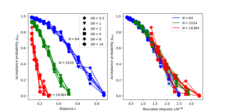
Much research has gone into the study of time-stepped dynamical systems [24] and the discretization errors introduced by finite values of . The key concept is that, with a finite , the discretized time evolution conserves the energy not of the hamiltonian with energy , but of a nearby “shadow” hamiltonian characterized by a potential energy . As , and is conserved, the energy (as a function of the index in Alg. 4) remains close to , allowing HMC to propose very large moves. The shadow hamiltonian usually describes the dynamics up to large timescales, but it hypothetical. Asymptotically, at very large times , the discretized dynamics gives rise to a drift [25]. However, for quadratic hamiltonians as the harmonic chain, the shadow hamiltonian actually exists [10, 26, 27]. As a consequence, the acceptance probability of the Metropolis filter in Alg. 4 (hmc-harmonic) is largely independent of for given , allowing for non-local moves whereas it vanishes exponentially with for Alg. 2 (metropolis-harmonic), keeping the moves local. This essential advantage of HMC is illustrated in Fig. 1. It survives up to very long times for general hamiltonians.
For fixed , the HMC algorithm reaches large moves, but the acceptance probability degrades with increasing stepsize, and it is essentially zero for large . For large , this problem becomes more pronounced. For a scaling , a universal acceptance probability is reached (see Fig. 1). This behavior is well understood theoretically [10].
3.3 Relation of HMC to molecular dynamics
HMC, as implemented in Alg. 4 (hmc-harmonic), contains three essential ingredients that are associated with distinct computations. The first ingredient is the repeated evaluation of the gradient which iteratively time-steps the leapfrog algorithm from (and its associated momentum ) to (and ). In the harmonic chain, this step is insensitive to the parameter , and its computational cost is operations per time step (that is, per iteration in Alg. 4). With long-range interactions, the evaluation of the gradient typically relies on fast Ewald methods [28] or multipole expansions [29] and cannot be performed efficiently to machine precision [30]. The second ingredient is the Metropolis filter that enforces the correct stationary distribution. It renders HMC reversible and rigorous. It evaluates the total-energy change between and , and is again independent of . In the general case, ECMC avoids the evaluation of or its derivatives yet still samples (see Ref. [31] for an introduction). The third ingredient is the refreshment (or thermalization) of the momenta—on the same time frame as the Metropolis step, which assures the irreducibility of the Markov chain. ECMC, as we will discuss later, also features auxiliary variables that are updated as the simulation proceeds, but never refreshed.
With its rejection step, HMC samples the stationary distribution exactly. It is thus a rigorous variant of molecular dynamics, the hamiltonian time evolution coupled to a thermostat at all time steps , but without a Metropolis decision. Such a thermostat hides instabilities (as shown in Fig. 1), accumulated errors and energy drifts. Thermostats thus may produce artifacts, but they often appear as a “necessary evils” [32]. ECMC evaluates neither gradients not differences of the total energy and requires no refreshments and no thermostats. Its dynamics, however, claims no similarity with the physical dynamics.
4 Event-chain Monte Carlo for the harmonic chain
For the harmonic chain, ECMC [6, 7] corresponds to the factorized Metropolis algorithm of Alg. 3 (or its variants) with three changes. First, only forward moves are proposed. This is feasible because of the periodic boundary conditions, but can be easily generalized. The a priori probability of eq. (16) is thus non-symmetric. Second, moves are infinitesimal, resulting in a continuous-time Markov process. The rejection probability is so small (it is infinitesimal), that most moves are accepted. Any rejection can be traced to a specific factor, and in Alg. 3 either to the forward factor (the one involving ) or to the backward factor (the one involving ), but not to both. Third, rejections are replaced by “liftings”. This means that, after an accepted (infinitesimal) move of particle , the same particle moves again. Otherwise, if ’s move is rejected by , will move next. If ’s move is rejected by , it is that will move next. The algorithm thus differs from the reversible local algorithms (Alg. 2 and Alg. 3) in that the particle to be moved at time is computed from the outcome of the simulation at time . The particle index is part of an enlarged “lifted” sample space. Lifted Markov chains [33, 34] build the conceptual underpinning of ECMC, a topic developed elsewhere [35].
In Section 4.1, we implement ECMC for the harmonic chain, as was already done in Ref. [8], starting from the factorized filter of eq. (24) for infinitesimal proposed moves . We then focus on the role of the pressure of this algorithm. In Section 4.2, we discuss other factorizations, in particular writing the energy as (that is, following eq. (5) rather than eq. (4)), which then allows for generalizations to arbitrary interactions. Finally, in Section 4.3, we discuss general properties of ECMC for the harmonic chain and its generalizations.
4.1 Implementation of ECMC, role of pressure
For the harmonic chain, ECMC may be implemented with the decomposition of eq. (4). An infinitesimal forward move of particle may change two terms in the above sum, giving rise to two independent factor filters:
| (28) | |||
For the eponymous event-driven implementation of ECMC, the time-and-space interval is not discretized [36]. This is possible because, after an accepted move of particle , the same particle moves again. For both factors, “downhill” moves are always accepted and “uphill” moves are accepted until the total energy change equals the logarithm of a uniform random number (see Ref. [18] for an introduction). For each factor, we thus accept the downhill motion (to positions in Alg. 5), then compute “candidate” events [37, 38], for each of the factors, and finally terminate the uphill move at the earliest of the candidate events, as it breaks the consensus at the heart of the factorized Metropolis filter. After the event with the active particle , the particle becomes active if the event involves , and the particle if it involves .
Alg. 5 (ecmc-harmonic) implements ECMC, moving forward from one event to the next. In practice, the algorithm may be stopped at regular time intervals, say, after a time (see the Python implementation of Alg. 5). At any generic time , the “pointer” (the position of the active particle ) moves forward with , but at an event, it jumps to the position or . These jumps can be in both directions. In a time , the pointer moves on average by a distance . The mean pointer speed is linearly related to the system pressure [7]:
| (29) |
It follows from eq. (10) that
| (30) |
with the global density and with as defined earlier (see Table 1). We may interpret this equation in two ways. First, for fixed global density , the pointer velocity is obviously a linear function of , hitting zero at . Second, for fixed at (neglecting the terms), local coarse-grained densities will lead to a (signed) local pointer velocity [39]:
| (31) |
In regions with an excess density, the pointer thus moves forward, and in regions with a density deficit, it moves backwards, getting trapped between any two such regions [39].
4.2 Facter-field ECMC interpretation
The factorization used in Alg. 5 (ecmc-harmonic) is by no means unique. An alternative is suggested by the decomposition (see eq. (5)), already implemented within the local reversible factorized Metropolis algorithm (see Alg. 8). The linear term in this decomposition, introduced in Ref. [8] as a “factor field”, sums up to zero because of the periodic boundary conditions, and can be added to any continuous potential. In the implementation of Alg. 6 (ecmc-fourfactor-harmonic), a move of a single particle changes four factors, and (naively) calls for the consensus of four decisions, of which one is to systematically accept the move. Remarkably, the mean pointer velocity of Alg. 6 is the same as that of Alg. 5.
4.3 Generalization of ECMC
ECMC implements a non-reversible Markov chain in the lifted sample space composed of the particle configuration and the identity of the active particle. For all values of the equilibrium pair distance it is irreducible and aperiodic. With its constant velocity (in this simplest setting), it does not conserve the energy , and the event-driven formulation sidesteps all the issues related to the discretization of time-driven dynamics. Finally, there are no thermostats. The ECMC algorithms studied here have been generalized in different directions. Newtonian ECMC, for example, ascribes velocities to all particles, but actually moves only a subset of them [40]. This then parallels the dynamics of the HMC, but it remains event-driven and non-reversible at all times and exactly samples the distribution . Variants of ECMC may [6] or may not [41] require refreshments [42]. ECMC is embedded in the framework of piecewise deterministic Markov processes [43, 44, 45].
5 Comparison of MCMC algorithms for the harmonic chain
In Section 2.1, we analytically obtained the thermodynamics of the harmonic string, in other words its steady-state behavior towards which all discussed algorithms converge rigorously. The complete independence of results on the step size and the number of iterations (for HMC) and on the equilibrium distance (for ECMC) is checked explicitly in Section 5.1, testing our implementations. HMC depends on two external parameters, namely the number of iterations and the stepsize , while ECMC depends on the equilibrium pair distance . Following Ref. [10] for HMC and Ref. [8] for ECMC, we discuss in Section 5.2 how to choose optimal parameters. Finally, in Section 5.3, we discuss the scaling of autocorrelation times with system size.
5.1 Mean energy
As a first check of our algorithms, we determine the -independent part of the mean energy . Five-digit precisions are obtained easily, and the agreement with the analytical result of eq. (11) is complete. All the MCMC computations start from an equilibrium configuration obtained by the Lévy construction, so that no error is introduced by the approach of the steady state (see Table 2). The absence of discretization errors is particularly remarkable. HMC, as discussed, propagates a shadow hamiltonian rather than the one corresponding to the energy . It is the Metropolis rejection step that enforces detailed balance with respect to the correct Boltzmann distribution. In ECMC, all rejections are, so to speak, re-branded into lifting moves, in our case the transfer of the pointer from one particle to another. Its event-driven setup, by definition, avoids all time-discretization. All Python programs are openly available (see Appendix B.2).
| Method | (-independent part) | see |
|---|---|---|
| exact | eq. (11) | |
| Lévy construction | Alg. 1 (levy-harmonic) | |
| Metropolis | Alg. 2 (metropolis-harmonic) | |
| Factorized () | Alg. 3 (metropolis-factorized-harmonic) | |
| Factor-field () | Alg. 8 (metropolis-fourfactor-harmonic) | |
| HMC () | Alg. 4 (hmc-harmonic) | |
| HMC () | Alg. 4 (hmc-harmonic) | |
| ECMC () | Alg. 5 (ecmc-harmonic) | |
| ECMC () | Alg. 5 (ecmc-harmonic) |
5.2 Parameter dependence of HMC and ECMC
For a configuration at time , we define the structure factor as:
| (32) |
where is the smallest non-zero wave number in a periodic system of length . The structure factor is sensitive to long-range density fluctuations, which are expected to relax slowly in equilibrium. It is invariant under uniform translations of all particles, and it does not require to know particle indices or the connectivity matrix. As in earlier works, we use the autocorrelation time of the structure factor to benchmark MCMC algorithms, but a number of related observables give equivalent results.
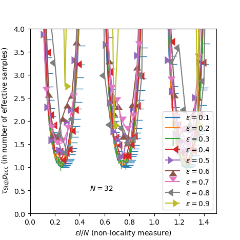
As discussed, HMC proposes non-local moves from the Newtonian evolution of an associated dynamical system. In the harmonic chain, these proposals are more efficient than those of the local Metropolis algorithm as, for , essentially a single long move decorrelates the Markov chain. The length of this chain requires fine-tuning to values in order to avoid recurrence with (see Fig. 2). For small non-zero step sizes , the quality of the proposed moves degrades gracefully, and it remains true that a single long, accepted, move decorrelates the Markov chain. The computing effort for one such move is , as we have to choose to keep the rejection rate under control.
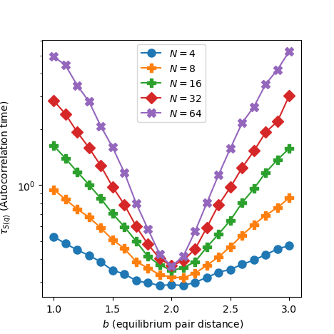
The performance of ECMC naturally depends on the equilibrium pair distance (in more general terms, on the factor field). The remarkable speedup of autorcorrelation times at , shown previously [8] in the harmonic chain and its generalizations, is shown again in Fig. 2.
5.3 Scaling of autocorrelation times
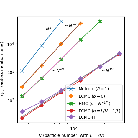
We again consider the harmonic chain of particles with , initialized in equilibrium through a direct sample of Alg. 1 (levy-harmonic). The data indicate that a local reversible Markov chain, here Alg. 2 (metropolis-harmonic), relaxes in single moves (see Fig. 3). This corresponds to “sweeps” of particles, in other words a dynamical scaling with exponent . This scaling is characteristic of models in the Edwards–Wilkinson class [46]. Relaxation in single steps is proven [47] rigorously for the symmetric simple exclusion model (SSEP), a discrete lattice reduction of the harmonic chain. The ECMC algorithm, for an unadjusted equilibrium pair distance , features a relaxation in single moves (or sweeps). This behavior was identified, in a related lattice model [48], as representing the universality class of the TASEP described by the Kardar–Parisi–Zhang (KPZ) exponent . For unadjusted pullback , the lifted TASEP likewise has an inverse gap [9]. HMC (with a stepsize ) and a chain length is very well compatible with the expected scaling behavior. Finally, the scaling of the autocorrelation time at confirms analogous prior computations in the same model [8]. The decay of autocorrelations was also found in the lifted TASEP [9]. The behavior is generic, and not related to the integrability of the Gaussian model and the lifted TASEP. Nevertheless, there is very strong evidence, from the Bethe ansatz, of an inverse gap scaling as in that model.
6 Discussion, conclusion
Reversible, local Markov chains form the backbone of the huge field of Monte Carlo methods. The reversibility of these methods brings in the detailed-balance condition, with which a move can be accepted or rejected using a filter involving only and . As we have discussed, the locality of these methods is the price to be paid for the move being generated blindly, in our case by a random displacement of a particle. Large moves exit the region of sample space with high weight (low energy), and get rejected. Local-move reversible MCMC algorithms for one-dimensional particle models generally have a diffusive relaxation time , and this can often be proven rigorously.
To propose non-local moves , HMC relies on “[g]eometric integrators [that] are time-stepping methods, designed so that they exactly satisfy conservation laws, symmetries, or symplectic properties of a system of differential equations” (quote from Ref. [24]). This results in custom-tailored, non-local moves, but which are costly to construct. In the harmonic chain, the leapfrog integrator of Newton’s equations comes with a time complexity , of which control the numerical instability of the geometric integrator, and moves each of the particles ballistically by a distance on the order of the system size. The time complexity (corresponding to sweeps) is only slightly larger than the dynamical scaling exponent associated with molecular dynamics. It is generic for a wide range of one-dimensional particle models, geometric integrators and differential equations.
To propose moves , ECMC relies on a class of event-stepping methods designed to exactly satisfy the very global-balance condition that encodes the stationarity of the Boltzmann distribution. The method has no rejections because, when a particle displacement is impossible, a “lifting” move takes place. Past research has shown this paradigm to adapt itself to real-life models in statistical mechanics [49] and chemical physics [30], with demonstrated speedups of several orders of magnitude [49, 50]. The harmonic chain demonstrates in a rather complicated setting that non-physical local dynamics can decorrelate even faster than the hamiltonian dynamics of HMC. This point was made for molecular dynamics rather than HMC, in Ref. [8].
What we have discussed here is in no way related to any special feature of the harmonic model. The scaling of autocorrelation functions at the critical factor field was observed also for Lennard-Jones interactions, and for hard spheres in the continuum. Furthermore, it is also a definite feature of the lifted TASEP [9], where the Bethe ansatz yields direct access to the excitation spectrum of the transition matrix. In both the harmonic chain and the lifted TASEP, the superior performance requires fine-tuning to vanishing pressure. However, this is easy, as the zero-pressure point corresponds to driftless pointer motion. In the lifted TASEP, there is compelling evidence for the existence, in any momentum sector, of a possibly isolated eigenvalue with an inverse-gap scaling [9]. The corresponding state seems not to couple to “normal” observables [19]. It is unknown whether such a state is present in the harmonic chain. The scaling at has natural support from a hydrodynamic viewpoint [39].
To make further progress, it appears important to study a possible synthesis between HMC and ECMC, for example whether modifications of the former can reach the scaling in the harmonic chain. In one-dimensional particle systems, it appears possible to fully understand the remarkable ECMC dynamics. The recently discovered deep connection between ECMC and the fully self-avoiding random walk[51, 52] merits full attention. Factor-field ECMC has also been implemented in higher-dimensional particle systems, where it relaxes density modes with great efficiency [53]. In more than one dimensions, the dynamics of non-reversible Markov chains needs to be much better characterized, and the recent focus on one-dimensional systems should be seen as a first step.
Acknowledgments
It is a pleasure to thank Nawaf Bou-Rabee, Bob Carpenter, Fabian Essler, and A. C. Maggs for inspiring discussions, and the Simons Center (Flatiron Institute) for hospitality. This research was supported by a grant from the Simons Foundation (Grant 839534, MET).
Appendix A Mathematical details
We compute the partition function of the harmonic chain, retaining the dependence on in order to compute the internal energy. The partition function of the model defined by eq. (4) to eq. (6) is
| (33) | ||||
| (34) |
with understood. In eq. (34), the exponential contains terms with . We may change the boundary conditions to eliminate through the transformation:
| (35) | ||||
| (36) |
resulting in:
| (37) | ||||
| (38) |
Here, the prefactor comes from the integration of , which we now fix to . The coefficient can be absorbed in a rescaling of the , so that the integral in eq. (38) becomes
| (39) |
with an Toeplitz matrix (setting )
| (40) |
leading to eq. (9). For the logarithm of the partition function, we have
| (41) |
which implies eqs. (10) and (11) for the pressure and the mean energy.
Appendix B Sampling algorithms, implementations, website
For the sake of completeness, we present two more sampling algorithms, one being a local Gibbs sampler, and the other the local reversible four-factor Metropolis algorithm, which serves as a starting point for the factor-field variant of ECMC (Alg. 6 (ecmc-fourfactor-harmonic)).
B.1 Additional pseudocode algorithms
In a heat-bath algorithm (Gibbs sampler), a subsystem of the configuration is equilibrated with respect to its environment. The harmonic chain allows this subsystem to be the position of a single particle or any number of neigboring particles. This subsystem can be equilibrated through a variant of the Lévy construction, so that the Markov chain (implemented in Alg. 7 (gibbs-harmonic)) need not be local. This contrasts with the situation for the local Metropolis algorithm, where the step-size and the number of displaced particles must be small in order to keep a sizeable acceptance rate. In general models, the heat-bath and Metropolis algorithms behave similarly.
We provide the factorized Metropolis algorithm for the decomposition of the potential into the factors indicated by eqs. (25) and (26). The implementation is naive, and the decision can be reduced from the consensus of four factors to that of three factors (see Alg. 8 (metropolis-fourfactor-harmonic)). The algorithm is closely related to the alternative “factor-field” ECMC method Alg. 6 (ecmc-fourfactor-harmonic).
B.2 Access to computer programs
This paper is accompanied by the BeyondSamp software package, which is published as an open-source project under the GNU GPLv3 license. BeyondSamp is available on GitHub as a part of the JeLLyFysh organization. The package contains Python scripts for the algorithms discussed in this paper and used to produce all the numerical results. The url of the repository is https://github.com/jellyfysh/BeyondSamp.git.
References
- [1] N. Metropolis, A. W. Rosenbluth, M. N. Rosenbluth, A. H. Teller, and E. Teller, “Equation of State Calculations by Fast Computing Machines,” J. Chem. Phys., vol. 21, pp. 1087–1092, 1953.
- [2] R. J. Glauber, “Time-Dependent Statistics of the Ising Model,” J. Math. Phys., vol. 4, pp. 294–307, 1963.
- [3] M. Creutz, “Monte Carlo study of quantized SU(2) gauge theory,” Phys. Rev. D, vol. 21, pp. 2308–2315, 1980.
- [4] S. Geman and D. Geman, “Stochastic Relaxation, Gibbs Distributions, and the Bayesian Restoration of Images,” IEEE Trans. Pattern Anal. Mach. Intell., vol. PAMI-6, no. 6, pp. 721–741, 1984.
- [5] S. Duane, A. D. Kennedy, B. J. Pendleton, and D. Roweth, “Hybrid Monte-Carlo,” Phys Lett B, vol. 195, pp. 216–222, 1987.
- [6] E. P. Bernard, W. Krauth, and D. B. Wilson, “Event-chain Monte Carlo algorithms for hard-sphere systems,” Phys. Rev. E, vol. 80, p. 056704, 2009.
- [7] M. Michel, S. C. Kapfer, and W. Krauth, “Generalized event-chain Monte Carlo: Constructing rejection-free global-balance algorithms from infinitesimal steps,” J. Chem. Phys., vol. 140, no. 5, p. 054116, 2014.
- [8] Z. Lei, W. Krauth, and A. C. Maggs, “Event-chain Monte Carlo with factor fields,” Physical Review E, vol. 99, no. 4, 2019.
- [9] F. H. Essler and W. Krauth, “Lifted TASEP: A Solvable Paradigm for Speeding up Many-Particle Markov Chains,” Physical Review X, vol. 14, no. 4, 2024.
- [10] R. M. Neal, “MCMC using Hamiltonian dynamics,” in Handbook of Markov Chain Monte Carlo (S. Brooks, A. Gelman, G. Jones, and X.-L. Meng, eds.), pp. 113–162, Chapman and Hall/CRC, 2011.
- [11] W. Krauth, Statistical Mechanics: Algorithms and Computations. Oxford University Press, 2006.
- [12] D. Randall and P. Winkler, “Mixing Points on a Circle,” in Approximation, Randomization and Combinatorial Optimization. Algorithms and Techniques: 8th International Workshop on Approximation Algorithms for Combinatorial Optimization Problems, APPROX 2005 and 9th International Workshop on Randomization and Computation, RANDOM 2005, Berkeley, CA, USA, August 22-24, 2005. Proceedings (C. Chekuri, K. Jansen, J. D. P. Rolim, and L. Trevisan, eds.), pp. 426–435, Berlin, Heidelberg: Springer Berlin Heidelberg, 2005.
- [13] P. Lévy, “Sur certains processus stochastiques homogènes.,” Compos. Math., vol. 7, pp. 283–339, 1939.
- [14] E. L. Pollock and D. M. Ceperley, “Path-integral computation of superfluid densities,” Phys. Rev. B, vol. 36, no. 16, pp. 8343–8352, 1987.
- [15] W. Krauth, “Quantum Monte Carlo Calculations for a Large Number of Bosons in a Harmonic Trap,” Physical Review Letters, vol. 77, no. 18, pp. 3695–3699, 1996.
- [16] P. Glasserman, Monte Carlo Methods in Financial Engineering. Stochastic Modelling and Applied Probability, New York, NY: Springer, 2003 ed., 2003.
- [17] D. A. Levin, Y. Peres, and E. L. Wilmer, Markov Chains and Mixing Times. American Mathematical Society, 2008.
- [18] G. Tartero and W. Krauth, “Concepts in Monte Carlo sampling,” American Journal of Physics, vol. 92, no. 1, p. 65–77, 2024.
- [19] F. H. Essler, J. Gipouloux, and W. Krauth, 2024. Manuscript in preparation.
- [20] Y. G. Sinai, “Dynamical systems with elastic reflections,” Russian Mathematical Surveys, vol. 25, pp. 137–189, 1970.
- [21] N. Simányi, “Proof of the Boltzmann-Sinai ergodic hypothesis for typical hard disk systems,” Inventiones Mathematicae, vol. 154, pp. 123–178, 2003.
- [22] B. J. Alder and T. E. Wainwright, “Phase Transition for a Hard Sphere System,” J. Chem. Phys., vol. 27, pp. 1208–1209, 1957.
- [23] B. J. Alder and T. E. Wainwright, “Phase Transition in Elastic Disks,” Physical Review, vol. 127, pp. 359–361, 1962.
- [24] B. Leimkuhler and S. Reich, Simulating Hamiltonian Dynamics. Cambridge: Cambridge University Press, 2005.
- [25] R. D. Engle, R. D. Skeel, and M. Drees, “Monitoring energy drift with shadow Hamiltonians,” Journal of Computational Physics, vol. 206, no. 2, p. 432–452, 2005.
- [26] R. W. Pastor, B. R. Brooks, and A. Szabo, “An analysis of the accuracy of Langevin and molecular dynamics algorithms,” Molecular Physics, vol. 65, no. 6, p. 1409–1419, 1988.
- [27] R. D. Skeel and D. J. Hardy, “Practical Construction of Modified Hamiltonians,” SIAM Journal on Scientific Computing, vol. 23, no. 4, p. 1172–1188, 2001.
- [28] R. W. Hockney and J. W. Eastwood, Computer Simulation Using Particles. Bristol, PA, USA: Taylor & Francis, Inc., 1988.
- [29] L. Greengard and V. Rokhlin, “A fast algorithm for particle simulations,” J. Comput. Phys., vol. 73, no. 2, pp. 325–348, 1987.
- [30] P. Höllmer, A. C. Maggs, and W. Krauth, “Fast, approximation-free molecular simulation of the SPC/Fw water model using non-reversible Markov chains,” Scientific Reports, vol. 14, no. 1, p. 16449, 2024.
- [31] G. Tartero and W. Krauth, “Fast sampling for particle systems with long-range potentials.” Manuscript in preparation.
- [32] J. Wong-ekkabut and M. Karttunen, “The good, the bad and the user in soft matter simulations,” Biochim. Biophys. Acta - Biomembr., vol. 1858, no. 10, pp. 2529–2538, 2016.
- [33] P. Diaconis, S. Holmes, and R. M. Neal, “Analysis of a nonreversible Markov chain sampler,” Ann. Appl. Probab., vol. 10, pp. 726–752, 2000.
- [34] F. Chen, L. Lovász, and I. Pak, “Lifting Markov Chains to Speed up Mixing,” Proceedings of the 17th Annual ACM Symposium on Theory of Computing, p. 275, 1999.
- [35] W. Krauth, “Event-Chain Monte Carlo: Foundations, Applications, and Prospects,” Front. Phys., vol. 9, p. 229, 2021.
- [36] E. A. J. F. Peters and G. de With, “Rejection-free Monte Carlo sampling for general potentials,” Phys. Rev. E, vol. 85, p. 026703, 2012.
- [37] M. F. Faulkner, L. Qin, A. C. Maggs, and W. Krauth, “All-atom computations with irreversible Markov chains,” J. Chem. Phys., vol. 149, no. 6, p. 064113, 2018.
- [38] P. Höllmer, L. Qin, M. F. Faulkner, A. C. Maggs, and W. Krauth, “JeLLyFysh-Version1.0 — a Python application for all-atom event-chain Monte Carlo,” Comput. Phys. Commun., vol. 253, p. 107168, 2020.
- [39] C. Erignoux, W. Krauth, B. Massoulié, and C. Toninelli. Manuscript in preparation.
- [40] M. Klement and M. Engel, “Efficient equilibration of hard spheres with Newtonian event chains,” J. Chem. Phys., vol. 150, no. 17, p. 174108, 2019.
- [41] M. Michel, A. Durmus, and S. Sénécal, “Forward Event-Chain Monte Carlo: Fast Sampling by Randomness Control in Irreversible Markov Chains,” J. Comput. Graph. Stat., vol. 29, no. 4, pp. 689–702, 2020.
- [42] P. Höllmer, N. Noirault, B. Li, A. C. Maggs, and W. Krauth, “Sparse Hard-Disk Packings and Local Markov Chains,” Journal of Statistical Physics, vol. 187, no. 3, 2022.
- [43] M. H. A. Davis, “Piecewise-Deterministic Markov Processes: A General Class of Non-Diffusion Stochastic Models,” J. R. Stat. Soc. Series B Stat. Methodol., vol. 46, no. 3, pp. 353–376, 1984.
- [44] J. Bierkens, A. Bouchard-Côté, A. Doucet, A. B. Duncan, P. Fearnhead, T. Lienart, G. Roberts, and S. J. Vollmer, “Piecewise Deterministic Markov Processes for Scalable Monte Carlo on Restricted Domains,” Statistics and Probability Letters, vol. 136, p. 148–154, 2018.
- [45] J. Bierkens, P. Fearnhead, and G. Roberts, “The Zig-Zag process and super-efficient sampling for Bayesian analysis of big data,” Ann. Stat., vol. 47, no. 3, pp. 1288–1320, 2019.
- [46] S. F. Edwards and D. R. Wilkinson, “The surface statistics of a granular aggregate,” Proc. R. Soc. A, vol. 381, no. 1780, pp. 17–31, 1982.
- [47] P. Caputo, T. Liggett, and T. Richthammer, “Proof of Aldous’ spectral gap conjecture,” J. Amer. Math. Soc., vol. 23, no. 3, pp. 831–851, 2010.
- [48] S. C. Kapfer and W. Krauth, “Irreversible Local Markov Chains with Rapid Convergence towards Equilibrium,” Phys. Rev. Lett., vol. 119, p. 240603, 2017.
- [49] E. P. Bernard and W. Krauth, “Two-Step Melting in Two Dimensions: First-Order Liquid-Hexatic Transition,” Phys. Rev. Lett., vol. 107, p. 155704, 2011.
- [50] B. Li, Y. Nishikawa, P. Höllmer, L. Carillo, A. C. Maggs, and W. Krauth, “Hard-disk pressure computations—a historic perspective,” J. Chem. Phys., vol. 157, p. 234111, 12 2022.
- [51] A. C. Maggs, “Non-reversible Monte Carlo: An example of “true” self-repelling motion,” Europhysics Letters, vol. 147, no. 2, p. 21001, 2024.
- [52] A. C. Maggs, “Event-chain Monte Carlo and the true self-avoiding walk,” arXiv:2410.08694, 2024.
- [53] A. C. Maggs and W. Krauth, “Large-scale dynamics of event-chain Monte Carlo,” Phys. Rev. E, vol. 105, p. 015309, 2022.